Refined UNet: UNet-Based Refinement Network for Cloud and Shadow Precise Segmentation

Abstract

Formulated as a pixel-level labeling task, data-driven neural segmentation models for cloud and corresponding shadow detection have achieved a promising accomplishment in remote sensing imagery processing. The limited capability of these methods to delineate the boundaries of clouds and shadows, however, is still referred to as a central issue of precise cloud and shadow detection. In this paper, we focus on the issue of rough cloud and shadow location and fine-grained boundary refinement of clouds on the dataset of Landsat8 OLI and therefore propose the Refined UNet to achieve this goal. To this end, a data-driven UNet-based coarse prediction and a fully-connected conditional random field (Dense CRF) are concatenated to achieve precise detection. Specifically, the UNet network with adaptive weights of balancing categories is trained from scratch, which can locate the clouds and cloud shadows roughly, while correspondingly the Dense CRF is employed to refine the cloud boundaries. Eventually, Refined UNet can give cloud and shadow proposals sharper and more precisely. The experiments and results illustrate that our model can propose sharper and more precise cloud and shadow segmentation proposals than the ground truths do. Additionally, evaluations on the Landsat 8 OLI imagery dataset of Blue, Green, Red, and NIR bands illustrate that our model can be applied to feasibly segment clouds and shadows on the four-band imagery data.

1. Introduction

Clouds and corresponding shadows contaminate remote sensing imageries, occlude the recognition of land cover, and eventually lead to an invalid resolve activity. Cloud and cloud shadow detection, therefore, is essential for intelligent remote sensing imagery processing and translation. Currently, it is very challenging to precisely recognize clouds and corresponding shadows in a remote sensing image even if the rough location of utilizing spectral and spatial features has been sufficiently developed; it is mainly because the manually-developed solutions are highly dependent on the inherent features, which leads to segmenting clouds and shadows with reasonable spectral thresholds instead of risking grouping pixels with low confidence. Accordingly, under- or over-segmentation (shrinkage or inflation) remains challenging in the cloud and shadow segmentation.

Non-data-driven development of cloud and cloud shadow detection mainly focuses on three aspects of image features, namely spatial and spectral test, temporal differentiation methods, and statistical methods [1], in which the spatial and spectral features are mainly taken into consideration. Recently, data-driven methods [2,3,4] thrive because of the abundant labeled training samples and the adaptive feature extraction, which enables automatically typical feature discovery of clouds and cloud shadows and detects them in automatic ways. Particularly, CNN-based models [5,6,7,8] utilize learnable feature extractors to adaptively learn features within images, and later map them into high-dimensional space that is suitable to separate; hence, it is possible to establish the automatic mapping between images and labels using these data-driven methods.

Accordingly, cloud and shadow detection can be formulated as a semantic segmentation task, which is also solved by the neural segmentation model in which CNN-based models act as backbones. CNN-based models convolve the multi-band imageries or intermediate feature maps to extract highly relevant features and eventually categorize each pixel in terms of the output likelihood of classification. It has achieved a great accomplishment as CNN-based segmentation models dramatically promote the metrics of cloud and shadow detection.

However, challenges remain in the data-driven cloud and cloud shadow detection, the boundaries of clouds, for instance, is not able to be recognized precisely. Common convolutional networks enlarge the receptive fields to comprehend the high-level visual objects, hence produce a coarse result to locate the aforementioned objects instead of pixel-level labeling. A central issue in precise cloud detection is to delineate the boundaries of clouds and shadows. Consequently, a refined method for cloud and shadow segmentation should be proposed to address the aforementioned issue.

In this paper, we focus on the rough cloud and shadow location and fine-grained boundary refinement on the dataset of Landsat8 OLI and therefore propose the Refined UNet to achieve this goal. Specifically, the UNet with adaptive weights of balancing pixel categories is trained from scratch, which can locate the clouds and cloud shadows roughly, while correspondingly the Dense CRF is employed to refine the boundaries of clouds and shadows. The Refined UNet can eventually give cloud and shadow proposals sharper and more precisely. In experiments, our Refined UNet was trained and tested on the Landsat8 OLI dataset in which coarse detection references are given and can be referred to as ground truths. The experiments and results illustrate that our model can give more precise cloud and shadow proposals with sharper edges than the ground truths do (Figure 1). Additionally, evaluations on the Landsat 8 OLI imagery dataset of Blue, Green, Red, and NIR bands illustrated that our model can be applied to feasibly segment clouds and shadows on the four-band imagery data.

The main contributions in this paper are listed as follows:

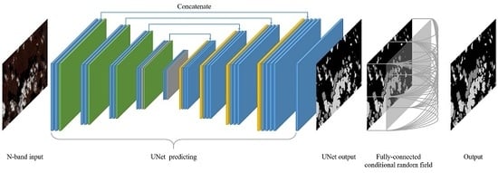
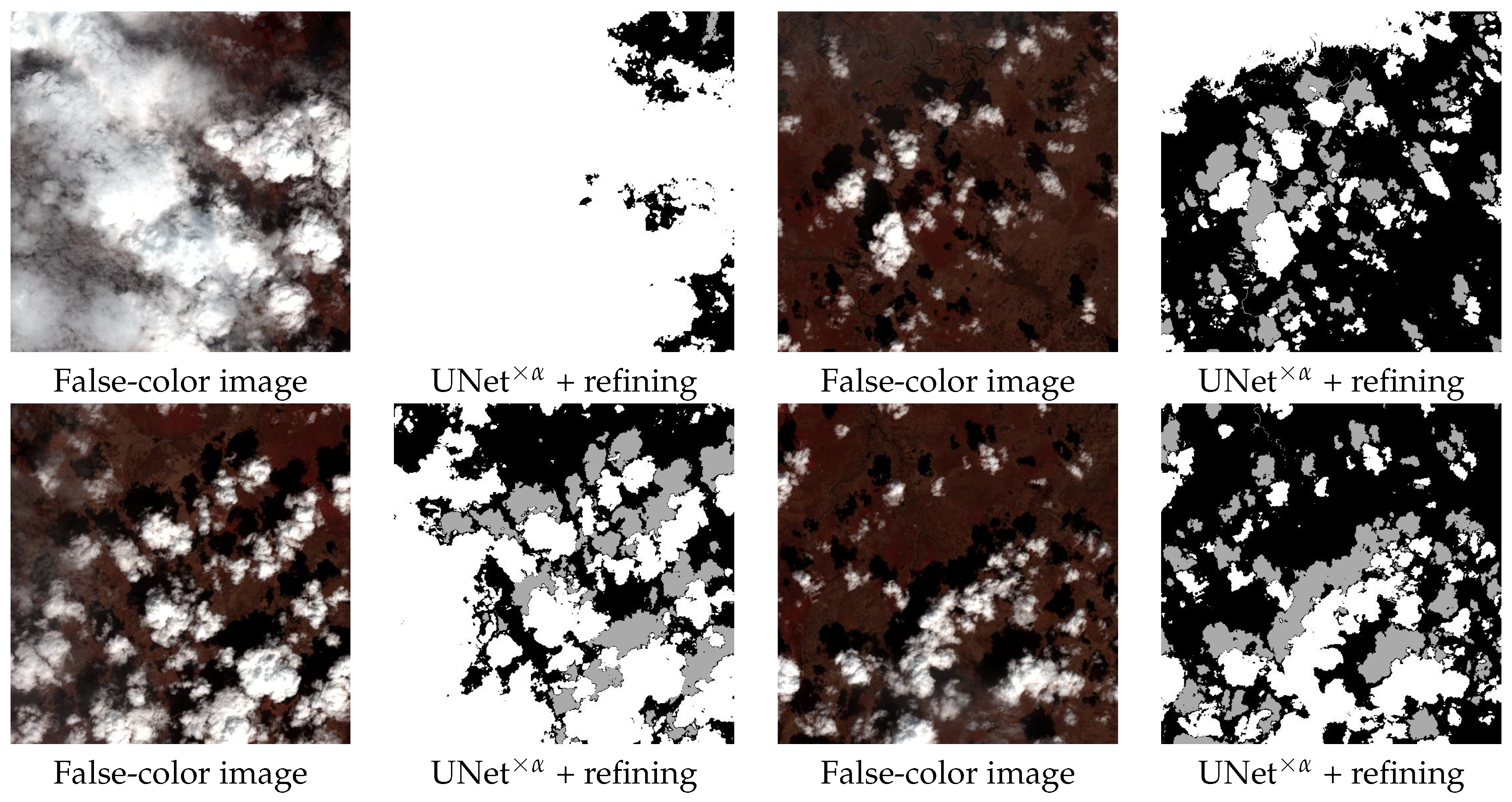
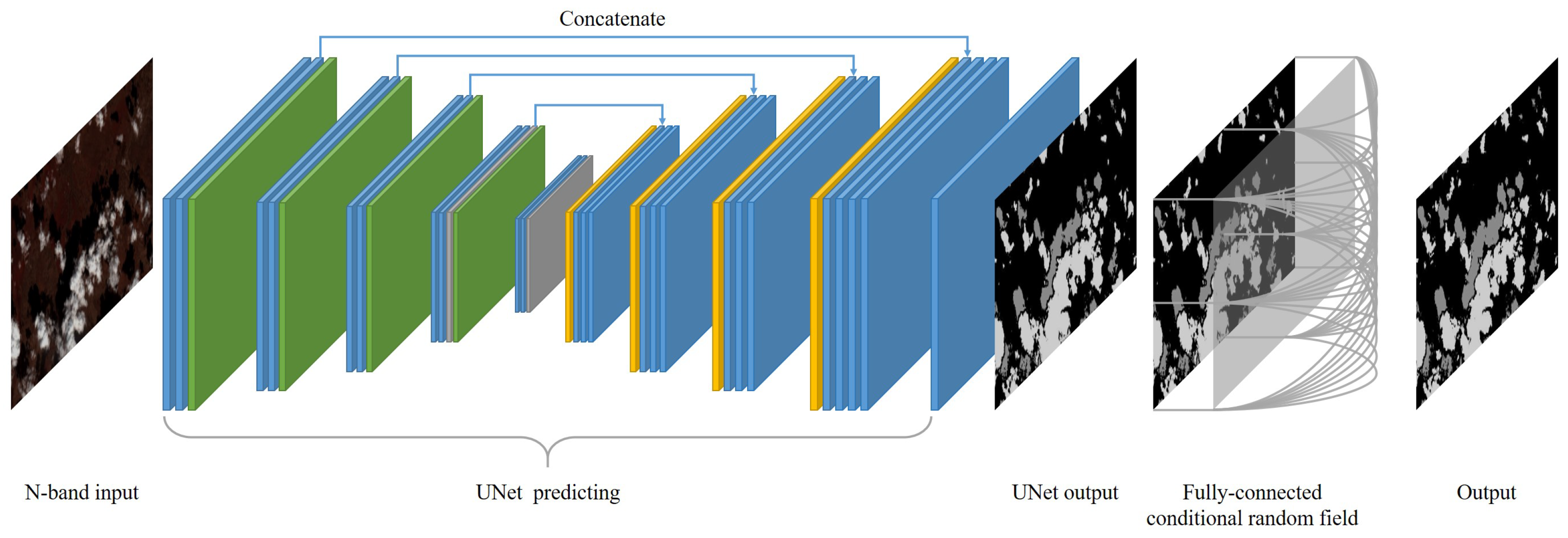
• Refined UNet: We propose an innovative architecture of assembling UNet and Dense CRF to detect clouds and shadows and refine their corresponding boundaries. The proper utilization of the Dense CRF refinement can sharpen the detection of cloud and shadow boundaries.
• Adaptive weights for imbalanced categories: An adaptive weight strategy for imbalanced categories is employed in training, which can dynamically calculate the weights and enhance the label attention of the model for minorities.
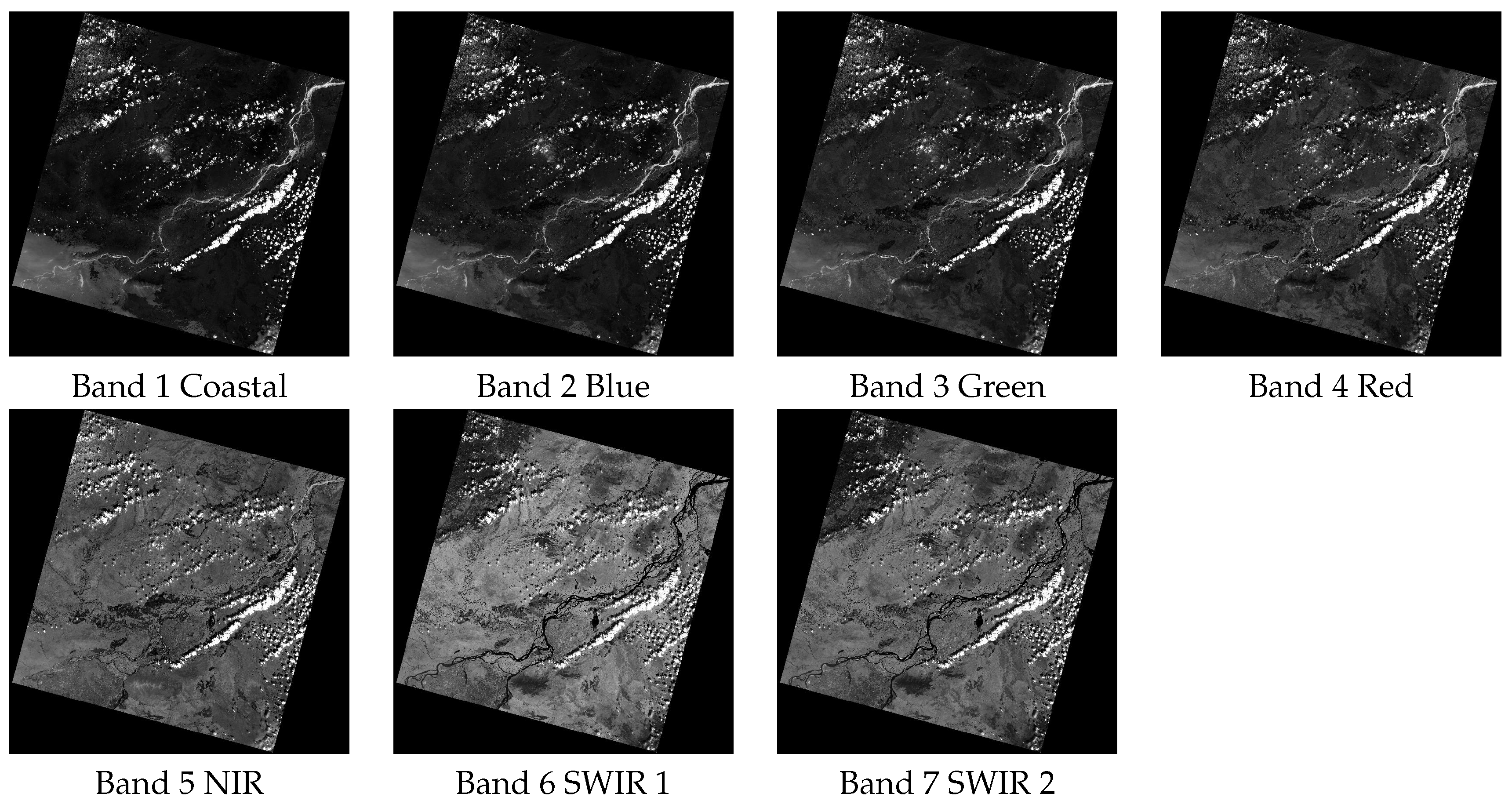
• Extension to four-band segmentation: The segmentation efficacy of our Refined UNet was also tested on the Landsat 8 OLI imagery dataset of Blue, Green, Red, and NIR bands; the experimental results illustrate that our method can obtain feasible segmentation results as well.

The rest of the paper is organized as follows. Section 2 investigates and presents some related work regarding cloud and cloud shadow detection and neural semantic segmentation. Proposed Refined UNet for cloud and shadow detection is described in Section 3. Section 4 presents the test Landsat8 OLI dataset, implementation details, and experiments for evaluation; it also illustrates experimental results qualitatively. Section 5 concludes this paper.

2. Related Work

We summarize the related work from two aspects: manual cloud and shadow segmentation in Section 2.1 and state-of-the-art neural semantic segmentation in Section 2.2.

2.1. Cloud and Shadow Segmentation

In terms of different perspectives of intermediate spectral features from remote sensing imageries, manually-developed cloud and corresponding shadow segmentation can be grouped into three categories: spectral tests, temporal differentiation, and statistical methods [1]. Observing the distribution of spectral data, thresholds were used to detect clouds and shadows limited in a finite range [9,10,11,12]. CFMask [13,14] explored comprehensively the spectral features and provided a benchmark of cloud and shadow detection. Temporal differentiation methods [15,16,17] observed the movement of dynamic clouds and shadows, detecting according to differences between imageries. Exploiting the statistics of spatial and spectral features, statistical methods [18,19] formulated detecting the cloud and shadow areas as a pixel-wise classification issue, which are highly relevant to data-driven methods. In this case, however, accurate or precise labels should be given so the statistical model can fit the distribution of cloud and shadows. Recently, it is noted that the cloud and shadow detection can be formulated as a semantic segmentation issue and solved by CNN-based pixel-wise classification model [1] when the data-driven methods thrived in semantic segmentation tasks on natural images; this is the main inspiration of formulating our task as well.

2.2. State-of-the-Art Neural Semantic Segmentation

Dense classification tasks, i.e., semantic segmentation tasks, aim to group pixels of an image into categories semantically, in which pixels of a potential object should be classified into a category. High-level vision tasks (image classification, object detection, etc) comprehend the high-level semantic information, whereas the low-level vision task provides a base for fine-grained image understanding. Accordingly, some representative and state-of-the-art methods are summarized as follows.

Classifiers of natural image segmentation tasks recognize natural objects and classify pixels accordingly: they take natural images as input and ultimately aim to output labeled predictions. These classifiers are seldom trained from scratch; they, alternatively, finetune feature extractors or other components of widely-used pretrained neural classifiers as the backbone networks. Typical backbones include VGG-16/VGG-19 [2], MobileNets V1/V2/V3 [20,21,22], ResNet18/ResNet50/ResNet101 [3,23], DenseNet [4], etc. The aforementioned backbone networks have demonstrated their striking performance in image classification tasks because of delicate feature extractor designing, which can effectively be transferred into the segmentation tasks as well.

Based on these backbone networks, neural semantic segmentation networks have significantly pushed the performance of pixel-level annotation tasks. Fully convolutional networks (FCN) [5] substituted fully-connected layers with convolutional layers, which can adaptively segment images with arbitrary sizes. U-Net [6] introduced intermediate feature fusion by concatenating multi-level feature maps with the same dimensions via shortcut connections, which popularized the reuse of features in image segmentation tasks. SegNet [7,8] inherited the encoder–decoder architecture and was applied to efficient scene understanding applications. Jegou et al. [24] extended DenseNet [4] into semantic segmentation problems due to its excellent performance on image classification tasks. FastFCN [25] used Joint Pyramid Upsampling to reduce computation complexity.

Explorations have been deep developed on feature mechanisms and data distributions: methods based on dilated convolution balanced trade-off between the larger receptive fields and kernel sizes, which implements multi-scale sparse subsampling with a small kernel and different dilated ratios. Yu et al. [26] proposed a method of multi-scale contextual aggregation using dilated convolutions. RefineNet [27] exploited fine-grained features to reinforce high-resolution classification in a way of building long-range residual connections (identity maps). PSPNet [28] aggregated global feature representations using Pyramid Pooling Module to segment images. Peng et al. [29] suggested that large kernel matters in the classification and localization tasks simultaneously, and accordingly proposed a global convolutional network to address mentioned issues. UPerNet [30] was proposed to discover rich visual knowledge and parse multiple visual concepts at once. HRNet [31] aggregated features from all the parallel convolutions instead of only from the high-resolution convolutions, leading to learning stronger feature representations. Gated-SCNN [32] built a two-stream segmentation classifier using a side branch of dedicated shape processing. Papandreou et al. [33] applied EM [34] to weakly- and semi-supervised learning for neural semantic segmentation.

DeepLabs initiated a series of segmentation methods along with the development of the mentioned methods. Using the atrous convolution and CRF, DeepLab V1 [35] initiated a pipeline aggregating rough classification and boundary refinement, and further DeepLab V2 [36] improved the performance. DeepLab V3 [37] deceased the use of CRF to improve segmentation performance. DeepLab V3+ [38] applied the depthwise separable convolution from Xception [39] to the atrous spatial pyramid pooling modules and decoder, promoting both efficiency and robustness.

Additionally, modeling segmentation as a probabilistic graphical model is gradually becoming a novel trend under the condition of CNN extracting high-level visual features. CRFasRNN [40] formulated CRF implementation as an RNN-based layer, which achieved an end-to-end training and inference of neural network predicting and CRF refining in natural image segmentation tasks. Deep parsing network [41] addressed the semantic segmentation task by modeling unary terms and pairwise terms from CNN and approximation of mean-field of additional layers, respectively, yielding a striking performance on PASCAL VOC 2012. Moreover, a combination of Gaussian Conditional Random Field (G-CRF) and deep learning architecture [42] is proposed to address the structured prediction, which inherited several merits including a unique global optimum, end-to-end training, and self-discovered pairwise terms.

Segmentation methods have carried out comprehensive exploration of semantic object localization, and have achieved promising performance on the dense classification tasks. The lower-level issues, however, should be concentrated carefully: splitting objects along with a precise boundary remains challenging, especially in remote sensing data. Consequently, we rethink the drawbacks of cloud and shadow detection and focus on the boundary prediction, which drives us to establish a dedicated model from scratch.

3. Methodology

In this section, we present the proposed Refined UNet in three subsections: The UNet architecture is introduced in Section 3.1 and the postprocessing of fully-connected conditional random field is presented in Section 3.2. The concatenation of UNet prediction and Dense CRF refinement is introduced in Section 3.3, which is also an overall framework. The entire pipeline of our method is illustrated in Figure 2.

3.1. UNet Prediction

UNet has been referred to as an effective structure in image segmentation tasks. Given an image of which each pixel is grouped into a specific category, UNet architecture can hierarchically extract low-level features and recombine them into higher-level features in the encoder, while it can perform the element-wise classification from multiple features in the decoder. Driven by the weighted cross-entropy loss function, UNet gradually secures the learnable parameters in feature extractors and infer the expected output which is closer to ground truth. The encoder–decode architecture of UNet is illustrated in Figure 3, in which down-sampling blocks of “Conv-ReLU-MaxPooling” are employed to extract features and upsampling blocks of “UpSample-Conv-ReLU” are employed to infer the segmentation in the same resolution.

To clarify the use of UNet architecture, a mathematical formulation of learning and inference is given as follows. In the learning phase, given the N-band input x that denotes a multi-band remote sensing image, UNet $f^{\mathrm{UNet}}$ outputs the logits $\widehat{y}$ with respect to x, in which $\widehat{y}$ denotes the corresponding pixel-wise likelihood.

$$\widehat{y}=f^{\mathrm{UNet}}\left(x\right)$$

(1)

Convolutional operator * filters the multi-band input or intermediate feature maps to generate multi-level features within $f^{\mathrm{UNet}}$ of N layers, in which each element ${\varphi }_{p,q,k}^l$ of the feature map of layer l are calculated in Equation (2).

$${\varphi }_{p,q,k}^l=\sum _c\sum _i\sum _j{\varphi }_{p+i,q+j,c}^{l-1}\times w_{i,j,c,k}+b_k$$

(2)

Following convolutional layers, MaxPooling layers are used to enlarge the receptive field so that high-level features can be captured comprehensively.

$f^{\mathrm{UNet}}(·)$ fuses the intermediate feature maps by concatenating them with the same size, in Equation (3).

$${\varphi }^l=[{\varphi }^{N-l+1},{\varphi }^{l-1}]$$

(3)

In our study, a weighted multi-class cross-entropy loss function with an adaptive categorical weight vector $\alpha$ is proposed to push the network to pay more attention to the minorities of categories. Specifically, ${\alpha }_i\in \alpha$ is proportion to the inverse of total counts $M_i$ of category i and the total counts of pixels M, namely, minorities in the categories can have higher weights. Thus, the loss function is calculated in Equation (4).

$${\mathcal{L}}^{\mathrm{seg}}(y,\widehat{y})=-{(\alpha \odot y)}^{\mathrm{T}}log\mathrm{softmax}\left(\widehat{y}\right)$$

(4)

in which $\mathrm{softmax}(·)$ denotes the softmax function defined by Equation (5).

$$\mathrm{softmax}\left(\widehat{y}\right)=\frac{exp\left(\widehat{y}\right)}{1^{\mathrm{T}}exp\left(\widehat{y}\right)}$$

(5)

where y denotes a one-hot vector of the label, $\widehat{y}$ is the prediction of $f^{\mathrm{UNet}}$ with respect to input x, and $\alpha$ is the adaptive weight vector of each category. Each element of $\alpha$ is calculated dynamically in Equation (6).

$${\alpha }_i=\frac{1}{M_i}max\left(M\right)$$

(6)

where ${\alpha }_i$ denotes the adaptive weight of category i and $M_i$ is the total counts of category i.

In the optimization, the gradient descent method is used to optimize the learnable parameters in UNet, more specifically, kernels of convolutional layers. Particularly, the derivatives of the loss function with respect to the output $\widehat{y}$ is calculated in Equation (7).

$$\frac{\partial {\mathcal{L}}_{\mathrm{seg}}}{\partial \widehat{y}}=\mathrm{softmax}\left(\widehat{y}\right)-(\alpha \odot y)$$

(7)

In the inference phase, UNet outputs the segmentation proposal with the size of $p\times q\times k$ indicating that $p\times q$ pixels have the possibilities of k categories. The maximums of these k possibilities are the elementwise classification results.

$$c_{p,q}=arg\underset{k}{max}{\widehat{y}}_{p,q,k}$$

(8)

3.2. Fully-Connected Conditional Random Field (Dense CRF) Postprocessing

Generally speaking, UNet can reliably sense the existence of clouds and cloud shadows and roughly localize them. The boundaries of clouds, however, cannot be precisely pinpointed by UNet. The reason for vague boundary segmentation is speculated as follows: multiple max-pooling layers enlarge the receptive field of the neural network, which improves effectively extracting the high-level features (i.e., semantic information) and helps high-level vision tasks, for instance, image classification. However, the use of multiple max-pooling layers brings more invariance in the low-level vision tasks, which is detrimental to exact boundary detection in cloud segmentation [35]. UNet is still affected in fine-grained segmentation even if the concatenations attempt to alleviate the lack of high-resolution features. Considering the disadvantages of UNet prediction, the postprocessing of the fully-connected conditional random field (Dense CRF) is employed to refine exact cloud boundaries.

The cloud and shadow refinement of Dense CRF is formulated as follows. Element-wise classification $(\mathsf{X},\mathsf{I})$ can be formulated as a conditional random field (CRF) characterized by a Gibbs distribution, defined in Equation (9).

$$P(\mathsf{X}=\mathsf{x}|\mathsf{I})=\frac{1}{Z\left(\mathrm{I}\right)}exp(-E\left(\mathsf{x}\right|\mathsf{I}))$$

(9)

in which $E\left(x\right)$ denotes the Gibbs energy, $\mathcal{G}=(\mathcal{V},\mathcal{E})$ the graph, $\mathcal{V}=\{X_1,X_2,\cdots ,X_N\}$ the element-wise classes, $\mathsf{I}$ the global observation (image), and $Z\left(\mathsf{I}\right)$ the normalization term to guarantee the correct probability.

In the Dense CRF, the corresponding Gibbs energy function is defined in Equation (10).

$$E\left(\mathsf{x}\right)=\sum _i{\psi }_u\left(x_i\right)+\sum _i\sum _{i<j}{\psi }_p(x_i,x_j)$$

(10)

in which $\mathsf{x}$ denotes the label assignment for all pixels, ${\psi }_u$ the unary potential, and ${\psi }_p$ the pairwise potential.

The unary potential ${\psi }_u\left(x_i\right)$ can be given by UNet outputs, while the pairwise potential ${\psi }_p\left(x_i\right)$ is defined in Equation (11).

$${\psi }_p(x_i,x_j)=\mu (x_i,x_j)\underset{k({\mathsf{f}}_i,{\mathsf{f}}_j)}{\underbrace{\sum _{m=1}^K{w}^{\left(m\right)}{k}^{\left(m\right)}({\mathsf{f}}_i,{\mathsf{f}}_j)}}$$

(11)

in which $\mu (x_i,x_j)$ denotes the label compatibility in Dense CRF and ${\mathsf{f}}_i$ and ${\mathsf{f}}_j$ the feature vectors. In our case, Potts model $\mu (x_i,x_j)=[x_i\ne x_j]$ is used as the label compatibility.

Contrast-sensitive two-kernel potentials [43] are used to capture the connectivity of two nearby pixels with similar spectral features and eliminate the isolated regions, defined in Equation (12).

$$\begin{array}{cc}\hfill k({\mathsf{f}}_i,{\mathsf{f}}_j)=& w^{\left(1\right)}exp\left(-\frac{|p_i-p_j{|}^2}{2{\theta }_{\alpha }^2}-\frac{|I_i-I_j{|}^2}{2{\theta }_{\beta }^2}\right)\hfill \\ \hfill & +w^{\left(2\right)}exp\left(-\frac{|p_i-p_j{|}^2}{2{\theta }_{\gamma }^2}\right)\hfill \end{array}$$

(12)

in which $p_i$, $p_j$ denote the positions, $I_i$, $I_j$ the spectral features of pixel i and j. The spectral features $I_i$ and $I_j$ consist of false-color band 5, 4, and 3. Note that ${\theta }_{\alpha }$, ${\theta }_{\beta }$, and ${\theta }_{\gamma }$ are three key hyperparameters controlling the degree of connectivity and similarity, and significantly affect the performance of the refinement.

In the inference phase, the Dense CRF infers an observation $\widehat{\mathsf{x}}$ to find the most likely assignment (MAP) of $P\left(\mathsf{x}\right)$: $\widehat{\mathsf{x}}=arg{max}_{\mathsf{x}}P\left(\mathsf{x}\right)$ where $P\left(\mathsf{x}\right)=1/Zexp(-E(\mathsf{x}\left)\right)$. An efficient solution to Dense CRF has been provided in [43], in which the approximate inference of the iterative message-passing algorithm is used to estimate the CRF distribution. The solution facilitates the inference of Dense CRF in a linear time complexity, which can result in an efficient utility of Dense CRF in segmentation tasks.

3.3. Concatenation of UNet Prediction and Dense CRF Refinement

The overall framework of our Refined UNet is described as follows. The large size of an entire high-resolution remote sensing image discourages UNet prediction; predicting patch by patch, therefore, is a practical solution to the remote sensing image. Cropped into and reconstructed from tiles, the multi-band remote sensing image is transformed into a segmentation proposal by UNet. Afterward, Dense CRF can sufficiently process the entire image, which can improve the prediction coherency on the edges of tiles and eliminate isolated regions. Specifically, the concatenation of UNet prediction and Dense CRF refinement is described as follows:

• The entire images are rescaled, padded, and cropped into patches with the size of $w^{\mathrm{crop}}\times h^{\mathrm{crop}}$. The trained UNet infers the pixel-level categories for the patches. The rough segmentation proposal is constructed from the results.
• Taking as input the entire UNet proposal and a three-channel edge-sensitive image, Dense CRF refines the segmentation proposal to make the boundaries of clouds and shadows more precise.

We observed in the experiments the efficacy of patch-wise UNet prediction and Dense CRF refinement.

4. Experiments and Discussion

Experiments were conducted to evaluate the results of our Refined UNet compared to references. Ablation studies are conducted to verify the efficacy of each component as well. Experimental data acquisition, implementation details, and evaluation metrics are briefly introduced in Section 4.1, Section 4.2, and Section 4.3, respectively. In Section 4.4, Refined UNet and novel methods are compared and evaluated qualitatively and quantitatively. In Section 4.5, the outputs of Refined UNet and references are visually compared, in which the superiority of boundary refinement can be illustrated. In Section 4.6, the refinement of Dense CRF is evaluated in against with vanilla UNet predictions. In Section 4.7, some key hyperparameters are examined to show the effect on the segmentation performance. In Section 4.8, the effect of adaptive weights for imbalanced categories is evaluated against fixed weights. In Section 4.9, cross-validation on the four-year dataset is used to explore the performance consistency. At last, evaluations on four-band imageries and comparisons are conducted in Section 4.10.

4.1. Experimental Data Acquisition and Preprocessing

In the experiments, Landsat 8 OLI imagery data [11] were employed to train, validate, and test the performance of our Refined UNet. We chose images in the years of 2013, 2014, and 2015 and split them into the training set and validation set. Images in 2016 were chosen as the test data for visualization and numerical evaluation. Cloud and shadow labels were generated from the Pixel Quality Assessment band, in which the clouds and shadows with confidence were derived from the CFMask algorithm. Practically, clouds and shadows with high confidence were marked while those with low confidence were excluded. Class IDs of background, fill values, shadows, and clouds are 0, 1, 2, and 3, respectively; alternatively, we merged classes of land, snow, and water into that of background because segmentation tasks of clouds and cloud shadows are the key issue we are discussing. Instead of ground truths, the labels are referred to as references because they are dilated and not accurate enough at the pixel level. All seven bands were merged as default inputs, as illustrated in Figure 4. For visual evaluation, Band 5 NIR, 4 Red, and 3 Green were combined as RGB channels to construct a false-color image. Linear 2% algorithm was performed on the false-color images to enhance the contrast and visualization. The false-color images were still used as the inputs of Dense CRF because of its sufficient contrast and evident edges. Additionally, Bands 2 Blue, 3 Green, 4 Red, and 5 NIR in Landsat 8 OLI data were chosen to combine the inputs of four-band images. We assessed the segmentation performance compared to seven-band segmentation.

The training, validation, and test sets are listed as follows. Training set:

• 2013: 2013-04-20, 2013-06-07, 2013-07-09, 2013-08-26, 2013-09-11, 2013-10-13, and 2013-12-16
• 2014: 2014-03-22, 2014-04-23, 2014-05-09, 2016-06-10, and 2014-07-28
• 2015: 2015-06-13, 2015-07-15, 2015-08-16, 2015-09-01, and 2015-11-04

Validation set:

• 2013: 2013-06-23, 2013-09-27, and 2013-10-29
• 2014: 2014-02-18, and 2014-05-25
• 2015: 2015-07-31, 2015-09-17, and 2015-11-20

Test set:

• 2016: 2016-03-27, 2016-04-12, 2016-04-28, 2016-05-14, 2016-05-30, 2016-06-15, 2016-07-17, 2016-08-02, 2016-08-18, 2016-10-21, and 2016-11-06

In the preprocessing, images were padded firstly for slicing. Zeros were assigned to fill values and surrounding padded values. The padded size was calculated using Equations (13)–(16), respectively, where $w^{\mathrm{l}}$, $w^{\mathrm{r}}$, $h^{\mathrm{u}}$, and $h^{\mathrm{d}}$ denote the left, right, up, and down padding widths and heights. After padding, we cropped raw image data into $512\times 512$ patches for training, validation, or test.

$$\begin{array}{cc}\hfill w^{\mathrm{l}}& =\lfloor \frac{1}{2}(w^{\mathrm{crop}}-(w^{\mathrm{raw}}mod{w}^{\mathrm{crop}}))\rfloor \hfill \end{array}$$

(13)

$$\begin{array}{cc}\hfill w^{\mathrm{r}}& =w^{\mathrm{crop}}-w^{\mathrm{l}}\hfill \end{array}$$

(14)

$$\begin{array}{cc}\hfill h^{\mathrm{u}}& =\lfloor \frac{1}{2}(h^{\mathrm{crop}}-(h^{\mathrm{raw}}mod{h}^{\mathrm{crop}}))\rfloor \hfill \end{array}$$

(15)

$$\begin{array}{cc}\hfill h^{\mathrm{d}}& =h^{\mathrm{crop}}-h^{\mathrm{u}}\hfill \end{array}$$

(16)

Data normalization used Equation (17) to rescale features into interval $[0,1]$.

$$x_{ijk}^{*}=\frac{x_{ijk}-min\left(x\right)}{max\left(x\right)-min\left(x\right)+ϵ}$$

(17)

in which $ϵ$ is ${10}^{-10}$ to avoid that data are divided by zero.

4.2. Implementation Details

The UNet model is composed of four “Conv-BN-ReLU” components for down-sampling and four “UpSample-Conv-BN-ReLU” components for up-sampling. The model was trained from scratch on the training set, taking as input seven- or four-band imageries and outputting 0– to label each pixel. It was optimized by ADAM [44] optimizer in which ${\beta }_1$, ${\beta }_2$, and learning rate were 0.9, 0.999, and 0.001, respectively.

As the postprocessing, Dense CRF took as input both the entire false-color images and categorical proposals reconstructed from UNet results and transforms into refined predictions. Empirically, the default ${\theta }_{\alpha }$, ${\theta }_{\beta }$, and ${\theta }_{\gamma }$ were 80, 13, and 3. We further conducted subsequent experiments to thoroughly test the effect of Dense CRF with regards to the aforementioned hyperparameters.

4.3. Evaluation Metrics

In our four-class pixel-level classification task, precision P, recall R, and F1 score $F_1$ were utilized to evaluate the efficacy and sensitivity of the cloud and shadow detection. Considering the confusion matrix $P^{\mathrm{cm}}={\left[p_{ij}\right]}_{4\times 4},i,j\in \{0,1,2,3\}$, in which $p_{ij}$ denotes the number of observations that should actually belong to group i and are predicted to group j, precision reports how many correct pixels in the prediction the method can retrieve, defined in Equation (18); recall reports how comprehensively the method can retrieve specified pixels, defined in Equation (19); and F1 score is a numerical assessment taking into consideration both precision and recall, defined in Equation (20).

$$P_i=\frac{p_{ii}}{{\sum }_{i=1}^C{p}_{ij}}$$

(18)

$$R_i=\frac{p_{ii}}{{\sum }_{j=1}^C{p}_{ij}}$$

(19)

$$F_{1i}=2\times \frac{P_i·R_i}{P_i+R_i}$$

(20)

In addition, Wilcoxon signed-rank test [45] was used to test if the differences between the two methods are significant.

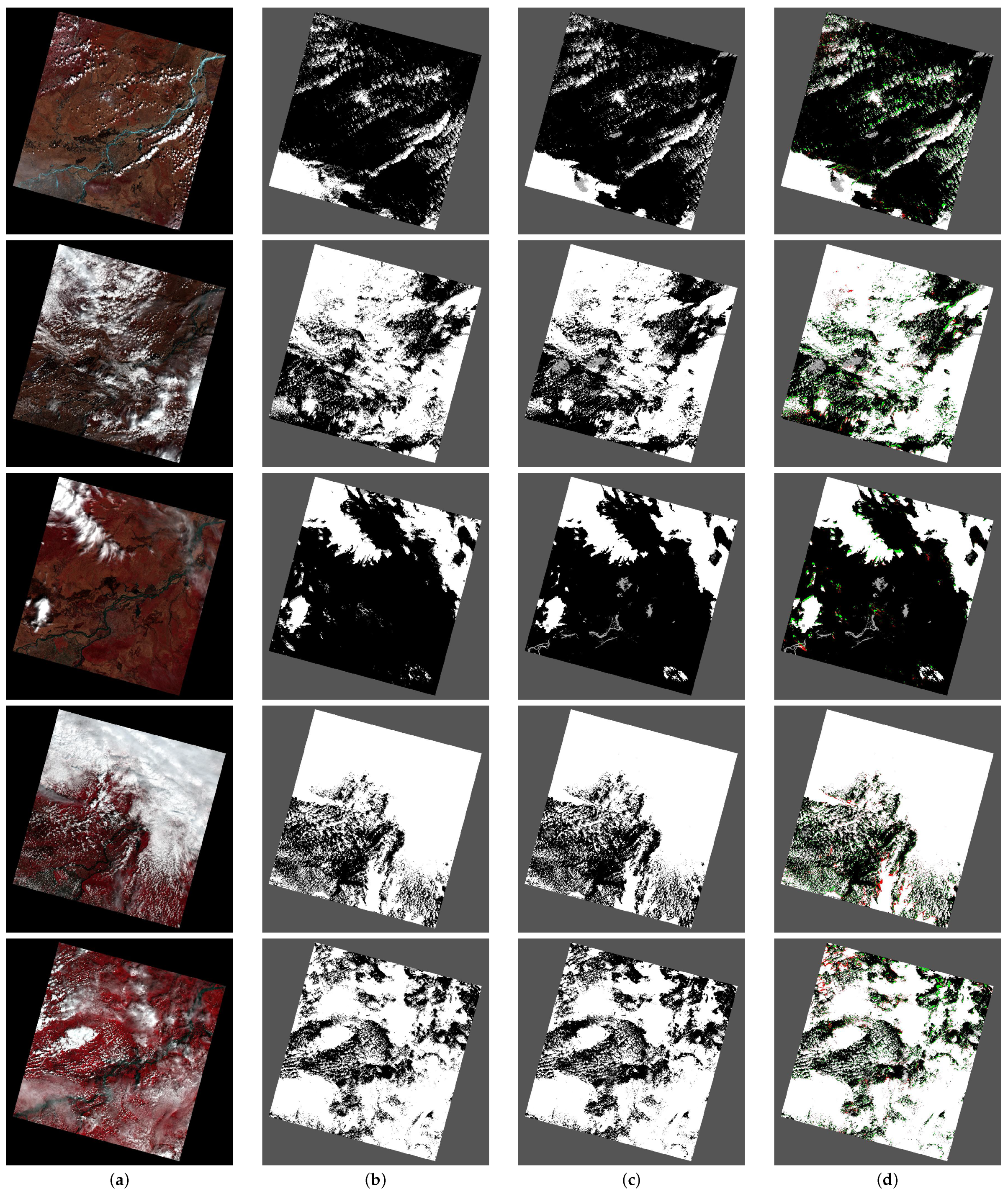
4.4. Comparisons of Refined UNet and Novel Methods

We first compared our Refined UNet to its backbone net UNet [6], which is usually exploited in natural image segmentation. Besides, the novel PSPNet [28] with ResNet-50 as the backbone net was retrained from scratch on the training set and its results are also taken into consideration. The same strategy of adaptive weights for imbalanced categories was used in the training of these methods. Qualitative and quantitative results are presented in Figure 5 and

Table 1. Average scores of accuracy, precision, recall, and F1 of PSPNet, the backbone (UNet), and Refined UNet. The top results are highlighted in bold.

Class No.	Class Name	Evaluation	PSPNet (%)	UNet (%)	Refined UNet (%)
		Accuracy+	84.88 ± 7.59	93.04 ± 5.45	93.51 ± 5.45
0	Background	Precision+	65.49 ± 19.62	93.34 ± 4.88	90.33 ± 7.04
		Recall+	98.57 ± 2.18	81.52 ± 15.3	85.58 ± 17.4
		F1+	77.06 ± 15.04	86.35 ± 11.04	86.92 ± 12.18
1	Fill Values	Precision+	100 ± 0	100 ± 0	99.89 ± 0.06
		Recall+	95.97 ± 0.19	100 ± 0	100 ± 0
		F1+	97.94 ± 0.1	100 ± 0	99.94 ± 0.03
2	Shadows	Precision+	46.81 ± 24.98	34.74 ± 14.77	36.28 ± 20.4
		Recall+	7.83 ± 5.95	54.31 ± 18.72	21.51 ± 11.91
		F1+	12.74 ± 9.14	40.43 ± 14.74	24.63 ± 11.49
3	Clouds	Precision+	94.09 ± 17	87.28 ± 18.78	87.57 ± 19.11
		Recall+	48.22 ± 22.81	95.96 ± 3.63	96.03 ± 3.17
		F1+	60.99 ± 22.56	90.12 ± 13.77	90.22 ± 14.09

.

Figure 5 shows the visualization results of PSPNet, UNet, and Refined UNet. It can be seen that our Refined UNet outperforms PSPNet in terms of visual detection of clouds and shadows: some clouds and shadows are missing in the detection of PSPNet, whereas UNet over-detects clouds and shadows. Refined UNet overcomes the drawbacks of over-detection and delineates the boundaries of clouds and shadows more precisely, compared to UNet. The cutting edges of tiles, on the other hand, are also neutralized in the results of Refined UNet, while those gaps of PSPNet are not properly sealed. In summary, our Refined UNet can effectively label rough clouds and shadows and refine their boundaries more precisely.

Table 1 shows the quantitative assessments with respect to PSPNet, UNet, and Refined UNet. Precision $P_i$ assesses the efficacy of how many pixels the method can correctly detect in its prediction of class i, while recall $R_i$ indicates the efficacy of how many pixels the method can sensitively capture in all pixels of a specified class i. F1 score $F_{1i}$ takes into consideration both the specificity and the sensitivity by computing the average of $P_i$ and $R_i$. In the detection of clouds and shadows, Refined UNet balances the performance of precisions and recalls, while PSPNet only achieves superior precisions due to its negligence of clouds and shadows with low confidence. It is concluded that Refined UNet can achieve superiority of balancing precision and recall in the precise detection of clouds and shadows.

4.5. Comparisons of References and Refined UNet

Next, we report the segmentation results and compare our results to the references from qualitative and quantitative perspectives. Figure 6 entirely illustrates the false-color visualizations, the segmentation references the results of Refined UNet, and the differences between them. We can generally conclude that our method can detect clouds comprehensively and precisely: in the visual assessment, almost all pixels of clouds can be detected correctly. The clouds and shadows can be considerably retrieved by the Refined UNet, especially for the interior pixels indicating clouds and shadows. Sharper boundaries of clouds and shadows are delineated and the pixels indicating differences are highlighted on the boundaries of clouds and shadows, which can illustrate the effect of Dense CRF refinement. In terms of the superior results, one of the merits of the Refined UNet, thus, is concluded: Refined UNet can almost detect all clouds and shadows with high confidence, and refine the boundaries of clouds, highlighted in difference visualization. We attribute this superiority to the nature that the UNet model can roughly locate clouds and shadows and Dense CRF can detect the explicit boundaries, which generates accurate and refined results.

Nevertheless, the drawback of refinement cannot be totally ignored: Refined UNet might over-refine the boundaries of shadows, which leads to missing the detection of some shadows. The difference images illustrated that in some cases, Dense CRF is strong in refinement so it inevitably erases some weak shadows, which shows its aggression. In fact, it appears to be a trade-off between specificity and sensitivity of the model, and, in our cases, the precision should be the first priority.

We further evaluated locally, by zooming into some areas and observing the rough location and refinement of the detection. Figure 7 visually confirms the superiority of refining the boundaries of clouds and shadows. Combining entirely and locally visual assessment, we conclude that our Refined UNet can accurately locate clouds and shadows and precisely capture boundaries.

We also evaluated our method from the quantitative perspective, in which precision, recall, and F1 score were employed to assess the performance of detection. Precision $P_i$ assesses the efficacy of how many pixels the method can correctly detect in its prediction of class i, while recall $R_i$ indicates the efficacy of how many pixels the method can sensitively capture in all pixels of a specified class i. F1 score $F_{1i}$ takes into consideration both the specificity and the sensitivity by computing the average of $P_i$ and $R_i$. Before evaluating, we hypothesize that precisions should be higher while recalls should be lower because of the fact of these indicators.

Table 2. Average scores of accuracy, precision, recall, and F1 for multiple UNet models with Dense CRF refinement. The top results are highlighted in bold.

Class No.	Class Name	Evaluation	UNet (%)	UNet${}^{\times 5}$ (%)	UNet${}^{\times 10}$ (%)	UNet${}^{\times 15}$ (%)	UNet${}^{\times 20}$ (%)	UNet${}^{\times \mathit{\alpha }}$ (%)
		Accuracy+	92.92 ± 6.68	92.89 ± 6.6	92.15 ± 6.89	91.81 ± 6.51	90.85 ± 6.85	93.51 ± 5.45
0	Background	Precision+	90.58 ± 7.73	91.75 ± 6.94	94.64 ± 4.72	95.23 ± 4.47	95.80 ± 3.98	90.33 ± 7.04
		Recall+	81.60 ± 26.76	80.11 ± 27.31	76.06 ± 28.00	75.01 ± 23.87	70.46 ± 27.14	85.58 ± 17.40
		F1+	83.15 ± 24.10	82.42 ± 25.37	80.24 ± 27.68	81.25 ± 20.76	77.20 ± 27.35	86.92 ± 12.18
1	Fill Values	Precision+	99.91 ± 0.05	99.89 ± 0.06	99.89 ± 0.06	99.88 ± 0.06	99.90 ± 0.04	99.89 ± 0.06
		Recall+	99.99 ± 0.00	99.99 ± 0.00	99.99 ± 0.00	99.99 ± 0.00	99.99 ± 0.00	99.99 ± 0.00
		F1+	99.95 ± 0.03	99.94 ± 0.03	99.94 ± 0.03	99.94 ± 0.03	99.95 ± 0.02	99.94 ± 0.03
2	Shadows	Precision+	48.69 ± 40.98	44.20 ± 23.46	36.64 ± 20.75	27.62 ± 13.33	23.39 ± 10.36	36.28 ± 20.40
		Recall+	1.01 ± 1.54	13.44 ± 11.37	21.55 ± 15.82	27.38 ± 16.51	35.92 ± 17.02	21.51 ± 11.91
		F1+	1.91 ± 2.86	18.78 ± 13.51	25.16 ± 16.28	26.25 ± 13.47	27.67 ± 12.23	24.63 ± 11.49
3	Clouds	Precision+	82.02 ± 19.64	81.99 ± 19.45	79.68 ± 19.94	80.52 ± 19.74	80.78 ± 19.82	87.57 ± 19.11
		Recall+	98.95 ± 0.81	99.03 ± 0.73	99.25 ± 0.63	99.20 ± 0.69	99.13 ± 0.71	96.03 ± 3.17
		F1+	88.19 ± 15.24	88.26 ± 14.97	86.84 ± 15.51	87.38 ± 15.37	87.50 ± 15.32	90.22 ± 14.09

confirmed our hypothesis.

In Table 2, the average precisions of backgrounds, fill values, and shadows are higher while clouds are slightly lower. We attribute the higher precisions to the Dense CRF refinement: it dramatically purifies the detection of shadows. The lower precision of clouds with high standard deviations may be caused by the misclassification of snow pixels, which strongly affects the performance of cloud detection. We will further investigate the differentiation of cloud and snow pixels to promote precisions.

4.6. Effect of the Dense CRF Refinement

An ablation study on the Dense CRF was conducted to test its effect. Dense CRF focuses on splitting along boundaries so that it can further obtain a finer segmentation result in the task. In addition to refining the contours precisely, Dense CRF can be used to eliminate isolated predictions (misclassification noises) and smooth gaps of slices practically. Figure 8 and Figure 9 qualitatively show the results with and without Dense CRF refinement. As shown in the figures, the boundaries of clouds and shadows are refined, and the isolated misclassification regions and slicing gaps are removed as well, which demonstrates the superiority of our Refined UNet. We also realize that the strong Dense CRF might also erase some small shadow patches with vague boundaries or some plausible shadow patches, which should be solved in the future.

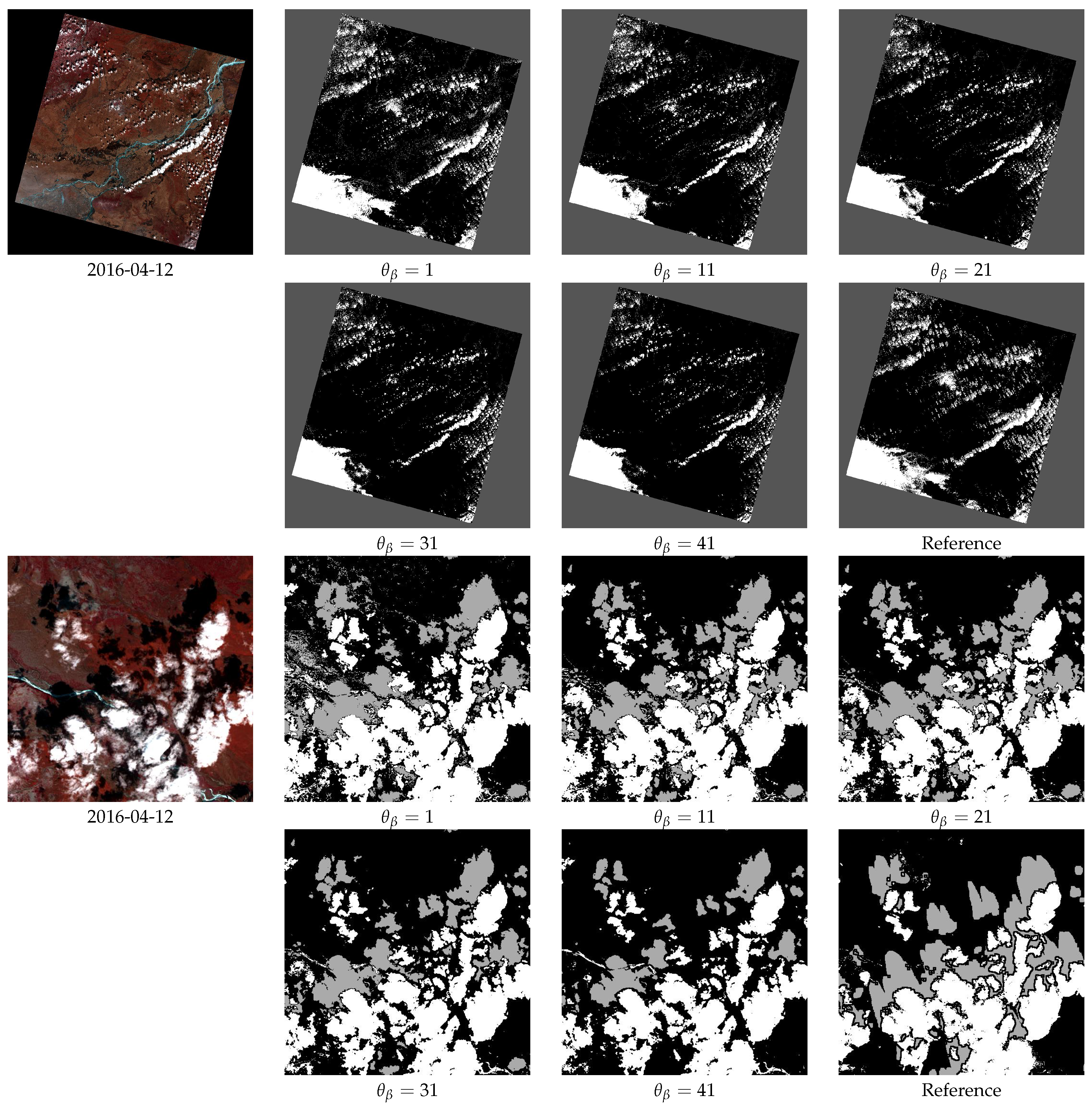
4.7. Hyperparameter Sensitivity with Respect to Dense CRF

We examined the performance of Dense CRF postprocessing by varying the spatial and spectral ranges in the appearance and smooth kernels ${\theta }_{\alpha }$, ${\theta }_{\beta }$, and ${\theta }_{\gamma }$, which is shown in Figure 10, Figure 11 and Figure 12. According to Krahenbuhl and Koltun [43], a proper ${\theta }_{\gamma }$ yields a slight visual improvement, which is visually demonstrated by Figure 12. Higher ${\theta }_{\alpha }$ and ${\theta }_{\beta }$, on the other hand, provide more visual improvement and remove more isolated regions. However, they can over-refine the cloud and shadow regions as well. In summary, these parameters should be learned using more accurately labeled data or controlled manually.

4.8. Effect of the Adaptive Weights Regarding Imbalanced Categories

The adaptive weights with regard to imbalanced categories were employed to promote the performance of cloud and shadow detection. By observing imagery data of the whole year, the clouds and shadows may be minorities in summer and autumn, which needs to dynamically balance the training samples. Hence, the adaptive weights are required to balance. Figure 13 and Figure 14 show the comparisons between segmentation results with the fixed weights and the adaptive weight. Fixed weights drive UNet to predict more shadows even though it seems that the model would over-detect: it captures more pixels that should not be grouped into the category of shadows. Note that more cloud shadows of isolated pixels are also detected in our case. Adaptive weights adjust the prediction dynamically, fit the distribution of cloud and shadow pixels, and push the model to classify properly. We conclude that our method can achieve a good performance in finely detecting clouds and shadows, in terms of visual assessments.

Quantitative assessments were used to demonstrate the superiority of our method. F1 score was used to numerically demonstrate it since it considers both precision and recall. In Table 2 and

Table 3. Average scores of accuracy, precision, recall, and F1 for multiple UNet models without Dense CRF refinement. The top results are highlighted in bold.

Class No.	Class Name	Evaluation	UNet (%)	UNet${}^{\times 5}$ (%)	UNet${}^{\times 10}$ (%)	UNet${}^{\times 15}$ (%)	UNet${}^{\times 20}$ (%)	UNet${}^{\times \mathit{\alpha }}$ (%)
		Accuracy+	93.1 ± 6.45	93.02 ± 6.29	91.91 ± 6.81	91.59 ± 6.41	90.47 ± 6.84	93.04 ± 5.45
0	Background	Precision+	92.84 ± 5.81	94.50 ± 5.13	96.72 ± 2.98	97.87 ± 1.72	97.94 ± 1.73	93.34 ± 4.88
		Recall+	81.83 ± 24.23	78.88 ± 24.23	73.91 ± 25.79	73.23 ± 20.10	67.95 ± 25.57	81.52 ± 15.30
		F1+	84.91 ± 20.54	83.83 ± 21.25	80.78 ± 24.42	82.15 ± 16.06	76.87 ± 25.55	86.35 ± 11.04
1	Fill Values	Precision+	99.99 ± 0.00	99.98 ± 0.01	99.99 ± 0.01	99.99 ± 0.00	99.99 ± 0.00	99.99 ± 0.00
		Recall+	99.99 ± 0.00	99.99 ± 0.00	99.99 ± 0.00	99.99 ± 0.00	99.99 ± 0.00	99.99 ± 0.00
		F1+	99.99 ± 0.00	99.99 ± 0.01	99.99 ± 0.01	99.99 ± 0.00	99.99 ± 0.00	99.99 ± 0.00
2	Shadows	Precision+	63.65 ± 38.27	46.68 ± 20.38	34.72 ± 15.54	28.56 ± 12.45	25.40 ± 11.44	34.74 ± 14.77
		Recall+	5.35 ± 6.17	30.36 ± 20.30	39.33 ± 22.31	49.08 ± 19.79	57.49 ± 21.22	54.31 ± 18.72
		F1+	9.38 ± 10.27	34.15 ± 18.25	35.66 ± 16.76	35.45 ± 14.54	34.67 ± 14.56	40.43 ± 14.74
3	Clouds	Precision+	80.39 ± 19.34	80.80 ± 19.24	78.98 ± 19.79	80.62 ± 19.47	80.65 ± 19.82	87.28 ± 18.78
		Recall+	99.43 ± 0.87	99.49 ± 0.62	99.59 ± 0.59	99.42 ± 0.67	99.21 ± 0.79	95.96 ± 3.63
		F1+	87.45 ± 15.10	87.77 ± 14.82	86.57 ± 15.41	87.59 ± 15.07	87.49 ± 15.15	90.12 ± 13.77

, we find that the UNet with adaptive weights significantly outperforms the models with fixed weights in terms of F1 scores, which also supports the conclusion of qualitative assessments.

4.9. Cross-Validation over the Entire Dataset

We further evaluated the performance consistency of our Refined UNet by the cross-validation upon the image set of each year. For all images used above, five images for each year were selected and are listed as follows. For the four cross-validations, images of two years were used as the training set, one year as the validation set, and the last one as the test set. The quantitative results are reported in

Table 4. Average scores of accuracy, precision, recall, and F1 of Refined UNet on cross-validation of the four-year image set.

Class No.	Class Name	Evaluation	2013 (%)	2014 (%)	2015 (%)	2016 (%)
		Accuracy+	88.35 ± 9.4	93.23 ± 8.87	92.36 ± 4.14	89.1 ± 3.48
0	Background	Precision+	89.22 ± 7.35	95.98 ± 2.43	95.33 ± 3.29	93.56 ± 4.16
		Recall+	79.29 ± 28.77	84.73 ± 26.05	85.91 ± 12.32	65.24 ± 28.75
		F1+	82 ± 22.23	87.93 ± 18.74	89.98 ± 7.53	73.12 ± 25.75
1	Fill Values	Precision+	99.98 ± 0.01	99.96 ± 0.03	99.95 ± 0.04	99.96 ± 0.03
		Recall+	100 ± 0	100 ± 0	100 ± 0	100 ± 0
		F1+	99.99 ± 0.01	99.98 ± 0.02	99.98 ± 0.02	99.98 ± 0.01
2	Shadows	Precision+	7.25 ± 5.3	6.96 ± 9.76	26.65 ± 17.78	15.26 ± 6.28
		Recall+	18.95 ± 17.61	5.16 ± 6.17	45.99 ± 14.27	54.4 ± 12
		F1+	6.33 ± 3.2	5.59 ± 7.76	31.38 ± 14.82	23.65 ± 9.06
3	Clouds	Precision+	90.63 ± 19.24	85.74 ± 17.37	92.57 ± 6.32	93.52 ± 8.05
		Recall+	76.06 ± 36.04	89.51 ± 14.2	92.31 ± 9.67	84.35 ± 17.64
		F1+	75.57 ± 31.36	85.77 ± 11.19	91.97 ± 4.23	87.59 ± 11.21

. The accuracy, precision, recall, and f1 score can demonstrate the performance consistency of our Refined UNet: all of them can perform well on labeling pixels of background, fill values, and clouds, in terms of precisions. Labeling the pixels of shadows, however, should be improved as plenty of detection algorithms do.

• 2013: 2013-04-20, 2013-06-07, 2013-07-09, 2013-08-26, and 2013-09-11
• 2014: 2014-03-22, 2014-04-23, 2014-05-09, 2014-06-10, and 2014-07-28
• 2015: 2015-06-13, 2015-07-15, 2015-08-16, 2015-09-01, and 2015-11-04
• 2016: 2016-03-27, 2016-04-12, 2016-04-28, 2016-05-14, and 2016-05-30

4.10. Evaluation on Four-Band Imageries

We assessed the segmentation performance of our Refined UNet on the four-band imagery dataset. Bands 2 Blue, 3 Green, 4 Red, and 5 NIR were employed to construct the four-band dataset. Qualitative and quantitative results are illustrated and indicated in Figure 15 and Figure 16 and

Table 5. Average scores of accuracy, precision, recall, and F1 in the comparison between four and seven-band models; * highlights the significant differences (p-value < 0.05) in Wilcoxon signed-rank test. The top results are highlighted in bold.

Class No.	Class Name	Evaluation	Band 2 to 5 (%)	Band 1 to 7 (%)
		Accuracy+	93.43 ± 6.56	93.51 ± 5.45
0	Background	Precision+	89.52 ± 7.99	90.33 ± 7.04
		Recall+	84.31 ± 25.85	85.58 ± 17.40
		F1+	84.56 ± 21.81	86.92 ± 12.18
1	Fill Values	Precision+	99.89 ± 0.07	99.89 ± 0.06
		Recall+	99.99 ± 0.00	99.99 ± 0.00
		F1+	99.95 ± 0.03	99.94 ± 0.03
2	Cloud Shadows	Precision+	41.36 ± 24.98	36.28 ± 20.40
		Recall+	9.03 ± 9.10	21.51 ± 11.91
		F1+	13.99 ± 13.1	24.63* ± 11.49
3	Clouds	Precision+	85.49 ± 19.89	87.57 ± 19.11
		Recall+	97.17 ± 2.37	96.03 ± 3.17
		F1+	89.50 ± 14.61	90.22 ± 14.09

, respectively. In the experimental results, the performance on the four- and seven-band data are different in terms of the visual assessment: visual differences are easily sensed, especially for shadow detection. We further verified the performance quantitatively.

The quantitative assessment is shown in Table 5. In addition to visual differences, the numerical differences of shadow detection are significant in terms of F1 score, which also supports the observation of visual assessments. We speculate that some missing bands play a key role in detecting cloud shadows. Conversely, the differences in cloud detection are weak in terms of F1 score, so we can conclude that the model is able to be applied to four-band cloud segmentation tasks. The causes of significant differences will be explored in the future.

5. Conclusions

Cloud and cloud shadow segmentation remains a challenging task in intelligent remote sensing imagery processing, and its urgent requirement leads to the prosperous development of learning methods given the circumstances that tremendous pairs of training samples and corresponding labels are given. In this paper, we investigate the efficacy of UNet prediction and Dense CRF refinement in cloud and shadow segmentation tasks, and further propose an innovative architecture, refined UNet, to localize clouds and sharpen boundaries. Specifically, UNet learns the features of clouds and shadows and intends to give proposals. The Dense CRF refines the boundaries of clouds and shadows to predict more precisely. Landsat 8 OLI datasets were used in experiments to demonstrate that our method can localize and refine the segmentation of clouds and shadows, which is illustrated in terms of experimental results for 2016. We shall improve our work by categorizing pixels into more classes and achieve a more sufficient segmentation, explore the approximate inference methods or learning methods for Dense CRF, and ultimately concatenate altogether neural network-based classifiers and Dense CRF layers to gain a more efficient end-to-end framework.

References

1. Chai, D.; Newsam, S.; Zhang, H.K.; Qiu, Y.; Huang, J. Cloud and cloud shadow detection in Landsat imagery based on deep convolutional neural networks. Remote Sens. Environ. 2019, 225, 307–316. [Google Scholar] [CrossRef]
2. Simonyan, K.; Zisserman, A. Very deep convolutional networks for large-scale image recognition. arXiv 2014, arXiv:1409.1556. [Google Scholar]
3. He, K.; Zhang, X.; Ren, S.; Sun, J. Deep Residual Learning for Image Recognition. 2016, pp. 770–778. Available online: http://openaccess.thecvf.com/content_cvpr_2016/html/He_Deep_Residual_Learning_CVPR_2016_paper.html (accessed on 18 December 2019).
4. Huang, G.; Liu, Z.; Der Maaten, L.V.; Weinberger, K.Q. Densely Connected Convolutional Networks. 2017, pp. 2261–2269. Available online: http://openaccess.thecvf.com/content_cvpr_2017/html/Huang_Densely_Connected_Convolutional_CVPR_2017_paper.html (accessed on 18 December 2019).
5. Long, J.; Shelhamer, E.; Darrell, T. Fully Convolutional Networks for Semantic Segmentation. 2015, pp. 3431–3440. Available online: https://www.cv-foundation.org/openaccess/content_cvpr_2015/html/Long_Fully_Convolutional_Networks_2015_CVPR_paper.html (accessed on 18 December 2019).
6. Ronneberger, O.; Fischer, P.; Brox, T. U-Net: Convolutional Networks for Biomedical Image Segmentation; Springer: Cham, Switzerland, 2015; pp. 234–241. [Google Scholar]
7. Badrinarayanan, V.; Kendall, A.; Cipolla, R. SegNet: A Deep Convolutional Encoder-Decoder Architecture for Image Segmentation. IEEE Trans. Pattern Anal. Mach. Intell. 2017, 39, 2481–2495. [Google Scholar] [CrossRef] [PubMed]
8. Kendall, A.; Badrinarayanan, V.; Cipolla, R. Bayesian SegNet: Model Uncertainty in Deep Convolutional Encoder-Decoder Architectures for Scene Understanding. arXiv 2015, arXiv:1511.02680. [Google Scholar]
9. Sun, L.; Liu, X.; Yang, Y.; Chen, T.; Wang, Q.; Zhou, X. A cloud shadow detection method combined with cloud height iteration and spectral analysis for Landsat 8 OLI data. ISPRS J. Photogramm. Remote Sens. 2018, 138, 193–207. [Google Scholar] [CrossRef]
10. Qiu, S.; He, B.; Zhu, Z.; Liao, Z.; Quan, X. Improving Fmask cloud and cloud shadow detection in mountainous area for Landsats 4–8 images. Remote Sens. Environ. 2017, 199, 107–119. [Google Scholar] [CrossRef]
11. Vermote, E.F.; Justice, C.O.; Claverie, M.; Franch, B. Preliminary analysis of the performance of the Landsat 8/OLI land surface reflectance product. Remote Sens. Environ. 2016, 185, 46–56. [Google Scholar] [CrossRef] [PubMed]
12. Li, Z.; Shen, H.; Li, H.; Xia, G.; Gamba, P.; Zhang, L. Multi-feature combined cloud and cloud shadow detection in GaoFen-1 wide field of view imagery. Remote Sens. Environ. 2017, 191, 342–358. [Google Scholar] [CrossRef] [Green Version]
13. Zhu, Z.; Woodcock, C.E. Object-based cloud and cloud shadow detection in Landsat imagery. Remote Sens. Environ. 2012, 118, 83–94. [Google Scholar] [CrossRef]
14. Foga, S.; Scaramuzza, P.L.; Guo, S.; Zhu, Z.; Dilley, R.D.; Beckmann, T.; Schmidt, G.L.; Dwyer, J.L.; Hughes, M.J.; Laue, B. Cloud detection algorithm comparison and validation for operational Landsat data products. Remote Sens. Environ. 2017, 194, 379–390. [Google Scholar] [CrossRef] [Green Version]
15. Zhu, X.; Helmer, E.H. An automatic method for screening clouds and cloud shadows in optical satellite image time series in cloudy regions. Remote Sens. Environ. 2018, 214, 135–153. [Google Scholar] [CrossRef]
16. Frantz, D.; Roder, A.; Udelhoven, T.; Schmidt, M. Enhancing the Detectability of Clouds and Their Shadows in Multitemporal Dryland Landsat Imagery: Extending Fmask. IEEE Geosci. Remote Sens. Lett. 2015, 12, 1242–1246. [Google Scholar] [CrossRef]
17. Zhu, Z.; Woodcock, C.E. Automated cloud, cloud shadow, and snow detection in multitemporal Landsat data: An algorithm designed specifically for monitoring land cover change. Remote Sens. Environ. 2014, 152, 217–234. [Google Scholar] [CrossRef]
18. Ricciardelli, E.; Romano, F.; Cuomo, V. Physical and statistical approaches for cloud identification using Meteosat Second Generation-Spinning Enhanced Visible and Infrared Imager Data. Remote Sens. Environ. 2008, 112, 2741–2760. [Google Scholar] [CrossRef]
19. Amato, U.; Antoniadis, A.; Cuomo, V.; Cutillo, L.; Franzese, M.; Murino, L.; Serio, C. Statistical cloud detection from SEVIRI multispectral images. Remote Sens. Environ. 2008, 112, 750–766. [Google Scholar] [CrossRef]
20. Howard, A.; Zhu, M.; Chen, B.; Kalenichenko, D.; Wang, W.; Weyand, T.; Andreetto, M.; Adam, H. MobileNets: Efficient Convolutional Neural Networks for Mobile Vision Applications. arXiv 2017, arXiv:1704.04861. [Google Scholar]
21. Sandler, M.; Howard, A.; Zhu, M.; Zhmoginov, A.; Chen, L. MobileNetV2: Inverted Residuals and Linear Bottlenecks. 2018, pp. 4510–4520. Available online: http://openaccess.thecvf.com/content_cvpr_2018/html/Sandler_MobileNetV2_Inverted_Residuals_CVPR_2018_paper.html (accessed on 18 December 2019).
22. Howard, A.; Sandler, M.; Chu, G.; Chen, L.; Chen, B.; Tan, M.; Wang, W.; Zhu, Y.; Pang, R.; Vasudevan, V.; et al. Searching for MobileNetV3. 2019. Available online: http://openaccess.thecvf.com/content_ICCV_2019/html/Howard_Searching_for_MobileNetV3_ICCV_2019_paper.html (accessed on 18 December 2019).
23. He, K.; Zhang, X.; Ren, S.; Sun, J. Identity Mappings in Deep Residual Networks; Springer: Cham, Switzerland, 2016; pp. 630–645. [Google Scholar]
24. Jegou, S.; Drozdzal, M.; Vazquez, D.; Romero, A.; Bengio, Y. The One Hundred Layers Tiramisu: Fully Convolutional DenseNets for Semantic Segmentation. 2017, pp. 1175–1183. Available online: http://openaccess.thecvf.com/content_cvpr_2017_workshops/w13/html/Jegou_The_One_Hundred_CVPR_2017_paper.html (accessed on 18 December 2019).
25. Wu, H.; Zhang, J.; Huang, K.; Liang, K.; Yu, Y. FastFCN: Rethinking Dilated Convolution in the Backbone for Semantic Segmentation. arXiv 2019, arXiv:1903.11816. [Google Scholar]
26. Yu, F.; Koltun, V. Multi-Scale Context Aggregation by Dilated Convolutions. arXiv 2015, arXiv:1511.07122. [Google Scholar]
27. Lin, G.; Milan, A.; Shen, C.; Reid, I. RefineNet: Multi-Path Refinement Networks for High-Resolution Semantic Segmentation. 2017, pp. 5168–5177. Available online: http://openaccess.thecvf.com/content_cvpr_2017/html/Lin_RefineNet_Multi-Path_Refinement_CVPR_2017_paper.html (accessed on 18 December 2019).
28. Zhao, H.; Shi, J.; Qi, X.; Wang, X.; Jia, J. Pyramid Scene Parsing Network. 2017, pp. 6230–6239. Available online: http://openaccess.thecvf.com/content_cvpr_2017/html/Zhao_Pyramid_Scene_Parsing_CVPR_2017_paper.html (accessed on 18 December 2019).
29. Peng, C.; Zhang, X.; Yu, G.; Luo, G.; Sun, J. Large Kernel Matters—Improve Semantic Segmentation by Global Convolutional Network. 2017, pp. 1743–1751. Available online: http://openaccess.thecvf.com/content_cvpr_2017/html/Peng_Large_Kernel_Matters_CVPR_2017_paper.html (accessed on 18 December 2019).
30. Xiao, T.; Liu, Y.; Zhou, B.; Jiang, Y.; Sun, J. Unified Perceptual Parsing for Scene Understanding. 2018, pp. 432–448. Available online: http://openaccess.thecvf.com/content_ECCV_2018/html/Tete_Xiao_Unified_Perceptual_Parsing_ECCV_2018_paper.html (accessed on 18 December 2019).
31. Sun, K.; Zhao, Y.; Jiang, B.; Cheng, T.; Xiao, B.; Liu, D.; Mu, Y.; Wang, X.; Liu, W.; Wang, J. High-Resolution Representations for Labeling Pixels and Regions. arXiv 2019, arXiv:1904.04514. [Google Scholar]
32. Takikawa, T.; Acuna, D.; Jampani, V.; Fidler, S. Gated-SCNN: Gated Shape CNNs for Semantic Segmentation. 2019. Available online: http://openaccess.thecvf.com/content_ICCV_2019/html/Takikawa_Gated-SCNN_Gated_Shape_CNNs_for_Semantic_Segmentation_ICCV_2019_paper.html (accessed on 18 December 2019).
33. Papandreou, G.; Chen, L.; Murphy, K.; Yuille, A.L. Weakly-and Semi-Supervised Learning of a Deep Convolutional Network for Semantic Image Segmentation. 2015, pp. 1742–1750. Available online: http://openaccess.thecvf.com/content_iccv_2015/html/Papandreou_Weakly-_and_Semi-Supervised_ICCV_2015_paper.html (accessed on 18 December 2019).
34. Bishop, C.M. Pattern Recognition and Machine Learning; Springer: New York, NY, USA, 2007. [Google Scholar]
35. Chen, L.; Papandreou, G.; Kokkinos, I.; Murphy, K.; Yuille, A.L. Semantic Image Segmentation with Deep Convolutional Nets and Fully Connected CRFs. arXiv 2014, arXiv:1412.7062. [Google Scholar]
36. Chen, L.; Papandreou, G.; Kokkinos, I.; Murphy, K.; Yuille, A.L. DeepLab: Semantic Image Segmentation with Deep Convolutional Nets, Atrous Convolution, and Fully Connected CRFs. IEEE Trans. Pattern Anal. Mach. Intell. 2018, 40, 834–848. [Google Scholar] [CrossRef] [PubMed]
37. Chen, L.; Papandreou, G.; Schroff, F.; Adam, H. Rethinking Atrous Convolution for Semantic Image Segmentation. arXiv 2017, arXiv:1706.05587. [Google Scholar]
38. Chen, L.; Zhu, Y.; Papandreou, G.; Schroff, F.; Adam, H. Encoder-Decoder with Atrous Separable Convolution for Semantic Image Segmentation. 2018. Available online: http://openaccess.thecvf.com/content_ECCV_2018/html/Liang-Chieh_Chen_Encoder-Decoder_with_Atrous_ECCV_2018_paper.html (accessed on 18 December 2019).
39. Chollet, F. Xception: Deep Learning with Depthwise Separable Convolutions. 2017, pp. 1800–1807. Available online: http://openaccess.thecvf.com/content_cvpr_2017/html/Chollet_Xception_Deep_Learning_CVPR_2017_paper.html (accessed on 18 December 2019).
40. Zheng, S.; Jayasumana, S.; Romeraparedes, B.; Vineet, V.; Su, Z.; Du, D.; Huang, C.; Torr, P.H.S. Conditional Random Fields as Recurrent Neural Networks. 2015, pp. 1529–1537. Available online: https://www.cv-foundation.org/openaccess/content_iccv_2015/html/Zheng_Conditional_Random_Fields_ICCV_2015_paper.html (accessed on 17 September 2019).
41. Liu, Z.; Li, X.; Luo, P.; Loy, C.C.; Tang, X. Semantic Image Segmentation via Deep Parsing Network. 2015, pp. 1377–1385. Available online: http://openaccess.thecvf.com/content_iccv_2015/html/Liu_Semantic_Image_Segmentation_ICCV_2015_paper.html (accessed on 18 December 2019).
42. Chandra, S.; Kokkinos, I. Fast, Exact and Multi-Scale Inference for Semantic Image Segmentation with Deep Gaussian CRFs; Springer: Cham, Switzerland, 2016; pp. 402–418. [Google Scholar]
43. Krahenbuhl, P.; Koltun, V. Efficient Inference in Fully Connected CRFs with Gaussian Edge Potentials. 2011, pp. 109–117. Available online: papers.nips.cc/paper/4296-efficient-inference-in-fully-connected-crfs-with-gaussian-edge-potentials.pdf (accessed on 11 September 2019).
44. Kingma, D.P.; Ba, J. Adam: A Method for Stochastic Optimization. arXiv 2014, arXiv:1412.6980. [Google Scholar]
45. Wilcoxon, F. Individual Comparisons by Ranking Methods. Biometrics 1945, 1, 196–202. [Google Scholar]
Figure 1. Examples of Refined UNet for cloud and cloud shadow segmentation. It is observed that Refined UNet can delineate boundaries of clouds and shadows sharper and more precisely, which overcomes the inflation of given ground truths.
Remotesensing 12 02001 g001
Figure 2. The entire pipeline of Refined UNet. UNet is first employed to localize clouds and shadows roughly, and Dense CRF refines the boundaries of clouds and shadows by taking the UNet prediction as the unary potential.
Remotesensing 12 02001 g002
Figure 3. UNet structure for localizing the clouds and shadows coarsely.
Remotesensing 12 02001 g003
Figure 4. Visualization for seven-band Landsat 8 OLI imageries (Path 113, Row 26). In our experiments, all seven bands were exploited as default inputs.
Remotesensing 12 02001 g004
Figure 5. Visualizations of cloud and cloud shadow segmentation (L8, Path 113, Row 26): (a) false-color image; (b) PSPNet; (c) UNet (the backbone net); and (d) refined UNet. Bands 5 NIR, 4 Red, and 3 Green are combined together as RGB channels to construct a false-color image for visualization.
Remotesensing 12 02001 g005
Figure 6. Visualizations of cloud and cloud shadow segmentation (L8, Path 113, Row 26): (a) false-color image; (b) reference; (c) our Refined UNet; and (d) differences between references and our results. Bands 5 NIR, 4 Red, and 3 Green are combined together as RGB channels to construct a false-color image for visualization. We mark the differences between clouds by red pixels and shadows by green.
Remotesensing 12 02001 g006
Figure 7. Local examples of cloud and shadow segmentation (L8, Path 113, Row 26). From left to right are false-color images, references, and results of Refined UNet. Bands 5 NIR, 4 Red, and 3 Green are combined together as RGB channels to construct a false-color image for visualization. Visually, Refined UNet can obtain more precise contours of clouds and shadows compared to references, which leads to finer detection results. Some patches of shadows, however, might be eliminated due to the over-refinement, which should be further taken into consideration and solved in the future.
Remotesensing 12 02001 g007
Figure 8. Examples of segmentations with or without Dense CRF refinement (L8, Path 113, Row 26): (a) false-color image; (b) reference; (c) UNet × α ; and (d) UNet × α + Refinement. Bands 5 NIR, 4 Red, and 3 Green are combined together as RGB channels to construct a false-color image for visualization. The refinement of Dense CRF can precisely delineate the boundaries of clouds and shadows; in addition, it can remove the isolated classification errors and smooth the gaps caused by slice-wise processing.
Remotesensing 12 02001 g008
Figure 9. Comparisons of segmentations with or without Dense CRF refinement in local areas (L8, Path 113, Row 26). From left to right are false-color images, results of UNet × α , and UNet × α + Refinement. Bands 5 NIR, 4 Red, and 3 Green are combined together as RGB channels to construct a false-color image for visualization. In local areas, it is confirmed that the refinement of Dense CRF can precisely delineate the contours of clouds and shadows; in addition, it can remove the isolated classification errors and smooth the gaps caused by slice-wise processing.
Remotesensing 12 02001 g009
Figure 10. Visualizations with regards to θ α of Dense CRF postprocessing. The candidate values of θ α vary from 1 to 121 while θ β and θ γ are secured to 11 and 3. Isolated regions can be removed if a higher θ α is used.
Remotesensing 12 02001 g010
Figure 11. Visualizations with regards to θ β of Dense CRF postprocessing. The candidate values of θ β vary from 1 to 41 while θ α and θ γ are secured to 91 and 3. Isolated regions can be removed if a higher θ β is used.
Remotesensing 12 02001 g011
Figure 12. Visualizations with regards to θ γ of Dense CRF postprocessing. The candidate values of θ γ vary from 1 to 9 while θ α and θ β are secured to 91 and 11. It can hardly be seen that there is a significant visual improvement if θ γ varies.
Remotesensing 12 02001 g012
Figure 13. Effect of the fixed and adaptive classification weights (L8, Path 113, Row 26). Bands 5 NIR, 4 Red, and 3 Green are combined together as RGB channels to construct a false-color image for visualization. Fixed weights of × 5 , × 10 , × 15 , and × 20 for cloud shadow can drive the UNet to retrieve more pixels but lead to severe classification biases. The adaptive weight × α dynamically adjust the classification performance to retrieve more proper pixels.
Remotesensing 12 02001 g013
Figure 14. Effect of the fixed and adaptive classification weights in local areas (L8, Path 113, Row 26). Bands 5 NIR, 4 Red, and 3 Green are combined together as RGB channels to construct a false-color image for visualization. We zoom into some local areas to observe the differences between classifiers driven by fixed weights of × 5 , × 10 , × 15 , and × 20 and the adaptive weight × α .
Remotesensing 12 02001 g014
Figure 15. Segmentation results of four-band and seven-band models (L8, Path 113, Row 26): (a) false-color image for visualization; (b) reference; (c) results of the four-band model; and (d) results of the seven-band model. Bands 5 NIR, 4 Red, and 3 Green are combined together as RGB channels to construct a false-color image for visualization. Visually, few differences can be found between the two models.
Remotesensing 12 02001 g015
Figure 16. Segmentation results of four-band and seven-band models in some local areas (L8, Path 113, Row 26). From left to right are false-color images, results of the four-band model, and results of the seven-band model. Bands 5 NIR, 4 Red, and 3 Green are combined together as RGB channels to construct a false-color image for visualization. Some differences between shadow detections are detected.
Remotesensing 12 02001 g016