Airborne Validation Experiment of 1.57-μm Double-Pulse IPDA LIDAR for Atmospheric Carbon Dioxide Measurement

Abstract

The demand for greenhouse gas measurement has increased dramatically due to global warming. A 1.57-μm airborne double-pulse integrated-path differential absorption (IPDA) light detection and ranging (LIDAR) system for CO₂ concentration measurement was developed. The airborne field experiments of this IPDA LIDAR system were conducted at a flight altitude of approximately 7 km, and the weak echo signal of the ocean area was successfully received. The matched filter algorithm was applied to the retrieval of the weak signals, and the pulse integration method was used to improve the signal-to-noise ratio. The inversion results of the CO₂ column-averaged dry-air mixing ratio (XCO₂) by the scheme of averaging after log (AVD) and the scheme of averaging signals before log were compared. The AVD method was found more effective for the experiment. The long-term correlation between the changing trends of XCO₂ retrieved by the IPDA LIDAR system and CO₂ dry-air volume mixing ratio measured by the in-situ instrument reached 92%. In the steady stage of the open area (30 km away from the coast), which is almost unaffected by the residential areas, the mean value of XCO₂ retrieved by the IPDA LIDAR system was 414.69 ppm, with the standard deviation being 1.02 ppm. Compared with the CO₂ concentration measured by the in-situ instrument in the same period, bias was 1.30 ppm. The flight path passed across the ocean, residential, and mountainous areas, with the mean value of XCO₂ of the three areas being 419.35, 429.29, and 422.52 ppm, respectively. The gradient of the residential and ocean areas was 9.94 ppm, with that of the residential and mountainous areas being 6.77 ppm. Obvious gradients were found in different regions.

1. Introduction

Atmospheric CO₂ is an important greenhouse gas (GHG) that has increased rapidly in recent years due to human activities. The study of global atmospheric CO₂ concentrations is of great significance for the study of carbon cycle and the prediction of global climate change in the future. Due to its global detection coverage and full seasonal sampling characteristics, space-borne integrated path differential absorption (IPDA) light detection and ranging (LIDAR) is an effective tool for observing carbon sources and sinks compared with ground-based LIDAR. Many researchers have performed feasibility and sensitivity analyses of space-borne IPDA LIDAR for CO₂ measurement [1,2,3,4,5]. And the corresponding IPDA LIDAR system for CO₂ measurement has been put into use in the United States, Germany, and China [6,7,8,9,10,11,12,13]. Based on the current detection technology and the spectral absorption characteristics of the CO₂ molecules, space-borne IPDA LIDAR mainly focuses on wavelengths of 1.6 and 2.0 µm [1,2,3,4,5]. Moreover, airborne IPDA LIDAR provides a means to verify the performance and data inversion methods of future space-borne IPDA LIDAR systems. Therefore, many operations for airborne IPDA LIDAR for CO₂ measurement have been conducted by different research organizations [6,7,8,10,11,12,13]. NASA Langley Research Center has developed a double-pulse, 2-μm IPDA LIDAR instrument for atmospheric CO₂ measurement [7,13]. In 2014, the airborne operation was conducted, and the experiment results were reported by Yu et al. [7,13]. The results showed that the 2-μm IPDA LIDAR system provided an accurate measurement with 0.36% difference at an average range of 10 s compared with the CO₂ mixing ratio measured by National Oceanic and Atmospheric Administration (NOAA) flask sampling data. In spring 2015, the German Research Space Center (GRSC) conducted its first in-flight experiments for CO₂ and CH₄ observations on High Altitude and Long Range Research Aircraft (HALO) [8]. The airborne IPDA LIDAR system, CHARM-F, used a 1.57 μm double-pulse laser transmitter to measure CO₂ [8]. Amediek et al. identified and analyzed a power plant according to the changing trend of the measured CO₂ concentration and found that the measurement accuracy of a 20-km average value is less than 0.5% [8]. NASA Goddard Space Flight Center has developed a pulsed IPDA LIDAR system that uses a multiple-wavelength-locked laser and HgCdTe APD detector for XCO₂ measurements during airborne experiments [10]. The first airborne campaign was conducted in 2011 by Abshire et al. [6], and some improvements were made to the pulsed IPDA LIDAR system during the 2014 and 2016 airborne campaigns [10]. Abshire and Mao et al. have reported the latest experimental results. The accuracy of measurement on the desert surface is 0.8 ppm, with an average of 1 s, and the measurement results are consistent with XCO₂ evaluated from an in-situ sensor in the range of 1 ppm [10,11].

In this paper, we present a new 1.57-µm airborne double-pulse IPDA LIDAR system with an InGaAs APD detector and airborne experiment for the measurement of atmospheric CO₂. The InGaAs detector has good linearity and low noise, which is widely used in many fields [14,15]. Based on the sensitivity analysis theory of Kiemle et al. [1], the laser wavelength of the IPDA LIDAR system was optimized by reducing the sensitivity to atmospheric temperature, pressure and water vapor [1,16]. The laser wavelength of the IPDA LIDAR system are the optimal wavelength of R18 line of carbon dioxide absorption line. The laser transmitter can produce two stable wavelengths (1572.024 and 1572.085 nm), with an interval of 200 µs and a repetition frequency of 30 Hz. Compared with the IPDA LIDAR system reported by Refaat et al. [7], the laser transmitter and detector with wavelength of 1.57 µm are more commercial and easier to obtain. The IPDA LIDAR measurement principle is similar to the work of Amediek et al. [8,12], but we have made further optimization. Firstly, we optimized the laser wavelength. Secondly, the optical path of the refrence gas cell is shorter and the structure is more compact. At the same time, high frequency stability can be achieved. Thirdly, the wavelength of each output pulse of the IPDA lidar system was constantly monitored and recorded, which was based on optical heterodyne method [17,18,19]. Using the recorded real-time wavelength for data inversion can reduce the error of inversion result caused by laser frequency drift. In addtion, a matched filter algorithm was applied to the retrieval of the weak signals to eliminate statistical bias.

The paper is organized as follows. In Section 2, the schematic diagram and parameters of the IPDA LIDAR system are introduced. Section 3 provides an overview of airborne activities, including the installation of the IPDA lidar system on the aircraft and other auxiliary instruments (to obatin temperature, pressure, humidity, altitude and attitude) to help retrieve XCO₂, flight path and altitude. Section 4 presents the results of airborne experiment, including weak signal extraction, comparison of inversion results between different algorithms, and comparison the long-term change trend with in-situ instrument. The results are discussed in Section 5, and the most important findings of this study are concluded in Section 6.

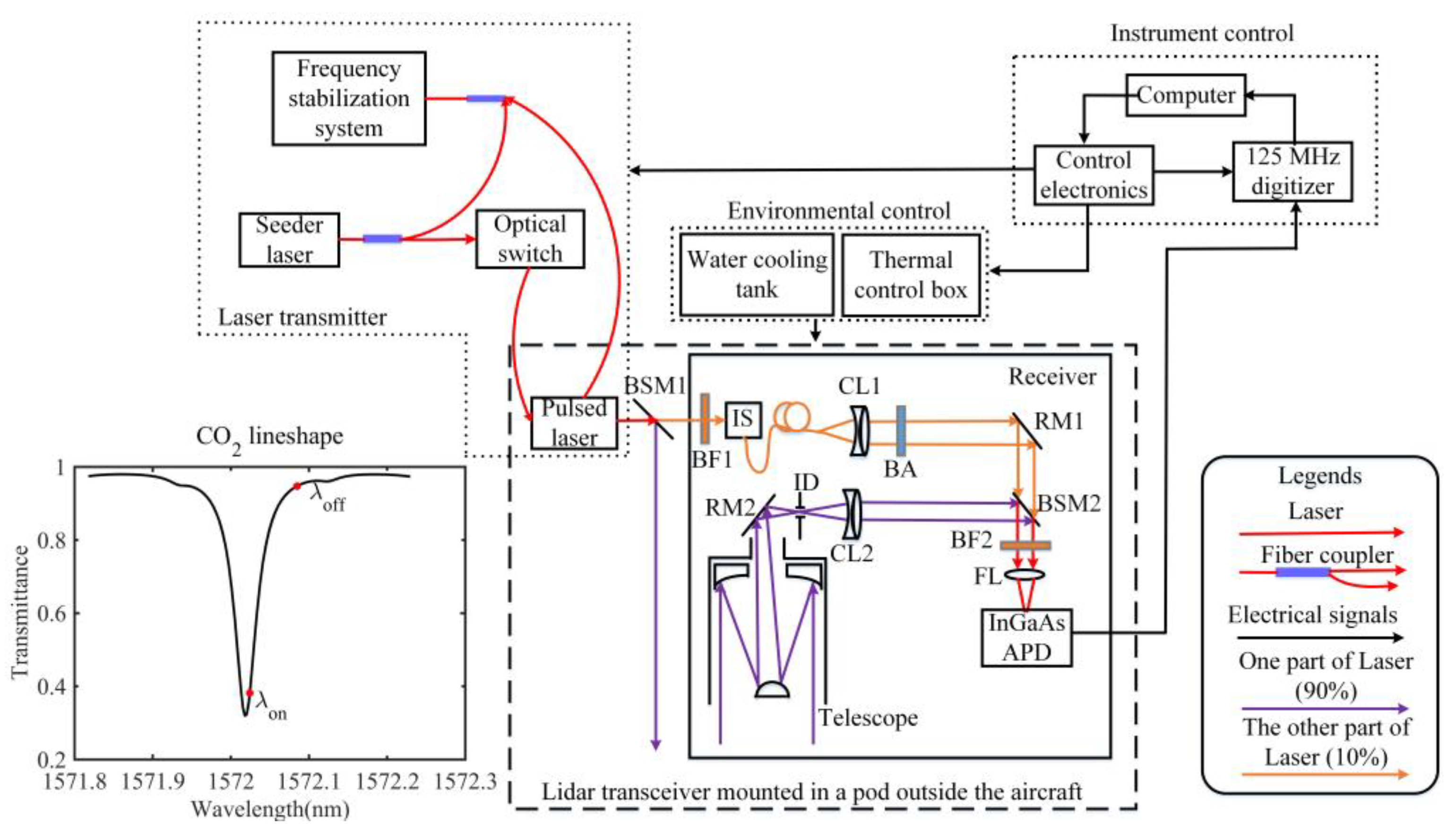
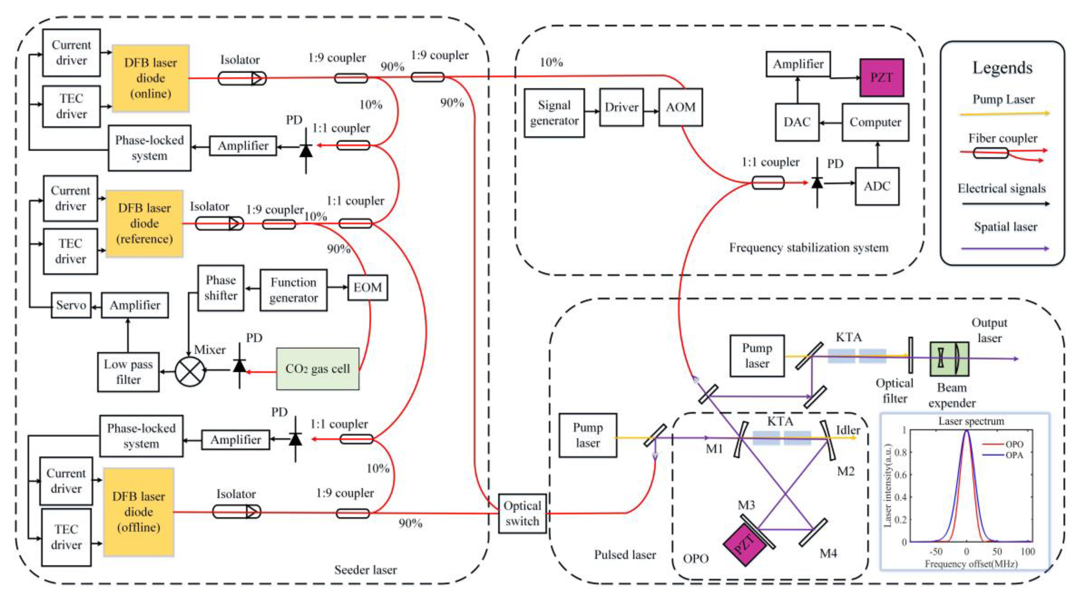
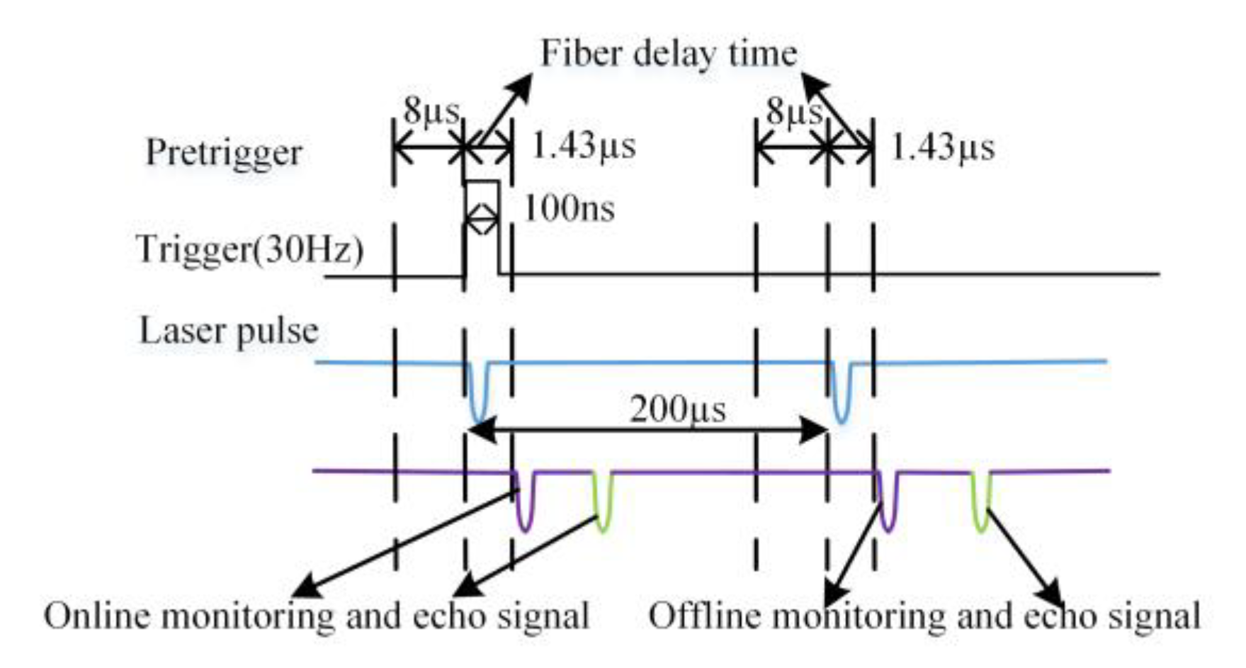
2. IPDA LIDAR Instrument and Principle

The schematic diagram and CO₂ transmittance line of the airborne IPDA LIDAR system are shown in Figure 1. The airborne IPDA LIDAR system consists of a laser transmitter, instrument control, environmental control, and LIDAR transceiver subsystem. The transceiver system consists of a pulsed laser, telescope, and avalanche photodiode (APD) detector, which are mounted in a pod outside the aircraft. The environmental control, instrument control, and frequency stabilization system are installed inside the aircraft, and they transmit information to the instruments in the pod through armored optical fibers and cables. The primary performance parameters of the airborne double-pulse 1.57-µm IPDA LIDAR system are listed in

Table 1. Primary parameters of airborne double-pulse 1.57 µm IPDA LIDAR system.

Parameters	Value	Parameters	Value
Online wavelength	1572.024 nm	Pressure of CO2 gas cell	70 mbar
Offline wavelength	1572.085 nm	Receiver optical efficiency	0.3797
Pulse energy (on/off)	6/3 mJ	Estimated flight altitude	8 km
Pulse width (on/off)	17 ns	Telescope diameter	150 mm
Pulse separation	200 µs	Field of view	1 mrad
Frequency stability (RMS)	2.7 MHz	Detector type	IAG350H1D
Repetition frequency	30 Hz	Responsivity	0.94 A/W
Beam divergence	0.62 mrad	NEP	64 $\mathrm{fw}/\sqrt{Hz}$
Pulse spectral linewidth (OPA)	30 MHz	Excess noise factor	3.2 (@M = 10)
Emission optical efficiency	0.8955	Data acquisition	125 MS/s
Optical path of CO2 gas cell	12.9 m	Optical filter bandwidth	0.45 nm

.

The laser transmitter subsystem consists of a seeder laser, frequency stabilization system, pulsed laser, and several optical components, as shown in Figure 2. The distributed-feedback (DFB) laser diode (LD) serves as a reference laser, and its wavelength is locked in the center of the CO₂ line at 1572.0179 nm using the external frequency modulation technique [20]. The reference laser passes through the isolator, and then it is divided into two parts with a 1:9 coupler: 90% of the reference laser is used to stabilize its own frequency, and the rest is used to offset lock the wavelength of the online and offline laser. Next, 90% of the reference laser is modulated by a fiber-coupled electro-optic modulator (EOM) driven by a function generator. Then, the modulated laser is reflected and absorbed many times in the CO₂ gas absorption cell and then output. The wavelength can be precisely locked in the CO₂ absorption center by using the long path CO₂ absorption gas cell, which is the core element of reference frequency stabilization. The CO₂ absorption gas cell is a multipass astigmatism Herriott cell with a compact size of Φ 100 × 80 mm. The pressure, temperature, and optical path were optimized to 70 mbar, 308.15 K, and 12.9 m, respectively [21]. Finally, the InGaAs photodiode (PD) detects the transmitted laser beam and generates a voltage signal. The phase delay produced by the phase shifter compensates for the unequal delay between the local oscillator and the PD output signal. The output signal of the detector and the local oscillator signal after compensation pass through the mixer then through the low-pass filter and amplifier and generate the error signal proportional to the deviation of the laser frequency from the center of the CO₂ line. The loop servo feeds the error signal back to DFB LD. The error signal is used to identify the absorption peak by changing the working temperature and adjusting the injection current fast locking frequency through the proportional-integral network. The online and offline DFB LD are locked to the reference laser at 1572.024 and 1572.085 nm by the optical phase-locked loop (OPLL) of the phase-locked system [22]. The OPLL technology and experimental laboratory results of the seeder laser have been reported by Du et al. [23]. In eight hours, the root mean square (RMS) of the frequency shift can be suppressed to around 50 kHz in an average time of 0.1 s [23], which meets the requirement of IPDA LIDAR experiment that the laser frequency stability of seeder is below 300 kHz.

Only 10% of the online and offline laser is used to stabilize its own frequency by offset-frequency-locked to the reference laser. Then, 81% of the online laser and 90% of the offline laser are switched by an optical switch at an interval of 200 µs and a frequency of 30 Hz. The online/offline laser is injected into the OPO cavity from M1 and then amplified by the pump laser through a group of KTA crystals. The idling light is output from M2. The amplified laser is reflected by M2, M3, and M4. Most of the laser is injected into the optical parametric amplifier (OPA) after M1 reflection. A small amount of laser transmitted through M1 is coupled with the 1:1 optical coupler. Moreover, the frequency of 9% of online laser frequency is shifted by 400 MHz from the AOM to reduce the overlap between the intensity envelope of the optical pulse and the beat signal of the optical heterodyne. The shifted laser received by PD is combined with the amplified laser by the 1:1 optical coupler, and then the beat frequency signal is analyzed using the ADC and computer. The analyzed error signal represents the difference between drifted frequency and 400 MHz. Then error signal was converted to a voltage applied to the PZT actuator by the DAC. The position of M3 can be changed slightly by PZT so that the OPO cavity length and the seeder laser frequency can be matched stably. The frequency fluctuation of the frequency-stabilized OPO is 0.29 MHz (RMS), with the Allan deviation being less than 20 kHz for an averaging time of more than 3 s [19]. The results meet the experimental requirements of IPDA LIDAR with pulsed laser frequency stability less than 0.3 MHz (RMS). The once-amplified frequency stabilized laser is further amplified by the OPA to achieve the required energy. Finally, the laser is output through the optical filter and beam expander. The laser spectra output by OPO and OPA are shown in bottom right corner of Figure 2, with linewidth of 24 MHz and 30 MHz respectively.

The transceiver subsystem consists of an integrating sphere (IS), Cassegrain telescope, iris diaphragm (ID), and several optical components. BSM1 divides the transmitted laser beam into two parts. One part is used for energy monitoring. It passes through the bandpass filter1 (BF1) into the IS. BF1 avoids the influence of other stray light, and the IS reduces the influence of the pointing jitter on the monitoring error. Then, it is coupled into a multimode fiber after diffuse reflection from the IS surface. After being collimated by the collimating lens1 (CL1), it goes through the beam attenuator (BA), and is reflected by the reflecting mirror1 (RM1). Finally, it goes through beam splitter mirror2 (BSM2), and bandpass filter2 (BF2), and is focused by a focusing lens (FL) on an InGaAs APD. The signal detected through this optical path is called the “monitoring signal”, which represents the change in laser energy. The other part is transmitted into the atmosphere, where it is reflected by a hard target. The echo laser is collected by the Cassegrain telescope with a diameter of 150 mm and is reflected by reflecting mirror2 (RM2). It then goes through the ID, and is collimated by the collimating lens2 (CL2). After reflected by BSM2, it goes through BF2, and is finally focused by the FL on the same detector. The signal detected through the optical path is called the “echo signal”. The instrument control subsystem consists of control electronics, a 125-MHz digitizer, and a computer. The environmental control subsystem is composed of a water-cooling tank and thermal control box. The detailed descriptions of the instrument control subsystem and the environmental control subsystem are shown in Section 3.

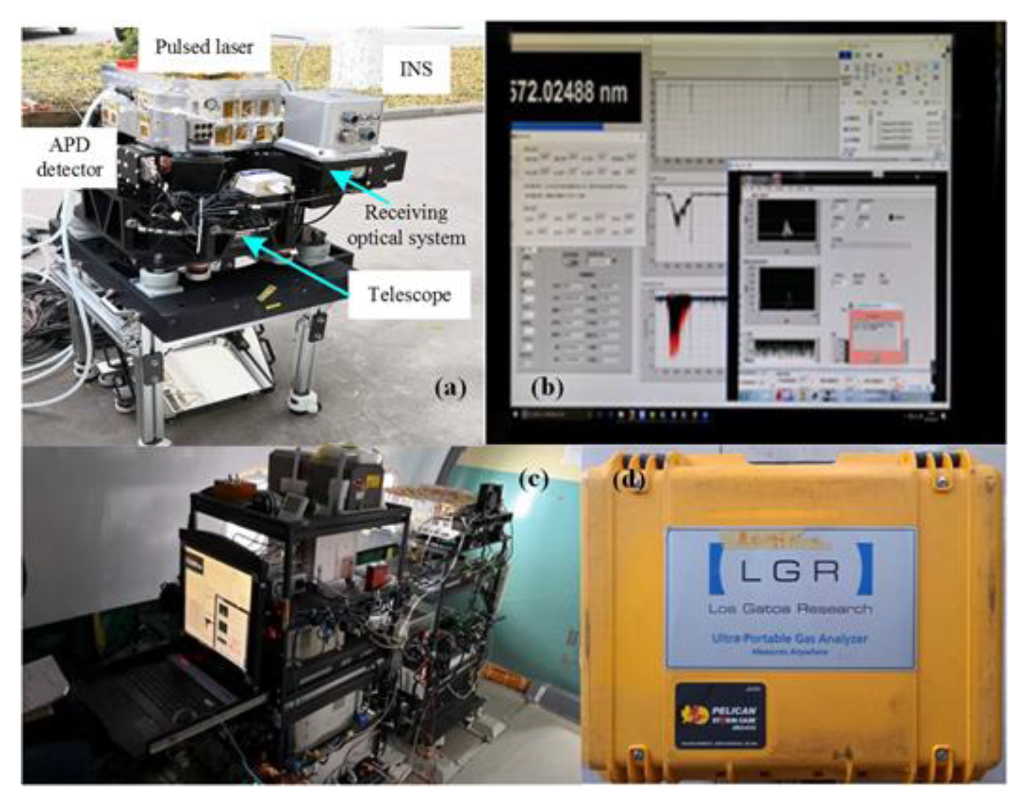
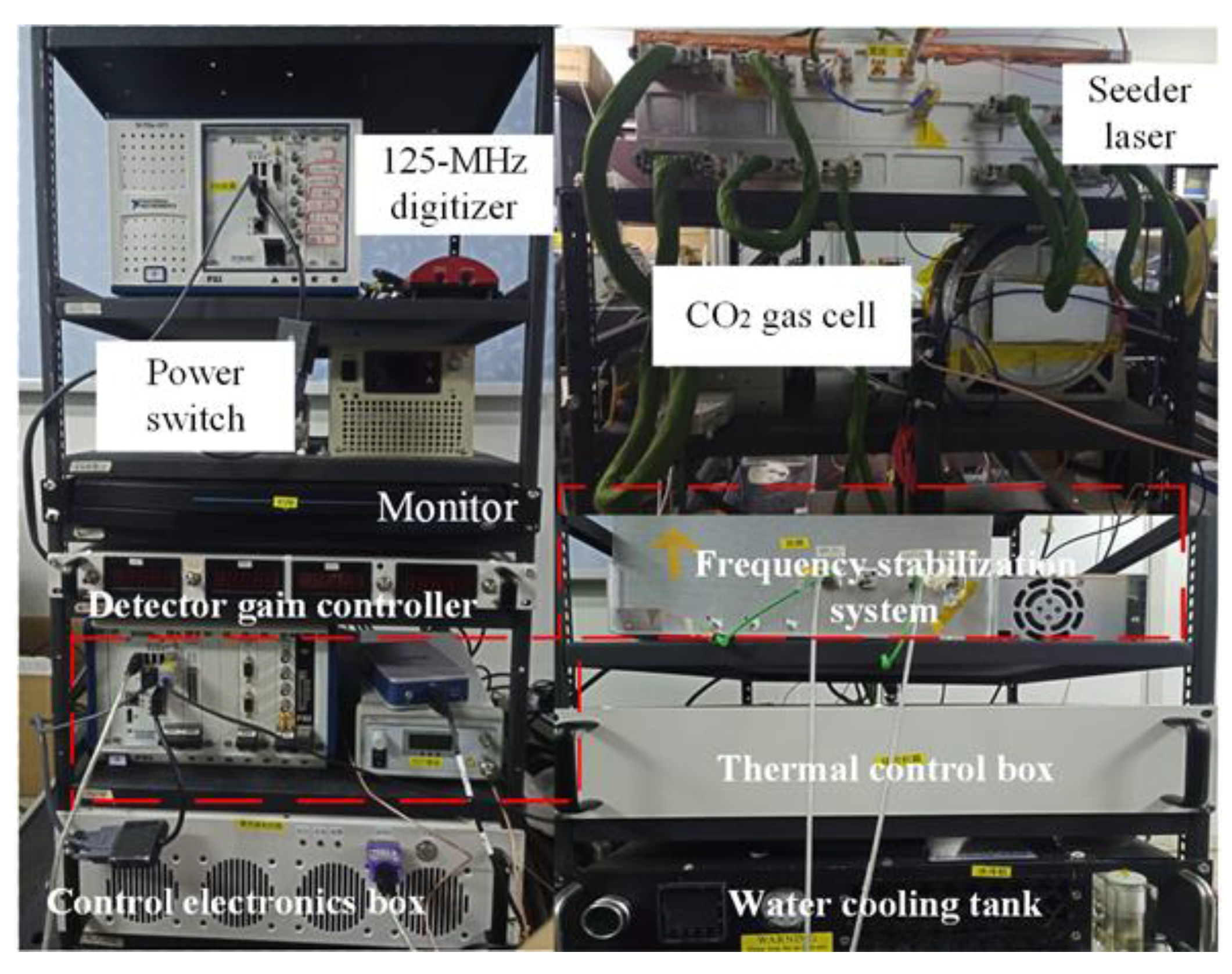
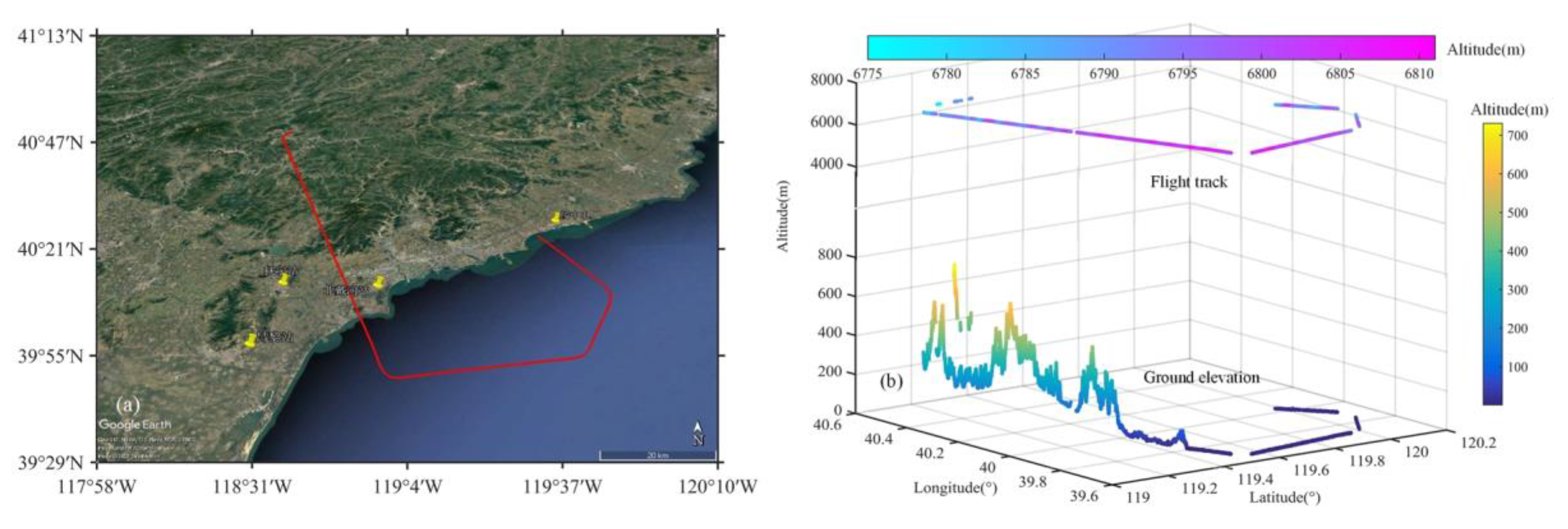
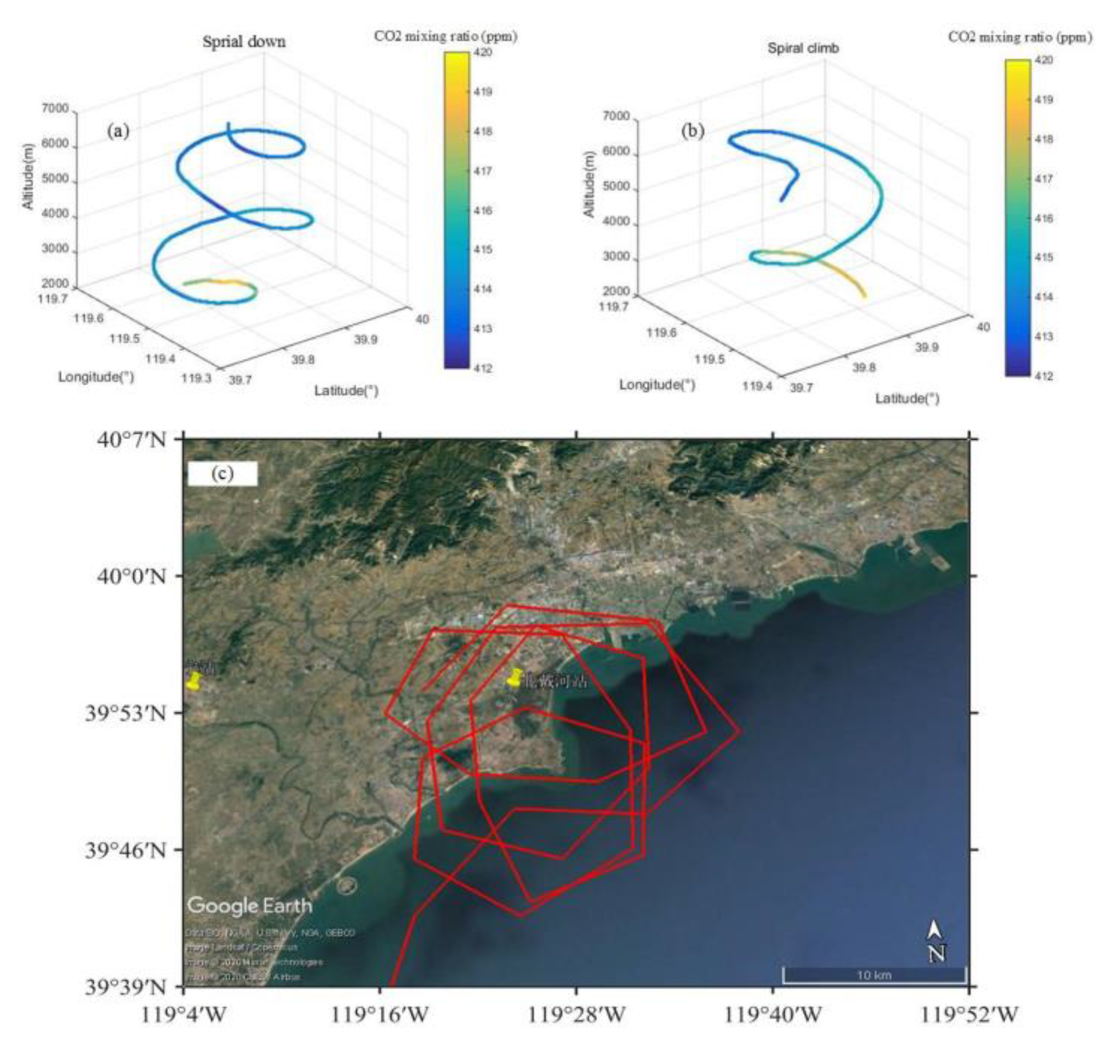
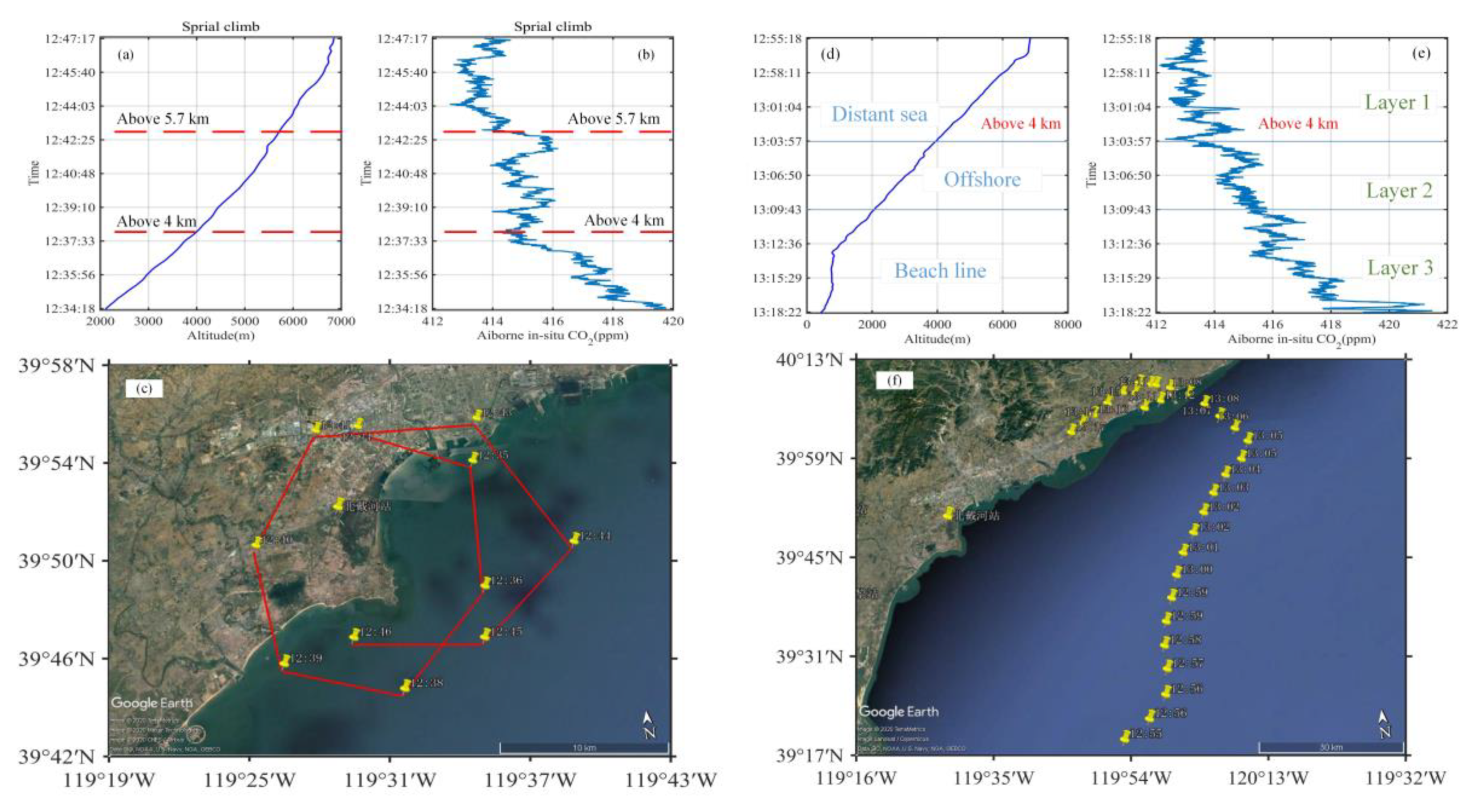
3. The Airborne Campaign

In spring 2019, the first airborne operation of the IPDA LIDAR system was launched in Shanhaiguan. The photographs of the IPDA LIDAR system are shown in Figure 3. As shown in Figure 3a, the transceiver system, consisting of a pulsed laser, telescope, and APD detector, is installed in a pod outside the aircraft. The INS is installed on the same base beside the laser transmitter, and the y-axis marked on the INS points in the same direction as the aircraft’s forward direction. The time, altitude, and posture information acquired by the INS and GPS are tagged in front of the LIDAR signals every 0.05 s. The control interface for laser frequency monitoring, laser frequency stabilization, and data acquisition is shown in Figure 3b. The environmental control, control electronics, seeder laser and frequency stabilization system shown in Figure 3c are installed inside the aircraft and transmit information to transceiver system in the pod through armored optical fibers and cables. Figure 4 shows the detail description of Figure 3c. The in-situ instrument shown in Figure 3d is an ultra-portable gas analyzer, which is based on Los Gatos Research’s patented technology (the fourth generation cavity enhanced absorption technique). Here, it has been calibrated with the gas standard of meteorological organization, and the uncertainty was within 0.1 ppm. To avoid the influence of the aircraft exhaust, the gas collection port is set in front of the aircraft engine.

When flying at 7 km, the temperature of the external environment is almost minus thirty degrees Celsius. Although hot air is ejected from the aircraft through the pipes, the temperature in the pod is still close to zero degrees Celsius. By monitoring and adjusting the temperature of the water-cooling tank and thermal control box, the environmental control subsystem can keep the instruments in the pod at a normal operating temperature. The water-cooling tank operates from water circulation and internal thermistor, which is used to keep the temperature of the pulsed laser constant. The thermal control box operates from the heating plates and thermistors attached to transceiver system. The instrument control subsystem consists of control electronics, a 125-MHz digitizer, and a computer. As the nerve center of the laser transmitter, control electronics provides power, controls the timing sequence of the laser output, and controls the startup sequence of the laser transmitter, together with the upper computer software. It also supplies power to the InGaAs APD detector and many other instruments. The 125-MHz digitizer converts the analog signal from the APD detector to the digital signal, which is collected and stored by the computer. The computer also works in tandem with the corresponding software to collect and store information on INS, GPS, online laser frequency, temperature, humidity, and pressure.

The route of the airborne experiment across ocean, residential and mountain areas was designed. The purpose was to detect the changing trend of CO₂ concentration. The flight track across three different areas is shown in Figure 5a. The aircraft flew from the seaside to the ocean area around 35 km away from the coast. It then flew across the residential area toward the mountainous area. The flight altitude and corresponding ground elevation are shown in Figure 5b. The ground elevation was obtained by subtracting the projection of the laser pulse propagation path from the flight altitude in the z-axis direction of the local geographic coordinate system [16]. As Figure 5b shows, some data are missing from the flight track. Data loss is mainly caused by cloud cover and excessive roll angle, which hampers the path calculation of the laser. In this experiment, we mainly focused on the XCO₂ trend from the flight altitude to the ground. Therefore, the data reflected by the cloud or roll angle greater than five degrees have been removed.

4. Data Retrieval and Analysis

The timing relationship of four pulses received by the IPDA LIDAR system is shown in Figure 6. The interval time between the online and offline pulse is 200 µs, and the pulse pair repetition frequency is 30 Hz. To measure and correct the system bias in the data inversion processing, the pre-trigger time was set to 8 µs. A 300-µm-diameter multimode fiber was used to delay the time of 1.43 µs to avert the influence of stray light from mirrors on the energy monitoring signal. The peak position of the monitoring signal was fixed at 9.43 µs, with the position of the echo signal depending on the flight altitude and terrain. To save storage space, the signals within 80 µs after triggering are enough to receive echo signals. The online and offline signal are spliced when they are stored.

The received signals of the IPDA LIDAR system in different areas are shown in Figure 7. The monitoring signal is fixed at the same position while the position of the echo signal varies with different regions. Because the altitude of the mountainous and residential areas is higher than the sea level, the flight time from the aircraft to the mountainous and residential areas is shorter than the sea level.

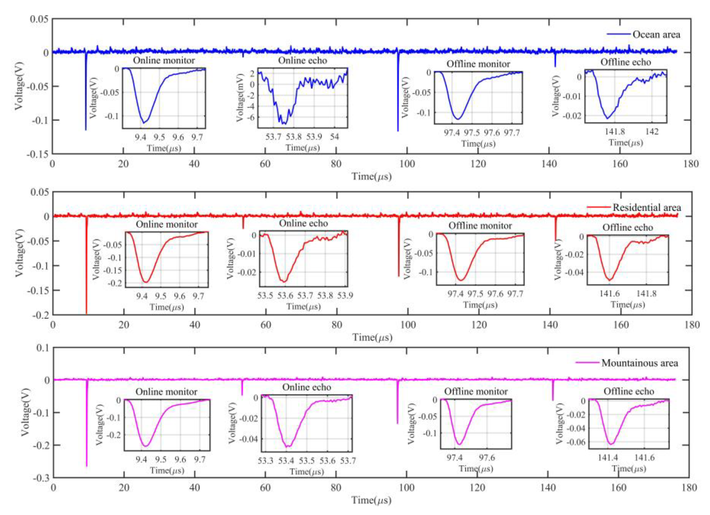
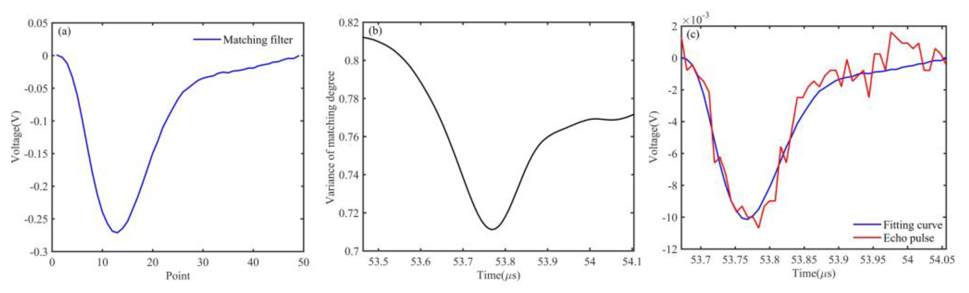
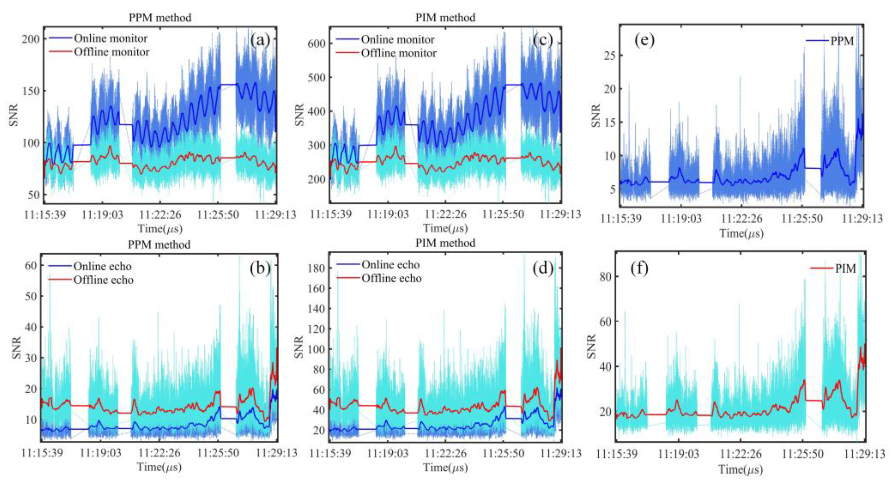
4.1. Extraction of the Weak Signal

According to Figure 7, the echo signal obtained in the ocean area is very weak, and its peak is disturbed by noise. It is difficult to identify the true peak position using the minimum value method (MVM) due to random noise. The matched-filter algorithm (MFA) is widely used to extract the echo signals of the seawater [24,25,26]. The matching moment is obtained by calculating the degree of matching between the echo signal and the matched filter. The degree of matching can be calculated by variance and expressed as [25]

$$D\left(t\right)=\frac{1}{N}{\displaystyle \sum }_{m=1}^N{\left[S\left(m\right)-W_R\left(m+t\right)\right]}^2,$$

(1)

where $D\left(t\right)$ is the variance and considered the index of the degree of matching, $S$ is the matched filter, $N$ is the length of the signal, $W_R$ is the echo signal, and $t$ is the offset. The following simulation verifies the effectiveness of the MFA.

The selected matched-filter in Figure 8a is a monitoring signal pulse with a high SNR, and the peak position is fixed and known. The variance between the echo signal and the matched filter is calculated by Equation (1). As shown in Figure 8b, the minimum position of the variance is the peak position of the echo signal, which is at 53.768 µs. After the peak position of the echo signal is obtained, the echo signal can be fitted using the matched filter. Figure 8c shows the comparison between the fitting curve obtained by the least square method and the original echo signal. The peak position obtained by the MVM is at 53.784 µs, and as Figure 8c shows, the peak position obtained by the MFA is different from MVM.

Besides the peak value, the difference between the two methods is not only in the peak position. The peak value identified by the MVM is not the true value disturbed by random noise but the true value plus the statistical bias. Using these two methods, the peak values of online and offline echo signals were obtained, as shown in Figure 9. The value of the statistical bias is from the peak values obtained by the MVM minus the peak values obtained by the MFA. The mean value of the statistical bias of the online and offline echo signals is 0.736 mV and 0.684 mV, respectively. When the signal amplitude is large, its noise disturbance is small. Therefore, the statistical bias of the offline signal is smaller than that of the online signal. For the online signal with a peak value of 10 mV, the influence of the statistical bias on it is around 7.36%. For the offline signal with a peak value of 20 mV, the influence of the statistical bias on it is around 3.42%. This effect is far beyond our requirement of 1 ppm inversion accuracy. When there is no strong wind and the sea surface is relatively calm, the echo signal is not widened by the terrain fluctuation. Therefore, it is reasonable to use the monitoring signal with a large SNR as the matched filter to calculate the peak position of the weak echo signal.

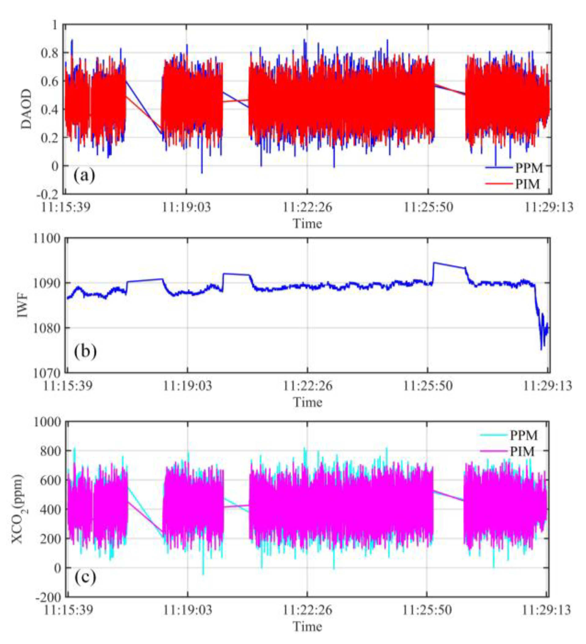
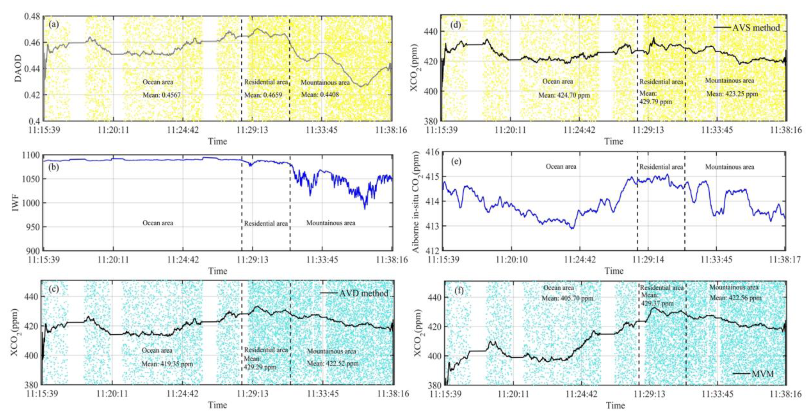
4.2. Data Processing and XCO₂ Retrievals

The changing trend of the received signals of the IPDA LIDAR system with the terrain and laser transmitter energy is shown in Figure 10. The changing trend of the monitoring signals reflects the changing trend of laser energy. In this airborne experiment, the LIDAR transceiver system was placed in the pod outside the aircraft, which, unfortunately, precluded the preheating of the instrument. It took a long time for the performance of the instruments to be stable after takeoff. In the process of balancing the temperature controlled by the environmental control system and the external environment, the laser energy of the online pulse continued rising, which took some time. The received power of the echo pulse varies greatly with different terrains due to different target reflectivity. From the changing trend of the ratio of the offline echo signal to offline monitoring signal, the reflectivity of land is 2–3 times that of the ocean, which is consistent with the reflectivity results of different targets [12,27,28]. The data in Figure 10 are taken from a route with relatively stable laser energy and a somewhat stable aircraft flight altitude, which is consistent with the route in Figure 5. The purpose of selecting this route across three different regions was to detect the changing trend of CO₂ concentration.

The monitoring powers of the online and offline pulses are represented by $P^{o{n}_0}$ and $P^{of{f}_0}$, respectively. The echo powers of the online and offline pulses are represented by $P^{on}$ and $P^{off}$, respectively. The IPDA single-path differential absorption optical depth (DAOD) of CO₂ can be expressed as [9,29]

$${\tau }_{C{O}_2}={{\displaystyle \int }}_{R_G}^{R_A}\Delta {\sigma }_{C{O}_2}\left(p\left(r\right),T\left(r\right)\right)N_{C{O}_2}\left(r\right)dr=\frac{1}{2}·ln\left(\frac{P^{off}·P^{o{n}_0}}{P^{on}·P^{of{f}_0}}\right).$$

(2)

where $\Delta {\sigma }_{C{O}_2}$ is the difference in absorption cross section between the online and offline wavelengths, $N_{C{O}_2}$ is the number density of the CO₂ molecules, $R_A$ is the altitude of airborne platform, and $R_G$ is the altitude of the hard target above sea level. When the APD detector receives the signal, the power of the signal can be converted to voltage by

$$V=P_P\ast {\Re }_v,$$

(3)

where ${\Re }_v$ is the voltage responsivity of the APD detector, which is a fixed value within the linear response range of the detector. $P_P$ is the power of signal. Hence, Equation (2) can be expressed as

$${\tau }_{C{O}_2}=\frac{1}{2}·ln\left(\frac{V_{off}·V_{o{n}_0}}{V_{on}·V_{of{f}_0}}\right).$$

(4)

In the airborne experiment, vertical path XCO₂ (in ppm) was given by

$$X_{C{O}_2}=\frac{{\tau }_{C{O}_2}}{2\times {10}^{-6}·IWF } ,$$

(5)

$$IWF={{\displaystyle \int }}_{R_G}^{R_A}\frac{N_A·p\left(r\right)·\Delta {\sigma }_{C{O}_2}\left(p\left(r\right),T\left(r\right)\right)}{RT\left(r\right)\left(1+X_{H_{2}O}\left(\mathrm{r}\right)\right)}dr,$$

(6)

where $N_A$ is Avogadro number, $R$ is gas constant, $p$ and $T$ are pressure and temperature profiles, $X_{H_{2}O}$ is the dry-air mixing ratio column of water vapor, and $IWF$ represents the integrated weighting function.

The profiles of temperature, humidity and pressure at different altitudes are shown in Figure 11, which are measured by an integrated sensor during the aircraft backspin stage. The IWF can be calculated using the profiles of temperature, humidity, and pressure, as well as Equation (6) and the high-resolution transmission molecular absorption (HITRAN) database [30]. These data are vital to the inversion of XCO₂.

In this study, the method of calculating DAOD using the peak value of pulse is called the “pulse peak method (PPM)”. The method to improve the SNR is called the “pulse integration method (PIM)”. Instead of using the peak value, the PIM uses the integrated value of the points on the pulse to calculate DAOD. When the response of the detector to the whole pulse of the signal is linear and the signal is not disturbed by noise, the inversion results of the PPM and PIM are consistent. However, due to the SNR of PIM is higher than that of PPM, the accuracy of PIM inversion results is higher. Therefore, the PPM is better in theory. In our experiment, the random noise followed Gaussian distribution, which is evident in Figure 12. When the points on the pulse are superposed, the sum continues following the Gaussian distribution of $N({\rho }^l,{({\epsilon }^l)}^2)$, where the mean and the standard deviation are

$${\rho }^l=\frac{1}{N}{{\displaystyle \sum }}_{k=1}^N{\alpha }_k^l,$$

(7)

$${\left({\epsilon }^l\right)}^2=\frac{1}{N^2}{{\displaystyle \sum }}_{k=1}^N{\left( {\sigma }_k^l\right)}^2,$$

(8)

where ${\alpha }_k^l$ is the value of each point on the pulse, and ${\sigma }_k^l$ is the standard deviation of each point. Hence, the SNR of the sum can be written as

$$SN{R}_{PIM}^l=\frac{{\rho }^l}{{\epsilon }^l}=\frac{{{\displaystyle \sum }}_{k=1}^N{\alpha }_k^l}{\sqrt{{{\displaystyle \sum }}_{k=1}^N{\left( {\sigma }_k^l\right)}^2}}.$$

(9)

Therefore, we can choose the number of points on the pulse to improve the SNR of each pulse. Figure 13 shows the pulse of the online echo signal and the change of the SNR in tandem with the number of points taken from the pulse. When taking six points before the peak value and seven points after the peak value, the SNR is maximum.

The echo signals in the ocean area are weaker than those in other areas. Therefore, the advantages of the PIM are illustrated when the data of the ocean area are analyzed. The SNR trend in the ocean area of the online and offline monitoring signals and the online and offline echo signals calculated by the PPM and PIM are shown in Figure 14a–d, respectively. Since the noise of each signal is uncorrelated, the total SNR can be expressed as

$$\frac{1}{SN{R}_{total}}=\sqrt{\frac{1}{SN{R}_{o{n}_0}^2}+\frac{1}{SN{R}_{of{f}_0}^2}+\frac{1}{SN{R}_{on}^2}+\frac{1}{SN{R}_{off}^2}},$$

(10)

where $o{n}_0$, $of{f}_0$, $on$, and $off$ represent the online and offline monitoring signals and the online and offline echo signals, respectively. The trend of the total SNR calculated by the PPM and PIM is shown in Figure 14e,f. The SNR calculated by the PIM is approximately 2–3 times of the PPM. Moreover, DAOD in the ocean area calculated by Equation (4) is shown in Figure 15a. The IWF in the ocean area calculated by Equation (6) is shown in Figure 15b and XCO₂ calculated by Equation (5) is shown in Figure 15c. The vibrations of DAOD and XCO₂ calculated by the PPM are larger than those of the PIM. Hence, we choose to use the PIM in the subsequent inversion process.

Many methods exist for the data inversion of XCO₂. Many researchers have discussed the advantages and disadvantages of the methods of “log before averaging” and “log after averaging” [23,24]. In this study, the scheme of averaging signals before log is called “AVS” while the scheme of computing the ratio of the mean DAOD and the mean IWF is called “AVD”. The XCO₂ calculated by the AVD method can be expressed as

$${\overline{X_{C{O}_2}}}^{AVD}=\frac{\langle {\tau }_{C{O}_2}\rangle }{\langle IWF\rangle },$$

(11)

where the triangular bracket notation denotes the arithmetic sample mean $\langle X\rangle =\frac{1}{N}{\sum }_{i=1}^N{X}_i$ of quantity $X$. XCO₂ calculated by the AVS method can be expressed as

$${\overline{X_{C{O}_2}}}^{AVS}=\frac{\frac{1}{2}·ln\left(\overline{V_r}\right)}{\langle IWF\rangle },$$

(12)

where $\overline{V_r}=\frac{\langle V_{off}\rangle ·\langle V_{o{n}_0}\rangle }{\langle V_{on}\rangle ·\langle V_{of{f}_0}\rangle }$ averages each signal before log.

The DAOD and IWF trends across the ocean, residential, and mountainous areas are shown in Figure 16a,b. In this study, the following results were retrieved by 1500 shoots sliding averages. The mean value of DAOD is 0.4567 in the ocean area, 0.4659 in the residential area, and 0.4408 in the mountainous area. The mean value of XCO₂ calculated using the AVD method is 419.35 ppm in the ocean area, 429.29 ppm in the residential area, and 422.52 ppm in the mountainous area, which is shown in Figure 16c. The mean value of XCO₂ calculated using the AVS method is 424.70 ppm in the ocean area, 429.79 ppm in the residential area, and 423.25 ppm in the mountainous area (see Figure 16d). The CO₂ concentration trend measured using airborne in-situ instrument at approximately 7 km is shown in Figure 16e. The mean value of XCO₂ calculated using the MVM is 405.70 ppm in the ocean area, 429.37 ppm in the residential area, and 422.56 ppm in the mountainous area (see Figure 16f). The XCO₂ values of the residential and mountainous areas retrieved by AVD, AVS, and MVM are almost the same, while the XCO₂ values of the ocean area retrieved by the three methods are quite different. As Figure 16e shows, the CO₂ concentration measured by the in-situ instrument of the residential area is higher than that of mountainous area and higher than that in the ocean area. Therefore, the inversion result of the AVS method in the ocean area is unreasonable. Figure 16e shows that the CO₂ concentration of the ocean area is higher than 413 ppm, rendering the MVM inversion result 405.70 ppm unreasonable. Moreover, compared with other methods, the XCO₂ trend inverted by AVD is more similar to the CO₂ concentration measured by the airborne in-situ instrument. Hence the AVD method is more suitable for our experiment. The average values of XCO₂ in the three areas are 419.35, 429.29, and 422.52 ppm respectively. The gradient of the residential and sea areas is 9.94 ppm, with that of the residential and mountainous areas being 6.77 ppm.

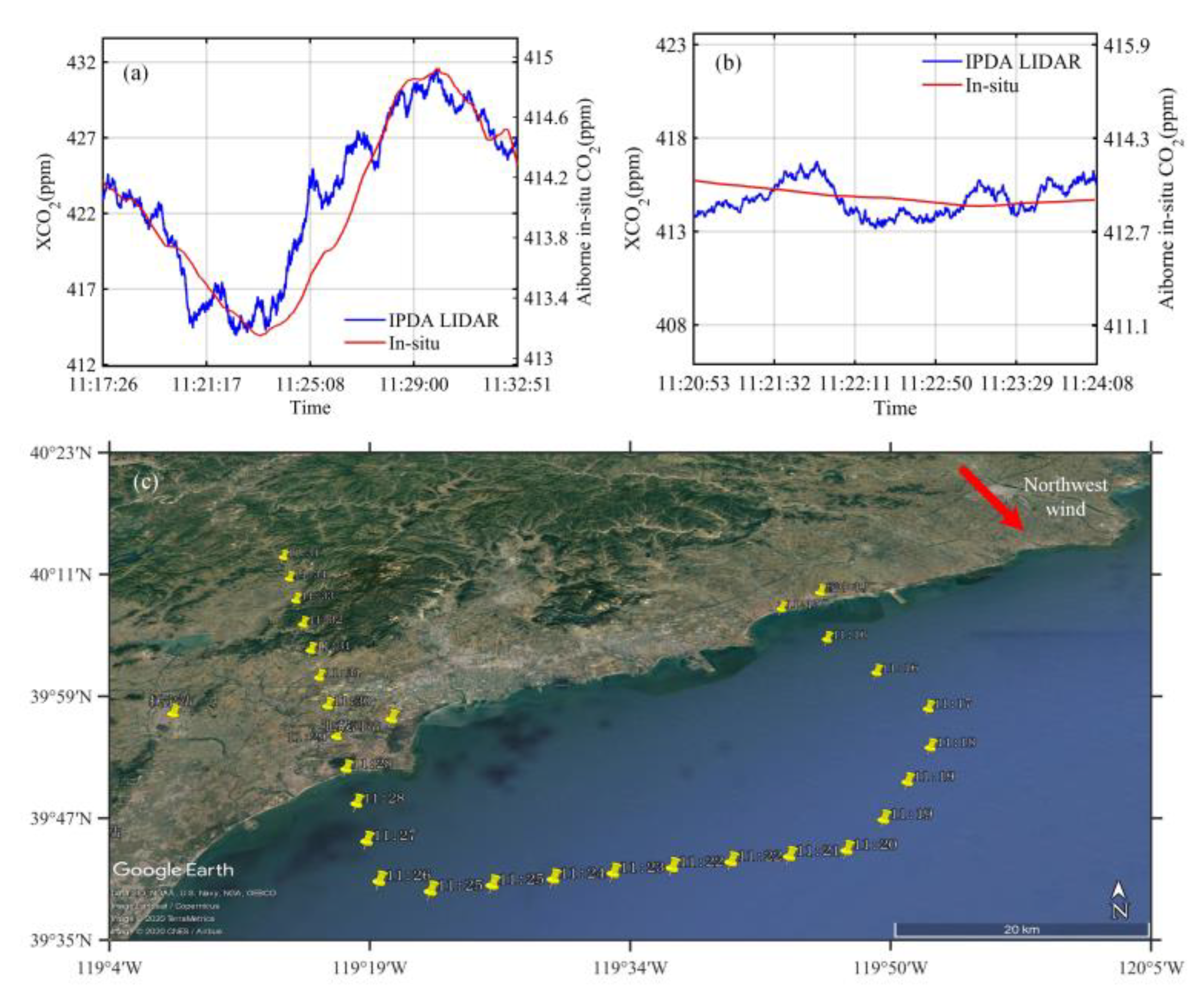
4.3. Comparisons of the IPDA LIDAR and In-Situ Instrument

A considerable amount of data was lost due to the large roll angle of the airplane and cloud during the experiment. To compensate for the time gap caused by data loss and better compare the inversion results of the IPDA LIDAR system with the changing trend of the in-situ measurement instrument, the XCO₂ value at a specific time is calculated by averaging the signal at the nearest time point from the time point. The XCO₂ measured by the IPDA LIDAR is a range average value that differs from the measurement by in-situ instrument realized at the airplane altitude. Therefore, the direct comparison between these two measurement methods is unreasonable. In this paper, we only compared the long-term change trend of XCO₂ measured by the IPDA LIDAR system and change trend of in-situ measurement instrument, which was evaluated the correlation coefficient between them. In addition, the XCO₂ retrieved by the IPDA LIDAR system is directly compared with CO₂ concentration measured by the in-situ instrument only in the steady stage of the open sea, which is justified in detail in the following analysis and discussion.

The comparison between the changing trend of XCO₂ retrieved by the IPDA LIDAR system and CO₂ concentration measured by the in-situ instrument in a long period is shown in Figure 17a. The correlation between them is 92% and the result illustrates the reliability of the changing trend of XCO₂ retrieved by the IPDA LIDAR system. On the other hand, the trend of XCO₂ retrieved by the IPDA LIDAR system is consistent with the wind direction (Northwest wind) of the day. In the process of flying from the residential area to the open sea, the XCO₂ gradually decreases with the increase of the distance away from the residential area. In the process of flying from the open sea to the residential area, the carbon dioxide concentration gradually increases with the decrease of the distance from the residential area. The steady stage of the open sea and the comparison between the IPDA LIDAR and in-situ instrument are shown in Figure 17b. As evident in Figure 17c, the route between 11:20 and 11:24 is 30 km away from the coast, which is less affected by the residential area and the CO₂ concentration is considered well-mixed. The mean value of XCO₂ retrieved by the IPDA LIDAR system between 11:20 and 11:24 is 414.69 ppm, with the standard deviation being 1.02 ppm. The mean value of CO₂ concentration measured by the in-situ instrument is 413.39 ppm. The bias between the XCO₂ retrieved by the IPDA LIDAR system and CO₂ concentration measured by the in-situ instrument in this period is 1.30 ppm.

5. Discussion

The echo signal obtained in the ocean area is very weak, and its peak value is disturbed by noise. The peak value retrieved by the MVM exhibited the statistical bias. For the online signal with a peak value of 10 mV, the influence of the statistical bias is around 7.36%. The MFA is applied to the extraction of the peak position and peak value, and the statistical deviation is eliminated. The range of total SNR calculated by the PPM is 6–14, and that calculated by the PIM is 20–42. Therefore, the SNR calculated by the PIM is approximately 2–3 times that of the PPM. The MFA and PIM plays an important role in the extraction and calculation of weak signals. The XCO₂ inversion results calculated by AVD, AVS and MVM are compared. The mean values of XCO₂ in the three regions are shown in

Table 2. The mean values of XCO₂ in three areas calculated by AVD, AVS and MVM.

Inversion Method	Ocean Area	Residential Area	Mountainous Area
AVS	424.70 ppm	429.79 ppm	423.25 ppm
AVD	419.35 ppm	429.29 ppm	422.52 ppm
MVM	405.70 ppm	429.37 ppm	422.56 ppm

. The XCO₂ values of the residential and mountainous areas retrieved by AVD, AVS, and MVM are almost the same, while the XCO₂ values of the ocean area retrieved by the three methods are quite different. Compared with other methods, the XCO₂ trend inverted by AVD is more similar to the CO₂ concentration measured by the airborne in-situ instrument. Hence, the AVD method is more suitable for our experiment. On the other hand, the trend of XCO₂ retrieved by the IPDA LIDAR system is consistent with the wind direction (Northwest wind) of the day. In the process of flying from the residential area to the open sea, the XCO₂ gradually decreases with the increase of the distance from the residential area. In the process of flying from the open sea to the residential area, the carbon dioxide concentration gradually increases with the decrease of the distance from the residential area. The open sea where is less affected by the residential area is in a steady stage.

The problems existing in the comparison between the IPDA LIDAR and in-situ instrument are analyzed as follows. Due to the limitations of the local air traffic control (ATC) system, there is no dry-air volume mixing ratio profile of CO₂ during spiral descent to the ground from flight altitude of 7 km at a fixed location. As shown in Figure 18, we only obtained dry-air volume mixing ratio profile of CO₂ from flight altitude between 2 km and 7 km at a fixed location. In the process of climbing from flight altitude of 2 km to 7 km, dry-air volume mixing ratio profile of CO₂ at different altitudes was measured by in-situ measurement instrument, which is shown in Figure 19a–c. In the absence of CO₂ dry air volume mixing ratio profile of less than 2 km, it is difficult to compare CO₂ in Figure 19b with the inversion results of IPDA LIDAR. However, in the process of landing from flight altitude of 7 km to the airport, the dry-air volume mixing ratio profile of CO₂ at different altitudes was measured with in-situ measurement instrument, as shown in Figure 19d–f. As can be seen from Figure 19d,f, it successively passed through the open sea (25 km to 60 km away from the coast), offshore, beach line. As can be seen from Figure 19e, the CO₂ gas in layer 1 is well-mixed, the CO₂ gas in layer 2 gradually increases with the decrease of height and the process of approaching the coast, and the CO₂ gas in layer 3 suddenly increases near the ground.

The XCO₂ can be evaluated by the measured single point carbon dioxide concentration at different altitudes using the Equations (13) and (14).

$$XC{O}_2=\frac{{{\displaystyle \int }}_{h_1}^{h_2}vm{r}_{C{O}_2} \left(r\right)·WF\left(r\right)dr}{{{\displaystyle \int }}_{h_1}^{h_2}WF\left(r\right)dr},$$

(13)

$$WF\left(r\right)=\frac{N_A·p\left(r\right)·\Delta {\sigma }_{C{O}_2}\left(p\left(r\right),T\left(r\right)\right)}{RT\left(r\right)\left(1+X_{H_{2}O}\left(r\right)\right)}.$$

(14)

where $h_1$ and $h_2$ denote the altitude of ground and flight altitude of 7 km, respectively, $vm{r}_{C{O}_2}$ is the dry-air volume mixing ratio profile of CO₂, $p$ and $T$ are the pressure and temperature profiles given in Figure 11, $X_{H_{2}O}$ is the dry-air mixing ratio column of water vapor given in Figure 11. The result of XCO₂ calculated by Equations (13) and (14) is 414.83 ppm.

The location where the XCO₂ evaluated by in-situ instrument during aircraft descent are obtained is different from the IPDA LIDAR observation location, so it is impossible to directly compare them. However, in the process of aircraft descent, most of the tracks are above the sea area. Therefore, the result of 414.83 ppm is 0.14 ppm higher than the mean value of XCO₂ measured by the IPDA LIDAR between 11:20 and 11:24, which indicates that the deviation inversion result of the IPDA LIDAR is not very large. On the other hand, Figure 19b shows that the carbon dioxide gas in residential area and offshore area (within 10 km away from the coast shown by Figure 19c) is uneven over 4 km. However, Figure 19f shows that the CO₂ gas in layer 1 is well-mixed during the open sea (60 km to 25 km away from the coast with the altitude reduced from 7 km to 4 km). Therefore, it seems a reasonable assumption that the CO₂ concentration of the route 30 km away from the coast between 11:20 and 11:24 is considered well-mixed or the little difference between high altitude and low altitude. Furthermore, the direct comparison between the mean value of XCO₂ retrieved by the IPDA LIDAR system from 11:20 to 11:24 and single point carbon dioxide concentration measured by the in-situ instrument in same period seems possible. Figure 19f shows that the CO₂ gas in layer 2 and 3 is gradually increase with the decrease of height. Hence, it’s impossible to compare the IPDA LIDAR and in-situ instrument in residential and mountainous areas directly. The inversion results of the IPDA LIDAR also show that there is a big difference between the IPDA LIDAR and in-situ instrument in residential and mountainous areas. And in these areas, only the long-term change trend of XCO₂ measured by the IPDA LIDAR system and that of in-situ measurement instrument is compared, and the correlation coefficient between them is evaluated. This experiment provides us with experience in the campaign region selection and flight path design of the future airborne experiment for better comparison and verification.

In spring 2015, the GRSC conducted its first in-flight experiments for CO₂ and CH₄ observations on high altitude and long-range research aircraft (HALO). Amediek et al. identified and analyzed a power plant according to the changing trend of the measured CO₂ concentration and found that the measurement accuracy of a 20-km average value is less than 0.5% (about 2 ppm) [8]. In this paper, the long-term correlation between the changing trends of XCO₂ retrieved using the IPDA LIDAR system and CO₂ concentration measured by the in-situ instrument reached 92%. In the ocean area far away from the coast and less affected by the residential areas, the mean value of XCO₂ retrieved by the IPDA LIDAR system was 414.69 ppm, with the standard deviation being 1.02 ppm of a 7.5-km average value (calculated by 1500 shoots sliding averages, 30 Hz of repeat frequency and 150 m/s of flight speed). The reason for comparison with the GRSC is that they are similar in measurement principle and selected absorption line of R18. It can be seen from the comparison that the results of this airborne experiment are slightly better than their results.

The algorithm proposed in this paper is not suitable for all conditions. The MFA method of ocean’s weak signal extraction is not suitable for signal extraction in the mountainous area, mainly because the pulse is widened in the mountainous area. Tellier et al. has proposed the AVS method with higher accuracy, assuming that the change of signal obeys normal distribution in the average time [31]. However, in this experiment, the energy of the laser is not stable due to its need for the balance with the outside temperature. The inversion results showed that the AVD method is more suitable for this experiment. The accuracy of the inversion algorithm may be affected by the terrain, the trend of laser energy, the SNR, and the flight attitude. Therefore, the adaptability of the inversion algorithm needs to be further improved.

6. Conclusions

In this experiment, the 1.57-μm airborne double-pulse IPDA LIDAR system is developed for CO₂ measurement. In spring 2019, the first airborne campaign of the IPDA LIDAR system was conducted in Shanhaiguan. The flight path passed across the ocean, residential and mountainous areas. The transceiver system was mounted in a pot outside the aircraft. The environmental control, instrument control, and frequency stabilization system were installed inside the aircraft and transmitted information to the instruments in the pod using armored optical fibers and cables. During the experiment, the sensors for temperature, pressure, and humidity, the INS, and the GPS are integrated with the airborne IPDA LIDAR system to aid the inversion of XCO₂. Moreover, the in-situ UGGA instrument for CO₂ measurement was mounted near the IPDA LIDAR system. It was calibrated with gas standards of the meteorological organization, with its uncertainty being within 0.1 ppm. To avert the influence of the aircraft exhaust on the measurement accuracy, the gas collection port was set in front of the aircraft engine.

The echo signals were successfully received by the IPDA LIDAR system. The received power of the echo pulse varied greatly with different terrains due to different target reflectivity. From the changing trend of the ratio of the offline echo signal to offline monitoring signal, land reflectivity is 2–3 times of the ocean reflectivity. The echo signal obtained in the ocean area is very weak and its peak is disturbed by noise. The peak value retrieved by the MVM exhibited the statistical bias. For the online signal with a peak value of 10 mV, the influence of the statistical bias around 7.36%. The MFA is applied to the retrieval of the peak position and peak value to eliminate the statistical bias. When there is no strong wind and the sea surface is relatively calm, the echo signal is not widened by the terrain fluctuation. Thus, it is reasonable to use the monitoring signal with a large SNR as the matched filter for the calculation the peak position of the weak echo signal in the ocean area. Meanwhile, instead of using the PPM, the PIM is employed to improve the SNR. The number of points was chosen on the pulse to improve the SNR of each pulse. The change of the SNR of the online echo signal with the number of points taken from the pulse was analyzed. The SNR is maximum when six points were taken before the peak value and seven points after the peak value. The SNR calculated by the PIM is approximately 2–3 times that of the PPM following the analysis of the data of the ocean area. The vibrations of DAOD and XCO₂ calculated by the PPM are larger than the vibration of the PIM. Hence, we used the PIM in the inversion process. The three methods of AVD, AVS and MVM were compared with the inversion of XCO₂. The XCO₂ values of the residential and mountainous areas retrieved by the three methods were almost the same, while the XCO₂ values retrieved by the three methods are quite different. The CO₂ concentration measured by the in-situ instrument of residential area is higher than that of the mountainous area, with that of the mountainous area being higher than that of the ocean area. Moreover, the CO₂ concentration of the ocean area is higher than 413 ppm. However, the inversion result of the AVS method in the ocean area is higher than that in the mountainous area. The inversion result of the MVM in the ocean area is 405.70 ppm, which is much lower than the value measured by the in-situ instrument. Moreover, compared with other methods, the XCO₂ trend inverted by AVD is more similar to CO₂ concentration measured by the airborne in-situ instrument. Therefore, the AVD method is more suitable for our experiment.

To compensate for the time gap caused by data loss and better compare the inversion results of the IPDA LIDAR system with the changing trend of the in-situ measurement instrument, the XCO₂ value at a specific time is calculated by averaging the signal at the nearest time point from the time point. The long-term correlation between the changing trend of XCO₂ retrieved by the IPDA LIDAR system and CO₂ concentration measured by the in-situ instrument is 92%. In the ocean area far away from the coast and less affected by the residential area, the bias between the XCO₂ retrieved by the IPDA LIDAR system and CO₂ concentration measured by the in-situ instrument is 1.30 ppm, with the standard deviation being 1.02 ppm. The flight path passes across the ocean, residential, and mountainous areas, with the mean value of XCO₂ of the three areas are 419.35, 429.29, and 422.52 ppm, respectively. The gradient of the residential and ocean areas was 9.94 ppm, with the gradient of the residential and mountain areas being 6.77 ppm. Obvious gradients were noticeable in different regions.

References

1. Ehret, G.; Kiemle, C.; Wirth, M.; Amediek, A.; Fix, A.; Houweling, S. Space-borne remote sensing of CO2, CH4, and N2O by integrated path differential absorption lidar: A sensitivity analysis. Appl. Phys. B-Lasers O 2008, 90, 593–608. [Google Scholar] [CrossRef] [Green Version]
2. Kawa, S.R.; Mao, J.; Abshire, J.B.; Collatz, G.J.; Sun, X.; Weaver, C.J. Simulation studies for a space-based CO2 lidar mission. Tellus B 2010, 62, 759–769. [Google Scholar] [CrossRef]
3. Han, G.; Ma, X.; Liang, A.L.; Zhang, T.H.; Zhao, Y.N.; Zhang, M.; Gong, W. Performance Evaluation for China’s Planned CO2-IPDA. Remote Sens. 2017, 9, 768. [Google Scholar] [CrossRef] [Green Version]
4. Singh, U.N.; Refaat, T.F.; Ismail, S.; Davis, K.J.; Kawa, S.R.; Menzies, R.T.; Petros, M. Feasibility study of a space-based high pulse energy 2 mu m CO2 IPDA lidar. Appl. Opt. 2017, 56, 6531–6547. [Google Scholar] [CrossRef] [PubMed]
5. Han, G.; Xu, H.; Gong, W.; Liu, J.Q.; Du, J.; Ma, X.; Liang, A.L. Feasibility Study on Measuring Atmospheric CO2 in Urban Areas Using Spaceborne CO2-IPDA LIDAR. Remote Sens. 2018, 10, 985. [Google Scholar] [CrossRef] [Green Version]
6. Abshire, J.B.; Ramanathan, A.; Riris, H.; Mao, J.P.; Allan, G.R.; Hasselbrack, W.E.; Weaver, C.J.; Browell, E.V. Airborne Measurements of CO2 Column Concentration and Range Using a Pulsed Direct-Detection IPDA Lidar. Remote Sens. 2014, 6, 443–469. [Google Scholar] [CrossRef] [Green Version]
7. Refaat, T.F.; Singh, U.N.; Yu, J.R.; Petros, M.; Remus, R.; Ismail, S. Double-pulse 2-mu m integrated path differential absorption lidar airborne validation for atmospheric carbon dioxide measurement. Appl. Opt. 2016, 55, 4232–4246. [Google Scholar] [CrossRef]
8. Amediek, A.; Ehret, G.; Fix, A.; Wirth, M.; Budenbender, C.; Quatrevalet, M.; Kiemle, C.; Gerbig, C. CHARM-F-a new airborne integrated-path differential-absorption lidar for carbon dioxide and methane observations: Measurement performance and quantification of strong point source emissions. Appl. Opt. 2017, 56, 5182–5197. [Google Scholar] [CrossRef] [PubMed]
9. Du, J.; Zhu, Y.D.; Li, S.G.; Zhang, J.X.; Sun, Y.G.; Zang, H.G.; Liu, D.; Ma, X.H.; Bi, D.C.; Liu, J.Q.; et al. Double-pulse 1.57 mu m integrated path differential absorption lidar ground validation for atmospheric carbon dioxide measurement. Appl. Opt. 2017, 56, 7053–7058. [Google Scholar] [CrossRef]
10. Abshire, J.B.; Ramanathan, A.K.; Riris, H.; Allan, G.R.; Sun, X.L.; Hasselbrack, W.E.; Mao, J.P.; Wu, S.; Chen, J.; Numata, K.; et al. Airborne measurements of CO2 column concentrations made with a pulsed IPDA lidar using a multiple-wavelength-locked laser and HgCdTe APD detector. Atmos. Meas. Tech. 2018, 11, 2001–2025. [Google Scholar] [CrossRef] [Green Version]
11. Mao, J.P.; Ramanathan, A.; Abshire, J.B.; Kawa, S.R.; Riris, H.; Allan, G.R.; Rodriguez, M.; Hasselbrack, W.E.; Sun, X.L.; Numata, K.; et al. Measurement of atmospheric CO2 column concentrations to cloud tops with a pulsed multi-wavelength airborne lidar. Atmos. Meas. Tech. 2018, 11, 127–140. [Google Scholar] [CrossRef] [Green Version]
12. Amediek, A.; Fix, A.; Ehret, G.; Caron, J.; Durand, Y. Airborne lidar reflectance measurements at 1.57 mu m in support of the A-SCOPE mission for atmospheric CO2. Atmos. Meas. Tech. 2009, 2, 755–772. [Google Scholar] [CrossRef] [Green Version]
13. Yu, J.R.; Petros, M.; Singh, U.N.; Refaat, T.F.; Reithmaier, K.; Remus, R.G.; Johnson, W. An Airborne 2-mu m Double-Pulsed Direct-Detection Lidar Instrument for Atmospheric CO2 Column Measurements. J. Atmos. Ocean. Tech. 2017, 34, 385–400. [Google Scholar] [CrossRef]
14. Tong, J.C.; Qu, Y.; Suo, F.; Zhou, W.; Huang, Z.M.; Zhang, D.H. Antenna-assisted subwavelength metal-InGaAs-metal structure for sensitive and direct photodetection of millimeter and terahertz waves. Photonics Res. 2019, 7, 89–97. [Google Scholar] [CrossRef]
15. Liang, Y.; Fei, Q.L.; Liu, Z.H.; Huang, K.; Zeng, H.P. Low-noise InGaAs/InP single-photon detector with widely tunable repetition rates. Photonics Res. 2019, 7, A1–A6. [Google Scholar] [CrossRef]
16. Zhu, Y.D.; Liu, J.Q.; Chen, X.; Zhu, X.P.; Bi, D.C.; Chen, W.B. Sensitivity analysis and correction algorithms for atmospheric CO2 measurements with 1.57-mu m airborne double-pulse IPDA LIDAR. Opt. Exp. 2019, 27, 32679–32699. [Google Scholar] [CrossRef]
17. Wirth, M.; Fix, A.; Mahnke, P.; Schwarzer, H.; Schrandt, F.; Ehret, G. The airborne multi-wavelength water vapor differential absorption lidar WALES: System design and performance. Appl. Phys. B-Lasers O 2009, 96, 201–213. [Google Scholar] [CrossRef] [Green Version]
18. Fix, A.; Budenbender, C.; Wirth, M.; Quatrevalet, M.; Amediek, A.; Kiemle, C.; Ehret, G. Optical Parametric Oscillators and Amplifiers for Airborne and Spaceborne Active Remote Sensing of CO2 and CH4. Lidar Technol. Tech. Meas. Atmos. Remote Sens. VII 2011, 8182. [Google Scholar] [CrossRef] [Green Version]
19. Chen, X.; Zhu, X.L.; Li, S.G.; Ma, X.H.; Xie, W.; Liu, J.Q.; Chen, W.B.; Zhu, R. Frequency Stabilization of Pulsed Injection-Seeded OPO Based on Optical Heterodyne Technique. Chin. Phys. Lett. 2018, 35, 024201. [Google Scholar] [CrossRef]
20. Wang, A.Q.; Meng, Z.X.; Feng, Y.Y. Widely tunable laser frequency offset locking to the atomic resonance line with frequency modulation spectroscopy. Chin. Opt. Lett. 2018, 16. [Google Scholar] [CrossRef]
21. Mu, Y.J.; Du, J.; Yang, Z.G.; Sun, Y.G.; Liu, J.Q.; Hou, X.; Chen, W.B. Design and simulation of a biconic multipass absorption cell for the frequency stabilization of the reference seeder laser in IPDA lidar. Appl. Opt. 2016, 55, 7106–7112. [Google Scholar] [CrossRef] [PubMed]
22. Wei, C.H.; Yan, S.H.; Jia, A.A.; Luo, Y.K.; Hu, Q.Q.; Li, Z.H. Compact phase-lock loop for external cavity diode lasers. Chin. Opt. Lett. 2016, 14. [Google Scholar] [CrossRef] [Green Version]
23. Du, J.; Sun, Y.G.; Chen, D.J.; Mu, Y.J.; Huang, M.J.; Yang, Z.G.; Liu, J.Q.; Bi, D.C.; Hou, X.; Chen, W.B. Frequency-stabilized laser system at 1572 nm for space-borne CO2 detection LIDAR. Chin. Opt. Lett. 2017, 15, 031401. [Google Scholar]
24. Luchinin, A.G. Complex modulation of airborne lidar light pulse: The effects of rough sea surface and multiple scattering. Proc. SPIE. 2012, 8532. [Google Scholar] [CrossRef]
25. Liu, M.G.; Yan, H.; Chen, W.B.; Wang, Y.X.; Hou, X.; Shi, X.G.; Huang, T.C.; Zhang, Y.F. Adaptive Depth Extraction Algorithm for Ocean Lidar. Chin. J. Lasers 2018, 45, 277–284. [Google Scholar]
26. Wei, X.F.; Chong, J.S.; Zhao, Y.W.; Li, Y.; Yao, X.N. Airborne SAR Imaging Algorithm for Ocean Waves Based on Optimum Focus Setting. Remote Sens. 2019, 11, 564. [Google Scholar] [CrossRef] [Green Version]
27. Disney, M.I.; Lewis, P.E.; Bouvet, M.; Prieto-Blanco, A.; Hancock, S. Quantifying Surface Reflectivity for Spaceborne Lidar via Two Independent Methods. IEEE Trans. Geosci. Remote 2009, 47, 3262–3271. [Google Scholar] [CrossRef]
28. Kiemle, C.; Kawa, S.R.; Quatrevalet, M.; Browell, E.V. Performance simulations for a spaceborne methane lidar mission. J. Geophys. Res.-Atmos. 2014, 119, 4365–4379. [Google Scholar] [CrossRef] [Green Version]
29. Refaat, T.F.; Singh, U.N.; Yu, J.R.; Petros, M.; Ismail, S.; Kavaya, M.J.; Davis, K.J. Evaluation of an airborne triple-pulsed 2 mu m IPDA lidar for simultaneous and independent atmospheric water vapor and carbon dioxide measurements. Appl. Opt. 2015, 54, 1387–1398. [Google Scholar] [CrossRef]
30. Gordon, I.E.; Rothman, L.S.; Hill, C.; Kochanov, R.V.; Tan, Y.; Bernath, P.F.; Birk, M.; Boudon, V.; Campargue, A.; Chance, K.V.; et al. The HITRAN2016 molecular spectroscopic database. J. Quant. Spectrosc. Radiat. 2017, 203, 3–69. [Google Scholar] [CrossRef]
31. Tellier, Y.; Pierangelo, C.; Wirth, M.; Gibert, F.; Marnas, F. Averaging bias correction for the future space-borne methane IPDA lidar mission MERLIN. Atmos. Meas. Tech. 2018, 11, 5865–5884. [Google Scholar] [CrossRef] [Green Version]
Figure 1. The schematic diagram of the airborne IPDA LIDAR system. BSM1, beam splitter mirror 1; BF1, bandpass filter 1; IS, integrating sphere; CL1, collimating lens 1; BA, beam attenuator; RM1, reflecting mirror 1; RM2, reflecting mirror 2; ID, iris diaphragm; CL2, collimating lens 2; BF2, bandpass filter 2; FL, focusing lens; APD, avalanche photodiode.
Remotesensing 12 01999 g001
Figure 2. Composition and operation schematic diagram of the laser transmitter. TEC, thermoelectric cooler; DFB, distributed-feedback; PD, photodiode, EOM, electro-optic modulator; AOM, acoustic-optic modulator; OPO, optical parametric oscillator; ADC, analog-digital converter; DAC, digital-analog converter; PZT, piezoelectric transducer; KTA, potassium titanyl arsenate. Note: There is only one PZT in the figure; however, it has been placed in different position to facilitate the drawing of the line from the amplifier to the PZT.
Remotesensing 12 01999 g002
Figure 3. Photographs of the IPDA LIDAR system. (a) The transceiver system mounted in a pod outside the aircraft. (b) The control interfaces of some instruments. (c) The environmental control, control electronics, seeder laser and frequency stabilization system are installed inside the aircraft. (d) The in-situ instrument for CO2 measurement is mounted inside the aircraft.
Remotesensing 12 01999 g003
Figure 4. Detail description of Figure 3c. The 125-MHz digitizer, power switch, monitor, detector gain controller, control electronics box, seeder laser, CO2 gas cell, frequency stabilization system, thermal control box, and water cooling tank were installed in two cabinets inside the aircraft.
Remotesensing 12 01999 g004
Figure 5. (a) The flight track across three different areas. (b) The flight altitude and corresponding ground elevation.
Remotesensing 12 01999 g005
Figure 6. Timing relationship of the airborne IPDA LIDAR system.
Remotesensing 12 01999 g006
Figure 7. The received signals of the IPDA LIDAR system over the ocean, mountainous and residential areas.
Remotesensing 12 01999 g007
Figure 8. (a) A high SNR monitoring signal pulse as matching filter. (b) The variance between the echo signal and the matched filter. (c) The comparison between the fitting curve and the original echo signal.
Remotesensing 12 01999 g008
Figure 9. (a) The peak values of the online echo signal obtained by the MVM. (b) The peak values of the online echo signal obtained by the MFA. (c) The statistical bias of the online echo signal. (d) The peak values of the offline echo signal obtained by the MVM. (e) The peak values of the offline echo signal obtained by the MFA. (f) The statistical bias of the offline echo signal.
Remotesensing 12 01999 g009
Figure 10. The trend of the received signals by the IPDA LIDAR system changing with the terrain and energy of the laser transmitter.
Remotesensing 12 01999 g010
Figure 11. The profiles of temperature, humidity, and pressure measured using the integrated sensor installed outside the aircraft during the spiral-down stage.
Remotesensing 12 01999 g011
Figure 12. Noise distribution characteristics during the flight experiment in the long-term statistical results and its Gaussian fitting curve.
Remotesensing 12 01999 g012
Figure 13. (a) The pulse of the online echo signal. (b) The change of the SNR with the number of points taken from the pulse.
Remotesensing 12 01999 g013
Figure 14. (a) The SNR trend in the ocean area of the online and offline monitoring signals calculated by the PPM. (b) The SNR trend of the online and offline echo signals calculated by the PPM. (c) The SNR trend in the ocean area of the online and offline monitoring signals calculated by the PIM. (d) The SNR trend in the ocean area of the online and offline echo signals calculated by the PIM. (e) The total SNR trend calculated by the PPM. (f) The total SNR trend calculated by the PIM.
Remotesensing 12 01999 g014
Figure 15. (a) The DAOD trend in the ocean area calculated by the PPM and PIM. (b) The IWF trend in the ocean area. (c) The XCO2 trend in the ocean area calculated by the PPM and PIM.
Remotesensing 12 01999 g015
Figure 16. (a) The DAOD trend across the ocean, residential, and mountainous areas. (b) The IWF trend. (c) The XCO2 trend calculated using the AVD method. (d) The XCO2 trend calculated using the AVS method. (e) The CO2 concentration trend measured by the airborne in-situ instrument at approximately 7 km. (f) The XCO2 trend of the calculated using the minimum value method.
Remotesensing 12 01999 g016
Figure 17. (a) The comparison between the changing trend of XCO2 retrieved by the IPDA LIDAR system and CO2 concentration measured by the in-situ instrument in a long period. (b) The comparison in the steady stage of the ocean area. (c) The flight route and the corresponding time are helpful for analyzing the inversion results.
Remotesensing 12 01999 g017
Figure 18. The single point dry-air volume mixing ratio of CO2 at different altitudes measured by in situ measurement instrument from flight altitude of 2 km to 7 km at a fixed location.
Remotesensing 12 01999 g018
Figure 19. (ac) The dry-air volume mixing ratio profile of CO2 at different altitudes was measured with in-situ measurement instrument in the process of climbing from flight altitude of 2 km to 7 km. (df) The single point carbon dioxide concentration at different altitudes measured by in-situ measurement instrument in the process of landing from flight altitude of 7 km to the airport.
Remotesensing 12 01999 g019