Letter

Toronto Water Vapor Lidar Inter-Comparison Campaign

1
Meteorological Research Division, Environment and Climate Change Canada, Toronto, ON M3H-5T4, Canada
2
Centre for Research in Earth and Space Science, York University, Toronto, ON M3J 1P3, Canada
3
Vaisala Oyj, 01670 Vantaa, Finland
*
Author to whom correspondence should be addressed.
Remote Sens. 2020, 12(19), 3165; https://doi.org/10.3390/rs12193165
Submission received: 31 August 2020 / Revised: 21 September 2020 / Accepted: 23 September 2020 / Published: 27 September 2020
(This article belongs to the Special Issue Advances in Atmospheric Remote Sensing with Lidar)

Abstract

:
This study presents comparisons between vertical water vapor profile measurements from a Raman lidar and a new pre-production broadband differential absorption lidar (DIAL). Vaisala’s novel DIAL system operates autonomously outdoors and measures the vertical profile of water vapor within the boundary layer 24 h a day during all weather conditions. Eight nights of measurements in June and July 2018 were used for the Toronto water vapor lidar inter-comparison field campaign. Both lidars provided reliable atmospheric backscatter and water vapor profile measurements. Comparisons were performed during night-time observations only, when the York Raman lidar could measure the water vapor profile. The purpose was to validate the water vapor profile measurements retrieved by the new DIAL system. The results indicate good agreement between the two lidars, with a mean difference (DIAL–Raman) of 0.17 ± 0.14 g/kg. There were two main causes for differences in their measurements: horizontal displacement between the two lidar sites (3.2 km) and vertical gradients in the water vapor profile. A case study analyzed during the campaign demonstrates the ability for both lidars to measure sudden changes and large gradients in the water vapor’s vertical structure due to a passing frontal system. These results provide an initial validation of the DIAL’s measurements and its ability to be implemented as part of an operational program.

Graphical Abstract

1. Introduction

Vertical profile measurements of water vapor are an essential meteorological observation, particularly with respect to numerical weather prediction (NWP) and global climate modeling [1,2,3]. Techniques to acquire measurements of the vertical profile of atmospheric water vapor continuously throughout a 24 h period are under active development. A new cost-effective instrument for continuous and comprehensive high spatial- and temporal-resolution profiling of water vapor within the boundary layer was investigated in this study.
Compared to radiosondes and passive remote sensing instruments (e.g., microwave radiometers) for profiling atmospheric water vapor, lidar-based technologies have the advantage of providing higher temporal and vertical resolution observations continuously. The two primary lidar techniques for water vapor profiling are differential absorption lidar (DIAL) and Raman lidar. Raman lidars, which make use of Raman scattering, are a mature technology and are commonly used for measurements of atmospheric gases such as water vapor [4,5]. DIAL systems utilize the difference between laser wavelengths centered on and off a water vapor absorption line to measure the water vapor mixing ratio (WVMR) [6]. They have been used to measure several trace gases, including water vapor, deployed as ground-based [7,8,9,10,11,12,13], airborne [14,15], and proposed for space-based [16] platforms, such as those in the NASA Langley DIAL program [17]. Most Raman lidars, such as the one used in this study, cannot take measurements of water vapor during the day. DIAL systems, however, can operate 24 h a day and do not require an on-site reference, making them ideal for operational deployment.
Recently, the performance of an earlier prototype DIAL system, developed by Vaisala, was evaluated by comparing it to coincident observations from a Raman lidar, radiosonde, and an atmospheric emitted radiance interferometer at the Southern Great Plains (SGP) site [18]. Previous inter-comparisons of the same system were performed in Germany, Finland, and Hong Kong, all demonstrating excellent measurement reliability [19,20]. Vaisala’s DIAL system is capable of automated and continuous (24-h) vertical attenuated backscatter and water vapor profiling during all weather conditions (up to a thick cloud base), providing night- and day-time observations, which most Raman lidars are incapable of.
An updated pre-production model of the Vaisala DIAL system was acquired by Environment and Climate Change Canada (ECCC) and deployed to the Toronto-Downsview test field in June 2018. This system is intended for operational use either as a stand-alone system or as part of a larger network. It is vital to assess the accuracy of the new DIAL pre-production model, particularly in other regions where the DIAL has not operated such as a complex urban environment. Hence, night-time comparisons between the Vaisala DIAL and the York University Raman lidar were performed in this study to provide an initial validation of the DIAL’s measurements (a subsequent study providing a detailed evaluation of the DIAL’s performance in the Canadian Arctic will soon follow). Section 2 describes the York Raman lidar and the Vaisala DIAL systems. Section 3 provides initial results from the DIAL and comparisons between the two lidar systems during the field campaign. Conclusions are provided in Section 4.

2. Materials and Methods

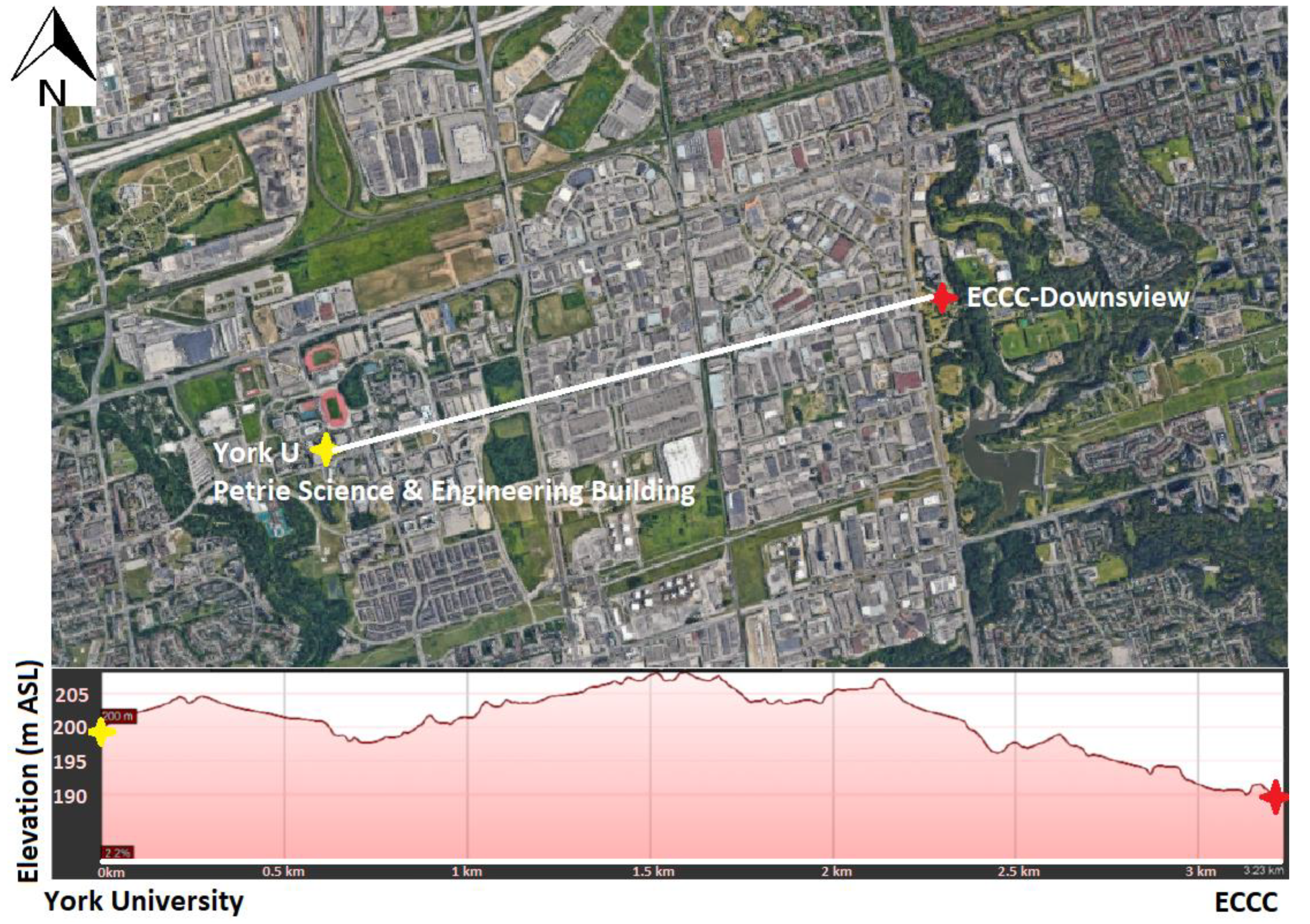
2.1. Field Campaign Site

The field campaign was conducted in northwestern Toronto, which is comprised of relatively flat terrain and low-, mid-, and high-rise residential, commercial, and industrial buildings. Several large parks and one major highway (highway 407) are located within the region, which is ~17 km north of Lake Ontario. Figure 1 shows the locations of the York University campus and the ECCC Downsview office, which are separated by 3.2 km. Fast-moving meteorological events such as passing fronts and deep-penetrating lake breezes, which are detectable by lidar-based technologies [21], frequently occur at the site during the summer and provide opportunities to measure sharp vertical gradients in the water vapor structure.
Observations were conducted with both lidars on each night from 29 June to 13 July 2018. The York Raman lidar viewed the atmosphere through a roof hatch in a laboratory on the fourth floor of the Petrie science and engineering building at York University. It was approximately 30 m higher in elevation than the DIAL lidar, which was deployed at ground-level in the ECCC-Downsview test field. Ideally, the two lidars would have been deployed side-by-side during the campaign, but this was not possible due to operational and logistical constraints at the time. The close proximity between York University and ECCC-Downsview nevertheless provided an excellent opportunity to perform comparisons between the two lidars.

2.2. York Raman Lidar
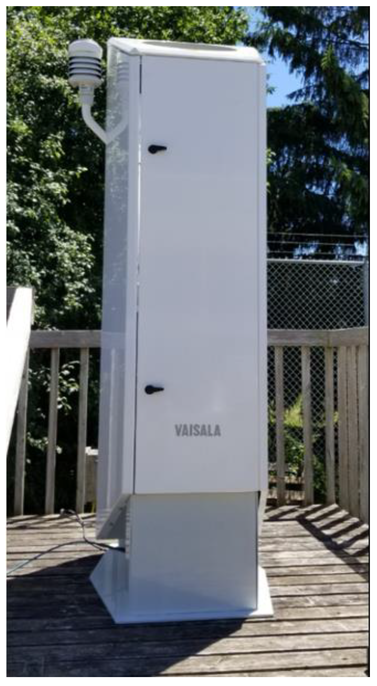
The York Raman lidar is a modification of an instrument that was previously developed for DIAL ozone measurements [22,23,24]. The transmitter was a Q-switched Nd:YAG laser with 3rd harmonic generation that provided pulsed light at a wavelength of 355 nm. The backscattered light was collected with a 15 cm diameter off axis parabolic mirror. An adjustable field stop aperture, at the focal plane of the parabolic mirror, provided a conical field of view with a full angle of 1 mrad or less. An optical fiber collected the light at the field stop and delivered it to an arrangement where the optical signals at various wavelengths were separated using tilted interference filters having a bandwidth of less than 1 nm. The optical signals detected using photomultiplier tubes were recorded using simultaneous photon counting and analog to digital conversion (ADC). The photon counting was used for the Raman scattering signals at wavelengths of 387 nm (from Nitrogen) and 407 nm (from water vapor), while ADC was required for the strong elastic backscatter signals near the ground. The vertical sampling bin width was 7.5 m and the measurement integration period was 10 s (200 laser shots). The first step of the analysis to derive WVMR was to further average over 20-min periods to reduce the uncertainty. A vertical sliding boxcar average was applied over an interval of 67.5 m.
The water vapor mixing ratio was determined from the ratio of the backscatter signals at 407 nm and 387 nm, with correction for the different atmospheric transmittance at the two wavelengths. Calibration had previously been carried out by comparison with measurements of water vapor with radiosondes launched from Buffalo, New York. The aerosol extinction coefficient was also derived from the measurements of elastic backscatter at a wavelength of 355 nm using the algorithm of [25].

2.3. Vaisala DIAL

Vaisala developed a prototype DIAL system in the mid-2010s that is fully-automated and requires no operator intervention with the exception of basic routine maintenance. It was deployed to Germany, Finland, China, and the SGP for validation and inter-comparison field campaigns. Technical details about the system and the WVMR retrieval technique are provided in detail in [18]. The Vaisala DIAL system acquired by ECCC in the summer of 2018 is a new, updated model that is the pre-production commercial version. The system went through initial acceptance testing at Vaisala headquarters in Vantaa, Finland, in March 2018 before it was deployed to ECCC’s Downsview test field as shown in Figure 2. The DIAL conducted measurements continuously from 24 June to 25 July 2018 with no instrument downtime experienced.
As described in detail in [18], the Vaisala DIAL uses diode laser transmitters to produce eye-safe pulsed infrared laser radiation. Two separate wavelengths are transmitted and received; one wavelength (911.0 nm) that is strongly absorbed by water vapor (“online”) and another wavelength (910.6 nm) that is mostly not absorbed by water vapor (“offline”). The switching speed is ~15 Hz (approximately 65 ms, including measurement and switching time). The spectrum of the online laser overlaps multiple water vapor absorption lines; thus, to retrieve estimates of the WVMR, a broadband DIAL equation is obtained from the ratio of the background-subtracted and pulse-normalized online and offline signals. A unique solution to the broadband DIAL equation is obtained via an inversion method, providing the WVMR as a function of height [18,26].
The DIAL’s design includes two vertically-pointing measurement units (lasers) placed side-by-side, contained within a larger shelter, with a Vaisala CL-series ceilometer-type telescope [19,27]. The near-field unit is optimized for measurements from 50 to 400 m and the far-field unit is optimized for measurements from 300 to 3000 m; the mixing ratios from the two fields are merged between 300 and 400 m using a linearly increasing weight such that the weight for the far-field unit is 0% at 299 m and 100% at 401 m. For quality control purposes, only data above 90 m AGL was used in this study. Humidity profiles are generated using a 20-min running average output every minute. A Vaisala WXT534 present weather sensor mounted on the DIAL provides measurements of the surface relative humidity, which is integrated into the DIAL retrieval algorithm for establishing the WVMR value in the lowest altitude bin of the retrieval, below the first DIAL range gate, as described in [18].
Estimates of the uncertainty in the water vapor profile and maximum effective range are provided by the DIAL’s quality control algorithm and are based on a threshold value in the standard deviation of the water vapor profiles and the online-to-offline signal ratio over the 20 min averaging period, respectively (see [18] for more details). While many of the technical specifications of the prototype DIAL outlined in [18] are the same as the ECCC pre-production model, some minor improvements were made to the system as outlined in Table 1.

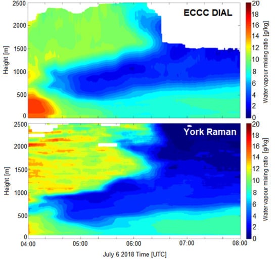
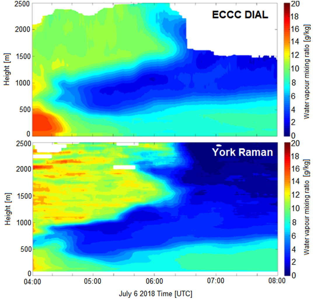
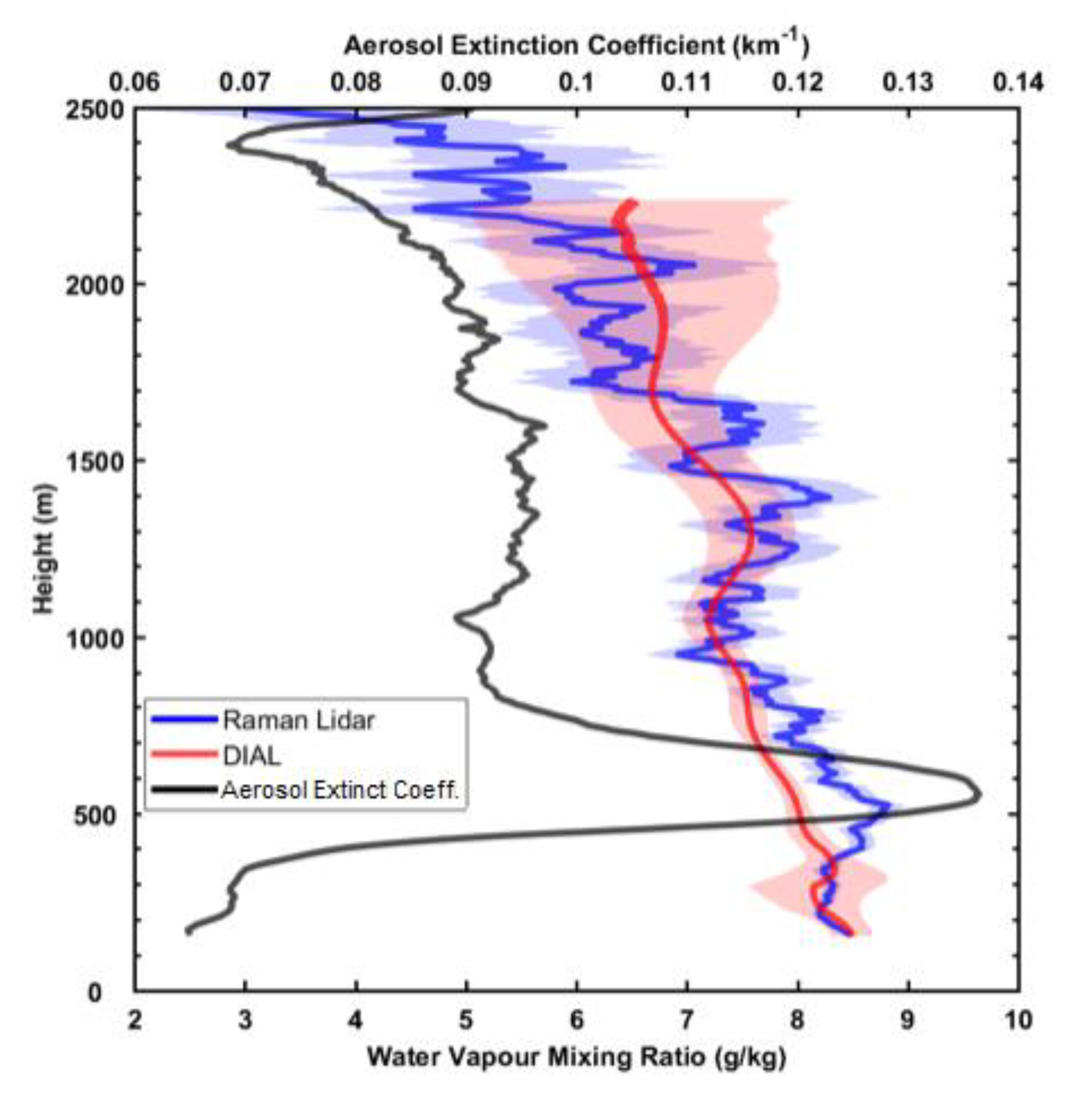
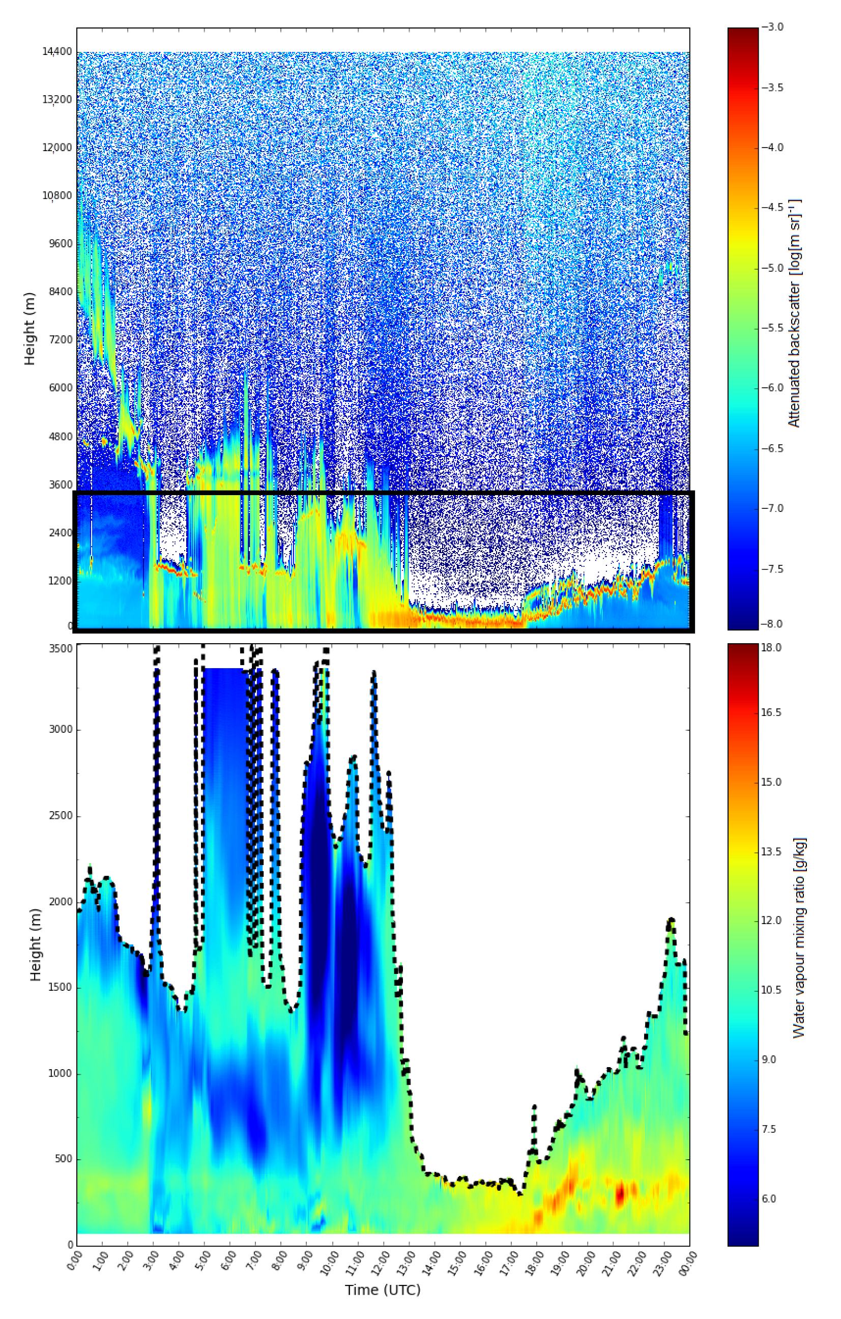
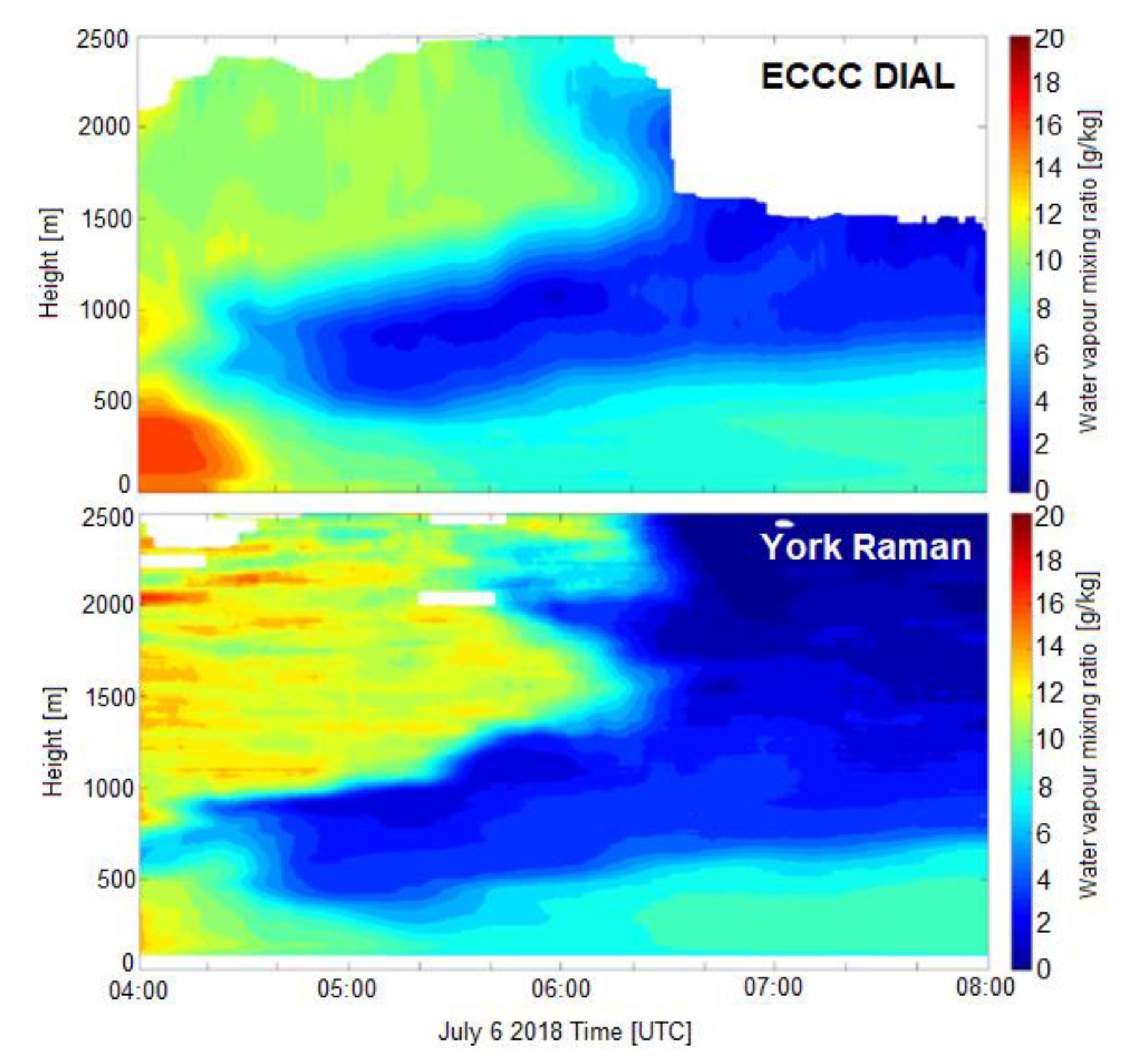
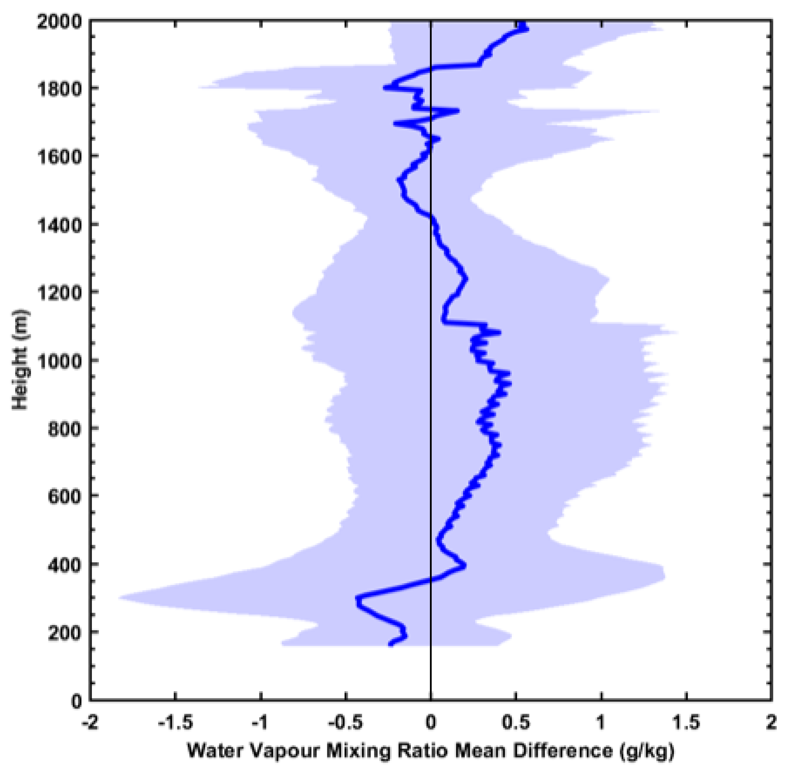
3. Results and Discussion

DIAL and Raman Lidar Comparisons

The night of July 10/11 provided a comparison between the Vaisala DIAL and York Raman lidars when the atmospheric conditions were not changing rapidly. Figure 3 shows a 20-min average of the water vapor mixing ratio profile measured with both lidars and the aerosol optical extinction coefficient measured by the Raman lidar during clear skies and constant meteorological conditions. There was a difference of ~0.8 g/kg in the water vapor mixing ratio where there was a distinct aerosol layer at around 600 m AGL, but the two lidar measurements were within the limits of uncertainty at all other heights up to the DIAL’s maximum effective range (2.23 km AGL) during this scan. During the campaign, the DIAL’s data availability, defined as the percentage of time for which the DIAL provided an observation at that height that passed its quality control (i.e., within its effective range), was ~100% below 500 m AGL, dropping only slightly up to 1400 m AGL. Roughly speaking, 1400 m AGL is typically near the average boundary layer height in Toronto during the summer months [21]. Above this height, the data availability for the DIAL dropped to <10% above 2.5 km AGL. Note that the DIAL has slightly lower maximum range during daytime operation due to solar background radiation [18].
Continuous observations from the DIAL during all weather conditions provide a novel dataset that can offer a unique glimpse into, for instance, the diurnal water vapor cycle and 24-h variability in the water vapor profile caused by meteorological events above Toronto. DIAL observations during rapidly-changing atmospheric conditions that included intermittent periods of heavy rain (8.6 mm total precipitation as measured at the Downsview test field site) on 22 July 2018 are shown in Figure 4 as an example that illustrates the DIAL’s 24-h profiling capability. The vertical attenuated backscatter profiles show varying cloud cover and other aerosols observed by the DIAL throughout the day. The DIAL’s backscatter observations match those from a Vaisala CL51 ceilometer co-located at the Downsview test field site (not shown). The most intense rainstorm ended at 14:00 UTC, which is shortly before local noon. Afterward, a significant increase in water vapor below 600 m AGL was observed due to evaporation during mostly clear skies and hot (26 °C) surface temperatures. The DIAL collected data before, during, and after precipitation, whereas most lidar systems shut down entirely during precipitation.
York Raman lidar measurements were acquired each night between 29 June and 13 July 2018. Eight separate nights (29 June, 4, 5, 8–12 July) were chosen for analysis and comparisons with the DIAL when there were no significant disruptions in the measurements due to rain or low clouds. The night of July 5–6 was a case in which the atmosphere changed rapidly with thunderstorms in the early evening followed by the passage of a cold front moving eastward after midnight. The lidar water vapor measurements indicate the front passed York University at ~04:10 UTC and ECCC-Downsview about 20 min later, at ~04:30 UTC. This was a worst-case scenario for the purposes of comparison from two separate locations; it demonstrates the sensitivity to vertical resolution and the challenges in comparing between two separate locations.
Both lidars were able to detect the passing cold front as a mass of dry air aloft at the time of the front’s passage, albeit offset by ~20 min, as shown in Figure 5. The differences between the two water vapor profiles occurred mainly where there were strong horizontal and vertical gradients (e.g., 500 to 700 m AGL). Another factor was that there was a difference in the elevation of the two locations; the air in the boundary layer near the surface approximately follows the contour of the terrain, but this is not the case at greater heights. The overall structure of the dry air mass as measured by the two lidars was almost identical. Mean night-time profiles on July 6 (04:00 to 08:00 UTC) had differences (DIAL–Raman) <1 g/kg whereas smaller night-time differences (<±0.25 g/kg up to 2 km AGL) were observed on nights when the atmospheric conditions did not change rapidly.
The average difference in the WVMR measurements between the two lidars for all 20-min profiles during the entire campaign (all eight nights) is shown in Figure 6. The mean difference (DIAL–Raman) between the two lidars was 0.17 ± 0.14 g/kg. This indicates excellent agreement between the two lidars given the 3.2 km separation distance and is in close agreement with comparisons performed in the SGP by [18]. A negative bias below 500 m AGL was observed, indicating the DIAL is biased low near the surface and biased high elsewhere (for the most part) compared to the Raman lidar, which was also observed in [18]. The mean difference and standard deviation of the difference peaked around 350 m AGL, which is the region where the DIAL’s near- and far-field units overlap. An updated processing algorithm is in development by Vaisala and is expected to remedy this as well as the slight positive bias throughout the rest of the profile that is caused by an overestimation of the laser spectral width in the retrieval algorithm.

4. Conclusions

During the Toronto water vapor lidar inter-comparison campaign (29 June to 13 July 2018), comparisons of atmospheric water vapor measurements were made between the York University Raman lidar and Vaisala’s new pre-production DIAL system operated by ECCC. The York Lidar operated during the night at York University, while the DIAL operated throughout day and night during all weather conditions 3.2 km to the east at ECCC-Downsview for an extended period (24 June to 25 July 2018).
The goal of the campaign was to assess the new pre-production DIAL’s measurements of the vertical distribution of water vapor. It was found that the two lidar instruments provided measurements of water vapor that were within the range of uncertainty in their profile measurements and the uncertainty associated with the distance separating the two lidars. During the campaign, there were examples of nights with little variability (Figure 3) and nights with large variability (Figure 5) in the WVMR vertical structure. The lidars were able to detect sudden changes in the water vapor profile caused by fast-moving meteorological features, such as a passing cold front, demonstrating their ability to resolve the evolution of a distinct structure within the atmospheric boundary layer. Averaged over the entire campaign, the mean difference (DIAL–Raman) between the two lidars was 0.17 ± 0.14 g/kg, which is excellent considering their horizontal separation distance. A new processing algorithm (under development) is expected to reduce the overall bias in the DIAL’s profile.
There were two main causes for differences between the lidars: horizontal displacement between the two lidars (3.2 km) and vertical gradients (steep vertical gradients and the change in elevation between the two lidars). For the cold front case which exhibited large vertical gradients (Figure 5), a larger difference between the two lidars was expected due to the difference in their locations causing a ~20 min offset between the two lidars’ observations. These results demonstrate the ability of the DIAL system to be implemented as part of an operational system, particularly in an urban environment where radiosondes cannot be launched.
After the Toronto water vapor inter-comparison campaign ended and other tests with the DIAL system were completed, it was relocated to the Canadian Arctic Weather Science (CAWS) project’s Iqaluit supersite [27,28] in September 2018. The DIAL has remained at Iqaluit to this day, performing exceptionally well, collecting observations on a continuous basis in the harsh Arctic climate without any technical issues (100% up-time with the exception of power outages at the site). The DIAL’s high temporal and spatial observations in the Arctic will be used to investigate prolonged stratified wind and water vapor layers above the Iqaluit site [29], the diurnal water vapor cycle, perform side-by-side comparisons to radiosonde observations and a Raman water vapor lidar co-located at the site for a detailed instrument validation study, and for NWP model verification and assimilation impact studies.

Author Contributions

Conceptualization, Z.M., J.W.; methodology, Z.M., J.W., and R.L.; formal analysis, Z.M., J.W., and N.S.; writing—original draft preparation, Z.M.; writing—review and editing, all. All authors have read and agreed to the published version of the manuscript.

Funding

This research received no external funding.

Acknowledgments

Special thanks to Michael Harwood, Robert Reed, Reno Sit, and Jason Iwachow for their help with deploying instrumentation. All DIAL data products are produced by ECCC and are available via obrs.ca or upon request. All Raman lidar data products are produced by York University and are available upon request.

Conflicts of Interest

The instrument manufacturer had no role in the design of the study; in the collection, analyses, or interpretation of data; in the writing of the manuscript, and in the decision to publish the results.

References

  1. Dessler, A.E.; Zhang, Z.; Yang, P. Water vapor climate feedback inferred from climate fluctuations, 2003–2008. Geophys. Res. Lett. 2008, 35, L20704. [Google Scholar] [CrossRef] [Green Version]
  2. Joe, P.; Melo, S.; Burrows, W.; Casati, B.; Crawford, R.; Deghan, A.; Gascon, G.; Mariani, Z.; Milbrandt, J.; Strawbridge, K. The Canadian Arctic Weather Science Project: Introduction to the Iqaluit Site. Bull. Am. Meteorol. Soc. 2019, 101. [Google Scholar] [CrossRef]
  3. Weaver, D.; Strong, K.; Schneider, M.; Rowe, P.M.; Walker, C.; Sioris, K.A.; Mariani, Z.; Uttal, T.; McElroy, C.T.; Vomel, H. Intercomparison of atmospheric water vapour measurements at a Canadian High Arctic site. Atmos. Meas. Tech. 2017, 10, 2851–2880. [Google Scholar] [CrossRef] [Green Version]
  4. Melfi, S.H. Remote measurements of the atmosphere using Raman scattering. App. Opt. 1972, 11, 1605–1610. [Google Scholar] [CrossRef] [PubMed]
  5. Whiteman, D.N. Examination of the traditional Raman lidar technique II Evaluating the ratios for water vapor and aerosols. Appl. Opt. 2003, 42, 2593. [Google Scholar] [CrossRef] [PubMed] [Green Version]
  6. Bosenberg, J. Ground-based differential absorption lidar for water-vapor and temperature profiling: Methodology. Appl. Opt. 1998, 37, 3845–3860. [Google Scholar] [CrossRef] [PubMed]
  7. Karapuzikov, A.; Malov, A.N.; Sherstov, I.V. Tunable TEA CO2 laser for long-range DIAL lidar. IR Phys. Technol. 2000, 41, 77–85. [Google Scholar] [CrossRef]
  8. Godin-Bekmann, S.; Porteneuve, J.; Garnier, A. Systematic DIAL lidar monitoring of the stratospheric ozone vertical distribution at Observatoire de Haute-Provence (43.92°N, 5.71°E). J. Environ. Monit. 2002, 5, 57–67. [Google Scholar] [CrossRef] [PubMed]
  9. Kiemle, C.; Ehret, G.; Giez, A.; Davis, K.J.; Lenschow, D.H.; Oncley, S.P. Estimation of boundary layer humidity fluxes and statistics from airborne differential absorption lidar (DIAL). J. Geophys. Res. 1997, 102, 29189–29203. [Google Scholar] [CrossRef]
  10. Nehrir, A.; Repasky, K.S.; Carlsten, J.L.; Obland, M.D.; Shaw, J.A. Water vapour profiling using a widely tuneable amplified diode-laser based differential absorption lidar (DIAL). J. Atmos. Ocean. Tech. 2009, 26, 737–745. [Google Scholar] [CrossRef] [Green Version]
  11. Baron, P.; Ishii, S.; Mizutani, K.; Itabe, T.; Yasui, M. Profiling tropospheric water vapour with a coherent infrared differential absorption lidar: A sensitivity analysis. In Proceedings of the Lidar Remote Sensing for Environmental Monitoring XIII, Kyoto, Japan, 29 October–1 November 2012; Volume 8526, p. 85260D. [Google Scholar] [CrossRef]
  12. Spuler, S.M.; Repasky, K.S.; Morley, B.; Moen, D.; Hayman, M.; Nehrir, A.R. Field-deployable diode-laser-based differential absorption lidar (DIAL) for profiling water vapor. Atmos. Meas. Tech. 2015, 8, 1073–1087. [Google Scholar] [CrossRef] [Green Version]
  13. Imaki, M.; Tanaka, H.; Hirosawa, K.; Yanagisawa, T.; Kameyama, S. Demonstration of the 1.53-µm coherent DIAL for simultaneous profiling of water vapor density and wind speed. Opt. Express 2020, 28, 27078–27096. [Google Scholar] [CrossRef] [PubMed]
  14. Machol, J.; Ayers, T.; Schwenz, K.T.; Koenig, K.W.; Hardesty, R.M.; Senff, C.J.; Krainak, M.A.; Abshire, J.B.; Bravo, H.E.; Sandberg, S.P. Preliminary measurements with an automated compact differential absorption lidar for profiling water vapour. App. Opt. 2014, 45, 3110. [Google Scholar]
  15. Poberaj, G.; Fix, A.; Assion, A.; Wirth, M.; Kiemle, C.; Ehret, G. Airborne all-solid-state DIAL for water vapour measurements in the tropopause region: System description and assessment of accuracy. Appl. Phys. B 2002, 75, 165–172. [Google Scholar] [CrossRef]
  16. Gerard, E.; Tan, D.G.H.; Garand, L.; Wulfmeyer, V.; Ehret, G.; Di Girolamo, P. Major advances in humidity profiling from the water vapour lidar experiment in space (WALES). Bull. Am. Meteorol. Soc. 2004, 85, 237–252. [Google Scholar] [CrossRef] [Green Version]
  17. Browell, E.V.; Ismail, S.; Grant, W.B. (Differential absorption lidar (DIAL) measurements from air and space. Appl. Phys. B 1998, 67, 399–410. [Google Scholar] [CrossRef]
  18. Newsom, R.K.; Turner, D.D.; Lehtinen, R.; Münkel, C.; Kallio, J.; Roininen, R. Evaluation of a compact broadband differential absorption lidar for routine water vapor profiling in the atmospheric boundary layer. J. Atmos. Ocean. Technol. 2020, 37, 47–65. [Google Scholar] [CrossRef]
  19. Roininen, R.; Münkel, C. Results from Continuous Atmospheric Boundary Layer Humidity Profiling with a Compact DIAL Instrument. In Proceedings of the Eighth Symposium on Lidar Atmospheric Applications, Seattle, WA, USA, 23 January 2017; American Meteorologic Society: Boston, MA, USA, 2017; Volume 12.3. Available online: https://ams.confex.com/ams/97Annual/webprogram/Paper301717.html (accessed on 14 July 2020).
  20. Münkel, C.; Roininen, R. Results from continuous atmospheric boundary layer humidity profiling with a compact DIAL instrument. In Proceedings of the European Conference for Applied Meteorology and Climatology, Dublin, Ireland, 4–8 September 2017; European Meteorological Society: Berlin, Germany, 2017; Volume 525. [Google Scholar]
  21. Mariani, Z.; Dehghan, A.; Sills, D.M.; Joe, P. Observations of lake breeze events during the Toronto 2015 pan-American games. Boundary Layer Meteorol. 2018, 166, 113–135. [Google Scholar] [CrossRef]
  22. Seabrook, J.A.; Whiteway, J.A.; Staebler, R.M.; Bottenheim, J.W.; Komguem, L.; Gray, L.H.; Barber, D.; Asplin, M. LIDAR measurements of Arctic boundary layer ozone depletion events over the frozen Arctic Ocean. J. Geophys. Res. 2011, 116, D00S02. [Google Scholar] [CrossRef] [Green Version]
  23. Seabrook, J.A.; Whiteway, J.A.; Gray, L.H.; Staebler, R.; Herber, A. Airborne lidar measurements of surface ozone depletion over Arctic sea ice. Atmos. Chem. Phys. 2013, 13, 6023–6029. [Google Scholar] [CrossRef] [Green Version]
  24. Aggarwal, M.; Whiteway, J.; Seabrook, J.; Gray, L.; Strawbridge, K.; Liu, P.; O’Brien, J.; Li, S.M.; McLaren, R. Airborne lidar measurements of aerosol and ozone above the Canadian oil sands region. Atmos. Meas. Tech. 2018, 11, 3829–3849. [Google Scholar] [CrossRef] [Green Version]
  25. Fernald, F.G. Analysis of atmospheric lidar observations: Some comments. App. Opt. 1984, 23, 652–653. [Google Scholar] [CrossRef] [PubMed]
  26. Wulfmeyer, V.; Hardesty, R.M.; Turner, D.D.; Behrendt, A.; Cadeddu, M.P.; Di Girolamo, P.; Schlüssel, P.; Van Baelen, J.; Zus, F. A review of the remote sensing of lower tropospheric thermodynamic profiles and its indispensable role for the understanding and the simulation of water and energy cycles. Rev. Geophys. 2015, 53, 819–895. [Google Scholar] [CrossRef]
  27. Dabberdt, W.F.; Munkel, C.; Kallio, J.; Komppula, M.; Laukkanen, S.; O’Connor, E.J. Advances in Continuous Atmospheric Boundary Layer Humidity Profiling with a Compact DIAL Instrument. In Proceedings of the 18th Symposium on Meteorological Observation and Instrumentation, New Orleans, LA, USA, 13 January 2016; American Meteorological Society: Boston, MA, USA, 2016; Volume 8.4. Available online: https://ams.confex.com/ams/96Annual/webprogram/Paper285586.html (accessed on 14 July 2020).
  28. Mariani, Z.; Crawford, R.; Casati, B.; Lemay, F. A Multi-year evaluation of doppler lidar wind-profile observations in the Arctic. Remote Sens 2020, 12, 323. [Google Scholar] [CrossRef] [Green Version]
  29. Mariani, Z.; Dehghan, A.; Gascon, G.; Joe, P.; Hudak, D.; Strawbridge, K.; Corriveau, J. Multi-instrument observations of prolonged stratified wind layers at Iqaluit, Nunavut. Res. Lett. 2018, 45, 1654–1660. [Google Scholar] [CrossRef] [Green Version]
Figure 1. Map of northwestern Toronto, highlighting the locations of the Raman lidar at York University (yellow cross) and the differential absorption lidar (DIAL) at Environment and Climate Change Canada (ECCC) Downsview (red cross). A cross-sectional topographic map along the transect (white line) between the two lidars is provided in the bottom panel. Image © 2019 Google.
Remotesensing 12 03165 g001
Figure 2. The Vaisala DIAL deployed on an elevated platform at the meteorological test field at ECCC Downsview.
Remotesensing 12 03165 g002
Figure 3. Comparison of observed water vapor mixing ratio profiles averaged over 20 min starting at 03:40 (UTC) on 11 July 2018. The profile uncertainty (shaded region) and aerosol extinction coefficient derived from the York Raman Lidar measurements (black) are also shown.
Remotesensing 12 03165 g003
Figure 4. DIAL 1-min backscatter (top) and 20-min averaged water vapour mixing ratio (bottom) profile observations before, during (~3:00 to ~14:00 UTC), and after several rainstorms on 22 July 2018. Note the attenuated backscatter plot (top panel) extends beyond the range of the water vapor plot as indicated by the black box.
Remotesensing 12 03165 g004
Figure 5. Water vapor profile observations from the DIAL (top) and York Raman lidar (bottom) on July 6 2018 during the passage of a cold front.
Remotesensing 12 03165 g005
Figure 6. Total average difference (DIAL–Raman) for all 20-min average profiles from all eight nights during the inter-comparison campaign. The standard deviation is also shown (shaded region).
Remotesensing 12 03165 g006
Table 1. Primary technical specifications of the Vaisala DIAL and York Raman lidar. Information in brackets indicate specifications from the prototype DIAL deployed to the Southern Great Plains.
LidarVaisala DIALYork Raman
Dimensions1.97 × 0.85 × 0.58 m
(1.90 × 0.70 × 0.70 m)
1.3 × 0.6 × 0.6 m
+ power supply
Weight (including shelter)150 kg (130 kg)~200 kg
Averaging time/reporting interval20 min/1 min (no change)20 min/10 s
Maximum range: backscatter14.4 km
(15 km)
~30 km
Minimum/maximum range: water vapor50 m/~3 km
(no change)
120 m/4 km
Range reporting interval 4.8 m (10 m)7.5 m
Range resolution100–500 m (no change)7.5 m
Pulse energy9 μJ (5.5 μJ)100 mJ
Pulse repetition rate10 kHz (8 kHz)20 Hz
Wavelength (online/offline)911.0/910.6 nm (no change)355 nm emitted;
355, 387, and 407 nm received

