A Flexible Inference Machine for Global Alignment of Wall Openings


Abstract
:1. Introduction
2. Related Works
2.1. Hole Detection
2.2. Rule and Structure Based Reconstruction
3. Overview of the Proposed Approach
| Algorithm 1: A flexible inference machine |
 |
4. Initial Reconstruction of Openings
4.1. Wall Surface Detection
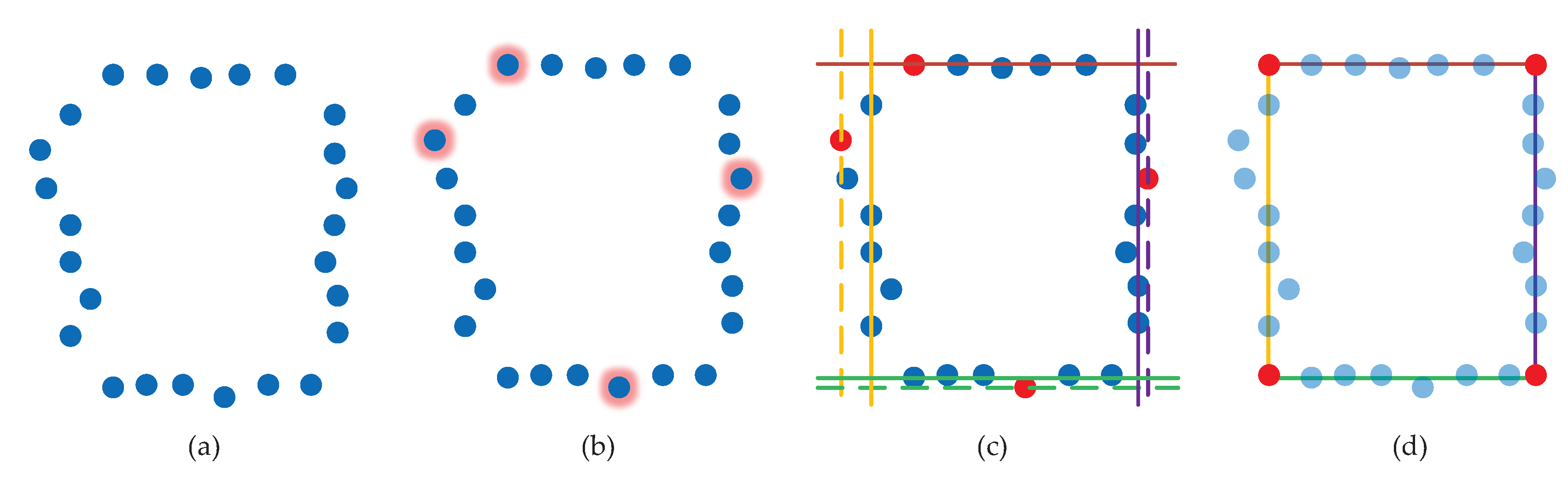
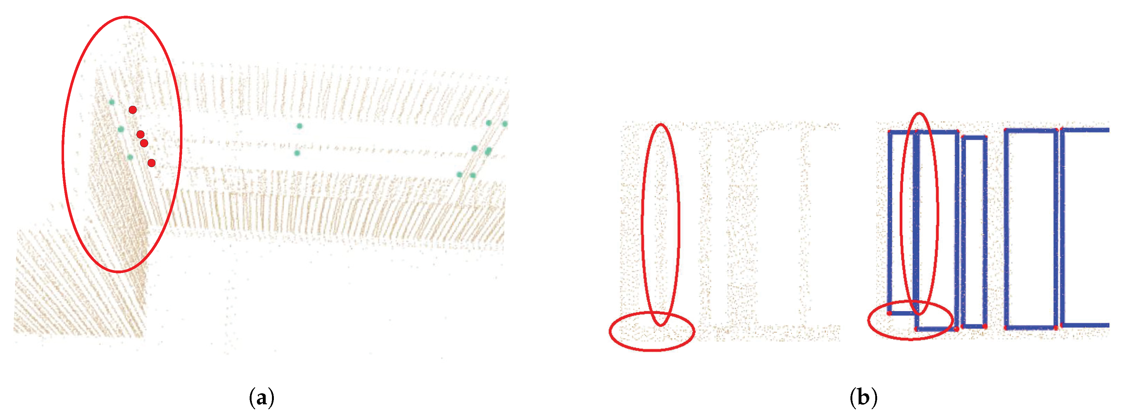
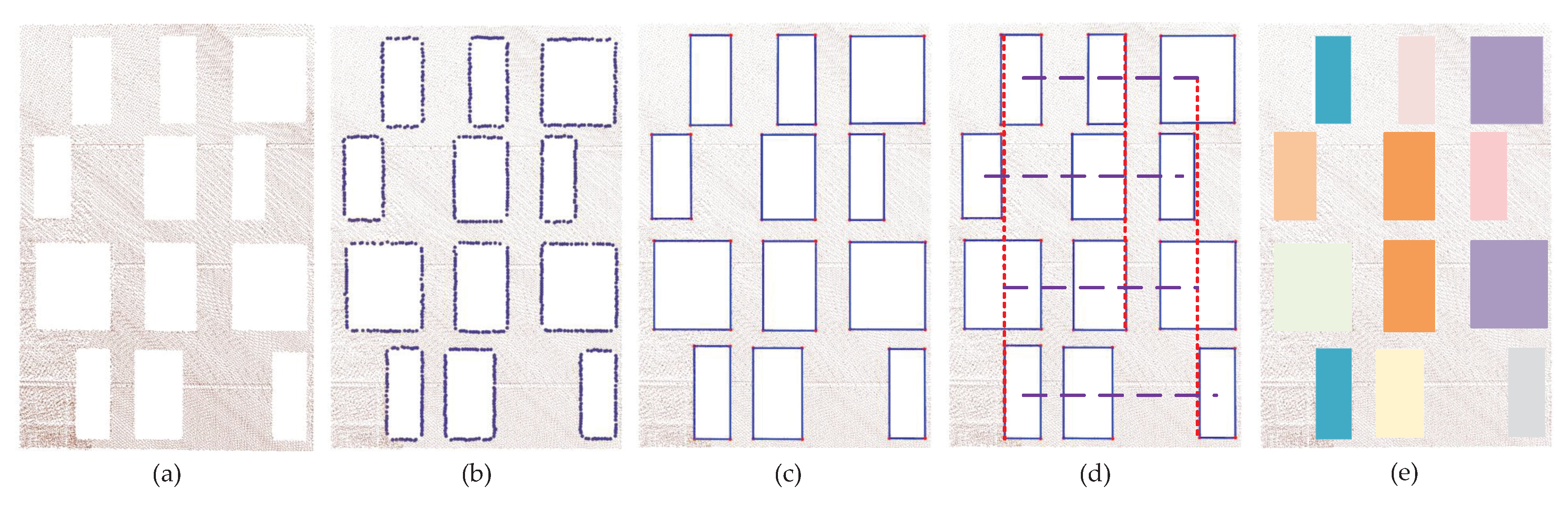
4.2. Boundary Extreme Point Detection
4.3. Opening Edge Fitting
4.4. Opening Reconstruction
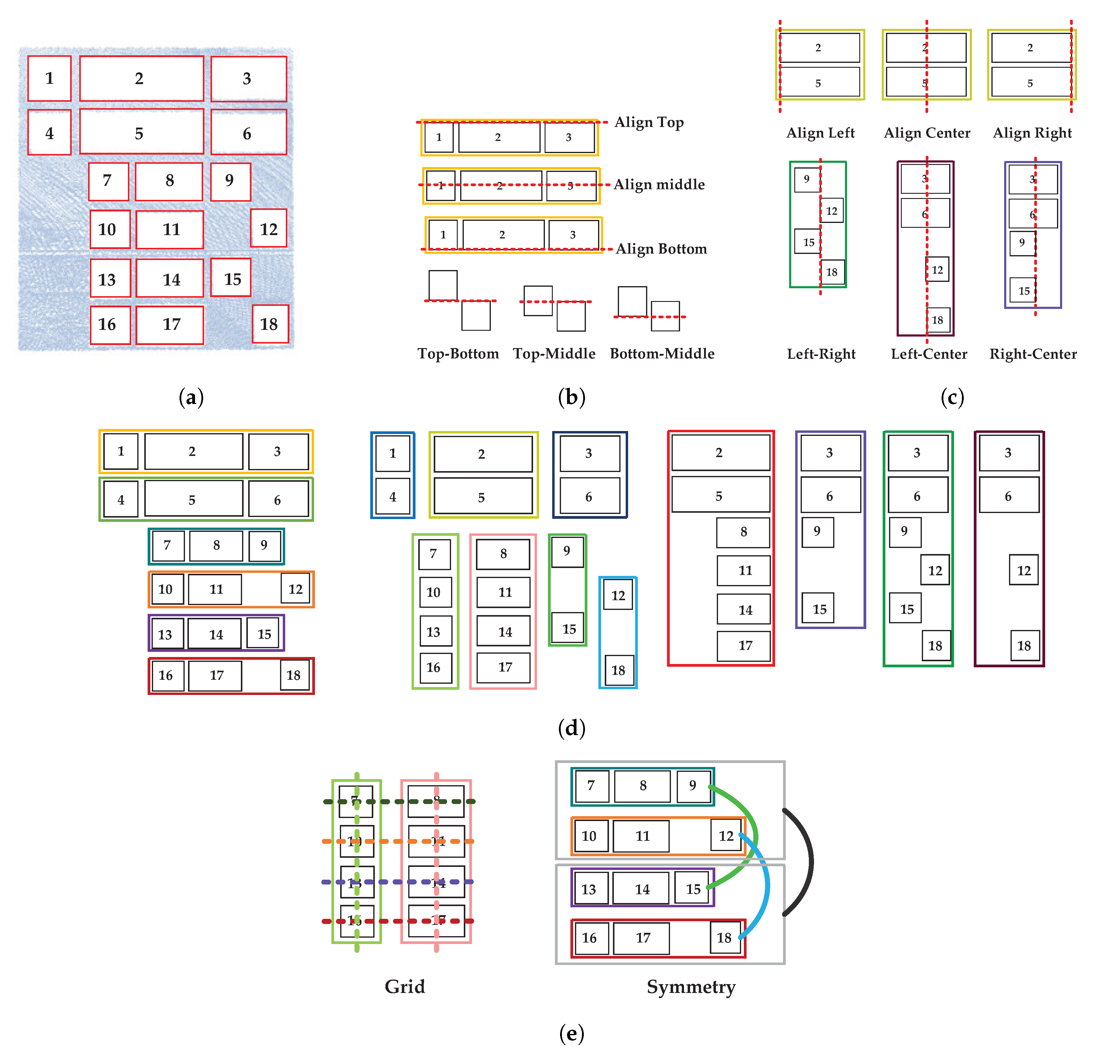
5. Global Alignment by Flexible Rules
| Algorithm 2: Opening Association and Alignment |
 |
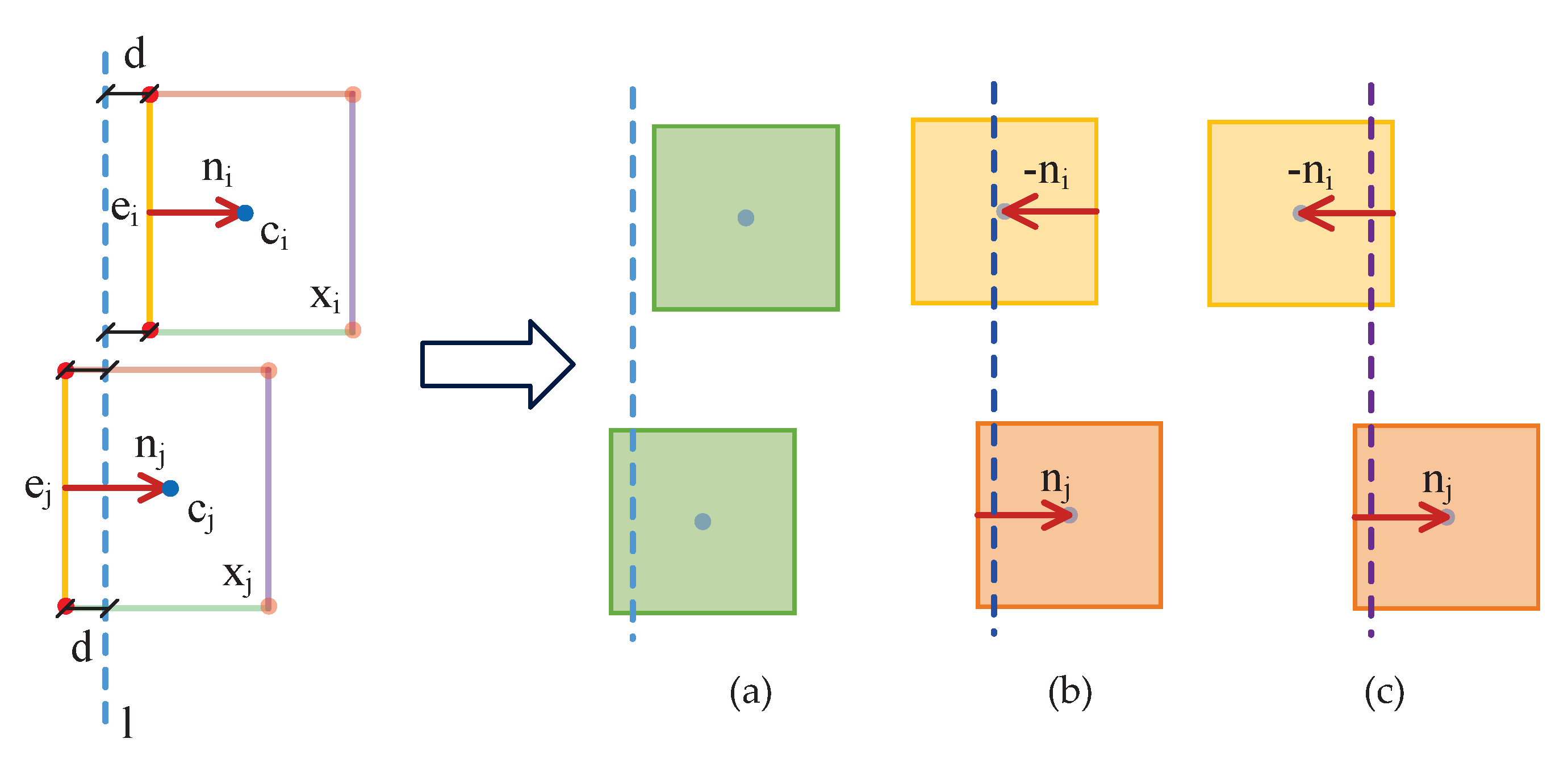
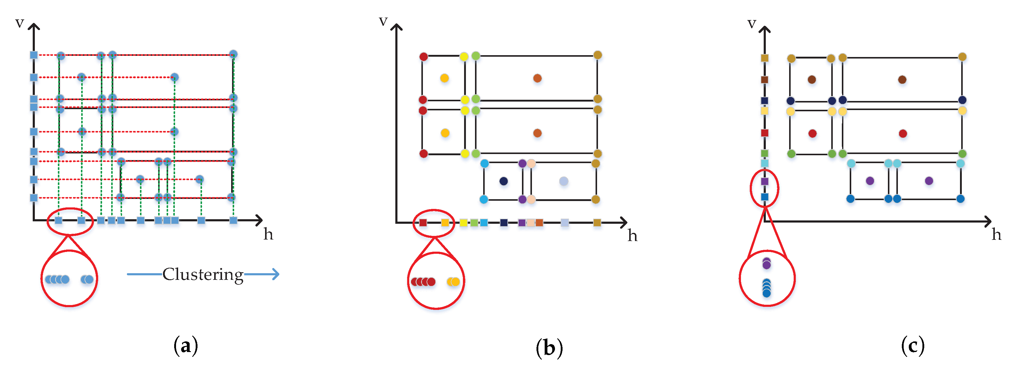
5.1. Flexible Rules
5.2. Opening Association Detection
5.3. Snapping
6. Experiments
6.1. Datasets
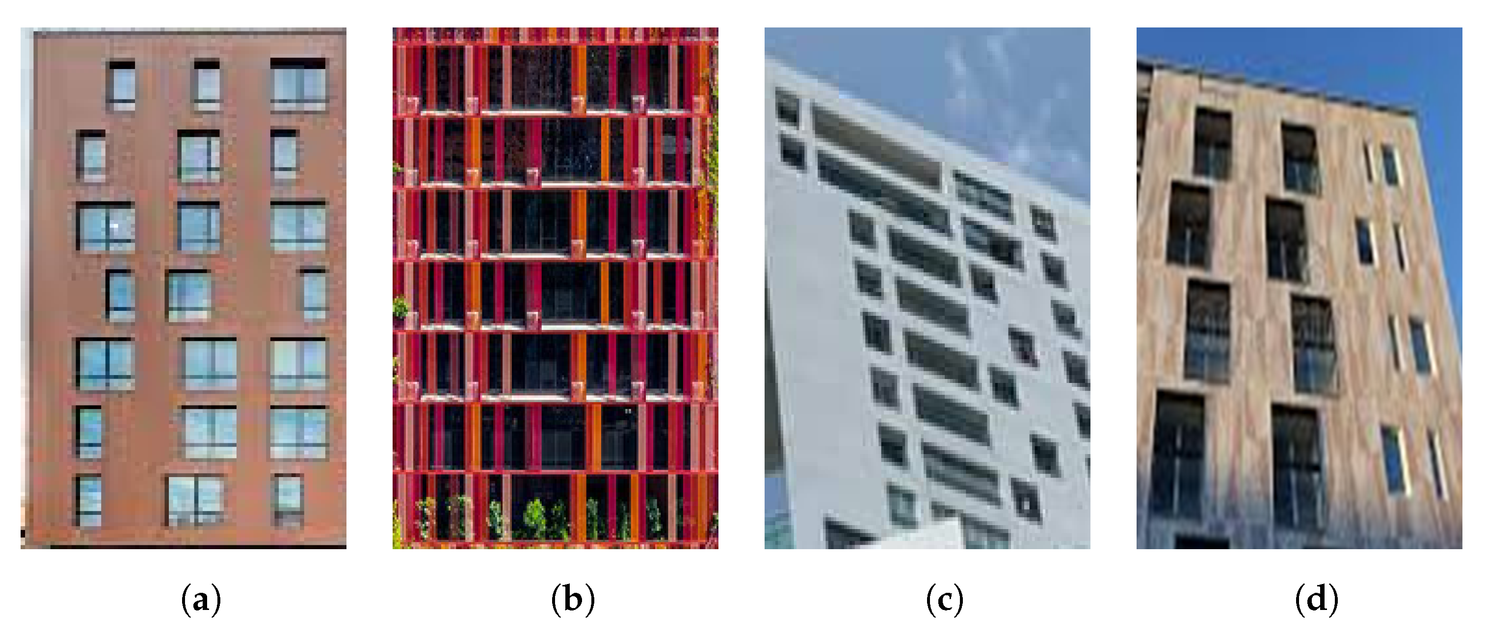
6.1.1. Outdoor Data
6.1.2. Indoor Data
6.2. Results
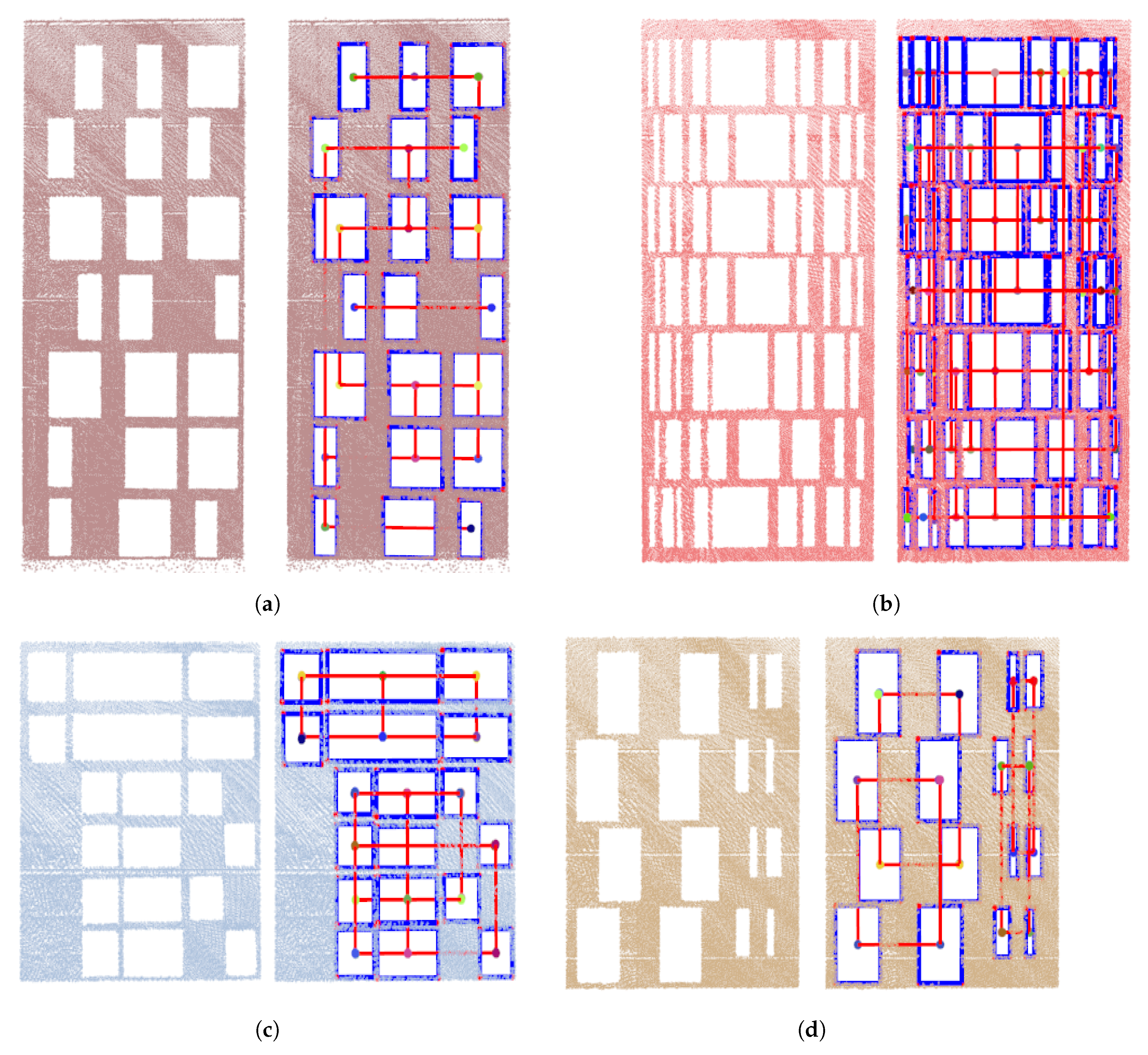
6.2.1. Outdoor Scenes
6.2.2. Indoor Scenes
6.2.3. Quantitative Evaluation
6.3. Discussions
6.3.1. Generality
6.3.2. Occlusions and Limitations
7. Conclusions and Future Work
Author Contributions
Funding
Acknowledgments
Conflicts of Interest
References
- Musialski, P.; Wonka, P.; Aliaga, D.G.; Wimmer, M.; van Gool, L.; Purgathofer, W. A Survey of Urban Reconstruction. Comput. Graph. Forum 2013, 32, 146–177. [Google Scholar] [CrossRef]
- Lafarge, F.; Mallet, C. Creating large-scale city models from 3D-point clouds: A robust approach with hybrid representation. Int. J. Comput. Vis. 2012, 99, 69–85. [Google Scholar] [CrossRef]
- Hepp, B.; Nießner, M.; Hilliges, O. Plan3D: Viewpoint and Trajectory Optimization for Aerial Multi-View Stereo Reconstruction. ACM Trans. Graph. 2018, 38, 4. [Google Scholar] [CrossRef]
- Nan, L.; Wonka, P. Polyfit: Polygonal surface reconstruction from point clouds. In Proceedings of the IEEE International Conference on Computer Vision, Venice, Italy, 22–29 October 2017. [Google Scholar]
- Poullis, C.; You, S. Automatic reconstruction of cities from remote sensor data. In Proceedings of the IEEE Conference on Computer Vision and Pattern Recognition, Miami, FL, USA, 20–25 June 2009. [Google Scholar]
- Gruen, A.; Schubiger, S.; Qin, R.; Schrotter, G.; Xiong, B.; Li, J.; Ling, X.; Xiao, C.; Yao, S.; Nuesch, F. Semantically Enriched High Resolution LOD 3 Building Model Generation. ISPRS Int. Arch. Photogramm. Remote Sens. Spat. Inf. Sci. 2019, XLII-4/W15, 11–18. [Google Scholar] [CrossRef] [Green Version]
- Gruen, A.; Schrotter, G.; Schubiger, S.; Qin, R.; Xiong, B.; Xiao, C.; Li, J.; Ling, X.; Yao, S. An Operable System for LoD3 Model Generation Using Multi-Source Data and User-Friendly Interactive Editing; Technical Report; Singapore ETH Centre, Future Cities Laboratory: Singapore, 2020. [Google Scholar] [CrossRef]
- Li, J.; Xiong, B.; Biljecki, F.; Schrotter, G. A sliding window method for detecting corners of openings from terrestrial LiDAr data. ISPRS Int. Arch. Photogramm. Remote Sens. Spat. Inf. Sci. 2018, XLII-4/W10, 97–103. [Google Scholar] [CrossRef] [Green Version]
- Rijal, H.; Tuohy, P.; Humphreys, M.; Nicol, J.; Samuel, A.; Clarke, J. Using results from field surveys to predict the effect of open windows on thermal comfort and energy use in buildings. Energy Build. 2007, 39, 823–836. [Google Scholar] [CrossRef] [Green Version]
- Cui, Y.; Li, Q.; Dong, Z. Structural 3D Reconstruction of Indoor Space for 5G Signal Simulation with Mobile Laser Scanning Point Clouds. Remote Sens. 2019, 11, 2262. [Google Scholar] [CrossRef] [Green Version]
- Mitra, N.J.; Guibas, L.J.; Pauly, M. Partial and approximate symmetry detection for 3D geometry. ACM Trans. Graph. 2006, 25, 560–568. [Google Scholar] [CrossRef]
- Müller, P.; Zeng, G.; Wonka, P.; Van Gool, L. Image-based procedural modeling of facades. ACM Trans. Graph. 2007. [Google Scholar] [CrossRef]
- Wang, R.; Bach, J.; Ferrie, F.P. Window detection from mobile LiDAR data. In Proceedings of the IEEE Workshop on Applications of Computer Vision, Kona, HI, USA, 5–7 January 2011; pp. 58–65. [Google Scholar]
- Wang, J.; Liu, C.; Shen, T.; Quan, L. Structure-driven facade parsing with irregular patterns. In Proceedings of the 3rd IAPR Asian Conference on Pattern Recognition, Kuala Lumpur, Malaysia, 3–6 November 2015; pp. 41–45. [Google Scholar]
- Whelan, T.; Goesele, M.; Lovegrove, S.J.; Straub, J.; Green, S.; Szeliski, R.; Butterfield, S.; Verma, S.; Newcombe, R.A.; Goesele, M.; et al. Reconstructing scenes with mirror and glass surfaces. ACM Trans. Graph. 2018, 37, 102. [Google Scholar] [CrossRef] [Green Version]
- Cohen, A.; Schönberger, J.L.; Speciale, P.; Sattler, T.; Frahm, J.M.; Pollefeys, M. Indoor-outdoor 3d reconstruction alignment. In Proceedings of the European Conference on Computer Vision, Amsterdam, The Netherlands, 11–14 October 2016; pp. 285–300. [Google Scholar]
- Huber, D.; Akinci, B.; Oliver, A.A.; Anil, E.; Okorn, B.E.; Xiong, X. Methods for automatically modeling and representing as-built building information models. In Proceedings of the NSF CMMI Research Innovation Conference, Atlanta, GA, USA, 4–7 January 2011. [Google Scholar]
- Xiong, X.; Adan, A.; Akinci, B.; Huber, D. Automatic creation of semantically rich 3D building models from laser scanner data. Automat. Constrn. 2013, 31, 325–337. [Google Scholar] [CrossRef] [Green Version]
- Becker, S.; Haala, N. Refinement of building fassades by integrated processing of lidar and image data. ISPRS Int. Arch. Photogramm. Remote Sens. Spat. Inf. Sci. 2007, 36, 7–12. [Google Scholar]
- Zolanvari, S.I.; Laefer, D.F. Slicing Method for curved façade and window extraction from point clouds. ISPRS J. Photogramm. Remote Sens. 2016, 119, 334–346. [Google Scholar] [CrossRef]
- Pu, S.; Vosselman, G. Knowledge based reconstruction of building models from terrestrial laser scanning data. ISPRS J. Photogramm. Remote Sens. 2009, 64, 575–584. [Google Scholar] [CrossRef]
- Edelsbrunner, H. Alpha shapes—A survey. Tessellations Sci. 2010, 27, 1–25. [Google Scholar]
- Edelsbrunner, H.; Kirkpatrick, D.; Seidel, R. On the shape of a set of points in the plane. IEEE Trans. Inform. Theory 1983, 29, 551–559. [Google Scholar] [CrossRef] [Green Version]
- Becker, S. Generation and application of rules for quality dependent façade reconstruction. ISPRS J. Photogramm. Remote Sens. 2009, 64, 640–653. [Google Scholar] [CrossRef]
- Wu, F.; Yan, D.M.; Dong, W.; Zhang, X.; Wonka, P. Inverse procedural modeling of facade layouts. ACM Trans. Graph. 2014, 33, 121. [Google Scholar] [CrossRef] [Green Version]
- Bao, F.; Schwarz, M.; Wonka, P. Procedural facade variations from a single layout. ACM Trans. Graph. 2013, 32, 8. [Google Scholar] [CrossRef] [Green Version]
- Pauly, M.; Mitra, N.J.; Wallner, J.; Pottmann, H.; Guibas, L.J. Discovering structural regularity in 3D geometry. ACM Trans. Graph. 2008, 27, 43. [Google Scholar] [CrossRef]
- Shen, C.H.; Huang, S.S.; Fu, H.; Hu, S.M. Adaptive partitioning of urban facades. ACM Trans. Graph. 2011, 30, 184. [Google Scholar] [CrossRef] [Green Version]
- Mesolongitis, A.; Stamos, I. Detection of windows in point clouds of urban scenes. In Proceedings of the IEEE Computer Society Conference on Computer Vision and Pattern Recognition Workshops, Providence, RI, USA, 16–21 June 2012; pp. 17–24. [Google Scholar]
- Nan, L.; Jiang, C.; Ghanem, B.; Wonka, P. Template assembly for detailed urban reconstruction. Comput. Graph. Forum. 2015, 34, 217–228. [Google Scholar] [CrossRef] [Green Version]
- Nan, L.; Sharf, A.; Zhang, H.; Cohen-Or, D.; Chen, B. Smartboxes for interactive urban reconstruction. ACM SIGGRAPH 2010, 29, 93. [Google Scholar] [CrossRef]
- Lafarge, F.; Descombes, X.; others. Geometric feature extraction by a multimarked point process. IEEE Trans. Pattern Anal. Mach. Intell. 2009, 32, 1597–1609. [Google Scholar] [CrossRef] [Green Version]
- Tournaire, O.; Brédif, M.; Boldo, D.; Durupt, M. An efficient stochastic approach for building footprint extraction from digital elevation models. ISPRS J. Photogramm. Remote Sens. 2010, 65, 317–327. [Google Scholar] [CrossRef] [Green Version]
- Tyleček, R.; Šára, R. A weak structure model for regular pattern recognition applied to facade images. In Proceedings of the Asian Conference on Computer Vision, Queenstown, New Zealand, 8–12 November 2010; pp. 450–463. [Google Scholar]
- Martinović, A.; Knopp, J.; Riemenschneider, H.; Van Gool, L. 3d all the way: Semantic segmentation of urban scenes from start to end in 3d. In Proceedings of the IEEE Conference on Computer Vision and Pattern Recognition, Boston, MA, USA, 7–12 June 2015; pp. 4456–4465. [Google Scholar]
- Vosselman, G. Automated planimetric quality control in high accuracy airborne laser scanning surveys. ISPRS J. Photogramm. Remote Sens. 2012, 74, 90–100. [Google Scholar] [CrossRef]
- Arikan, M.; Schwärzler, M.; Flöry, S.; Wimmer, M.; Maierhofer, S. O-snap: Optimization-based snapping for modeling architecture. ACM Trans. Graph. 2013, 32, 6. [Google Scholar] [CrossRef]
- Dechter, R.; Pearl, J. Generalized Best-First Search Strategies and the Optimality of A*. J. ACM 1985, 32, 505–536. [Google Scholar] [CrossRef]
- Rusu, R.B. Semantic 3d object maps for everyday manipulation in human living environments. Künstl. Intell. 2010, 24, 345–348. [Google Scholar] [CrossRef] [Green Version]
- Khoshelham, K.; Vilariño, L.D.; Peter, M.; Kang, Z.; Acharya, D. The ISPRS Benchmark on Indoor Modelling. ISPRS Int. Arch. Photogramm. Remote Sens. Spat. Inf. Sci. 2017, XLII-2/W7, 367–372. [Google Scholar] [CrossRef] [Green Version]
- Xu, Y.; Yao, W.; Tuttas, S.; Hoegner, L.; Stilla, U. Unsupervised segmentation of point clouds from buildings using hierarchical clustering based on gestalt principles. IEEE J. Sel. Top. Appl. Earth Obs. Remote Sens. 2018, 11, 4270–4286. [Google Scholar] [CrossRef]
- Vo, A.V.; Truong-Hong, L.; Laefer, D.F.; Bertolotto, M. Octree-based region growing for point cloud segmentation. ISPRS J. Photogramm. Remote Sens. 2015, 104, 88–100. [Google Scholar] [CrossRef]
- Rutzinger, M.; Rottensteiner, F.; Pfeifer, N. A comparison of evaluation techniques for building extraction from airborne laser scanning. IEEE J. Sel. Top. Appl. Earth Obs. Remote Sens. 2009, 2, 11–20. [Google Scholar] [CrossRef]


| Data | Type | Technique | Number of Points | Dimensions [m] | Clutter |
|---|---|---|---|---|---|
| Synthetic (a) | outdoor | MMS | 51,702 | Low | |
| Synthetic (b) | outdoor | MMS | 27,394 | Low | |
| Synthetic (c) | outdoor | MMS | 14,466 | Low | |
| Synthetic (d) | outdoor | MMS | 23,568 | Low | |
| KFH | outdoor | MMS | 161,470 | Moderate | |
| OKA | outdoor | TLS | 1,286,709 | High | |
| TUB1 | indoor | MMS | Low | ||
| TUB2 | indoor | MMS | Low | ||
| Fire Brigade | indoor | TLS | High | ||
| UVigo | indoor | MMS | Moderate | ||
| UoM | indoor | MMS | Moderate |
| Dataset | Syn. (a) | Syn. (b) | Syn. (c) | Syn. (d) | KFH | OKA | TUB1 | TUB2 | FB. | UVigo | UoM |
|---|---|---|---|---|---|---|---|---|---|---|---|
| Comp | 1 | 1 | 1 | 1 | 0.88 | 0.82 | 0.90 | 0.85 | 0.86 | 0.68 | 0.73 |
| Corr | 1 | 0.94 | 1 | 1 | 0.93 | 0.96 | 0.93 | 0.91 | 0.91 | 0.86 | 0.67 |
| F1 | 1 | 0.97 | 1 | 1 | 0.90 | 0.89 | 0.92 | 0.88 | 0.89 | 0.76 | 0.70 |
| Dataset | Syn. (a) | Syn. (b) | Syn. (c) | Syn. (d) | KFH | OKA | TUB1 | TUB2 | FB. | UVigo | UoM |
|---|---|---|---|---|---|---|---|---|---|---|---|
| MPS | 0.030 | 0.030 | 0.030 | 0.030 | 0.030 | 0.011 | 0.005 | 0.008 | 0.011 | 0.010 | 0.007 |
| NoO | 21 | 62 | 18 | 12 | 16 | 204 | 30 | 72 | 253 | 30 | 15 |
| D (bef.) | 0.057 | 0.099 | 0.075 | 0.056 | 0.062 | 0.119 | 0.023 | 0.026 | 0.127 | 0.038 | 0.035 |
| D (aft.) | 0.053 | 0.088 | 0.060 | 0.051 | 0.044 | 0.117 | 0.023 | 0.021 | 0.124 | 0.033 | 0.030 |
| rate | 7% | 11% | 20% | 9% | 29% | 2% | 0% | 19% | 2% | 13% | 14% |
© 2020 by the authors. Licensee MDPI, Basel, Switzerland. This article is an open access article distributed under the terms and conditions of the Creative Commons Attribution (CC BY) license (http://creativecommons.org/licenses/by/4.0/).
Share and Cite
Li, J.; Xiong, B.; Qin, R.; Gruen, A. A Flexible Inference Machine for Global Alignment of Wall Openings. Remote Sens. 2020, 12, 1968. https://doi.org/10.3390/rs12121968
Li J, Xiong B, Qin R, Gruen A. A Flexible Inference Machine for Global Alignment of Wall Openings. Remote Sensing. 2020; 12(12):1968. https://doi.org/10.3390/rs12121968
Chicago/Turabian StyleLi, Jiaqiang, Biao Xiong, Rongjun Qin, and Armin Gruen. 2020. "A Flexible Inference Machine for Global Alignment of Wall Openings" Remote Sensing 12, no. 12: 1968. https://doi.org/10.3390/rs12121968
APA StyleLi, J., Xiong, B., Qin, R., & Gruen, A. (2020). A Flexible Inference Machine for Global Alignment of Wall Openings. Remote Sensing, 12(12), 1968. https://doi.org/10.3390/rs12121968