1. Introduction
Current global developments are putting increasing ecological, economic, and social pressure on urban systems [
1]. In Africa, where 64% of the population will be urban by 2050 [
2], controversies about urban agriculture’s contribution to city’s resilience are growing [
3,
4]. Many authors underline urban agriculture’s positive role in city food supply, employment, or protection against flooding [
5], while others consider agriculture as a source of nuisance for the city through livestock effluents or the poor sanitary quality products it generates [
6]. Hence, both researchers and planners underline the need to better characterize and monitor city–agriculture interactions to help develop appropriate policies [
7].
Urban systems are among the most complex ecosystems because they are characterized by a large number of diverse components, nonlinear interactions, and spatial heterogeneity [
8]. Remote sensing data have been widely used to characterize and monitor urban systems (with several limitations) [
9], focusing mostly on urban components (buildings, house, roads, and so on) [
10,
11] and less often on agricultural components (urban agricultural plots, urban orchards, and so on) [
12,
13]. However, little effort has been devoted to simultaneously mapping urban and agricultural spaces in southern cities and their dynamics [
14]. The challenges are indeed numerous. On one hand, urban agriculture is characterized by high heterogeneity, uncertain boundaries, small fields, and high fragmentation owing to multiple adjacent land uses [
13]. On the other hand, urban elements are characterized by spatial and spectral heterogeneity [
15,
16,
17], are very small in size, and may be made of natural materials (thatched roof, mud bricks), making it difficult to differentiate them from non-urban uses (bare soils, agricultural residues, and so on).
Standard remote sensing techniques are not appropriate to map smallholder cropping systems in urban areas, where fields and built-up objects are often smaller than the spatial resolution of readily available low spatial resolution (LSR) data, such as MODIS (Moderate Resolution Imaging Spectroradiometer, 250 m resolution) and even medium spatial resolution (MSR) Landsat data (30 m resolution) [
18]. New opportunities for the mapping of urban and agriculture land in cities are now available thanks to recent satellite missions, offering high spatial (HSR) and temporal resolution time series such as Sentinel 2 (10 m/5 days), or very high spatial resolution (VHSR) images (<5 m) such as Pleiades. The combination of these multi-source data appears to be an interesting way to identify urban agricultural plots [
13]. On one hand, very high spatial resolution images enable the detection of small objects such as fields surrounded by built-up objects. On the other hand, time series of decametric images are useful to characterize smallholder agriculture as they record the phenological changes in crop reflectance linked with seasonal cycles at a suitable spatial resolution. Data derived from time series and very high spatial resolution images represent a large volume of data that remains a significant challenge for the automated mapping of agricultural land and urban objects [
19]. Emerging machine learning techniques are currently receiving increasing attention in the literature [
20,
21]. Among them, the random forest ensemble method is increasingly frequently used for land cover classification from multi- or hyper-spectral imagery [
18,
20,
22]. Such techniques can be combined with object based image analysis (OBIA), which has proven to be an effective way to analyze very high spatial resolution images, especially in urban areas [
23], as well as to map smallholder agriculture [
18]. OBIA minimizes confusion during classification by incorporating information that takes human pattern recognition into account. Before the classification step, pixels are first grouped into objects based on either spectral or thematic similarity using a segmentation algorithm. In addition to spectral information, texture features can also be calculated to obtain information on the spatial arrangement of the pixels.
This paper has three main objectives. The first is to describe the methodology we used to simultaneously map urban and agricultural spaces in a southern city. The second one is to use remote sensing data to better understand agri-urban landscapes and city-agriculture interactions. The third objective is to quantify agricultural functions: how many urban households are involved in agricultural activities? How much food does urban agriculture supply? Is there competition between urban expansion and agriculture? In a context where geographical and statistical institutions struggle to produce data, all these results provide valuable information for decision makers.
To achieve these objectives, the approach first produced a land cover map at three (nested) nomenclature levels showing agricultural areas and urban spaces. It combines the use of VHSR Pleiades imagery and HSR satellite image time series (Sentinel 2 and Landsat 8) in an OBIA and random forest approach. The approach then produced a second map, based on the analysis of the spatial patterns of land use classes, to define an “agri-urban landscape”. It finally enabled the identification and quantification of agricultural functions within the city. The approach mixes the analysis of land use and agri-urban landscape maps combined with ancillary data (demographic and agricultural census, among others).
We tested this approach in Greater Antananarivo. The capital of Madagascar is an archetype of an urban setting where built-up areas are closely interwoven with agricultural land. As a source of food, employment, and resilience for the city against floods, agriculture is a major pillar of city resilience [
24].
This approach has major implications for public actions. Policy debates are underway to update urban development and sanitation master plans. So far, however, stakeholders have neither reliable land-use maps of the city nor recent data on urban agriculture (surface area, number of producers, quantity of food produced). This analysis is thus of prime importance to feed the debate on urbanization, the functions of urban agriculture, and the best way to enhance the resilience of Antananarivo city.
In the rest of this paper, we successively describe (i) the procedures used to develop the land-use map, its characteristics, and its reliability; (ii) the procedure used to develop the agri-urban landscape map and its composition /pattern; and (iii) the analysis of urban agriculture main functions in terms of food security, employment, and interactions with the city.
2. Materials and Methods
2.1. Study Area
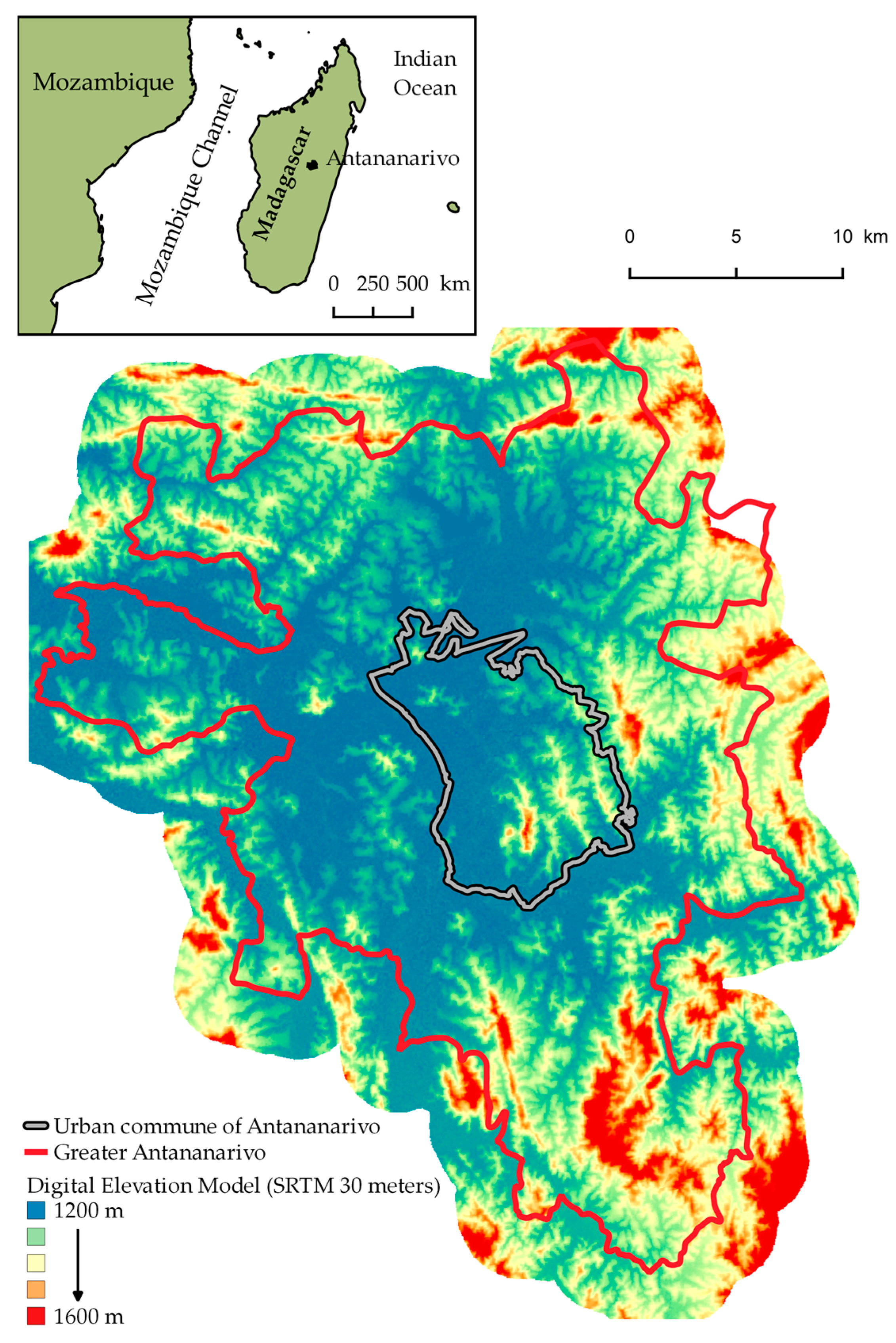
Madagascar is an island country located in the Indian Ocean off the coast of Mozambique. The study zone (
Figure 1) includes the entire area (770 km²) of Greater Antananarivo, the capital and at the same time the largest city in Madagascar. Antananarivo is located in the center of the island at 1280 m above sea level. The topography is characterized by a large floodplain in the western part of the city, bordered by a succession of hills in the eastern part. Greater Antananarivo is made up of 38 municipalities, including the Urban Commune of Antananarivo (UCA), in the center, which houses the historic heart of the city. In terms of demography, Great Antananarivo has a high population density compared with other Malagasy cities, with 780 inhabitants per km² on average, and 18,000 inhabitants per km² in the UCA (which is comparable to the most densely populated cities in the world). In 2015, the estimated total population was three million inhabitants [
25].
Greater Antananarivo is characterized by dense built-up areas in the center connected to peripheral urban nodes. The presence of the agricultural floodplain in the western part of the city has curbed the progress of the built-up areas, favored its expansion in the eastern part, and encouraged the densification of older urban nodes in the periphery. The buildings are heterogeneous, with a mixture of residential houses made of brick or concrete, on average >60 m² in size, and precarious houses made of wood with a straw roof, on average <15 m² in size. The land use of a large part of Greater Antananarivo is agricultural, comprising small family farms that rely on manual labor, with a high diversity of crops, small fields (<0.05 ha), and crop rotations in space and time.
2.2. Earth Observation Data Acquisition and Preprocessing
Figure 2 shows the chronogram of the satellite images acquired between October 2016 and September 2017. Different types of satellite data were used:
High spatial resolution (HSR) data, corresponding to a time series of 19 images from Landsat-8 OLI (Operational Land Imager)/TIRS (Thermal InfraRed Sensor) and 62 images from Sentinel-2 (2 tiles and 31 acquisition dates);
VHSR resolution data, with two 20 × 20 km Pleiades tiles acquired simultaneously on 8 January 2017, which corresponds to the middle of the rainy season. However, owing to a delay in the start of the rainy season, all the crops are not visible in the image.
Additionally, the shuttle radar topography mission (SRTM) digital elevation model (DEM) at 30 m spatial resolution was downloaded from the United States Geological Survey (USGS) website to account for the topography (altitude, slope) of the study area, which can help distinguish some land use classes (e.g., irrigated crops in the lowlands vs. rainfed crops in the hills).
Finally, the “Orthobase Madagascar” product, an orthorectified mosaic of 2.5 m panchromatic SPOT5 images distributed by SEAS-OI (Survey of the Environment Assisted by Satellite in the Indian Ocean) receiving station was acquired to serve as a reference for the co-registration of Pleiades images.
The two Pleiades tiles were delivered by AIRBUS Defense and Space at primary level (without radiometric or geometric corrections). Preprocessing steps were carried out with Orfeo ToolBox (OTB available at
https://www.orfeo-toolbox.org) [
26] and consisted of top of atmosphere (TOA) reflectance calculation, and orthorectification of panchromatic (PAN, 0.5 m spatial resolution) and multispectral (MS, 2 m spatial resolution) images using SRTM DEM and ”Orthobase Madagascar”, a homologous point extraction process. The two PAN and MS tiles were then mosaicked and the resulted mosaics were pansharpened using the Bayesian fusion algorithm of the OTB pansharpening module [
27] to obtain a multispectral mosaic at 0.5 m spatial resolution.
Sentinel-2 (European Spatial Agency (ESA)) and Landsat-8 (National Aeronautics and Space Administration (NASA)) images were downloaded from Amazon Web Service (AWS). Landsat-8 PAN (15 m spatial resolution) and MS (30 m spatial resolution) images (except 30 m bands 1 and 9 corresponding to coastal/aerosol and cirrus bands, respectively, and 100 m 10 and 11 thermal infrared bands) were pansharpened using the Bayesian fusion algorithm to obtain multispectral images at 15 m spatial resolution.
Two Sentinel-2 tiles were necessary to cover the whole study area. The 62 tiles were mosaicked to produce a time series of 31 mosaics. Spectral bands with 60 m spatial resolution of little interest for the classification (B1—aerosols, B9—water vapor, and B10—cirrus) were discarded; 20 m spatial resolution bands (redegde and near infrared bands: B5, B6, B7, B8a, as well as short wave infrared bands: B11 and B12) were resampled at 10 m resolution. Although already orthorectified, Sentinel-2 and Landsat-8 images were readjusted on the VHSR Pleiades coverage using the homologous point extraction process of OTB. Finally, the Fmask tool [
28] was used to produce the cloud masks corresponding to each image of the time series and a gap filling linear interpolation was applied using OTB Temporal Gap Filling remote module (available at
http://tully.ups-tlse.fr/jordi/temporalgapfilling) to interpolate the cloudy pixels in the time series.
2.3. Field Measurements and Nomenclature
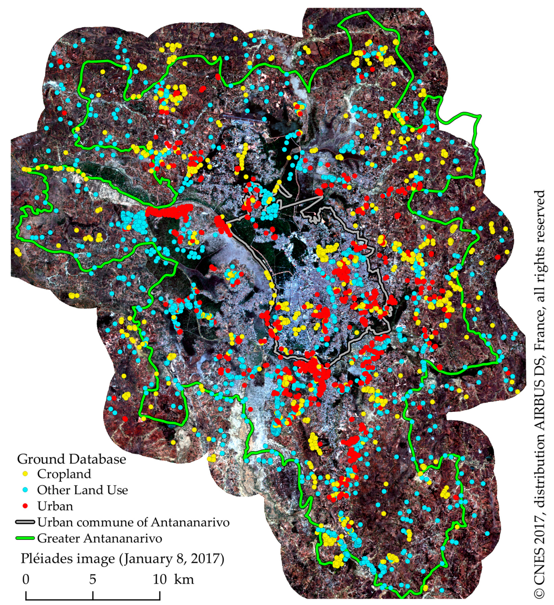
Field surveys were performed during the end of the 2017 rainy season (March to April), which corresponds to the peak growing season. GPS (Global Positioning System) waypoints were collected using an opportunistic sampling approach [
18]. Waypoints were collected throughout the study area to be representative of existing types of crops and urban structures. GPS points were also recorded for uncultivated and unbuilt classes such as natural spaces or water bodies. Each waypoint was then converted into a polygon by digitizing the boundaries of the corresponding land cover on a VHSR Pleiades image (0.5 m × 0.5 m pixel size). A total of 981 additional polygons were digitized by photointerpretation of the Pleiades image for easily recognizable classes (housing, brick extraction, rice, watercress, and savannah). The final ground database was thus composed of 3068 polygons including 1373 cropped, 813 urban, and 882 other land uses.
Figure 3 shows their locations.
Agricultural plots were recorded using the nomenclature listed in
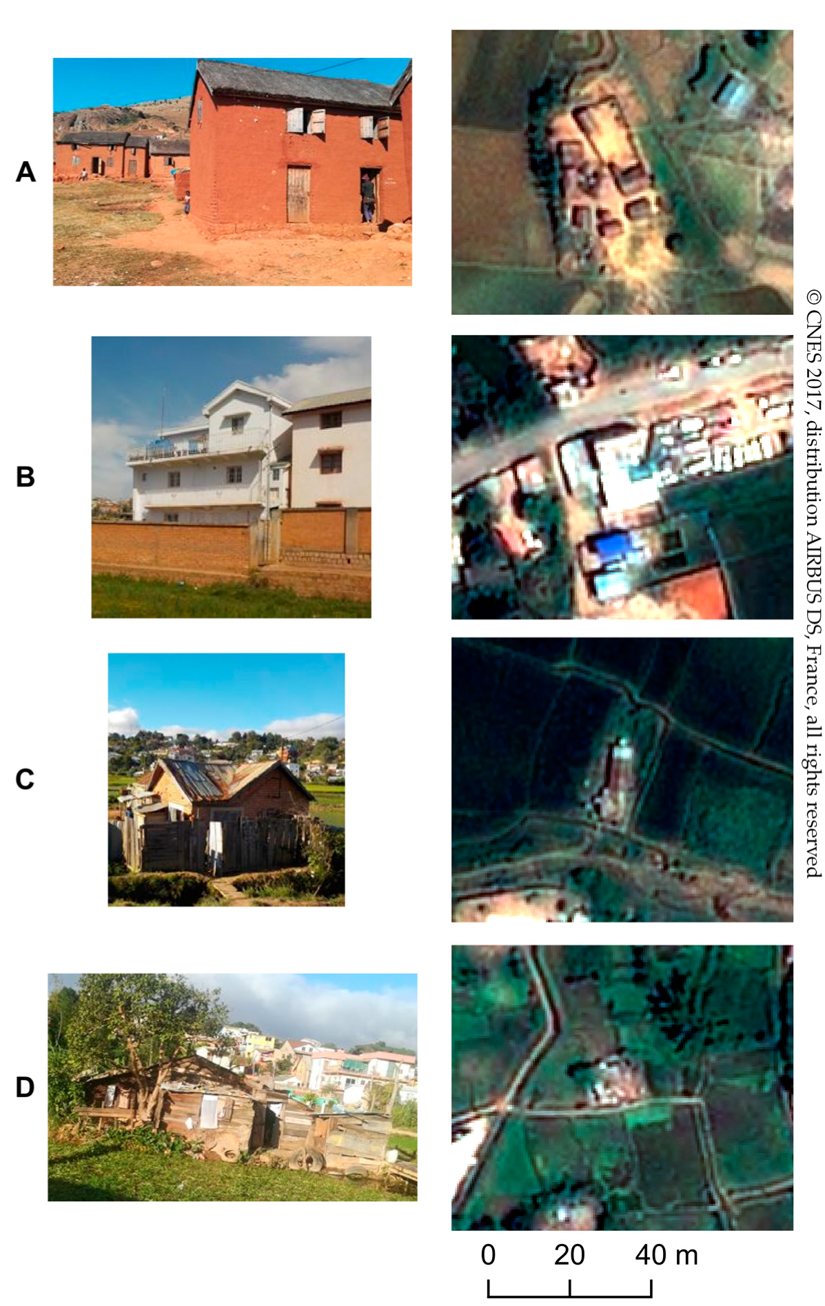
Table 1. Additional information on cropping practices, irrigation systems, mixed cropping, and so on was also recorded at each GPS point. For urban objects, the nomenclature was based on field observations and six classes were defined: (1) mixed habitat, (2) residential area, (3) rural housing, (4) industrial, commercial and military area, (5) brick extraction sites, and (6) quarry landfill and construction site. The field photographs and corresponding satellite images in
Figure 4 illustrate (i) the variability between and within urban classes and (ii) the small size of urban objects compared to agricultural fields (pictures A to D). This high variability is represented using a nomenclature based on three levels of detail ranging from the most general (level 1—cropland: 2 classes) to the most precise (level 3—crop class: 20 classes) (see
Table 1).
2.4. Methods
The land cover map at the three nomenclature levels was produced using the Moringa processing chain, recently presented at the ESA Living Planet Symposium [
29] and already used to produce a publicly available VHSR land cover map of Reunion Island, [
30]. Its classification strategy builds on the one described in [
18] and involves three main steps: (i) segmentation of the VHSR Pleiades mosaic to produce homogeneous objects; (ii) object level extraction of spectral and textural features from satellite images and other products (DEM); and (iii) the training and validation of a random forest classifier for each level of the nomenclature, which was then applied to the whole study area to produce the land use maps. All three steps were performed using OTB functions driven by Python scripts.
Agri-urban landscape zoning of the agglomeration was derived from the resulting land cover maps to help understand the interactions between agricultural and urban spaces. The main agricultural functions were then derived through an analysis of land cover and zoning maps, coupled with field studies.
2.4.1. Land Cover Classification
We used a method based on three main steps:
In this study, the large scale generic region merging (LSGRM) remote module for OTB (adapted from [
31] and available at
https://gitlab.irstea.fr/remi.cresson/LSGRM) was used for the segmentation step, which was applied to the four spectral bands of the Pleiades pansharpened mosaic. After various setup tests over different subsets of the study area, the following segmentation parameters were empirically selected to clearly detect the boundaries of fields and urban objects: scale parameter—150; weight parameter on the shape—0.3, and weight parameter on compactness—0.7.
Various features were extracted from the satellite data: (i) reflectances and (ii) spectral indices from the HSR times series, (iii) textural indices from the VHSR Pleiades panchromatic mosaic, and (iv) altitude and slope from SRTM DEM. For all these features, the average value per object of the segmentation was extracted.
Concerning the reflectances, average values were extracted for eight bands of Landsat-8 images and 10 bands of Sentinel-2 images (see
Table 2). As explained previously, specific bands such as aerosols, thermal infrared, or water vapor and cirrus bands were eliminated from the images of these two sensors.
The spectral indices were selected based on their ability to distinguish between the different classes of the nomenclature. The normalized difference vegetation index (NDVI [
32]) and modified normalized difference vegetation index (MNDVI [
33]) were used to characterize crop type, as well as the rededge NDVI (RNDVI [
34]), which exploits the spectral richness of Sentinel-2 data. Given the presence of irrigated rice, the normalized difference water index (NDWI [
35]) and the modified normalized difference water index (MNDWI [
36]) were also selected for their sensitivity to the presence of water. Finally, the brightness index (Euclidean norm of the surface reflectances) was also calculated.
Textures calculated from the VHSR Pleiades images were used to help distinguish some classes that had specific very small patterns that cannot be detected in the HSR time series such as urban areas and orchards. The textures were calculated from the panchromatic band of the Pleiades mosaic using the Haralick texture extraction tool of OTB. Different textures (four indices) and window sizes (seven window sizes) were tested over several representative subsets of the study area. Finally, three indices (contrast, energy, and variance) and two window sizes (5 × 5 and 11 × 11 pixels) were selected visually for their ability to distinguish, for example, orchards (with high contrast or variance and low energy) from rice (high energy), or to help identify urban areas (very high contrast and variance values).
Finally, mean altitude and slope were extracted from the SRTM DEM.
Table 2 lists the 732 features obtained. Features extracted from the HSR time series predominated with 724 features.
For the classification step, the random forest ensemble method was chosen for its ability to handle a large volume of features; its stability; robustness; ease of use (few user-defined parameters); and accuracy, which has been shown to be the same as—or better than—other algorithms such as decision trees [
37] and support vector machines [
38]. Random forest builds forests of classification trees from random sample sets produced using a bagging-based approach. An out-of-bag (OOB) error can be calculated from one-third of the data randomly excluded from the construction of each classification tree. An OBB corresponds to the rate of misclassified samples. Calculating this internal error makes it possible to use the entire ground sample database to train the random forest (RF). However, the OOB error was shown to be overestimated in balanced settings and in settings with few observations and with a large number of predictor variables. The authors of [
39] thus recommend using stratified subsampling for error estimation in RF, and the authors of [
40] recommend adding a cross-validation process to reduce the remaining bias.
After having divided the ground database into five roughly equal subsets, a fivefold cross validation was performed by training RF five times with four subsets and validating with the remaining one so that each subset was used once for validation. The final accuracy was obtained by averaging the overall accuracies (corresponding to the total surface of correctly classified objects divided by the total surface of test objects) and Cohen’s kappa (which reflects the difference between actual agreement and agreement expected by chance) in all five cases of cross validation. For a specific class, accuracy was summarized using the F1-score, which was calculated as the harmonic mean of producer and user accuracies. This procedure was used for each level of the nomenclature.
The classifiers obtained for each level were then used to predict the classes of all the objects in the study area and to produce three maps (one for each nomenclature level).
2.4.2. Agri-Urban Landscape Zoning
The organization of agricultural and urban landscapes within the city was analyzed according to the presence and spatial arrangement of various agricultural and urban land use classes within the territory. To this end, a 2 × 2 km grid was generated, and each cell of the grid was classified using a k-mean (with k = 4) clustering of seven variables: (i) the proportion of five classes “Natural_Spaces”, “Built_up_surfaces”, “Watercress”, “Rice”, and “Other_Crops”, (ii) the aggregation index [
41], referred to as AI, calculated using Fragstats [
42] for the class “cropland” of the first level of the nomenclature, and for the class “urban area” of the second level of the nomenclature. These two last features were chosen to reflect whether cropland and urban patches are aggregated (AI = 100) or not (AI = 0) over Greater Antananarivo.
2.4.3. Urban Agriculture Functions and Competition Between Urban Expansion and Agriculture
Two main functions of urban agriculture were estimated based on the resulting land cover maps and a literature review: (i) employment and (ii) city’s food supply.
Estimation of the number of urban households involved in agricultural activities was based on total surface area of cropland and average farm area per household in Greater Antananarivo according to the literature and field studies.
The contribution of urban agriculture to the city’s food system was calculated using the surface area of cropland for specific classes (rice and watercress) and associated average yields according to data in the literature.
Competition between agricultural and urban land uses is discussed based on the analysis of the land use maps and agri-urban landscape zoning.
3. Results
3.1. Analysis of Land Use Classification Scores
At level 1, crop and non-crop classes were distinguished with an overall accuracy of 94.78% and a Cohen’s kappa of 0.88 (see
Table 3).
As shown in
Table 3, overall accuracy at level 2 was 86.83%, but decreased to 76.56% at level 3. The same trend was observed for Cohen’s kappa.
Table 4 lists classification F1-scores for crop and non-crop classes at the different nomenclature levels. It highlights the good classification results for urban spaces (91.63%) and annual and pluriannual crops at level 2 (91.6% and 88.5%, respectively). At level 3, only a few classes were well classified including rice fields (the main crop grown on agricultural land), watercress, and brick extraction sites (88.0%, 78.3%, and 94.7%, respectively).
The analysis of the classification results shows that some classes are particularly difficult to identify. A detailed analysis of the confusion matrix obtained at level 3 (not shown here) and the observation of Peiades image allowed us to identify the main cases of confusion responsible for the low scores. Two examples are given below for “Cassava”, a crop class, and for “rural housing”, an urban class.
Considering the “cassava” class (F1-score of 48.6%), the poor user accuracy (49%) was linked to the fact that many objects classified as cassava were in fact “Bare non-agricultural soil”; “Vegetable crop”; “Fallows, pasture, and bare agricultural soil”; or “Herbaceous savannah”. Poor producer precision (44%) was linked to the fact that many objects that should have been classified as cassava were classified in other crop classes or as natural spaces. The similarity between cassava fields and their direct environment is the source of these cases of confusion. Cassava is grown in very small fields on the uplands (called tanety). The cropping cycle is two years, with marked morphological differences in the first and the second year.
Considering the “rural housing” class (F1-score of 52.77%), user accuracy was low (49%) meaning that an average of 51% of objects were classified as rural housing, whereas they were in fact actually “Mixed habitat”, “Quarry”, “Fruit crop” or "Vegetable crop”, and “Herbaceous savanna” classes. Producer precision was also poor (36%), with many objects that should have been classified as traditional habitat actually classified as “Mixed habitat”. These cases of confusion with other urban classes, as well as with crop classes, illustrate the difficulty of differentiate rural housing when it is constructed using natural materials taken from the immediate vicinity of the housing such as mud, thatch, or stones.
3.2. Land Use Maps at Four Different Nomenclature Levels
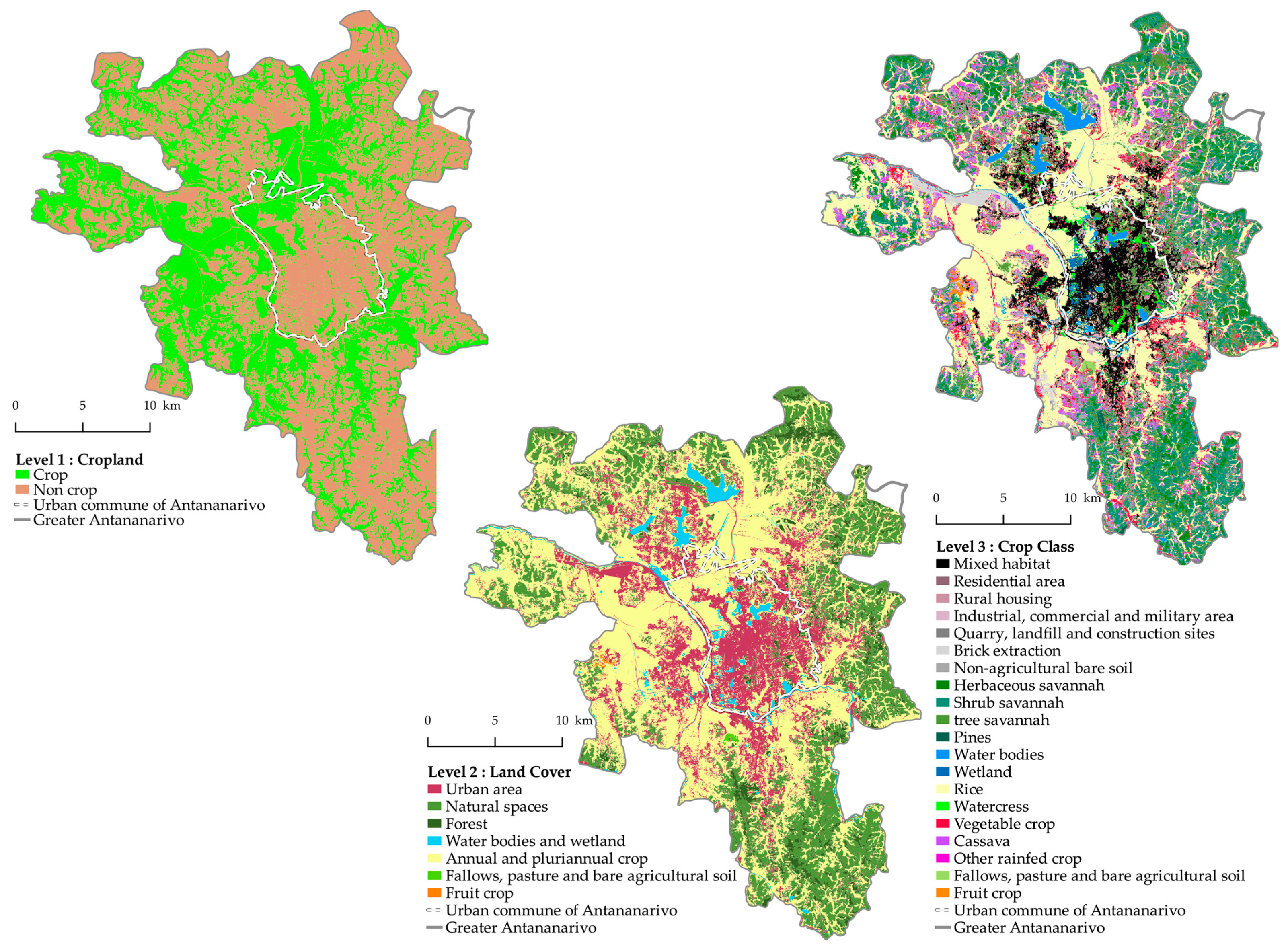
Figure 5 presents the land use maps of Greater Antananarivo obtained at levels 1 to 3.
The level 1 classification results show that almost half (44%) of Greater Antananarivo and more than one-third (35%) of the city center is cultivated. Within the cultivated area, rice fields dominate, followed by watercress in the city center. The agricultural landscape is thus mainly composed of irrigated crops, which account for more than two-thirds (70%) of cultivated land in Greater Antananarivo. At level 3, the other major crops are vegetable crops, followed by cassava and tree crops (15%, 12%, and 2% of the total cultivated area, respectively).
Urban spaces account for almost one-fifth (18%) of Greater Antananarivo and almost half (49%) of the city center. Within these urban spaces, individual houses dominate (80%), followed by brick quarries (14%), a land use undergoing marked expansion as the quarries supply the city with construction materials. In the city center, individual houses clearly dominate (close to 90% of the urban area), followed by the industrial and commercial zones that characterize the city landscape locally (6% of the total urban area).
At the scale of Greater Antananarivo, natural areas (savannah, forest, and so on) account for a larger area (37%) than urban spaces. In contrast, in the city center, natural areas only account for 8%, and are mainly composed of urban green spaces, water bodies, and wetlands. Note that all these proportions should be interpreted in light of the corresponding classification accuracies.
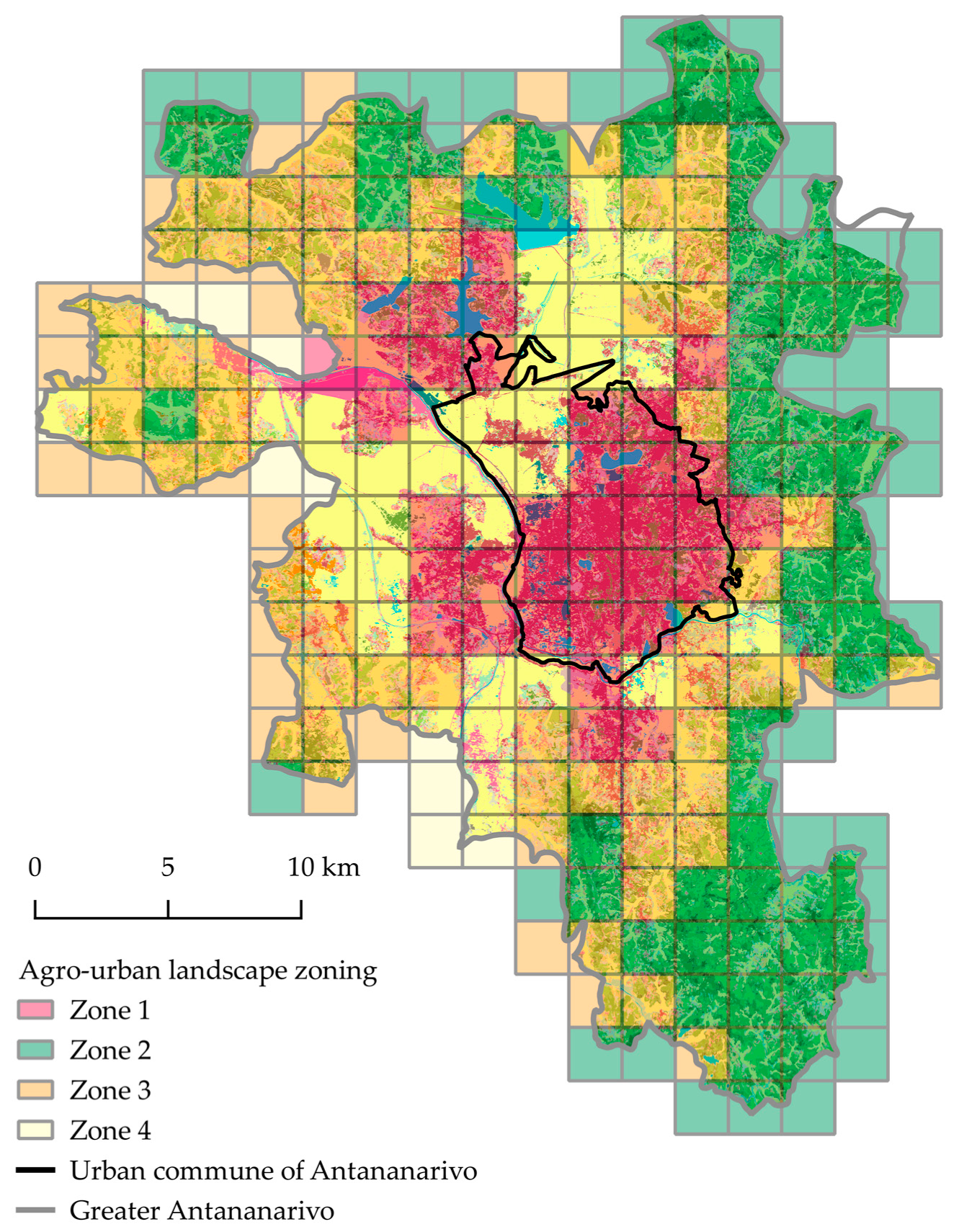
3.3. Agri-Urban Landscapes Zoning Analysis
Figure 6 shows the agri-urban zoning of Antananarivo associated with the average values of the seven variables used for the k-means clustering (
Table 5). The four zones have specific characteristics in terms of class composition and organization. In the core urban area (Zone 1), in the center of the agglomeration, the landscape is characterized by extremely small fields of watercress (3.8%) and rice (24.3%), surrounded by a high proportion of housing (more than 50% of “Built-up area”) that is very aggregated (aggregation index—AI “Built-up area” = 99.1). In the first crown (Zone 4), the landscape is characterized by a very large rice plain (66.4% of rice), adjacent to the limits of the urban area (14.1%) and composed of contiguous medium-sized fields resulting in a very high AI for “Cropland” (99.6) and a very aggregated urban space (AI “Built-up area” = 98.0) according to their linear location along the roads. In the periphery, Zone 3 is characterized by heterogeneous composition comprising more or less the same proportions of “Natural Spaces”, “Rice”, and “Other Crops” (31.6%, 30.7%, and 25.6%, respectively), and 11.9% of “Built-up area” that is less aggregated (AI “Built-up area” = 97). Finally, the outer eastern perimeter (Zone 2) is mainly composed of natural spaces (67.3%) used as pasture or as wood reserves, with small rice fields in the lowland valleys (17%), and vegetables or rainfed crops (11.4% of “Other Crops) on the
tanety (upland slopes). Housing is rare (4.2%) and more disaggregated (AI “Built-up area” = 95.9).
Crops and urban objects are thus organized according to specific landscape patterns influenced by two main factors: proximity to the city center and topography. As clearly visible in
Figure 6, the closer to the city center, the more urban spaces are in the process of colonizing the slopes and even the lowlands valleys. Topography is the second major factor influencing the organization of the agri-urban landscape. Irrigated crops (rice and watercress) are focused in lowland valleys (with a large flood plain located in the western part of the agglomeration); vegetables on upland slopes; and rainfed crops, houses, and natural areas on upland areas (with hills located in the eastern part of the agglomeration)
The landscape is also influenced by other specialization features. For example, several municipalities specialized in citrus production (oranges and clementines) in the western parts of the city (Zone 3, with a high proportion of “other crops” that include fruit crops), after grafting techniques were introduced by local development projects.
3.4. The Main Functions of Urban Agriculture and Interactions with the City
3.4.1. Extent of Urban Agriculture and Percentage of Households Involved
In Greater Antananarivo, the land cover maps obtained in this study show that cropland covers 30,929 hectares composed of rice fields (21,267 ha); vegetables, fruit, and other rainfed crops (9047 ha); and watercress (615 ha). According to [
43], the average area cultivated by households growing rice, vegetables, fruit, and other rainfed crops is 0.3 ha and 0.04 ha for households growing watercress. Combining the surface areas extracted from the land cover maps with the estimations of agricultural area per farm household allowed us to conclude that more than 110,000 households have an agricultural activity in Greater Antananarivo. In other words, close to a quarter of all households are involved in farming activities, with an average of 6% of households in the urban core (Zone 1) and 50% in the rest of the agglomeration (Zones 2, 3, and 4).
3.4.2. Urban Agriculture and the City’s Food Supply
The land cover maps enabled us to calculate that rice crops account for 21,267 ha in the agglomeration. According to [
7] the average yield of rice in Antananarivo is 2.5 T/ha/year. In a year with normal rainfall, a total of 53,167 tons of rice is thus produced in Greater Antananarivo. On the basis of average consumption of 1150 kg of rice per year per capita [
44], these results allow us to conclude that the urban agricultural production covers 20% of the needs of the population of Greater Antananarivo. The rice is self-consumed and sold by urban households and participates directly in urban food security [
7].
Watercress occupies 615 hectares in the agglomeration with an average yield of 32 T/ha/year, obtained in five to six crop cycles [
43]. Total watercress production in the city is thus close to 20,000 tons per year. On the basis of the assumption that the average consumption is 6 kg of watercress per year per capita, these results allow us to conclude that the urban agricultural production exceeds the needs of the inhabitants of the agglomeration (130%). This confirms the study conducted by [
43], who reported that a significant proportion of the watercress produced in Greater Antananarivo is exported and sold in secondary cities.
3.4.3. Competition between Urban Expansion and Agriculture
An analysis of the patterns and relationships between agricultural and urban spaces visible on land use and zoning maps allowed us to identify areas of tension between agricultural and urban uses [
24].
Figure 5 and
Figure 6 show that competition between agricultural and urban use occurs concentrically in three areas. The first area is located in the core urban area (Zone 1,
Figure 6), where competition is strong between agricultural and built-up areas. Agricultural lowlands—where rice and watercress are grown—are gradually being filled and replaced by individual houses. These land use changes have a negative impact on agricultural productivity and increase the risk of flooding in the city. The second area is located in the first crown (Zone 2,
Figure 6) where urban growth is linear and occurs mainly along roads. Colonization of the rice plain by residential housing or industrial areas thus occurs linearly following the infrastructure. Water management, which is crucial for the cultivation of rice, is disturbed by these linear obstacles and negatively influences rice yields. The third sector is located in the periphery (Zone 3 and 4,
Figure 6) where space for urban extension is still available: lowland valleys remain intact and urban densification is taking place in the uplands in competition with rainfed crops (cassava, corn, beans, and so on), pasture, or natural space (savannah). In this sector, agricultural land is affected not only by urban extension, but also by division due to inheritance, which pushes farmers to expand cultivation areas into new spaces including natural areas. Consequently, food may be produced at the expense of natural areas (forest, savannah used as pasture, and so on) or rainfed agriculture.
In Zones 2, 3, and 4, another urban land use is in competition with agriculture. Brick production sites are expanding rapidly at the expense of rice fields and account for almost 14% of urban land uses in Greater Antananarivo. Bricks are produced in lowland valleys with a major production zone in the north-eastern part plus patches of production in the periphery. Brick production has a negative impact on irrigated zones as it disrupts local water management system and negatively affects rice production in the surrounding areas.
In conclusion, land use maps and landscape zoning analysis revealed a double effect of urban extension on agriculture functions: local effects when cropland is replaced by buildings (job losses and food production losses) and diffuse effects when new urban infrastructures affect water circulation and irrigation schemes (loss of food production and loss of the protective role against flooding).
4. Discussion
Using a classification approach based on multi-source data, we analyzed the land use and landscape pattern of a Southern city focusing on the urban agriculture functions that benefit the city. Already tested in rural settings [
18], to our knowledge, this method of classification has never previously been tested in an urban landscape. The validation results show that the classification framework we propose guarantees the accuracy of land use classification in an agri-urban setting. Very good results were obtained for rice for the first level of nomenclature, which distinguishes crop classes from non-crop classes (overall accuracy of 95%) and good results were obtained at level 2, main land cover classes: overall accuracy of 87% and 85% respectively.
At level 3 (crop classes), as already identified by [
18], the classification framework yielded good results for irrigated crops (rice, watercress) owing to their specific spectral response linked to the presence of a surface water layer and their location in the lowlands. The good results obtained (88.0%) are also explained by larger contiguous patches of the same crop. For watercress fields located in the heart of the city and on very small plots (0.2 to 0.5 ares), classification results are good (78.3%) despite the constraints underlined by several authors [
13,
45,
46] to classifying small agricultural areas integrated in cities.
In contrast, rainfed and vegetables crops were difficult to classify even in the case of major crops such as cassava. This can be attributed to the very small size of the fields in the rainfed area (often smaller than the size of one or two 10 m pixels). In addition to size, the large number of crop rotations (for gardening) and the configuration of the rainfed area, composed of a dense patchwork of agricultural fields and natural area, render identification extremely difficult.
Focusing on classes with good validation results, functions of urban agriculture within the city can be quantified from land use maps and landscape pattern: an economic function linked to the employment rate (based on total cropland, which is well classified at level 1) and contribution to the supply of food to the city represented by production (for rice and watercress, well classified at level 3). However, our calculations were based on several approximations owing to the lack of recent population or agricultural censuses. The analysis could not be extended to rainfed crops, vegetable crops, or pasture owing to a higher misclassification rate for those land uses (level 3).
For urban classes, accuracy was good at levels 1 and 2 (cropland and crop group classes, respectively) despite the high heterogeneity of buildings in Greater Antananarivo. Some very small houses (smaller than the size of one 10 m pixel) made of natural materials (mud, straw, wood) were identified. However, at level 3, the misclassification rate was high and the classification framework was unable to distinguish between the three urban classes of “mixed habitat, residential area, and rural housing”. This underlines the difficulty of choosing a nomenclature with such a high heterogeneity of buildings.
The classification results also depend on the quality of the time series. In our case, the presence of clouds in the Sentinel-2 and Landsat-8 series during the acquisition period explains some misclassifications. A delay in the 2016–2017 cropping season owing to the late beginning of the rainy season could also explain the limitations of the results of the classification as very high resolution images (Pleiades), acquired at the theoretical peak period of the cropping season, actually showed many areas not yet cultivated compared with a "standard" year.
5. Conclusions
In conclusion, this paper has presented an innovative approach based on multi-source satellite data to produce maps of urban agricultural and housing (land use and agri-urban zoning). This approach also offers the opportunity to analyze the structure of a Southern city (Antananarivo), to decipher city-agriculture interactions and to quantify agriculture functions. Four main results were produced. The first is an unprecedented map of agricultural and urban areas at the scale of Greater Antananarivo. Another map of agri-urban zoning was derived from the first that identifies four urban agricultural landscapes (with concentric boundaries moving from the core urban area to the outer perimeter). The third result is the quantification of agricultural functions for the city: total cropped area, number of agricultural households, and quantity of food produced. Finally, we also identified areas where competition exists between agricultural and urban land uses.
The robustness of this classification method was demonstrated, but improvements are still possible, particularly at the finest nomenclature level. One of the limits identified is the difficulty to account for the complex organization of agricultural landscapes. To overcome this constraint and improve the classification, remote sensing could be combined with spatial modelling and the use of spatio-temporal expert rules reflecting farmers strategies like in the study by [
47].
Another limitation is the difficulty to differentiate building areas from other land uses and to distinguish between different urban classes. Very high spatial resolution images are ideal for identifying the outlines of urban objects, but do not provide information on the height of the objects. For this purpose, several studies point to the interest of including LIDAR (Light Detection And Ranging) data in the multi-source data series to improve the accuracy of urban classifications [
16,
48]. LIDAR data, and their derived variables, provide information (height, morphology) that is complementary to the spectral and textural variables derived from the very high spatial resolution and high spatial resolution data.
Land use and landscape analysis highlighted the importance of agricultural functions in this rapidly growing Southern city. From a spatial and economic point of view, in 2017, agriculture accounted for almost half land use in Greater Antananarivo and provided an income to a quarter of the city’s population, which accounts for nearly 2.5 million citizens. Even more remarkable, rice production covers up to 20% of urban needs, largely contributing to the city’s food supply and food security. Our results also show that urban agriculture is faced with multiple constraints: first, agricultural land, which is often considered as reserve land, is being affected by urban expansion; and second, the fragmentation of urban landscapes has an impact on agriculture productivity, by disrupting irrigation systems and cropland continuity.
All the facts and figures underline the importance of agriculture in the resilience of the city. In Antananarivo, the results were shared with different stakeholders (ministries, donors, farmer, and rural organizations, research centers) and fueled policy debates. They proved to be very valuable tools for decision makers to conceive new urban plans, to discuss tradeoffs between urbanization and agricultural protection, and to account for the contribution of urban agriculture to the resilience of the city.

 ,
, 


