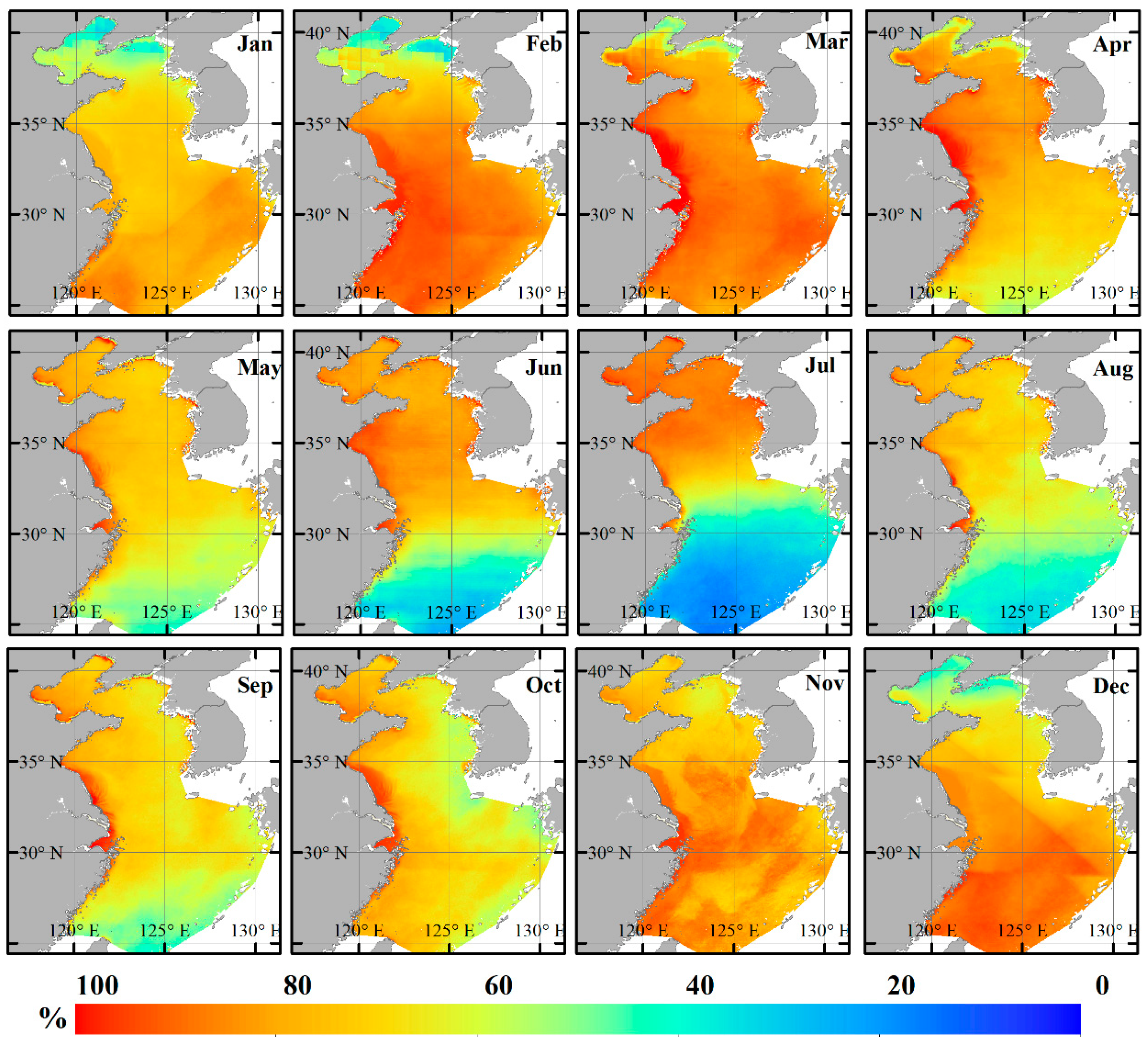
3.1. Cloud Coverage
The spatial distribution and the temporal trend of monthly cloud coverage percentage (CCP) are shown in
Figure 2 and
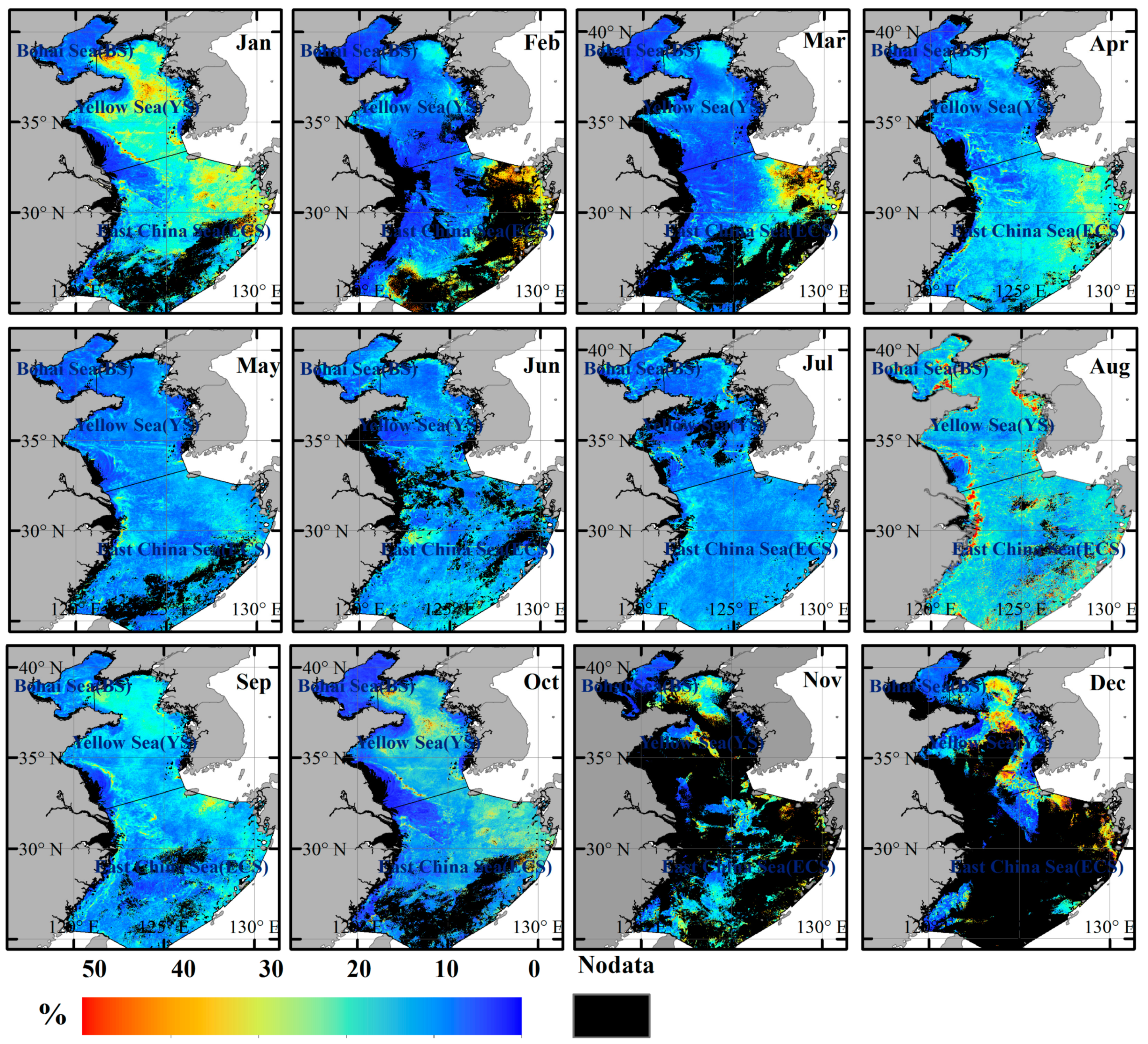
Figure 3. The studied areas demonstrated significant intra-annual variabilities in CCP, both spatially (
Figure 2) and temporally (
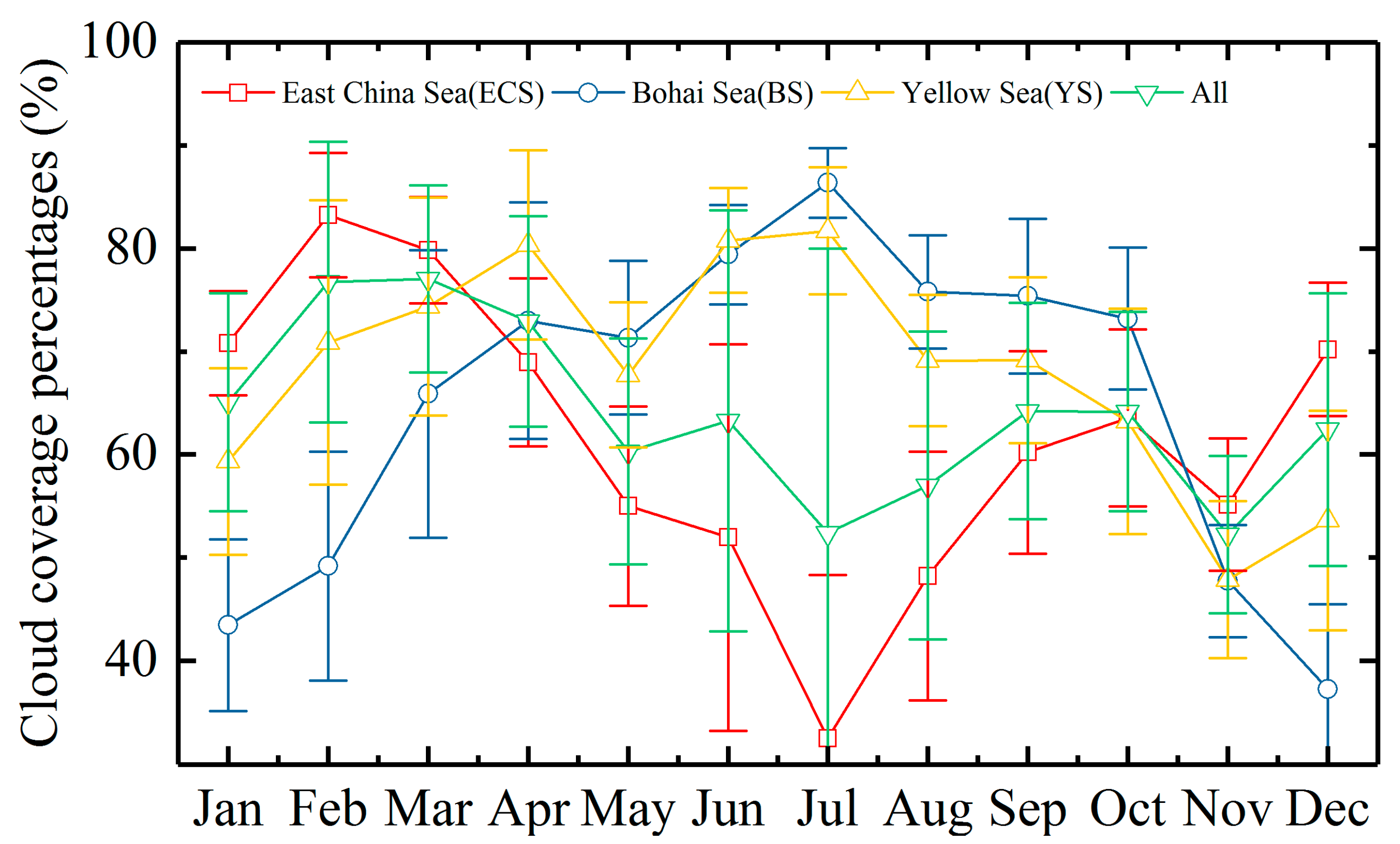
Figure 3). Averaged monthly CCP of the whole study area peaked in March at approximately 77.1%, decreased to the lowest level in July at approximately 52.3%, and then increased again to approximately 72.2% in November. This is consistent with previous results obtained by Xiao et al. [
20], based on merged imagery of daily observations from the SeaWiFS, MODIS, MERIS and VIIRS systems. Obvious monthly CCP patterns were identified for sub-regions of the BS, the YS and the ECS area. The BS and YS areas had similar temporal patterns, with peak CCP in July and lower CCP in December, while an opposite pattern was shown in the ECS region, with low CCP in July and high CCP in December.
The extremely high CCP for the China seas indicates that large portions of the observations from remote-sensing satellites are blinded by clouds. To substantiate this point, the lowest monthly CCP averages for the ECS, BS and YS were found to be 32.5%, 37.3% and 47.9%, equivalently reducing the number of days of cloud-free observations to 20.1, 18.6 and 16, respectively. In the months of the highest CCP, there were only 5, 4 and 5.7 cloud-free days for the ECS, BH and YS area, respectively. The average CCP (standard deviation) values were 62.6% (14.1%), 67.3% (15.5%) and 69.9% (8.6%) for the ECS, BS YS areas, respectively, and it was 65.7% (7.7%) for the whole area. Therefore, it is imperative to understand the effects of the cloud coverage on the remote sensing of TSS in these highly dynamic waters, and to assess the uncertainties in the observations from data from the Terra/Aqua MODI satellite, the most commonly used satellite sensors.
3.2. Biases of TSS Observations
The spatial distribution map of hourly TSS biases was calculated and is presented in
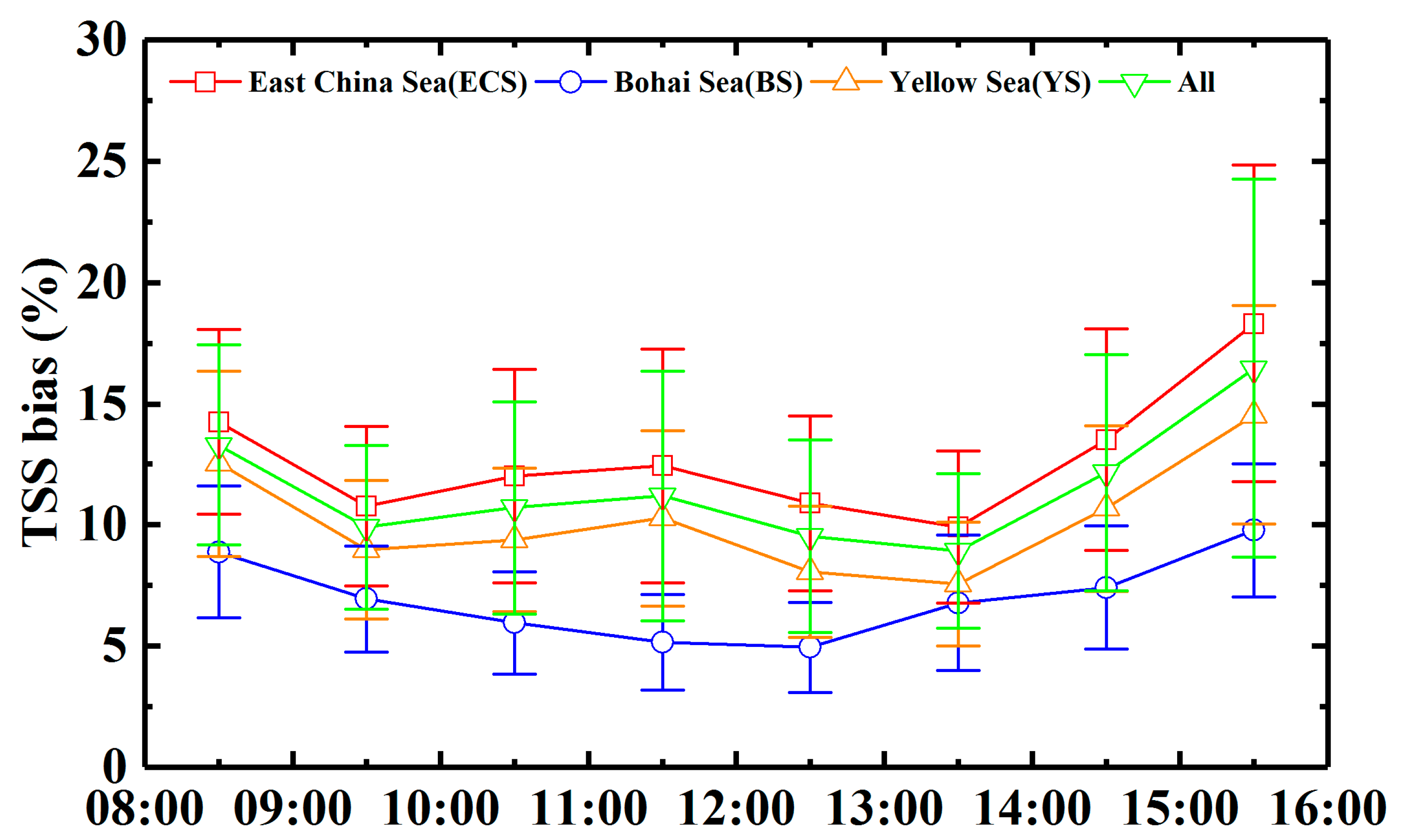
Figure 4, while the statistical results representing the temporal trends for the different regions are illustrated in
Figure 5. TSS bias is the same as P
bias in the following text of the paper. Notable spatial and temporal variations were revealed throughout the Chinese seas. The average (by standard deviation) biases for hourly TSS estimates were 12.8% (2.7%), 7.0% (1.7%), 10.2% (2.3%) and 11.5% (2.5%), in the ECS, BS, YS, and the whole study area, respectively. The results revealed that the maximum TSS bias was as much as 18.3%, 9.8%, 14.5% and 16.5% for the aforementioned sea regions. The largest TSS bias was found in the ECS, while the smallest TSS bias occurred in the BS. The diurnal variation of TSS bias in the whole area shows a decreasing trend from morning, at around 08:30, to the early afternoon, around 13:30 local time. During this period the bias decreased from 13.3% to 8.9%. It then increased to 16.5% at 15:30. Similar diurnal trends were also observed in the ECS, BS and YS.
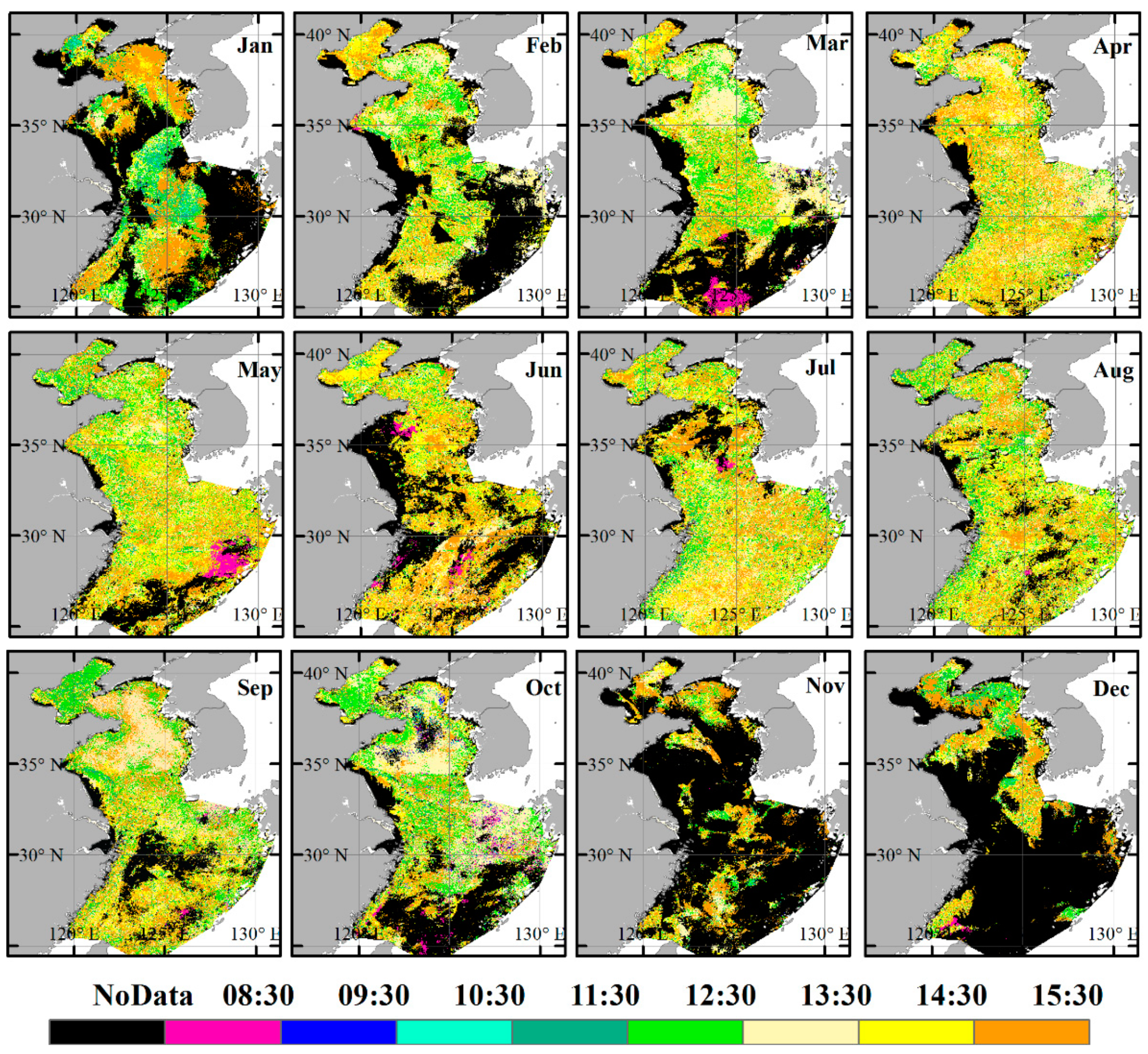
The spatial distributions and temporal trends of the monthly bias for TSS are shown in
Figure 6 and
Figure 7. The pixels that did not satisfy the criterion of eight valid observations a day were labeled as “Nodata” (black color in
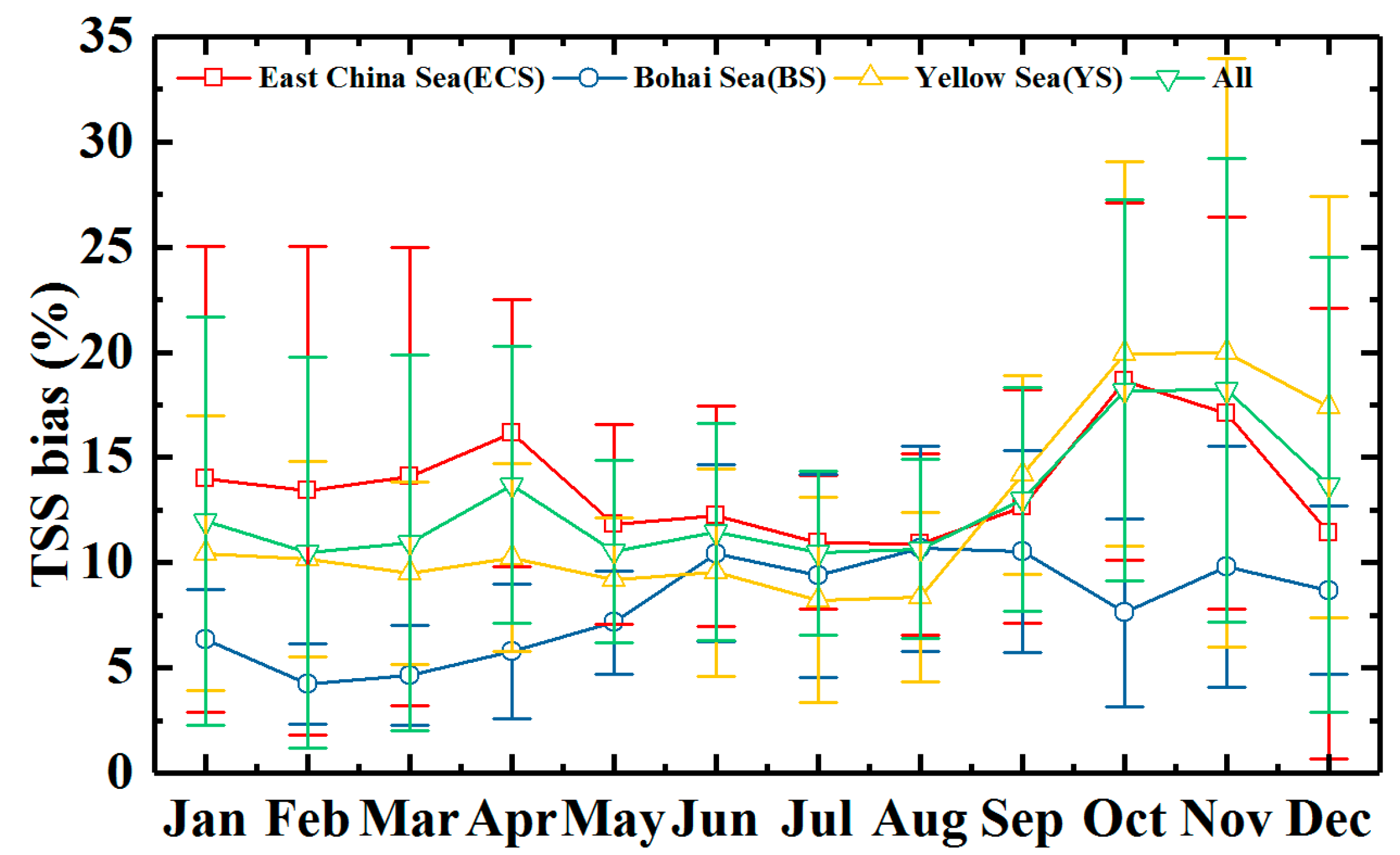
Figure 6) during the statistical analysis. In general, the average monthly bias (±standard deviation) for the TSS was 14.1% (±2.6%), 7.6% (±2.3%) and 12.2% (±4.3%) for the ECS, BS and YS areas respectively, and was 12.8% (±2.7%) for the whole study area.
The maximum monthly bias for TSS was 18.6% and 19.9%, for the ECS and YS in October, and so too was the maximum monthly bias for the whole study area, at 18.2% in October. The maximum monthly bias was 10.7% for the BS region in August. Among the three areas, the YS area had the largest while the BS area had the smallest monthly bias for TSS, and the BS area also showed a smaller overall monthly biases than the other two area.
The changes in monthly bias of TTS, in the ECS and YS, to some extent mirrored that of the whole studied area, with relatively lower biases from May to August, and relatively higher ones from October to December. In comparison, the monthly TSS bias for the BS region displayed almost a reversed pattern, with relatively higher values from June to September, and relatively lower values from October to December and from January to April.
The spatio-temporal variations in monthly TSS biases arise in a manner agreeable with that of the cloud coverage percentage (
Figure 2,
Figure 3,
Figure 6 and
Figure 7). Lower bias values coincided, both temporally and spatially, with higher cloud coverage percentage, and vice versa. For areas with extremely high cloud coverage, such as the majority of the ECS in November and December and the coastal areas of the YS from January to July (
Figure 2), the bias for TSS cannot be calculated due to a lack of valid observations (“Nodata” area in
Figure 6). Consistently, the monthly CCP (the probability of cloud coverage) for these areas in the corresponding months (
Figure 2) was higher than 90%. The changes of monthly TSS bias for the YS area, however, could not be entirely attributed to the cloud coverage over this area, because the changes of monthly biases for TTS did not correlate with the changes of the monthly CCP all year around (
Figure 3 and
Figure 5).
3.3. Factors Affecting TSS Sampling Uncertainties
Two factors were assumed to potentially influence the uncertainties of retrieved TSS values. The first one is the natural variation of TSS itself, as results would be more susceptible to sampling times and frequencies in waters with highly dynamic TSS. In waters with stable TSS, different sampling times and frequencies make no difference to the TSS estimates. In this study, variations of TSS were indicated using the coefficient of variation (CV) to normalize variations across the whole study region, including both highly turbid and relatively clear waters. The second factor is the cloud coverage, which affects the number of valid observations, and thus affects the variations of obtained TSS values over both the short and long term.
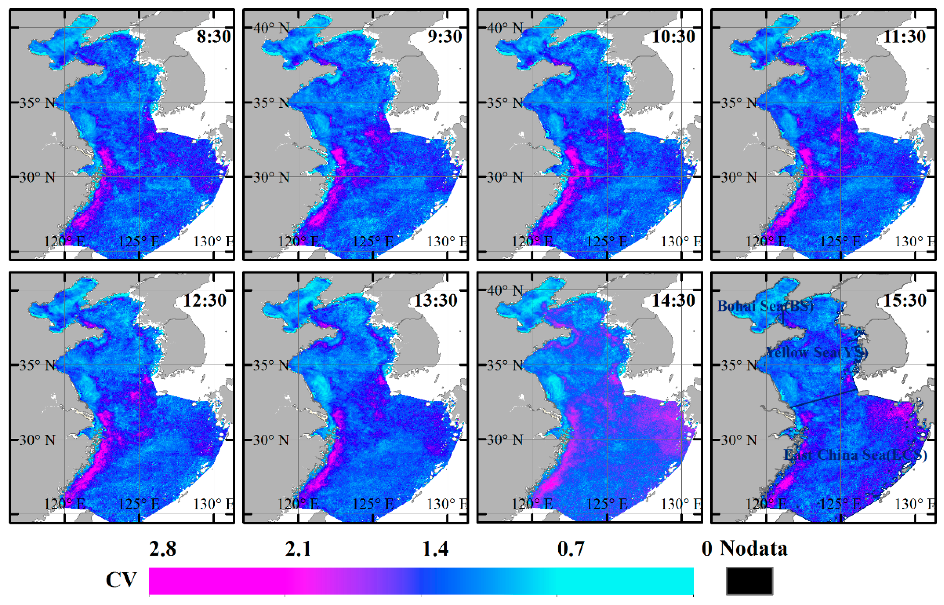
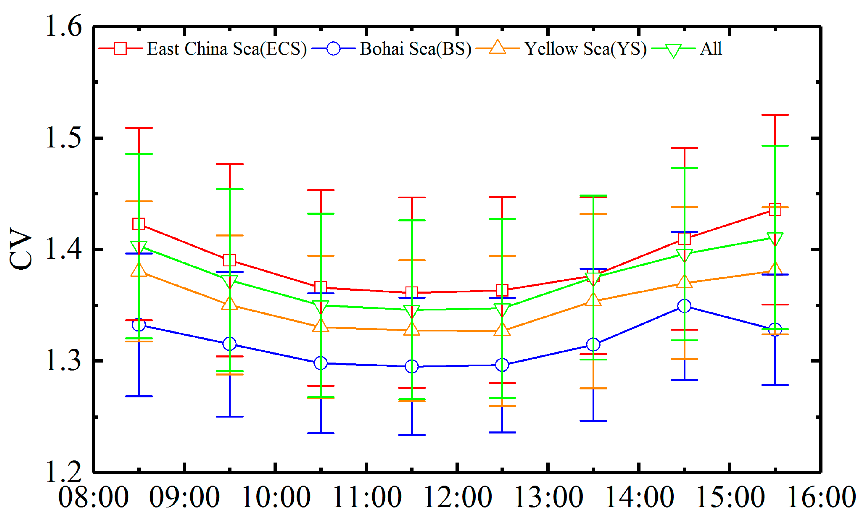
The hourly and monthly trends of TSS CVs across the study areas are presented in
Figure 8,
Figure 9,
Figure 10 and
Figure 11. Significant spatial variations were revealed in the regions of concern at both hourly and monthly scales. At the hourly scale, larger CVs were calculated for offshore waters along the East China Sea (
Figure 8), and the coastal zones of the Bohai and Yellow seas indicated higher temporal variations of TSS levels in these areas; they are dominated by tidal currents that control the sediment transport and resuspension [
51,
53]. Regions with higher TSS bias also displayed larger CVs, which indicates that most of the hourly TSS bias may be due to the TSS variations (
Figure 9). Overall, the temporal trends in the TSS CVs in each subregion were similar to those of the TSS bias, which decreased from morning, around 08:30, to around 13:30 local time, and then increased until 15:30, with the trough found at around 13:30. The magnitudes of the TSS CVs were also consistent with the magnitudes of the TSS bias for the subregions. More specifically, the East China Sea generated the largest TSS bias and CV values, followed by the Yellow Sea. The lowest TSS bias and CV levels were found in the Bohai Sea.
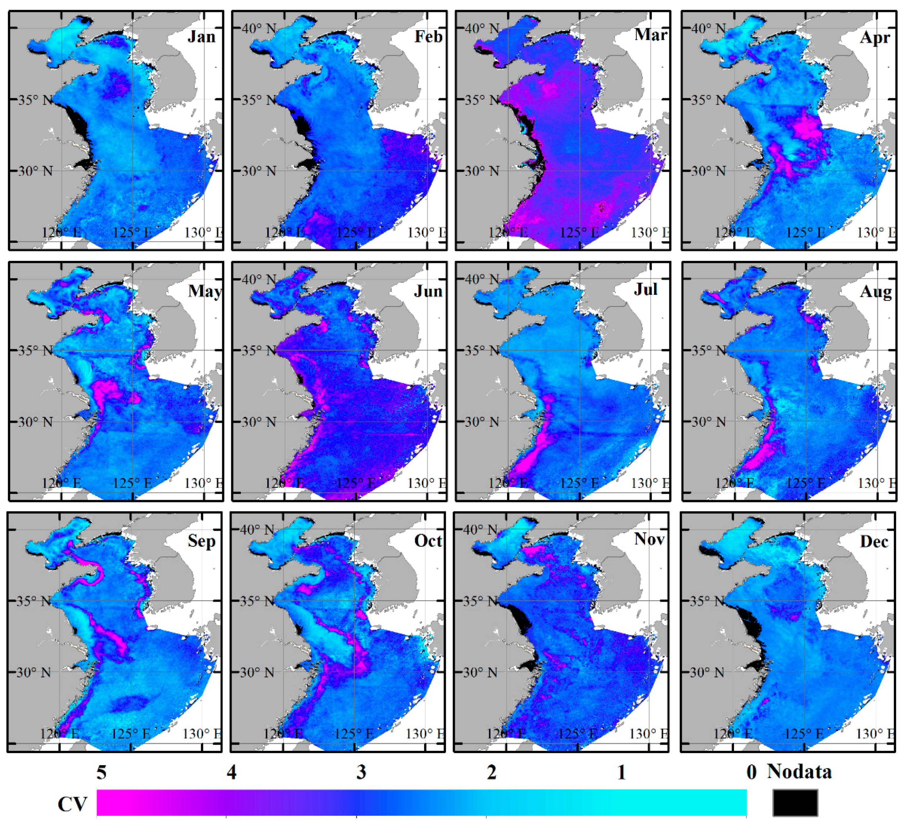
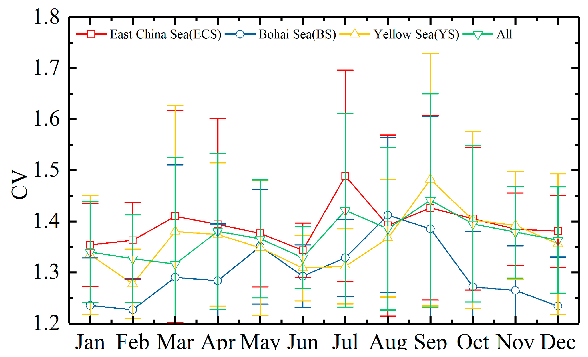
The monthly TSS CV values showed notable spatial and temporal variations (
Figure 10 and
Figure 11). Since CV was determined as the ratio of standard deviation to mean value, areas that experienced high dynamic TSS variations would have higher CV values. Larger CV values were observed along the shorelines of the Yellow Sea and the East China Sea during the summer and autumn seasons, induced by river inflow in the rainy season, whereas the winter season displayed lower CVs. There are evident plumes where the CV differs from surrounding areas, between the coastal regions and the open oceans, which may have been caused by sediment resuspension driven by the combined effects of river discharges, winds, currents and waves in these zones [
54]. Previous studies have demonstrated that suspended matter levels increased significantly from the coastal zones to the open oceans, which were blocked by the warm Taiwan and Kuroshio currents [
55,
56].
The monthly biases and CVs for TSS did not support the hypothesis that the sampling bias was significantly affected by the TSS variations on a monthly scale for the entire study area. Areas with larger biases did not necessarily coincide with higher CV values, and the changing temporal patterns of the two parameters were not consistent either. These results demonstrate that the monthly observations of TSS levels are not solely determined by the TSS variations. Coastal regions with higher CVs were, however, prone to have larger TSS biases.
The results above suggests that both cloud coverage and TSS variations contributed to the TSS sampling biases, spatially and temporally, which indicate that areas with higher cloud coverage or TSS variation are prone to having greater sampling biases. For instance, the TSS biases of the Yellow Sea and East China sea in November, December and January were higher than in other months, which were consistent with the temporal trends of cloud coverages in these areas. But for the Bohai Sea, higher TSS biases were revealed in the summer, and lower ones revealed in the winter, and these coincident with cloud coverage trends in the area. Thus, the sensitivity of the sampling biases to the two factors should be further analyzed.
Maps of the partial correlation of TSS sampling bias with cloud coverage and with TSS CV were obtained at monthly scales, each month using 60 matchups. A correlation greater than 0.6 or 0.8 is generally described as a high or strong correlation, whereas a correlation less than 0.6 is generally described as a weak correlation.
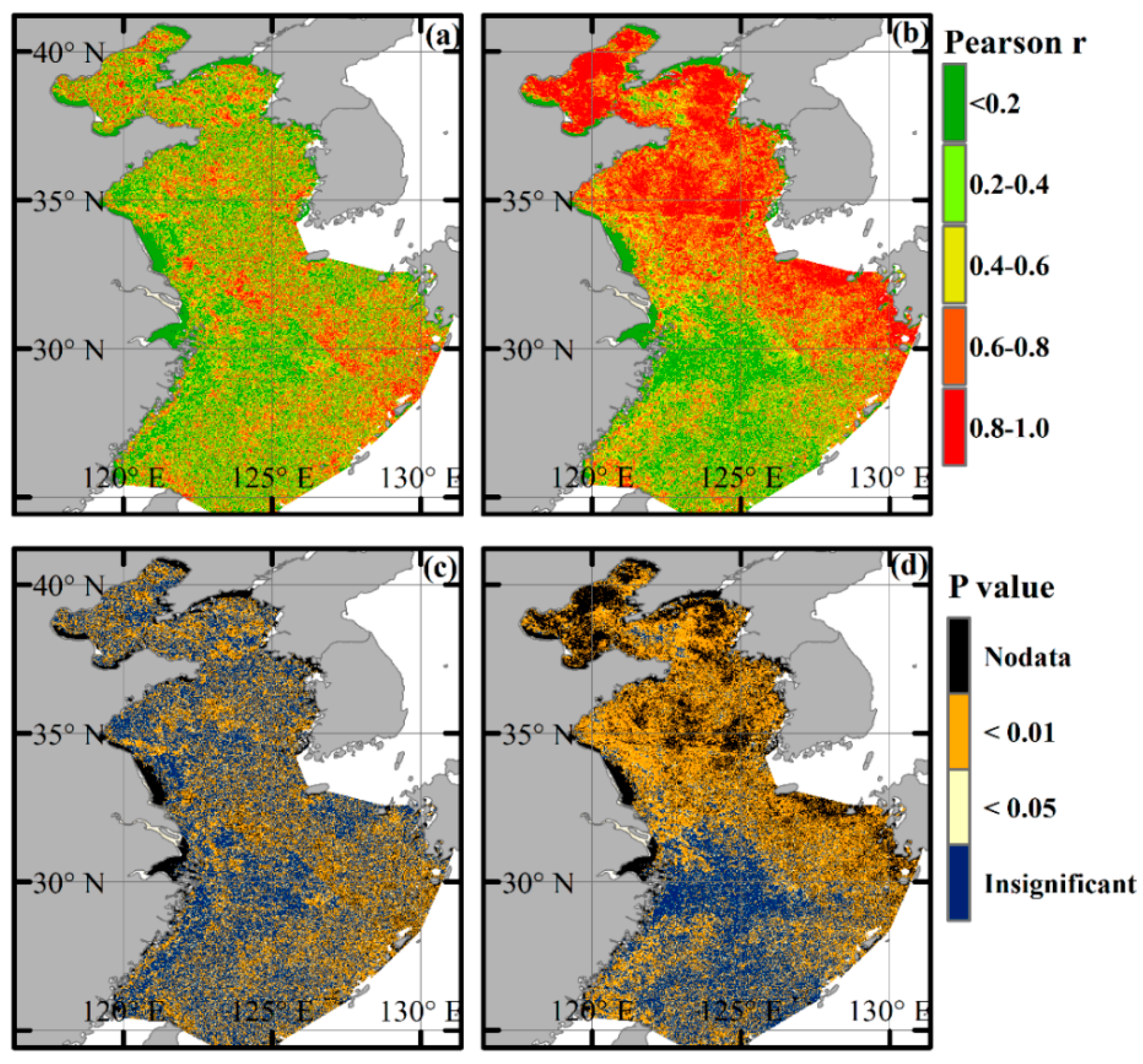
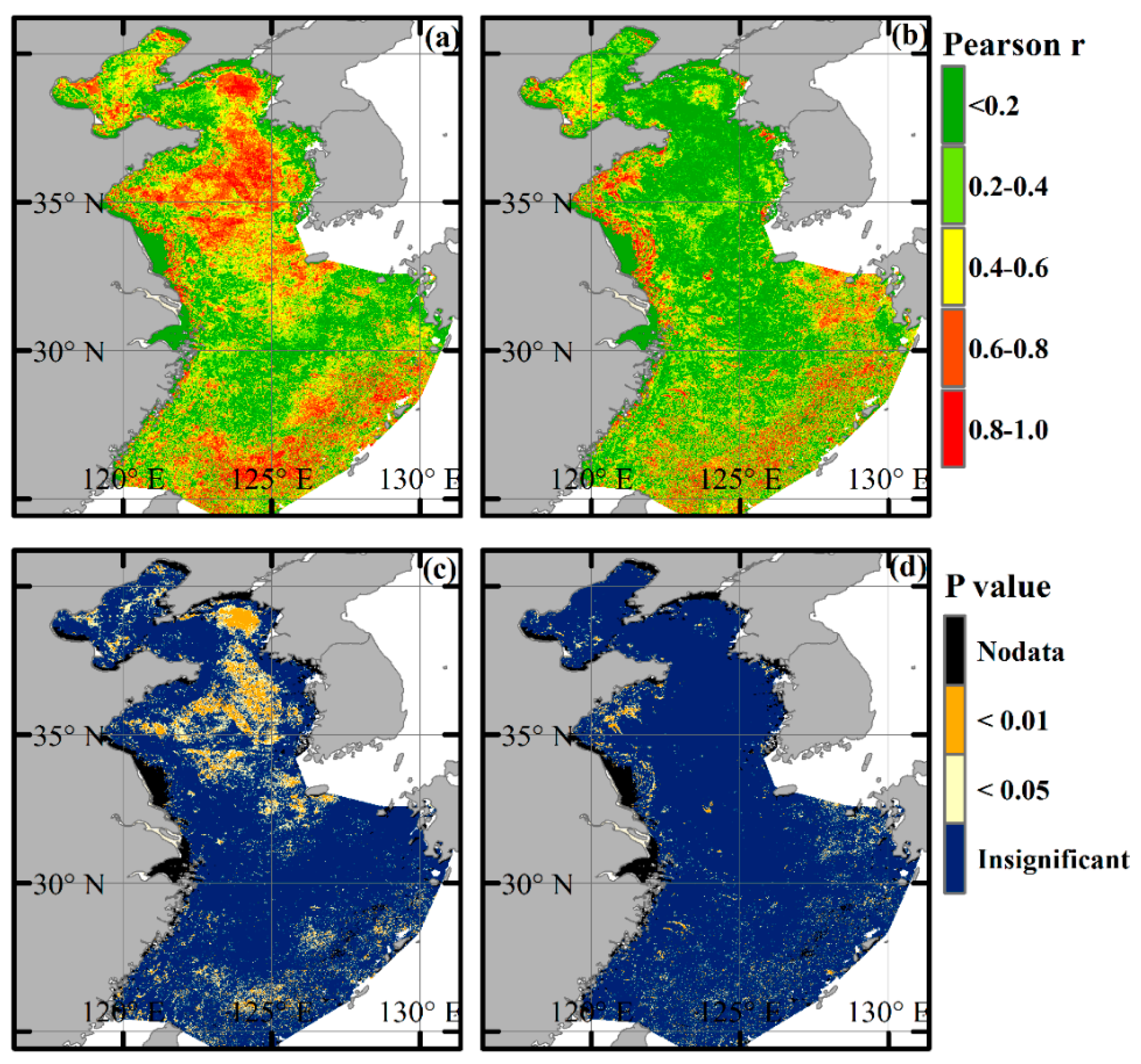
Figure 12 shows the correlations between the hourly TSS sampling biases and the cloud coverage (
Figure 12a) and the TSS CVs (
Figure 12b), together with the
P value maps (
Figure 12c,d). In general, the correlation between the TSS sampling biases and variations was revealed to be higher than that for the relationship between sampling biases and the cloud coverage, at the hourly scale. The results are consistent with the analysis in
Section 3.2 and
Section 4.1, which indicated that the spatial and temporal patterns of hourly scale TSS sampling biases are more closely correlated with the TSS variations than with cloud coverage.
A strong correlation between sampling biases and TSS CVs was found in the Bohai Sea, Yellow Sea, and the northeastern section of the East China Sea, while the rest of the ECS showed a lower correlation, of less than 0.6. A total of 61.6% of the total study area was significantly affected (
P < 0.05) by the TSS variations, while 47.6% was significantly affected by the cloud coverage.
Table 2 presents the area statistics for correlation, and
P values for each subregion. The results clearly showed that the TSS sampling bias is more sensitive to TSS variation than to cloud coverage, for hourly scale observations. For instance, observations for approximately 87% of the Bohai Sea and 86% of the Yellow Sea were significantly affected by the TSS variations. On the contrary, 48.4% and 46.9% of these two subregions were significantly affected by cloud coverage. About half of the area of the East China sea was significantly affected by the TSS variations.
Figure 13 presents maps of correlation for
P values between the monthly bias and the cloud coverage (
Figure 13a,c), and between monthly bias and the TSS CV (
Figure 13b,d). Both the cloud coverage and the TSS variations obviously generated uncertainties in obtaining TSS. For partial areas of the Bohai Gulf, the central Yellow Sea, and the southeastern area of the East China Sea, amounting to 17.1% of the studied areas, sampling bias strongly correlated with cloud coverage. In total, approximately 51.4% of the entire studied region had correlation coefficients higher than 0.6. Areas where TSS variations correlated more closely with sampling biases were found along the coastal regions and in the southeastern area of the East China Sea.
Secondly, the impact of the cloud coverage on sampling biases overshadows that of the TSS variations for monthly observations. At the
P < 0.05 level, 17.6%, 10.9% and 29.5% of the TSS observations in the Bohai Sea, the East China Sea and the Yellow Sea were significantly affected by cloud coverage, respectively, while 4.4%, 6.9% and 4.5% of these seas, in respective order, were significantly affected by TSS variations (
Table 3). It is worth noting that more than 50% of the observations displayed correlation coefficients larger than 0.4 for either cloud coverage or TSS variations. For example, 55% and 60% of the TSS observations in the East China Sea showed
P values greater than 0.4, for cloud coverage and TSS variations, respectively.
3.4. Impacts of Sampling Strategy on Long-Term TSS Trends Monitoring
Time-series of remote sensing data are commonly used for long-term water quality estimations in the regions of interest. Therefore, the impacts of cloud coverage and sampling frequency on sampling uncertainties associated with long-term trends in TSS observations should be resolved. The differences among the TSS time-series retrieved from different satellite sources were examined to determine whether they are consistent regarding the magnitude, seasonality, inter-annual changes and long-term trends, for monthly TSS. To address this, monthly and annual TSS statistics from Terra/MODIS (“simulated” using GOCI 11:30 AM images), Aqua/MODIS (GOCI 13:30 PM images) and Terra/Aqua MODIS (combined observations using GOCI 11:30 and 13:30 images) observations were analyzed and compared to the eight observations of GOCI as references.
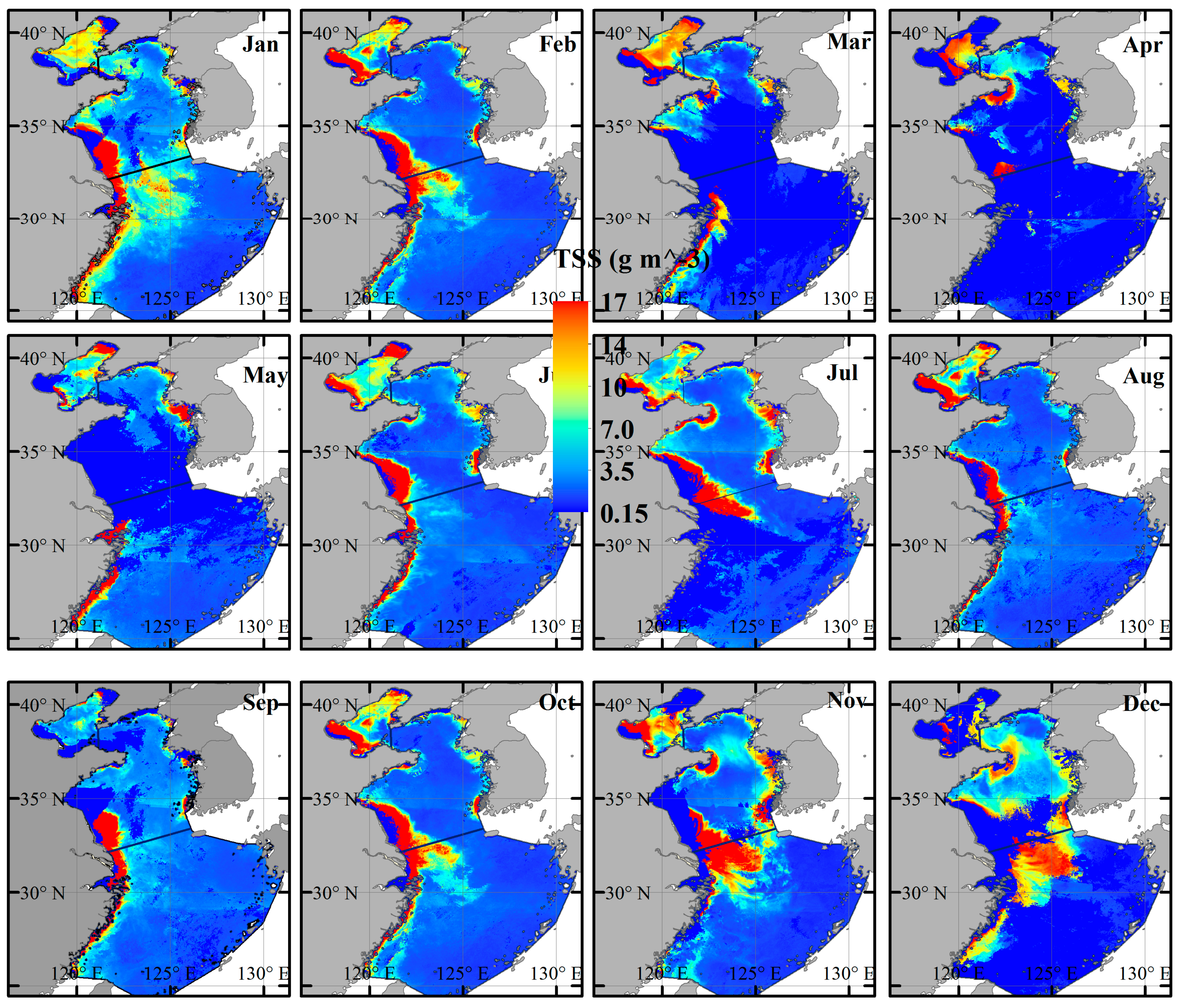
Figure 14 provides the climatology monthly maps of GOCI-observed TSS from 2013 to 2017. The TSS concentrations are higher along the coasts, especially in the Bohai Sea and the Yangtze River estuary, while being lower in the middle of the Yellow Sea and the southeastern area of the East China Sea. From January to March, and October to December, significantly high TSS values (>~10 g/m
3) are observed in most regions of the study area, excluding the middle of the Yellow Sea and the southeastern area of the East China Sea. In general, TSS values are lowest in summer months (July to August), and increase in autumn and winter. These seasonal patterns are consistent with findings in Yuan et al. (2008), whereby the most turbid plumes were observed during winter, and decreased in the following spring and through summer [
57].
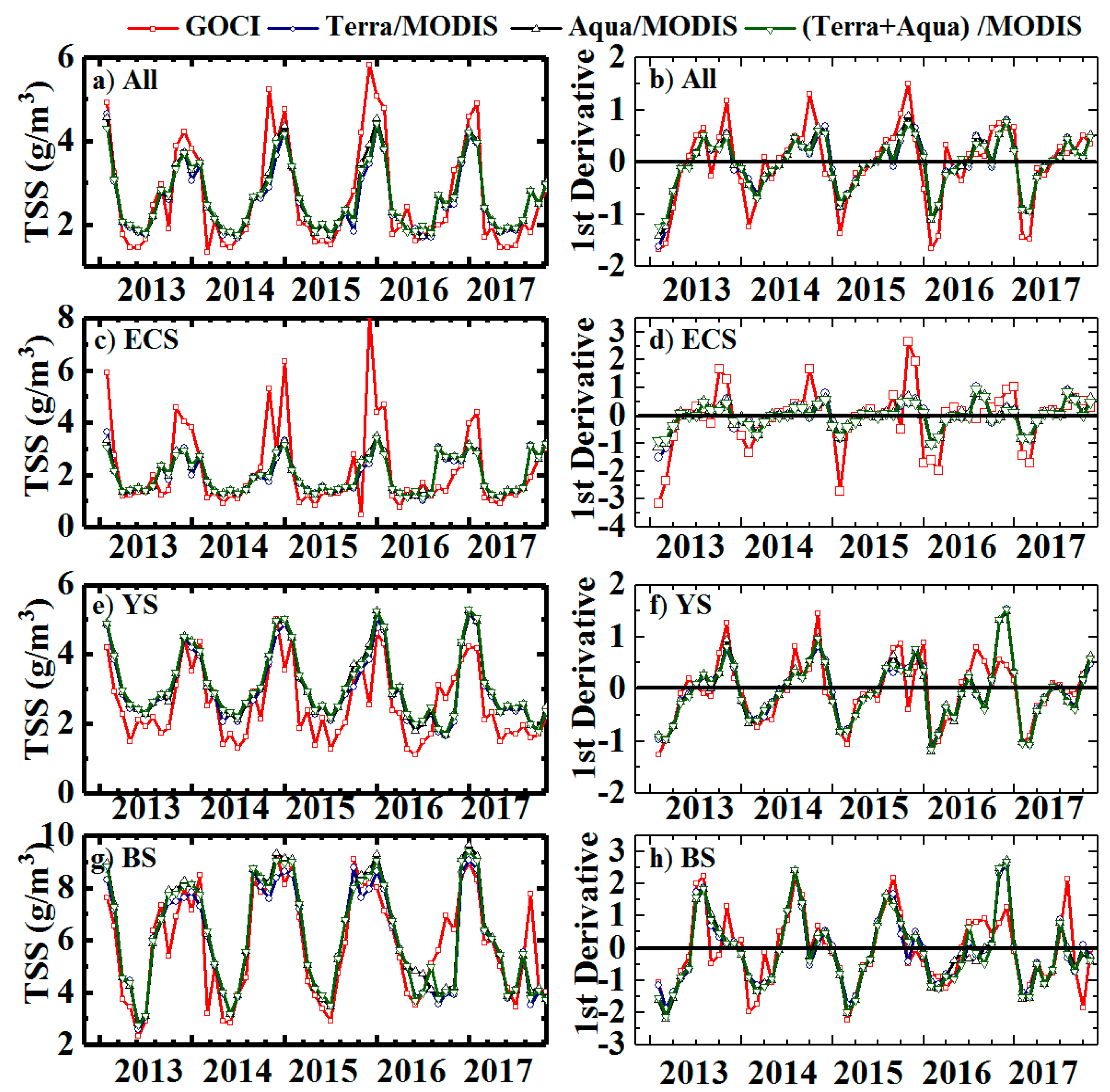
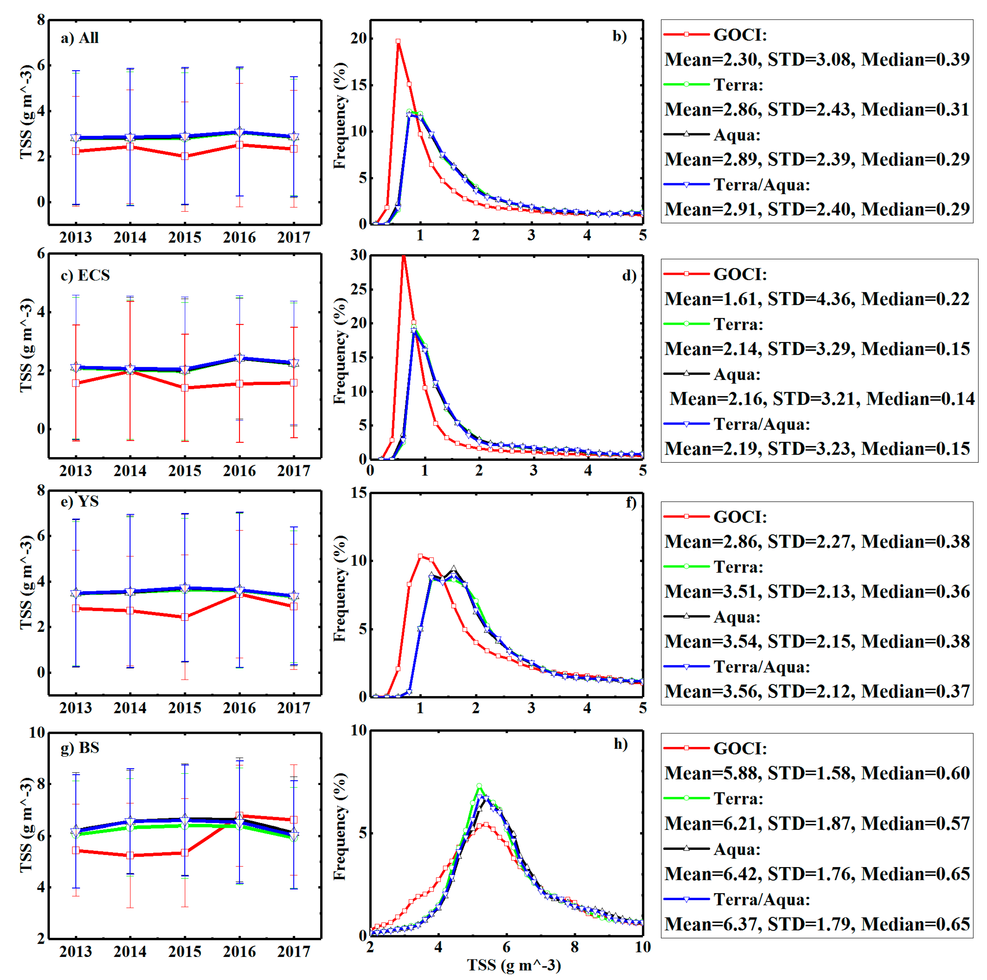
Figure 15 presents the changes of monthly mean TSS from 2013 to 2017, retrieved from GOCI, Terra/MODIS, Aqua/MODIS and Terra/Aqua, for the entire study regions (ALL) and each subregion (ECS, YS, BS). In addition, the first derivative, the instant slope of the tangent line of the TSS-time curve, is presented. In this study, we defined “missed trends” to quantitatively compare the accuracy of different sensors in capturing long-term monthly variations of TSS. First, the baselines of monthly TSS trends were determined using GOCI observations, and the trend between each two months was calculated as the first derivative. A positive derivative signifies an increasing trend, and a negative derivative signifies a decreasing trend, of TSS between each month. Then, the monthly TSS trends from Terra/Aqua MODIS were also calculated and compared to the GOCI results. If the trends observed from GOCI and Terra/Aqua MODIS were opposing, then the numbers of missed trends were added. This process was checked for all months, and the total numbers of missed trends were obtained. Despite the analogous seasonal pattern, significant difference existed in these time-series of monthly TSS.
Specifically, for the whole region, ECS, YS and BS, the ranges of monthly mean TSS obtained from eight GOCI observations were larger than those obtained from one Terra or Aqua/MODIS observation, as well as those from two Terra/Aqua combined observations. For the entire study region, GOCI observations showed a range of 4.47 g/m
3 (with the maximum and minimum TSS of 1.35 and 5.52 g/m
3), whereas the ranges were 2.96, 2.84 and 2.65 g/m
3 for Terra, Aqua and Terra/Aqua MODIS, respectively, as shown in
Table 4. Similar differences were also observed in subregions of the ECS, YS and BS. This inconsistency indicates that single, or a limited number of, observations would miss information on variations of TSS during long-term monitoring, as substantiated by the smaller maximum to minimum ratios in comparison with the eight GOCI observations, as listed in
Table 4. For extremely dynamic waters, as in the ECS [
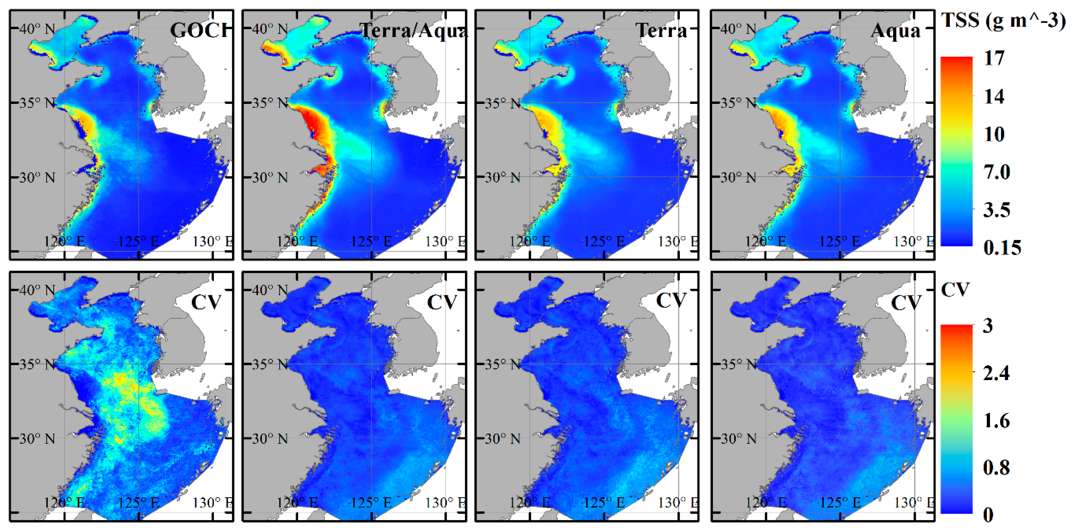
58], the maximum to minimum ratio obtained from GOCI was 16.57, almost five times larger than that for the single daily Terra or Aqua/MODIS observations. The effects of missing information, due to insufficient sampling frequency, on annual TSS variations were also observed, as shown in
Figure 16 and
Figure 17. Larger variations indicated by standard deviation (STD) and CV were revealed from GOCI data, despite similar temporal trends and spatial distributions, compared to Terra/Aqua MODIS data. The higher CV from GOCI observations means more detailed TSS variations were observed from high-frequency remote sensing data. For instance, with eight observations a day, GOCI is able to capture TSS variations within each day, from 8:30 to 15:30, which Tera/Aqua MODIS would have missed. Moreover, the single or combined Terra and Aqua/MODIS seemed to overestimate annual trends of TSS for the entire areas and each subregion.
Another concern when limited numbers of remote-sensing observations were applied for long-term TSS monitoring was the uncaptured tendencies of changes in the time-series, from Terra, Aqua or Terra/Aqua MODIS, at both monthly and annual scales (
Figure 16 and
Figure 17). The tendency of changes between successive months or years could be calculated by the first derivative or slope, as shown in
Figure 17c–h. Differences between derivatives, from Terra, Aqua or Terra/Aqua MODIS time-series, with regard to TSS and the reference GOCI time-series suggested that the tendencies of changes might be omitted for the Terra/Aqua MODIS systems. Since reference GOCI datasets were free of the impacts of different data source, complications resulted from different calibrations, atmospheric corrections, sensitivity drifts or means of data processing. This is evidenced by
Figure 15, the “missed trends” for each region of interest, as comparisons of different time-series to the GOCI reference. In general, approximately 10 monthly tendencies on average were missed in the Terra, Aqua or Terra/Aqua MODIS observations, with the maximum number of 13, and as a consequence, 16.7% of the monthly variations were not captured from 2013 to 2017. Similar results were found at the annual scale, for instance, while an increasing trend from 2013 to 2014 was revealed for the ECS in GOCI observations, a stable or slight decreasing trend was obtained in Terra/Aqua MODIS dataset. Therefore, caution should be taken when limited numbers of observations are used for the monitoring of long-term trends in the water quality parameter, a common approach in ocean color remote-sensing.


