Sampling Uncertainties of Long-Term Remote-Sensing Suspended Sediments Monitoring over China’s Seas: Impacts of Cloud Coverage and Sediment Variations


Abstract
:
1. Introduction
2. Material and Methods
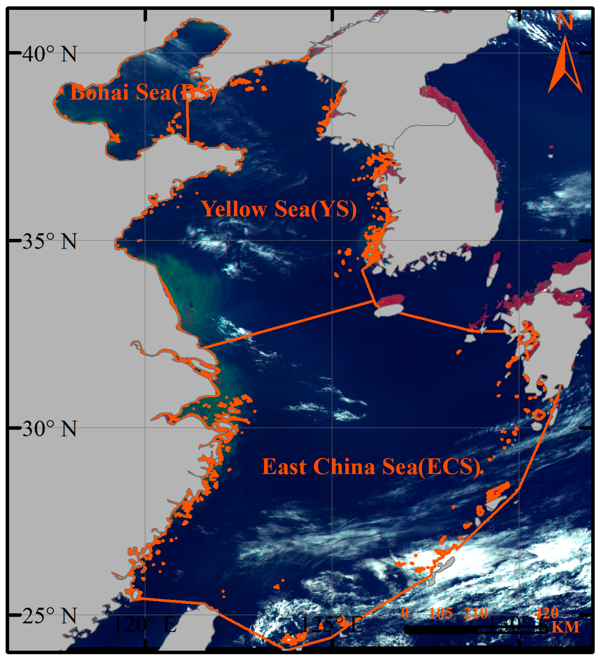
2.1. Study Areas and GOCI Data
2.2. Data Processing
2.3. Cloud Coverage and Total Suspended Sediment Uncertainties Analysis
- (1)
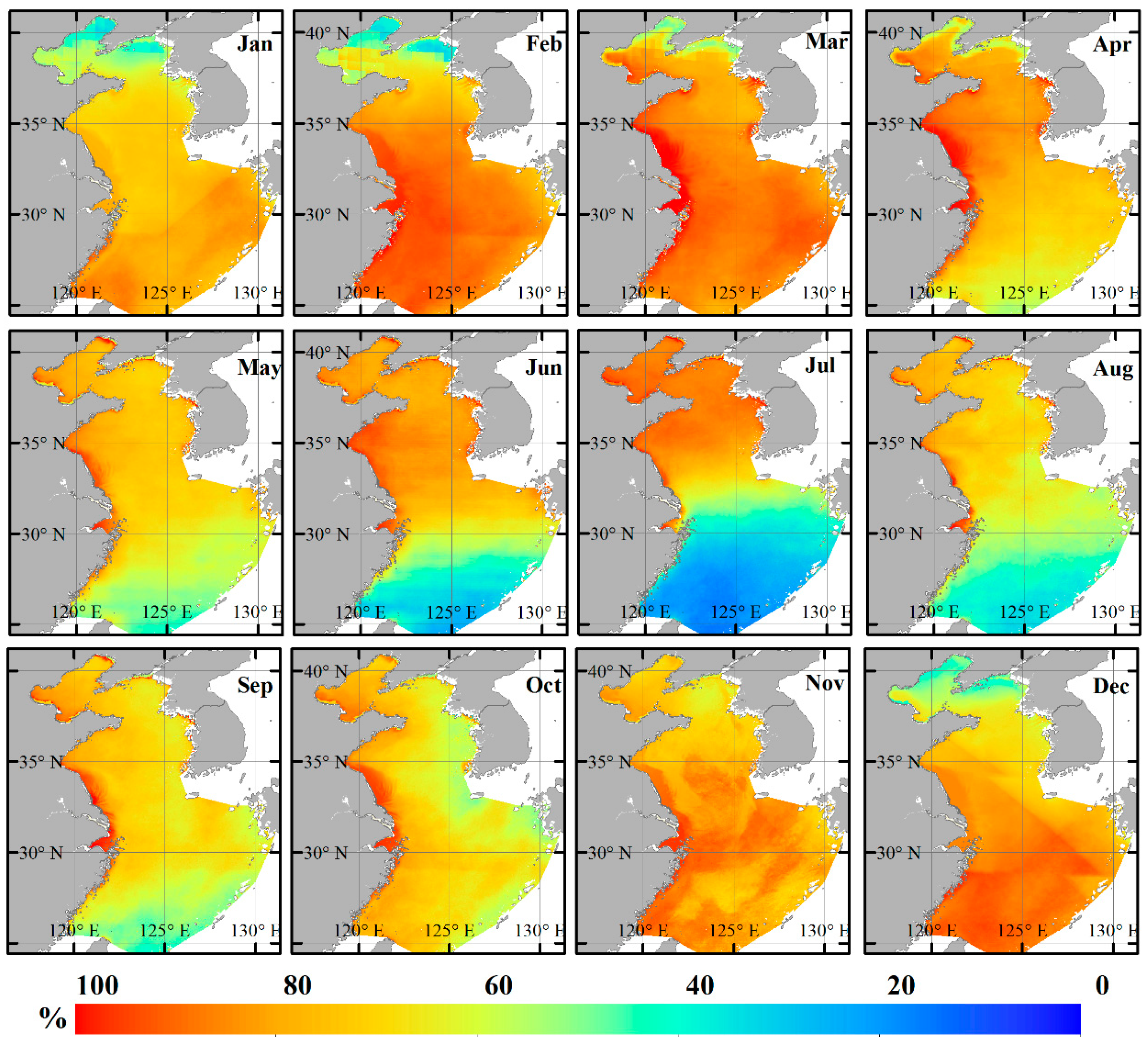
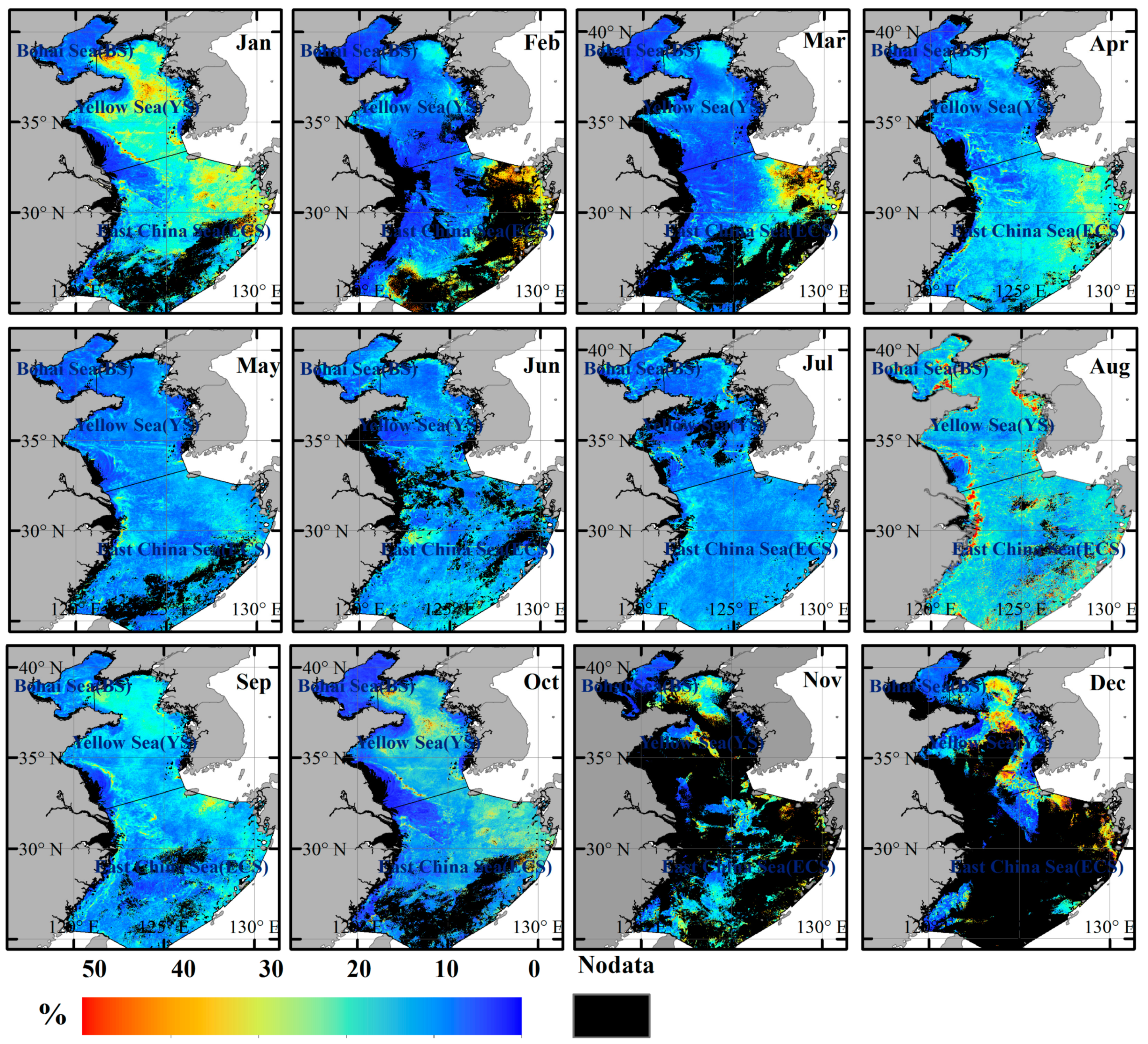
- Cloud statistics: Monthly cloud coverage percentage (CCP) was first calculated for each pixel from five years of GOCI cloud mask data using the ratio of cloud coverage to the total numbers of observations. The spatial and temporal trends of monthly CCP were then obtained.
- (2)
- Estimation of TSS uncertainties: The mean normalized bias (Pbias) of TSS observations due to insufficient sampling rates was estimated using the statistical average of the absolute (unsigned) percentile differences between single observations at each hour h and the daily mean TSS from eight observations. Note that Pbias were only calculated for pixels that satisfy eight valid coverages per day. The value of Pbias was calculated through the following equation:where is the number of valid observations for each pixel from 2013 to 2017, and is the bias for the ith day observation:
2.4. Sensitivity Analysis of TSS Sampling Uncertainties
3. Results
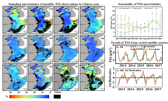
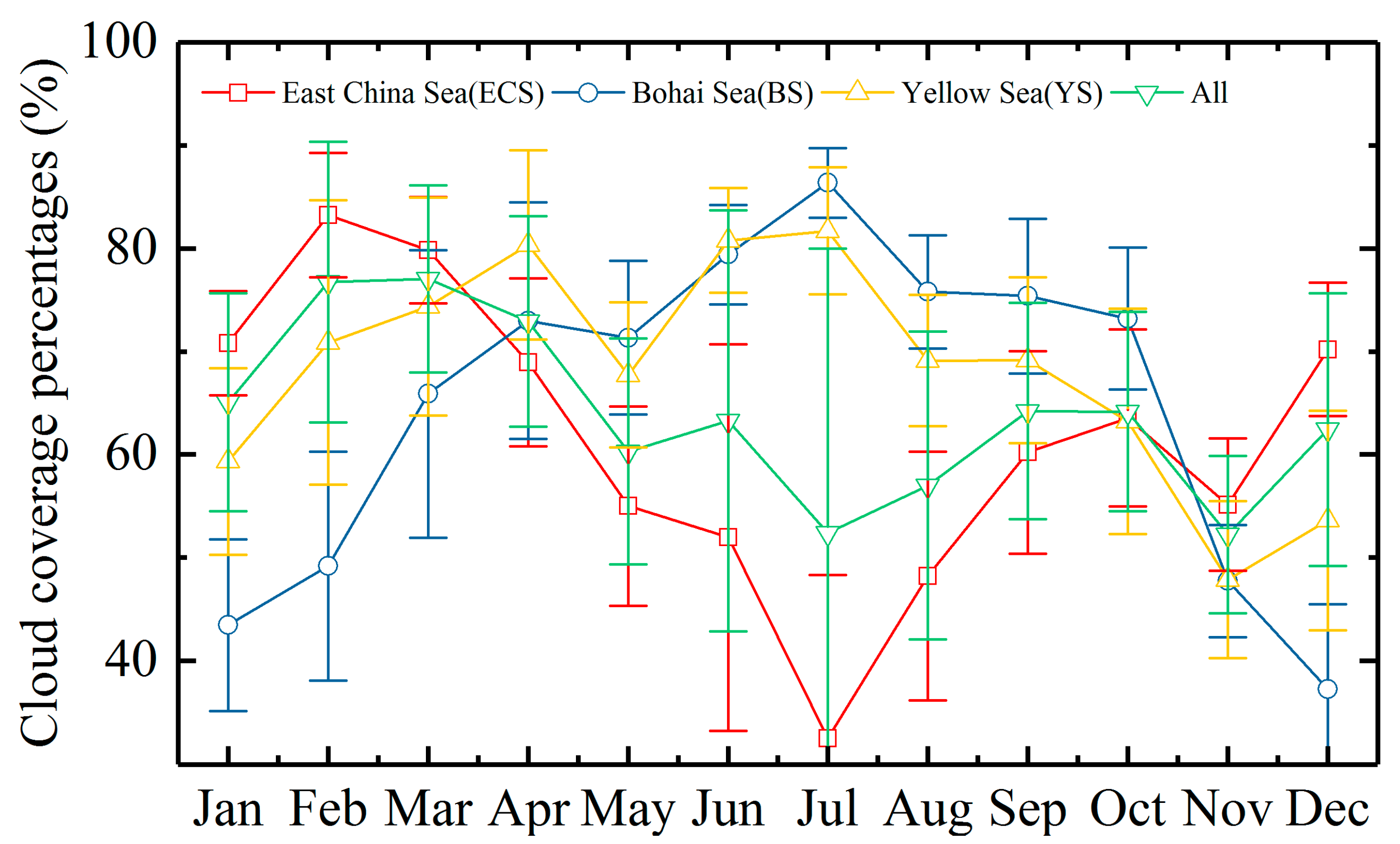
3.1. Cloud Coverage
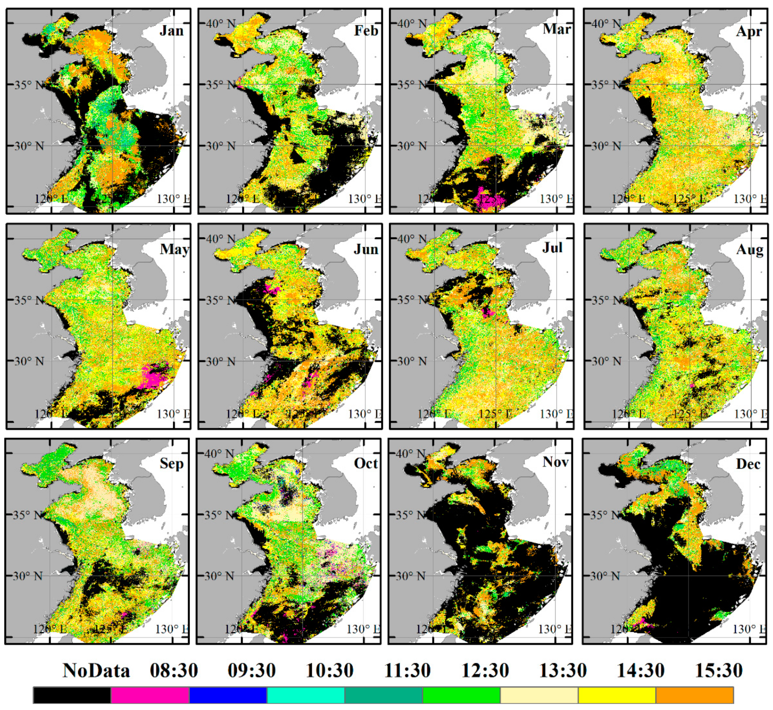
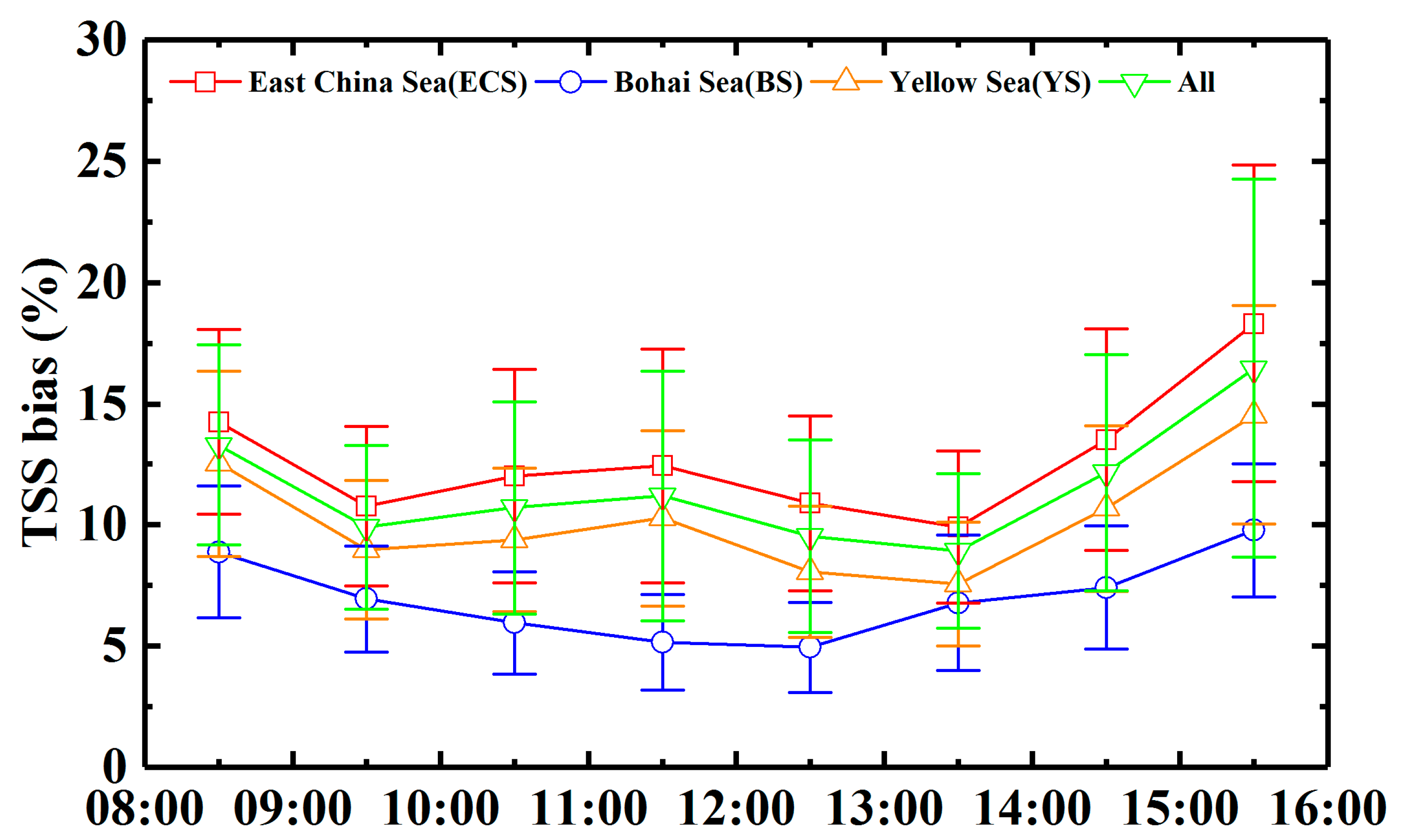
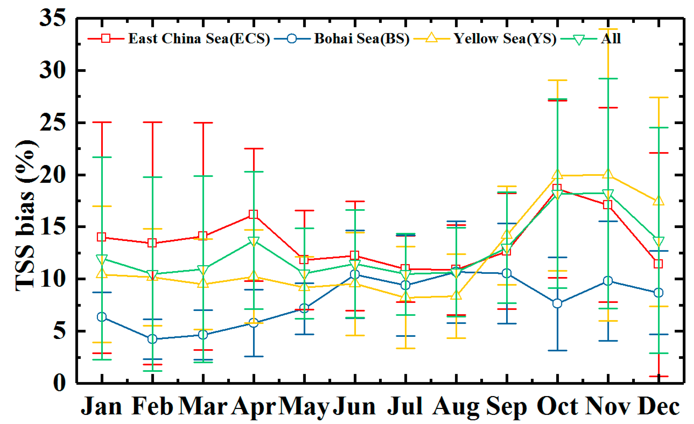
3.2. Biases of TSS Observations
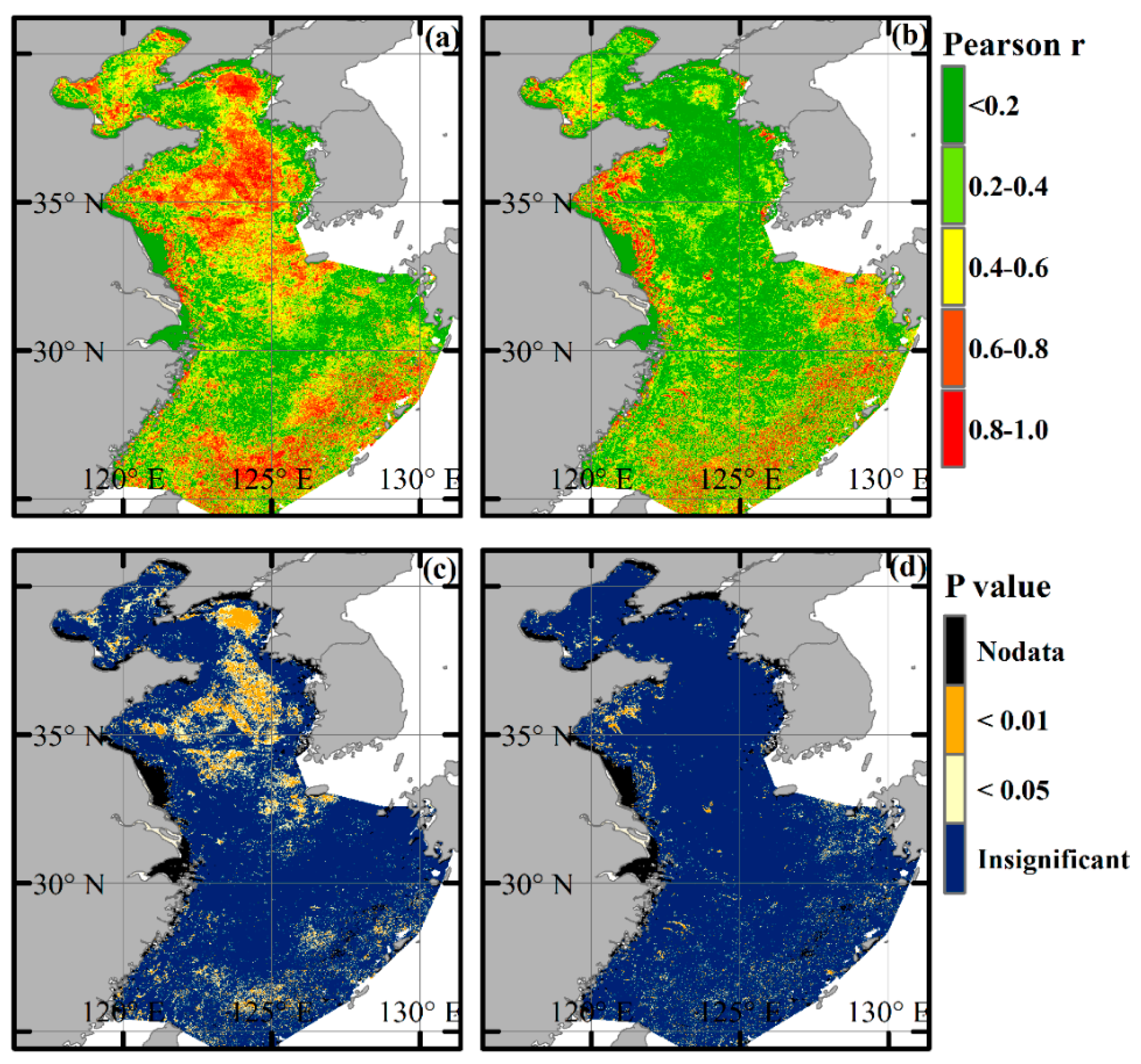
3.3. Factors Affecting TSS Sampling Uncertainties
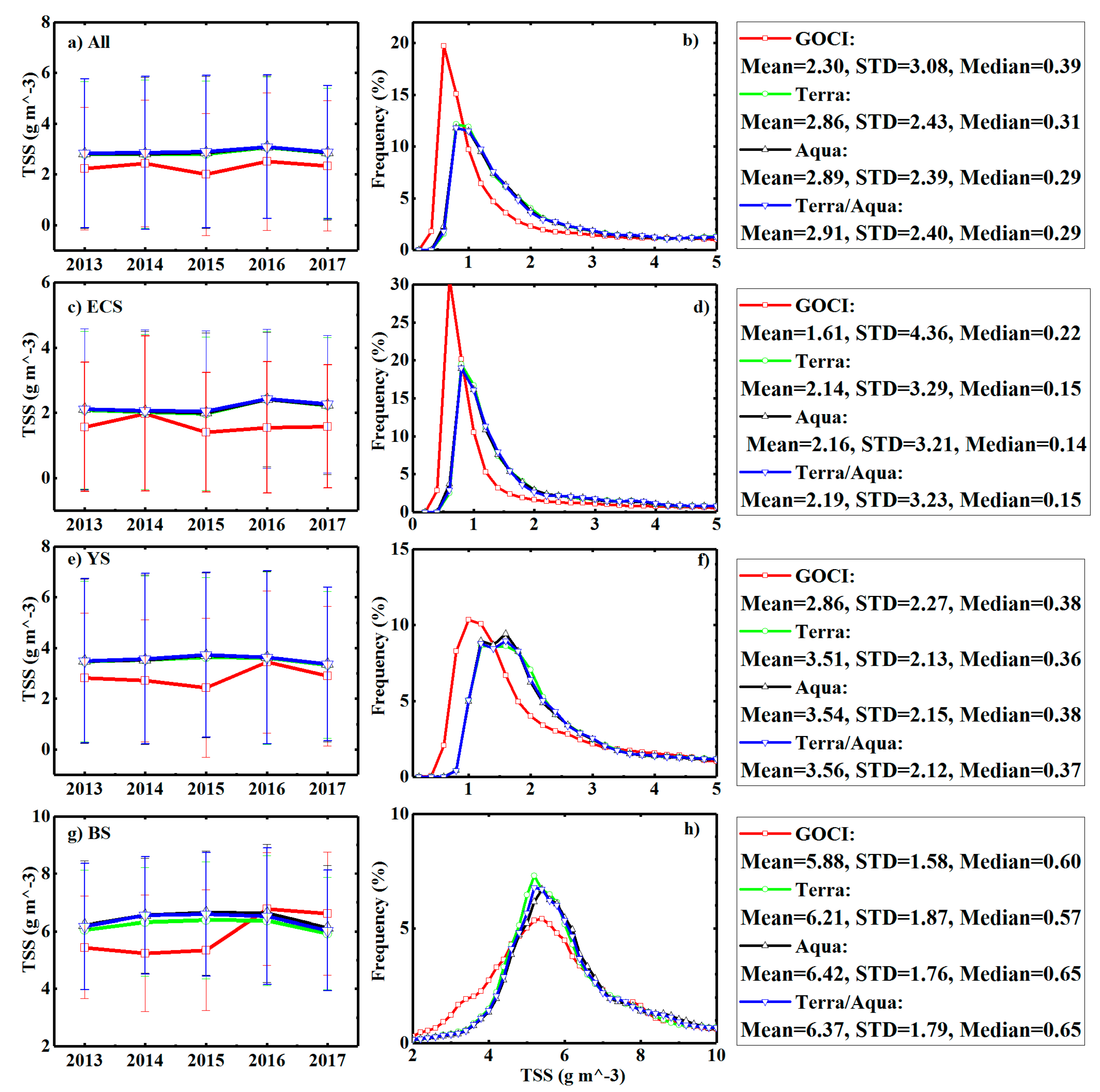
3.4. Impacts of Sampling Strategy on Long-Term TSS Trends Monitoring
4. Discussion
4.1. Advantages of High-Frequency Observations Compared to Conventional Terra/Aqua MODIS
4.2. Implications for Future in situ and Remote Sensing Sampling Strategies
5. Conclusions
Author Contributions
Funding
Conflicts of Interest
References
- Ritchie, J.C.; Zimba, P.V.; Everitt, J.H. Remote Sensing Techniques to Assess Water Quality. Photogramm. Eng. Remote Sens. 2003, 69, 695–704. [Google Scholar] [CrossRef] [Green Version]
- Wang, Y.; Xia, H.; Fu, J.; Sheng, G. Water quality change in reservoirs of shenzhen, China: Detection using landsat/tm data. Sci. Total Environ. 2004, 328, 195. [Google Scholar] [CrossRef] [PubMed]
- Mouw, C.B.; Greb, S.; Aurin, D.; Digiacomo, P.M.; Lee, Z.; Twardowski, M.; Binding, C.; Hu, C.; Ma, R.; Moore, T.; et al. Aquatic color radiometry remote sensing of coastal and inland waters: Challenges and recommendations for future satellite missions. Remote Sens. Environ. 2015, 160, 15–30. [Google Scholar] [CrossRef]
- Feng, L.; Hu, C.; Chen, X.; Cai, X.; Tian, L.; Gan, W. Assessment of inundation changes of Poyang Lake using MODIS observations between 2000 and 2010. Remote Sens. Environ. 2012, 121, 80–92. [Google Scholar] [CrossRef]
- Matthews, M.W.; Bernard, S.; Robertson, L. An algorithm for detecting trophic status (chlorophyll-a), cyanobacterial-dominance, surface scums and floating vegetation in inland and coastal waters. Remote Sens. Environ. 2012, 124, 637–652. [Google Scholar] [CrossRef]
- Mcclain, C.R.; Meister, G. Mission Requirements for Future Ocean-Colour Sensors; International Ocean-Colour Coordinating Group (IOCCG) Report Series, No. 13; IOCCG: Dartmouth, NS, Canada, 2012. [Google Scholar]
- Zhou, Q.; Tian, L.; Wai, O.W.H.; Li, J.; Sun, Z.; Li, W. Impacts of Insufficient Observations on the Monitoring of Short- and Long-Term Suspended Solids Variations in Highly Dynamic Waters, and Implications for an Optimal Observation Strategy. Remote Sens. 2018, 10, 345. [Google Scholar] [CrossRef] [Green Version]
- Gregg, W.W.; Rousseaux, C.S. Simulating PACE Global Ocean Radiances. Front. Mar. Sci. 2017, 4, 2095. [Google Scholar] [CrossRef] [PubMed] [Green Version]
- Hu, C.; Feng, L.; Lee, Z.; Davis, C.O.; Mannino, A.; McClain, C.R.; Franz, B.A. Dynamic range and sensitivity requirements of satellite ocean color sensors: Learning from the past. Appl. Opt. 2012, 51, 6045–6062. [Google Scholar] [CrossRef] [Green Version]
- Maritorena, S.; D’Andon, O.H.F.; Mangin, A.; Siegel, D.A. Merged satellite ocean color data products using a bio-optical model: Characteristics, benefits and issues. Remote Sens. Environ. 2010, 114, 1791–1804. [Google Scholar] [CrossRef]
- Li, J.; Chen, X.; Tian, L.; Huang, J.; Feng, L. Improved capabilities of the Chinese high-resolution remote sensing satellite GF-1 for monitoring suspended particulate matter (SPM) in inland waters: Radiometric and spatial considerations. ISPRS J. Photogramm. Remote Sens. 2015, 106, 145–156. [Google Scholar] [CrossRef]
- Choi, J.-K.; Park, Y.-J.; Ahn, J.-H.; Lim, H.-S.; Eom, J.; Ryu, J.-H. GOCI, the world’s first geostationary ocean color observation satellite, for the monitoring of temporal variability in coastal water turbidity. J. Geophys. Res. Oceans 2012, 117, C09004. [Google Scholar] [CrossRef]
- Ody, A.; Doxaran, D.; Vanhellemont, Q.; Nechad, B.; Novoa, S.; Many, G.; Bourrin, F.; Verney, R.; Pairaud, I.L.; Gentili, B. Potential of High Spatial and Temporal Ocean Color Satellite Data to Study the Dynamics of Suspended Particles in a Micro-Tidal River Plume. Remote Sens. 2016, 8, 245. [Google Scholar] [CrossRef] [Green Version]
- Zolfaghari, K.; Duguay, C. Estimation of Water Quality Parameters in Lake Erie from MERIS Using Linear Mixed Effect Models. Remote Sens. 2016, 8, 473. [Google Scholar] [CrossRef] [Green Version]
- Joshi, I.D.; D’Sa, E.J.; Osburn, C.L.; Bianchi, T.S.; Ko, D.S.; Oviedo-Vargas, D.; Arellano, A.R.; Ward, N. Assessing chromophoric dissolved organic matter (CDOM) distribution, stocks, and fluxes in Apalachicola Bay using combined field, VIIRS ocean color, and model observations. Remote Sens. Environ. 2017, 191, 359–372. [Google Scholar] [CrossRef]
- Concha, J.; Mannino, A.; Franz, B.; Kim, W. Uncertainties in the Geostationary Ocean Color Imager (GOCI) Remote Sensing Reflectance for Assessing Diurnal Variability of Biogeochemical Processes. Remote Sens. 2019, 11, 295. [Google Scholar] [CrossRef] [Green Version]
- Kaufman, Y.J.; Remer, L.A.; Tanre, D.; Li, R.-R.; Kleidman, R.; Mattoo, S.; Levy, R.C.; Eck, T.; Holben, B.; Ichoku, C.; et al. A critical examination of the residual cloud contamination and diurnal sampling effects on MODIS estimates of aerosol over ocean. IEEE Trans. Geosci. Remote Sens. 2005, 43, 2886–2897. [Google Scholar] [CrossRef]
- Racault, M.-F.; Sathyendranath, S.; Platt, T. Impact of missing data on the estimation of ecological indicators from satellite ocean-colour time-series. Remote Sens. Environ. 2014, 152, 15–28. [Google Scholar] [CrossRef] [Green Version]
- Gregg, W.W. Ocean-Colour Data Merging; International Ocean-Colour Coordinating Group: Dartmouth, NS, Canada, 2007. [Google Scholar]
- Yanfang, X.; Jie, Z.; Tingwei, C. Analysis of the effective observation of ocean color satellites of the Yellow and East China Seas. Remote Sens. Lett. 2018, 9, 656–665. [Google Scholar] [CrossRef]
- Feng, L.; Hu, C.; Barnes, B.B.; Mannino, A.; Heidinger, A.; Strabala, K.; Iraci, L.T. Cloud and Sun-glint statistics derived from GOES and MODIS observations over the Intra-Americas Sea for GEO-CAPE mission planning. J. Geophys. Res. Atmos. 2017, 122, 1725–1745. [Google Scholar] [CrossRef]
- Gregg, W.W.; Woodward, R.H. Improvements in coverage frequency of ocean color: Combining data from SeaWiFS and MODIS. IEEE Trans. Geosci. Remote Sens. 1998, 36, 1350–1353. [Google Scholar] [CrossRef]
- Feng, L.; Hu, C. Comparison of Valid Ocean Observations Between MODIS Terra and Aqua Over the Global Oceans. IEEE Trans. Geosci. Remote Sens. 2015, 54, 1575–1585. [Google Scholar] [CrossRef]
- Antoine, D. Ocean-Colour Observations from a Geostationary Orbit; International Ocean-Colour Coordinating Group (IOCCG) Report Series, No. 12; IOCCG: Dartmouth, NS, Canada, 2012. [Google Scholar]
- Gregg, W.W.; Casey, N.W. Sampling biases in MODIS and SeaWiFS ocean chlorophyll data. Remote Sens. Environ. 2007, 111, 25–35. [Google Scholar] [CrossRef] [Green Version]
- Chen, Z.; Hu, C.; Muller-Karger, F.E.; Luther, M.E. Short-term variability of suspended sediment and phytoplankton in Tampa Bay, Florida: Observations from a coastal oceanographic tower and ocean color satellites. Estuar. Coast. Shelf Sci. 2010, 89, 62–72. [Google Scholar] [CrossRef]
- Barnes, B.B.; Hu, C. Cross-Sensor Continuity of Satellite-Derived Water Clarity in the Gulf of Mexico: Insights Into Temporal Aliasing and Implications for Long-Term Water Clarity Assessment. IEEE Trans. Geosci. Remote Sens. 2014, 53, 1761–1772. [Google Scholar] [CrossRef]
- International Ocean-Colour Coordinating Group. Mission Requirements for Future Ocean-Colour Sensors; IOCCG: Dartmouth, NS, Canada, 2013; Volume 13. [Google Scholar]
- Lamquin, N.; Mazeran, C.; Doxaran, D.; Ryu, J.-H.; Park, Y.-J. Assessment of GOCI radiometric products using MERIS, MODIS and field measurements. Ocean Sci. J. 2012, 47, 287–311. [Google Scholar] [CrossRef]
- Moon, J.-E.; Park, Y.-J.; Ryu, J.-H.; Choi, J.-K.; Ahn, J.-H.; Min, J.-E.; Son, Y.-B.; Lee, S.-J.; Han, H.-J.; Ahn, Y.-H. Initial validation of GOCI water products against in situ data collected around Korean peninsula for 2010–2011. Ocean Sci. J. 2012, 47, 261–277. [Google Scholar] [CrossRef]
- Qiu, Z.; Zheng, L.; Zhou, Y.; Sun, D.; Wang, S.; Wu, W. Innovative GOCI algorithm to derive turbidity in highly turbid waters: A case study in the Zhejiang coastal area. Opt. Express 2015, 23, A1179–A1193. [Google Scholar] [CrossRef]
- Kang, G.; Coste, P.; Youn, H.; Faure, F.; Choi, S. An In-Orbit Radiometric Calibration Method of the Geostationary Ocean Color Imager. IEEE Trans. Geosci. Remote Sens. 2010, 48, 4322–4328. [Google Scholar] [CrossRef]
- Ryu, J.-H.; Han, H.-J.; Cho, S.; Park, Y.-J.; Ahn, Y.-H. Overview of geostationary ocean color imager (GOCI) and GOCI data processing system (GDPS). Ocean Sci. J. 2012, 47, 223–233. [Google Scholar] [CrossRef]
- Qin, Y. Study of influence of sediment loads discharged from huanghe river on sedimentation in bonhai sea and huanghe sea. In Proceedings of the International Symposium on “Sedimentation on the Continental Shelf with Special Reference to the East China Sea”, Yantai, China, 16 January 1983; pp. 56–79. [Google Scholar]
- Wang, H.; Wang, A.; Bi, N.; Zeng, X.; Xiao, H. Seasonal distribution of suspended sediment in the Bohai Sea, China. Cont. Shelf Res. 2014, 90, 17–32. [Google Scholar] [CrossRef]
- Yang, Z.; Ji, Y.; Bi, N.; Lei, K.; Wang, H. Sediment transport off the Huanghe (Yellow River) delta and in the adjacent Bohai Sea in winter and seasonal comparison. Estuar. Coast. Shelf Sci. 2011, 93, 173–181. [Google Scholar] [CrossRef]
- Wang, H.; Bi, N.; Saito, Y.; Wang, Y.; Sun, X.; Zhang, J.; Yang, Z. Recent changes in sediment delivery by the Huanghe (Yellow River) to the sea: Causes and environmental implications in its estuary. J. Hydrol. 2010, 391, 302–313. [Google Scholar] [CrossRef]
- Tang, Q.; Wang, S.; Qiu, Z.; Sun, D.; Bilal, M. Variability of the Suspended Particle Cross-Sectional Area in the Bohai Sea and Yellow Sea. Remote Sens. 2019, 11, 1187. [Google Scholar] [CrossRef] [Green Version]
- Bao, X.; Li, Z.; Wang, Y.; Li, N. Sediment distribution features in the north yellow sea during summer and winter. J. Sediment Res. 2010, 2, 48–56. [Google Scholar]
- Yu, L.-L.; Jiang, W.-S. Seasonal variations in the distributions of suspended fine particulate matter in the yellow sea and the east china sea. Oceanol. Limnol. Sin. 2011, 42, 474–481. [Google Scholar]
- Dong, L.; Guan, W.; Chen, Q.; Li, X.; Liu, X.; Zeng, X. Sediment transport in the Yellow Sea and East China Sea. Estuar. Coast. Shelf Sci. 2011, 93, 248–258. [Google Scholar] [CrossRef]
- Liu, Z.-X.; Berné, S.; Saito, Y.; Lericolais, G.; Marsset, T. Quaternary seismic stratigraphy and paleoenvironments on the continental shelf of the East China Sea. J. Asian Earth Sci. 2000, 18, 441–452. [Google Scholar] [CrossRef]
- Hu, C.; Feng, L.; Lee, Z. Evaluation of GOCI sensitivity for At-Sensor radiance and GDPS-Retrieved chlorophyll-a products. Ocean Sci. J. 2012, 47, 279–285. [Google Scholar] [CrossRef]
- Ahn, J.-H.; Park, Y.-J.; Kim, W.; Lee, B. Simple aerosol correction technique based on the spectral relationships of the aerosol multiple-scattering reflectances for atmospheric correction over the oceans. Opt. Express 2016, 24, 29659. [Google Scholar] [CrossRef]
- Ahn, J.-H.; Park, Y.-J.; Ryu, J.-H.; Lee, B.; Oh, I.S. Development of atmospheric correction algorithm for Geostationary Ocean Color Imager (GOCI). Ocean Sci. J. 2012, 47, 247–259. [Google Scholar] [CrossRef]
- Siswanto, E.; Tang, J.; Yamaguchi, H.; Ahn, Y.-H.; Ishizaka, J.; Yoo, S.; Kim, S.-W.; Kiyomoto, Y.; Yamada, K.; Chiang, C.; et al. Empirical ocean-color algorithms to retrieve chlorophyll-a, total suspended matter, and colored dissolved organic matter absorption coefficient in the Yellow and East China Seas. J. Oceanogr. 2011, 67, 627–650. [Google Scholar] [CrossRef]
- Min, J.; Choi, J.-K.; Park, Y.; Ryu, J.H. In Retrieval of Suspended Sediment Concentration in the Coastal Waters of Yellow Sea from Geostationary Ocean Color Imager (goci). In Proceedings of the International Symposium on Remote Sensing, Chiba, Japan, 10 May 2013; pp. 15–17. [Google Scholar]
- Ruddick, K.G.; Vanhellemont, Q.; Yan, J.; Neukermans, G.; Wei, G.; Shang, S. Variability of suspended particulate matter in the Bohai Sea from the geostationary Ocean Color Imager (GOCI). Ocean Sci. J. 2012, 47, 331–345. [Google Scholar] [CrossRef]
- Choi, J.-K.; Yang, H.; Han, H.-J.; Ryu, J.-H.; Park, Y.-J. Quantitative estimation of suspended sediment movements in coastal region using GOCI. J. Coast. Res. 2013, 165, 1367–1372. [Google Scholar] [CrossRef]
- Wang, M.; Ahn, J.-H.; Jiang, L.; Shi, W.; Son, S.; Park, Y.-J.; Ryu, J.-H. Ocean color products from the Korean Geostationary Ocean Color Imager (GOCI). Opt. Express 2013, 21, 3835–3849. [Google Scholar] [CrossRef] [PubMed]
- Son, S.; Kim, Y.-H.; Kwon, J.-I.; Kim, H.-C.; Park, K.-S. Characterization of spatial and temporal variation of suspended sediments in the Yellow and East China Seas using satellite ocean color data. GISci. Remote Sens. 2014, 51, 212–226. [Google Scholar] [CrossRef]
- Park, Y.J.; Ahn, Y.H.; Han, H.; Yang, H.; Moon, J.; Ahn, J.; Lee, B.; Min, J.; Lee, S.; Kim, K.; et al. Goci Level 2 Ocean Color Products Brief Algorithm Description. Available online: http://kosc.kiost.ac.kr/download.php?fileName=ATBD_master_v9_1.pdf (accessed on 12 April 2015).
- Lee, H.J.; Park, J.Y.; Lee, S.H.; Lee, J.M.; Kim, T.K. Suspended Sediment Transport in a Rock-Bound, Macrotidal Estuary: Han Estuary, Eastern Yellow Sea. J. Coast. Res. 2013, 29, 358–371. [Google Scholar] [CrossRef]
- Wang, W.; Jiang, W. Study on the seasonal variation of the suspended sediment distribution and transportation in the East China Seas based on SeaWiFS data. J. Ocean Univ. China 2008, 7, 385–392. [Google Scholar] [CrossRef]
- Chen, J.; Liu, J. The spatial and temporal changes of chlorophyll-a and suspended matter in the eastern coastal zones of china during 1997–2013. Cont. Shelf Res. 2015, 95, 89–98. [Google Scholar] [CrossRef]
- Bian, C.; Jiang, W.; Quan, Q.; Wang, T.; Greatbatch, R.J.; Li, W. Distributions of suspended sediment concentration in the Yellow Sea and the East China Sea based on field surveys during the four seasons of 2011. J. Mar. Syst. 2013, 121, 24–35. [Google Scholar] [CrossRef]
- Yuan, D.; Zhu, J.; Li, C.; Hu, D. Cross-shelf circulation in the Yellow and East China Seas indicated by MODIS satellite observations. J. Mar. Syst. 2008, 70, 134–149. [Google Scholar] [CrossRef]
- He, X.; Bai, Y.; Pan, D.; Huang, N.; Dong, X.; Chen, J.; Chen, C.-T.A.; Cui, Q. Using geostationary satellite ocean color data to map the diurnal dynamics of suspended particulate matter in coastal waters. Remote Sens. Environ. 2013, 133, 225–239. [Google Scholar] [CrossRef]


| East China Sea (ECS) | Bohai Sea (BS) | Yellow Sea (YS) | |
|---|---|---|---|
| January | 29.21 | 56.52 | 40.64 |
| February | 16.76 | 50.81 | 29.11 |
| March | 20.15 | 34.07 | 25.59 |
| April | 31.05 | 26.98 | 19.63 |
| May | 45.01 | 28.66 | 32.25 |
| June | 48.04 | 20.60 | 19.22 |
| July | 67.47 | 13.63 | 18.30 |
| August | 51.78 | 24.19 | 30.87 |
| September | 39.78 | 24.60 | 30.84 |
| October | 36.44 | 26.78 | 36.74 |
| November | 44.86 | 52.26 | 52.12 |
| December | 29.79 | 62.70 | 46.36 |
| P Value | Bohai | East China Sea | Yellow Sea | All | |
|---|---|---|---|---|---|
| Cloud impacts | P < 0.01 | 35.20% | 34.60% | 33.50% | 34.30% |
| P < 0.05 | 48.40% | 47.80% | 46.90% | 47.60% | |
| CV impacts | P < 0.01 | 79.80% | 37.80% | 77.90% | 50.20% |
| P < 0.05 | 86.90% | 50.60% | 86.10% | 61.60% |
| P Value | Bohai | East China Sea | Yellow Sea | All | |
|---|---|---|---|---|---|
| Cloud impacts | P < 0.01 | 3.50% | 2.90% | 10.90% | 5.50% |
| P < 0.05 | 17.60% | 10.90% | 29.50% | 17.10% | |
| CV impacts | P < 0.01 | 0.90% | 1.90% | 1.60% | 1.70% |
| P < 0.05 | 4.40% | 6.90% | 4.50% | 5.80% |
| Minimum | Median | Maximum | Range | Max/Min Ratio | Missed Trends | ||
|---|---|---|---|---|---|---|---|
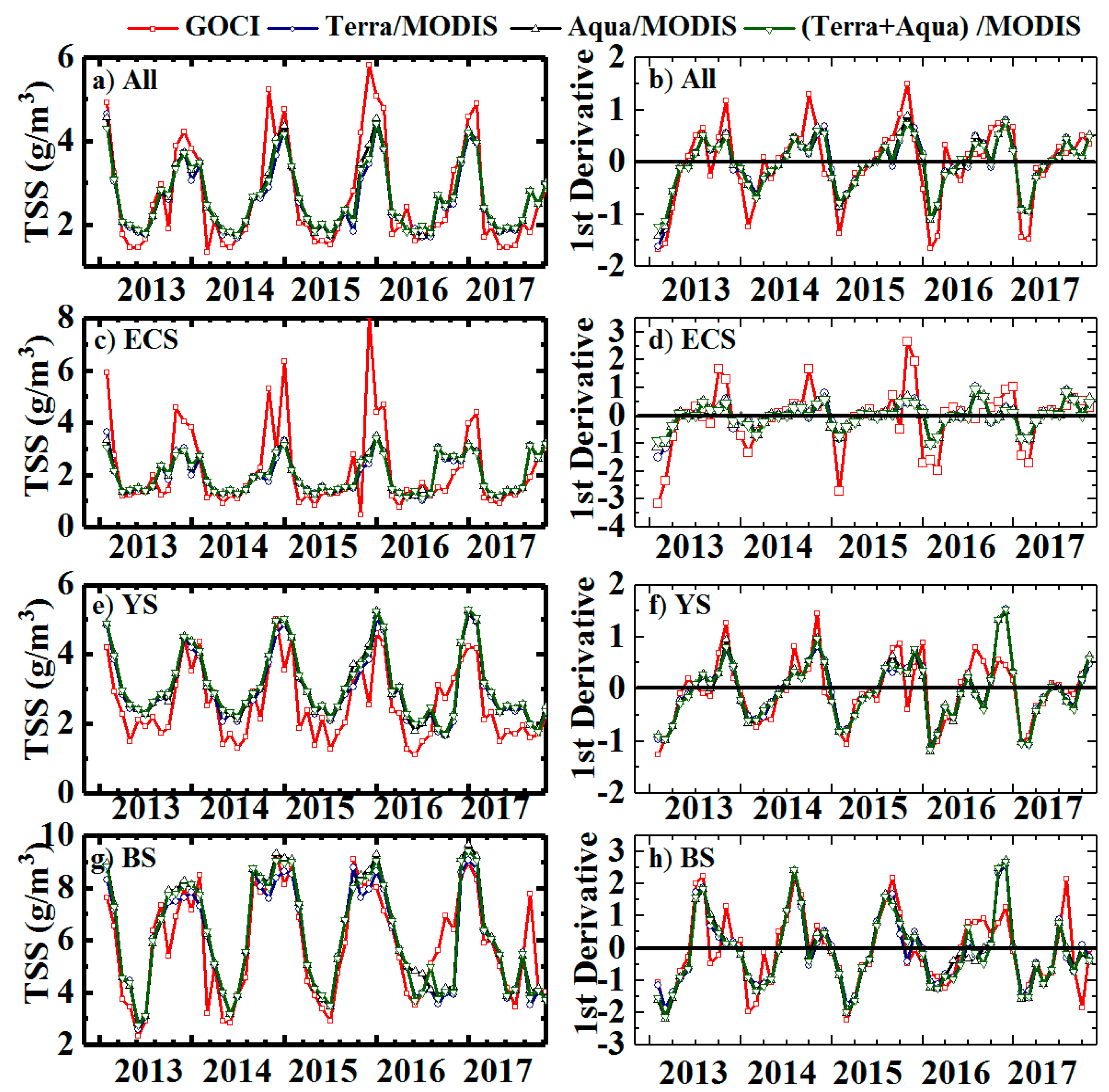
| ALL | GOCI | 1.35 | 2.07 | 5.82 | 4.47 | 4.32 | - |
| Terra | 1.69 | 2.38 | 4.65 | 2.96 | 2.76 | 8 | |
| Aqua | 1.71 | 2.41 | 4.55 | 2.84 | 2.66 | 10 | |
| Terra + Aqua | 1.77 | 2.45 | 4.42 | 2.65 | 2.80 | 10 | |
| ECS | GOCI | 0.49 | 1.42 | 8.06 | 7.57 | 16.57 | - |
| Terra | 1.00 | 1.61 | 3.65 | 2.65 | 3.65 | 13 | |
| Aqua | 1.15 | 1.64 | 3.51 | 2.35 | 3.04 | 12 | |
| Terra + Aqua | 1.10 | 1.66 | 3.42 | 2.32 | 3.71 | 11 | |
| YS | GOCI | 1.10 | 2.23 | 4.99 | 3.89 | 4.54 | - |
| Terra | 1.66 | 2.78 | 5.13 | 3.47 | 3.09 | 8 | |
| Aqua | 1.69 | 2.84 | 5.25 | 3.57 | 3.12 | 8 | |
| Terra + Aqua | 1.70 | 2.90 | 5.30 | 3.60 | 3.12 | 8 | |
| BS | GOCI | 2.32 | 5.90 | 9.23 | 6.92 | 3.99 | - |
| Terra | 2.58 | 5.86 | 9.05 | 6.47 | 3.51 | 13 | |
| Aqua | 2.80 | 5.70 | 9.66 | 6.86 | 3.45 | 10 | |
| Terra + Aqua | 2.77 | 5.80 | 9.43 | 6.65 | 3.50 | 10 |
| Bohai Sea (BS) | Yellow Sea (YS) | East China Sea (ECS) | All | |
|---|---|---|---|---|
| Terra/MODIS | 61.80% | 74.80% | 75.10% | 67.00% |
| Aqua/MODIS | 59.20% | 67.30% | 69.70% | 63.20% |
| GOCI | 32.54% | 37.28% | 47.86% | 52.24% |
| Hours of Minimum TSS Bias Errors | Hours of Minimum Cloud Coverage | |||||||
|---|---|---|---|---|---|---|---|---|
| All | ECS | BS | YS | All | ECS | BS | YS | |
| Jan | 15:30 | 15:30 | 14:30 | 15:30 | 15:30 | 15:30 | 15:30 | 15:30 |
| Feb | 13:30 | 13:30 | 14:30 | 13:30 | 15:30 | 15:30 | 15:30 | 15:30 |
| Mar | 13:30 | 13:30 | 14:30 | 13:30 | 13:30 | 13:30 | 13:30 | 13:30 |
| Apr | 14:30 | 15:30 | 14:30 | 15:30 | 11:30 | 11:30 | 13:30 | 12:30 |
| May | 14:30 | 15:30 | 12:30 | 13:30 | 14:30 | 14:30 | 14:30 | 14:30 |
| Jun | 15:30 | 15:30 | 14:30 | 14:30 | 12:30 | 11:30 | 13:30 | 12:30 |
| Jul | 15:30 | 13:30 | 15:30 | 15:30 | 12:30 | 11:30 | 13:30 | 12:30 |
| Aug | 14:30 | 14:30 | 12:30 | 15:30 | 12:30 | 11:30 | 13:30 | 13:30 |
| Sep | 13:30 | 13:30 | 12:30 | 13:30 | 12:30 | 12:30 | 13:30 | 13:30 |
| Oct | 13:30 | 13:30 | 12:30 | 13:30 | 15:30 | 15:30 | 15:30 | 15:30 |
| Nov | 15:30 | 15:30 | 15:30 | 15:30 | 13:30 | 13:30 | 13:30 | 13:30 |
| Dec | 12:30 | 15:30 | 15:30 | 15:30 | 15:30 | 15:30 | 14:30 | 15:30 |
© 2020 by the authors. Licensee MDPI, Basel, Switzerland. This article is an open access article distributed under the terms and conditions of the Creative Commons Attribution (CC BY) license (http://creativecommons.org/licenses/by/4.0/).
Share and Cite
Tian, L.; Sun, X.; Li, J.; Xing, Q.; Song, Q.; Tong, R. Sampling Uncertainties of Long-Term Remote-Sensing Suspended Sediments Monitoring over China’s Seas: Impacts of Cloud Coverage and Sediment Variations. Remote Sens. 2020, 12, 1945. https://doi.org/10.3390/rs12121945
Tian L, Sun X, Li J, Xing Q, Song Q, Tong R. Sampling Uncertainties of Long-Term Remote-Sensing Suspended Sediments Monitoring over China’s Seas: Impacts of Cloud Coverage and Sediment Variations. Remote Sensing. 2020; 12(12):1945. https://doi.org/10.3390/rs12121945
Chicago/Turabian StyleTian, Liqiao, Xianghan Sun, Jian Li, Qianguo Xing, Qingjun Song, and Ruqing Tong. 2020. "Sampling Uncertainties of Long-Term Remote-Sensing Suspended Sediments Monitoring over China’s Seas: Impacts of Cloud Coverage and Sediment Variations" Remote Sensing 12, no. 12: 1945. https://doi.org/10.3390/rs12121945
APA StyleTian, L., Sun, X., Li, J., Xing, Q., Song, Q., & Tong, R. (2020). Sampling Uncertainties of Long-Term Remote-Sensing Suspended Sediments Monitoring over China’s Seas: Impacts of Cloud Coverage and Sediment Variations. Remote Sensing, 12(12), 1945. https://doi.org/10.3390/rs12121945