Thematic Classification Accuracy Assessment with Inherently Uncertain Boundaries: An Argument for Center-Weighted Accuracy Assessment Metrics

Abstract

Accuracy assessment is one of the most important components of both applied and research-oriented remote sensing projects. For mapped classes that have sharp and easily identified boundaries, a broad array of accuracy assessment methods has been developed. However, accuracy assessment is in many cases complicated by classes that have fuzzy, indeterminate, or gradational boundaries, a condition which is common in real landscapes; for example, the boundaries of wetlands, many soil map units, and tree crowns. In such circumstances, the conventional approach of treating all reference pixels as equally important, whether located on the map close to the boundary of a class, or in the class center, can lead to misleading results. We therefore propose an accuracy assessment approach that relies on center-weighting map segment area to calculate a variety of common classification metrics including overall accuracy, class user’s and producer’s accuracy, precision, recall, specificity, and the F1 score. This method offers an augmentation of traditional assessment methods, can be used for both binary and multiclass assessment, allows for the calculation of count- and area-based measures, and permits the user to define the impact of distance from map segment edges based on a distance weighting exponent and a saturation threshold distance, after which the weighting ceases to grow. The method is demonstrated using synthetic and real examples, highlighting its use when the accuracy of maps with inherently uncertain class boundaries is evaluated.

1. Introduction

Assessment of the accuracy of maps produced through thematic classification is a central component of remote sensing, and has further applications in pattern recognition and computer vision [1,2,3,4,5,6,7]. Thematic classification is the assignment of remotely sensed data to classes within specific themes, such as land cover features [8]. Rigorous and consistent comparison of classification products, methods, and algorithms requires well-defined and appropriate metrics [4,9,10,11]. Such metrics generally assume that map features have discrete and well-defined boundaries, and that the true value of all pixels can be ascertained with equal accuracy, regardless of spatial location relative to feature edges. However, inherently uncertain boundaries are common in natural, real-world landscapes. Ignoring this uncertainty may produce a pessimistic bias in the resulting accuracy estimates [5].

Figure 1 is an example map that differentiates uplands and a variety of wetland types. The implied precision of the vector boundaries in the map is misleading: it is generally acknowledged that the delineation of wetland type boundaries has inherent uncertainty (for example, [12,13]), although the center of the map features are more consistently and reliably labeled. Uncertainty in the precise location of edges is not unique to wetland mapping; many other remote sensing applications, such as differentiating soil units (for example, [14,15,16]) and mapping individual tree crowns in forests (for example, [17,18,19,20]), face similar challenges.

Despite the fact that this uncertainty in boundary location is common in remote sensing, to our knowledge there is little guidance in the remote sensing literature on how to deal with this problem. One notable exception however, is the method developed by Brandtberg et al. [17] for fuzzy assessment of tree crown segmentation. In their work, the confidence of reference, manually interpreted tree crowns is assumed to be highest near the center of the crown and degrades towards the margins, due to the indeterminate or fuzzy nature of the crown and potential overlap with other crowns. Brandtberg et al. [17] therefore use a distance transform, calculated from the crown boundaries, to weight cells near the center of each crown higher than edge cells. By overlaying the edge-distance weighted surfaces for the predicted and associated reference crown, calculating the minimum and maximum values at each cell location, and comparing these surfaces, a summary fuzzy measure of agreement is obtained along with measures of omission, commission, and over-segmentation error [17]. Although these measures are simple to calculate, they have not been widely adopted, possibly because their relationship to traditional measures such as overall accuracy and user’s and producer’s accuracy, is not clear.

Therefore, in this paper, building upon the work of Brandtberg et al. [17], we present a general accuracy assessment approach for adjusting well-known metrics to incorporate uncertainty in the location of object or class boundaries. By applying a modification to well-known methods, our metrics are very similar to standard measures of accuracy, and thus should be easier to understand and use than would be the case with entirely new metrics.

Our proposed method is designed to:

• reduce the weight and impact of boundary areas in accuracy assessment metrics;
• support the calculation of a variety of easily interpretable and commonly used accuracy assessment metrics derived from an error matrix;
• allow the calculation of count-based and areas-based assessment metrics, as well as the estimate of population matrices;
• and be generalizable to binary, multiclass, and feature extraction accuracy assessment problems.

We illustrate our proposed approach with examples drawn from a variety of applications using synthetic and actual data that draw from tree delineation, landscape mapping with deep learning convolutional neural networks (CNNs), and geographic object based image analysis (GEOBIA) wetland mapping. However, we emphasize that center-weighting is a general method, and is potentially useful for any remote sensing application where the boundaries between classes have uncertainty.

2. Background

2.1. Standard Multiclass Remote Sensing Accuracy Assessment Metrics

Accuracy assessment of image classification and feature extract products is traditionally conducted using an error matrix (

Table 1. Example error matrix. OA = 0.84, QD = 0.06, AD = 0.10, Kappa = 0.76.

		Reference Data			UA
		A	B	C
Classification Result	A	81	9	3	0.87
	B	7	78	4	0.88
	C	12	13	93	0.79
PA		0.81	0.78	0.93

) in which classification results are compared to a finite number of validation samples representing mapping or assessment units, such as pixels, blocks of a defined size, or image objects. The validation data are generally assumed to be correct and to represent the “ground truth.” By cross tabulating the classification product and associated validation samples, a variety of metrics can be calculated, including overall accuracy (OA, Equation (1)), class-level accuracies as producer’s accuracy (PA) (1–omission error) and user’s accuracy (UA) (1–commission error) (Equations (2) and (3)), and the Kappa statistic (Equation (4)) [1,2,3,4,7,21]. Additional measures have also been proposed that make use of this framework. For examples, Pontius and Millones [22], who advocate against the use of Kappa, introduced the alternative measures of quantity and allocation disagreement. Quantity disagreement (QD) is the disagreement between the classification and reference data resulting from a difference in proportion of classes while allocation disagreement (AD) assesses a difference in the spatial location of classes, and the two measures sum to overall error (1–OA).

$$\mathrm{Overall}\mathrm{Accuracy}(\mathrm{OA})=\frac{Number of Correctly Classified Samples}{Number of Total Samples}$$

(1)

$$\mathrm{Class}\mathrm{Producer}\text{’}\mathrm{s}\mathrm{Accuracy}(\mathrm{PA})=\frac{Number of Correctly Classified Samples in Category}{Number of Samples from Reference Data in Category}$$

(2)

$$\mathrm{Class}\mathrm{User}\text{’}\mathrm{s}\mathrm{Accuracy}(\mathrm{UA})=\frac{Number of Correctly Classified Samples in Category}{Number of Samples Classified to that Category}$$

(3)

$$\mathrm{Kappa}\mathrm{Statistic}=\frac{Overall Accuracy-Estimated Chance Agreement}{1-Estimated Chance Agreement}$$

(4)

2.2. Accuracy Assesement of Binary Classifications

When only a single class is differentiated from the image background, as is common in feature extraction tasks, or when only two classes are mapped to generate a binary output, an alternative terminology is commonly used. Specifically, if one category represents a positive case while the other represents a background or negative case, the terms true positive (TP), false positive (FP), true negative (TN), and false negative (FN) are used. TP samples are those that are in the positive class and are correctly mapped as positive while FPs are not in the positive class but are incorrectly mapped as positive. TNs are correctly mapped as negative while FNs are mapped as negative when they are actually positive (

Table 2. Example binary confusion matrix and associated terminology.

		Reference Data
		True	False
Classification Result	True	TP	FP
	False	FN	TN

). From this cross tabulation, it is possible to derive a variety of metrics. Precision (Equation (5)) represents the proportion of the samples that is correctly classified within the samples predicted to be positive, and is equivalent to user’s accuracy (1–commission error) for the positive class. Recall or sensitivity (Equation (6)) represents the proportion of the reference data for the positive class that is correctly classified, and is equivalent to producer’s accuracy (1–omission error) for that class. The F1 score (Equation (8)) is the harmonic mean of precision and recall, while specificity (Equation (7)) represents the proportion of negative reference samples that is correctly predicted, and is thus equivalent to the producer’s accuracy for the negative class [23].

$$\mathrm{Precision}=\frac{TP}{TP+FP}$$

(5)

$$\mathrm{Recall}\mathrm{or}\mathrm{Sensitivity}=\frac{TP}{TP+FN}$$

(6)

$$\mathrm{Specificity}=\frac{TN}{TN+FP}$$

(7)

$$\mathrm{F}1\mathrm{Score}=\frac{2\times Precision\times Recall}{Precision+Recall}$$

(8)

The computer vision, feature recognition, and deep learning research communities often calculate additional binary measures by comparing each validation feature to its predicted extent in the image based on overlapping bounding boxes or feature masks. For example, the intersection-over-union (IoU), or Jaccard Index, which is described in Equation (9) and illustrated in Figure 2, is the proportion that is shared of the combined area of the reference bounding box and predicted bounding box, or the area of intersection divided by the area of union of the two objects. Correct or incorrect predictions can be defined based on a minimum IoU measure that is deemed acceptable, for example, by using an IoU threshold of 0.5 or by averaging over a range of different thresholds. In order to generate a single performance metric from multiple features, predictions can be ranked based on the prediction confidence. From these ranked data, a precision–recall curve can be generated and average precision (AP) can be approximated by estimating the area under this curve. The metric obtained when AP is averaged for multiple categories or classes is commonly called mean average precision (mAP) [24].

$$\mathrm{IoU}=\frac{Area of Intersection}{Area of Union}$$

(9)

2.3. GEOBIA Accuracy Asssessment

GEOBIA classifications, in which the input image is first divided into homogenous regions or segments, and then classified using the segments as the spatial units, is particularly complex. It is generally advised to assess both the thematic accuracy and the quality of the segmentation, though in practice this recommendation is rarely fully implemented [3,25,26]. This can be partially attributed to the challenging nature of, lack of standardization in, and variety of options proposed for segmentation assessment, as highlighted by the available literature on this topic [26,27,28,29,30,31,32,33,34,35,36,37]. In a recent review of segmentation assessment methods, Chen et al. [31] provide a categorization of the wide range of available assessment metrics, including subjective methods that are based on visual assessment and the evaluator’s best judgment and empirical methods that rely on quantitative evaluation in the form of assessment metrics. Costa et al. [32] provide a summary of supervised segmentation evaluation metrics and catalog 66 measures that offer a quantitative evaluation of geometric correspondence between segments and reference data concerning area, position, or both. Yang et al. [34] offer a review of a variety of unsupervised methods that rely on assessing intra-region uniformity, inter-region disparity, object shape, or a combination of considerations. It is common for studies to recommend a set of measures that quantify different components of segmentation quality. For example, Lizarazo [28] introduced the STEP method which relies on supervised assessment and requires the calculation of shape, theme, edge, and position similarity measures.

Despite the many GEOBIA accuracy assessment methods, there are few approaches that formalize uncertainty in boundary edges. Most segmentation metrics assume that the reference data are correct and that there is no ambiguity in feature boundaries or edges. One approach takes a more nuanced view by conceptualizing the segments and reference data as separate representations, with an evaluation performed to assess how well the segments correspond to the manual interpretation [27], a characteristic that Clinton et al. [27] describe as “goodness.” A notable example of a study that expressly considers uncertainty in edges is that of Unnikrishnan et al. [33], who proposed the normalized probabilistic Rand (NPR) index. This index compares a segmentation result to a set of reference features, such as manually digitized features produced by multiple analysts, thereby incorporating boundary ambiguity.

2.4. Accuracy Assessment and Pessimisitc Bias

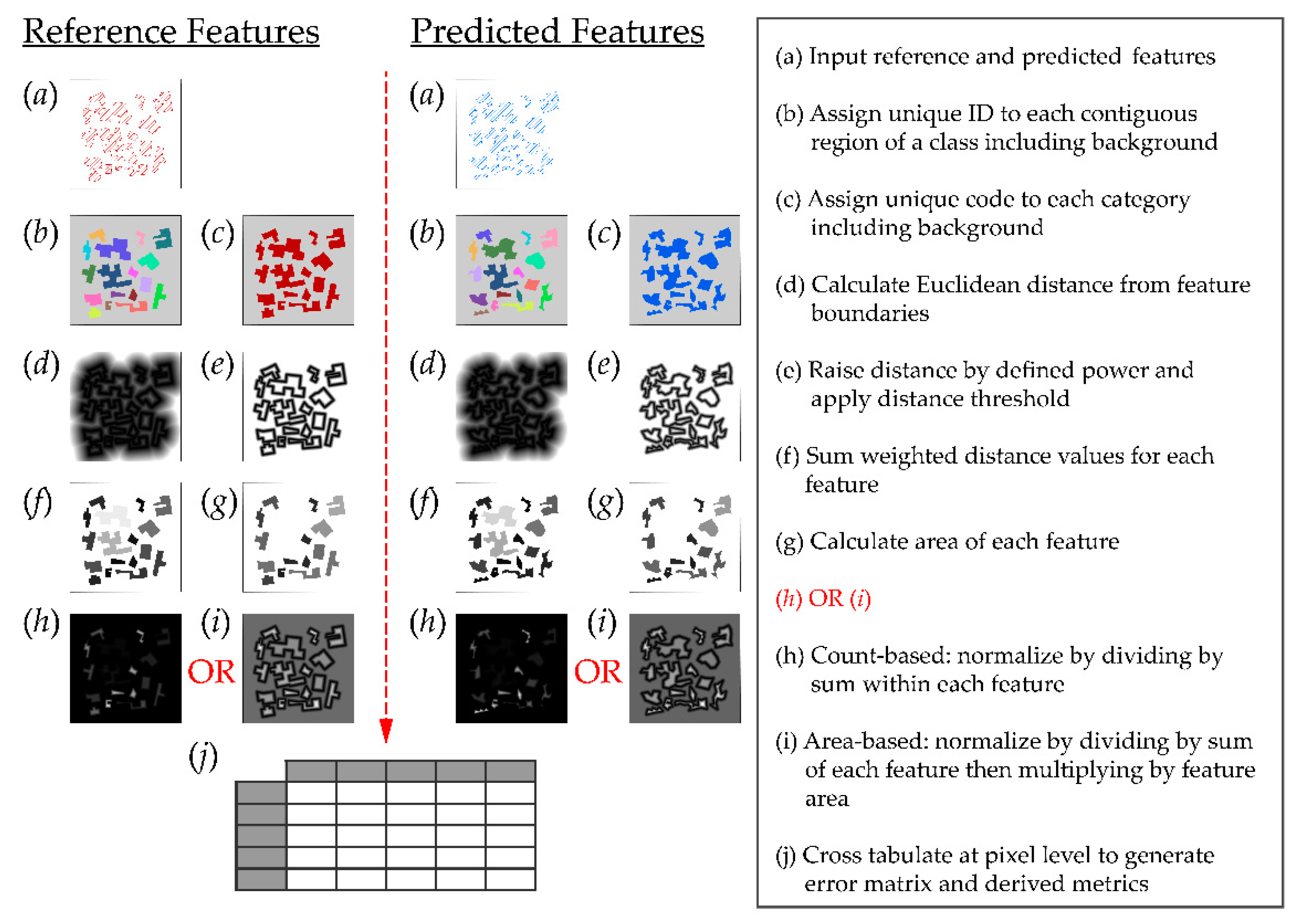
Foody [5] suggests that thematic accuracy assessment methods used in remote sensing can be overly harsh, especially in comparison to methods used by other disciplines in which thematic map generation is a common task. For example, unit boundaries on geologic maps are not commonly assessed with the same level of site-specific rigor as land cover maps, which can be partially attributed to the difficulty of accurately defining and validating these map units and also mapping standards and traditions within the discipline [5]. Harshness in image classification accuracy assessment can be attributed to reliance on site-specific measures as represented by the error matrix and its derivatives, which generally assume that all disagreements between the reference data and the evaluated map result from errors in the map. Furthermore, analysis of the error matrix generally assumes the location of the reference samples is irrelevant, and indeed some variant of random sampling is required for statistical inference. However, errors can arise from many sources, including difficulty of defining discrete categories and associated boundaries, mixed pixels, spatial reference and misalignment issues, and uncertainty or error in the validation data, which are generally assumed to represent the “ground truth” despite this uncertainty [5].

Some methods have been suggested to potentially reduce this pessimistic bias. For example, to minimize the impact of misalignment, it has been suggested to use the majority class within 3 × 3 cell windows, rather than individual pixels [38,39]. Error is generally more prominent near thematic boundaries; thus, avoiding selecting validation features near boundaries has been shown to reduce the reported classification error [5,40]. For example, Fuller et al. [40] reported a 25% to 71% increase in accuracy when excluding boundary regions from an assessment. Nevertheless, simply excluding boundary pixels entirely undermines the ideal of a random sample, and begs the question of what to do if the boundary regions are more than one pixel wide.

3. Methods

The map segment center-weighted accuracy assessment metric is conceptualized in Figure 3 for synthetic data representing a feature extraction problem where each shape is an instance of the same class against a background. For simulation purposes, the synthetic data are generated as vector data, and then rasterized as described below. In application of the approach to real data, rasterization is not generally needed, unless the reference data are in vector format. In Figure 3, the first step is that each spatially contiguous area of a class in the reference and predicted data (Figure 3a) is defined as a unique instance of that class, and two raster grids for both the reference and predicted data are produced at a user-defined cell size to represent the segments’ unique identifiers and class codes (Figure 3b,c). If the data are not spatially contiguous, then unmapped areas are assigned to a background class. Next, Euclidean distance from map segment boundaries is calculated relative to the projected coordinate system of the data, which results in raster images of the distance from boundaries to each cell in the validation and classification maps, respectively (Figure 3d).

The default is for the weightings to increase progressively, so that the largest weight is at the center of the polygon, defined as the point farthest from any edge. However, it may be appropriate to stop increasing the weights at a specified distance from the edge. For example, an analyst might know that the uncertainty in the estimation of the boundary of the reference segment is 5 m. Therefore, as an option, the user can set the saturation threshold distance, and all cells with Euclidean distance values greater than this distance are recoded to the weighting at the threshold distance.

In order to specify the mathematical model of how values increase with distance, a power or exponent is then applied to the distance values, where larger powers increase the relative influence or weight of center cells (Figure 3e). For example, with an exponent of 1.0, the weightings increase linearly with distance from the edge, but with an exponent greater than 1.0, the weightings grow increasingly rapidly as the distance from the edge increases. An exponent less than 1.0 also results in an increase in weightings with distance, but the increases get progressively smaller with distance from the edge. An exponent of 0 is equivalent to traditional accuracy assessment, with no differential weighting based on distance. In summary, the weighting D_x applied to pixel x is calculated from:

$$D_x=distance{(x,b)}^E$$

(10)

where b is the closest boundary pixel, distance() is a distance function, specifying the number of pixels between x and b, and E is the user-specified exponent.

Normalization is then performed relative to either map segment counts or segment areas. Normalization using segment counts is appropriate if the accuracy assessment focuses on the number of objects, for example, the number of trees. On the other hand, if area covered by the mapped classes or the size of map segments is of interest, then area-based normalization should be chosen.

For map segment count normalization, each cell value within a particular segment is divided by the total weights for all cells within that map segment (Figure 3f), so that each individual segment sums to 1, and the sum of the cells within the map is equivalent to the number of mapped segments, including the background class (Figure 3h). Thus, the weight W_x^Count of a cell at pixel x is calculated from:

$$W_x^{\mathrm{Count}}=\frac{D_x}{{{\displaystyle \sum }}_{i=1}^{i=n}{D}_i}$$

(11)

where n is the number of pixels in the segment of interest and i represents a location within that segment.

In order to normalize relative to area, each cell is first divided by the sum of the weights of the cells constituting the segment within which it occurs, and then multiplied by the area of that segment (Figure 3g). The sum of the resulting normalized weights for each map segment is equivalent to the segment area, and the total sum over the map represents the area of the map (Figure 3i). The resulting equation is:

$$W_x^{\mathrm{Area}}=D_x\times \frac{n}{{{\displaystyle \sum }}_{i=1}^{i=n}{D}_i}$$

(12)

In order to generate a confusion matrix from the raster surfaces (Figure 3j), the reference and predicted results, as described above, are summed at each cell location and then divided by two. Thus the summary statistics incorporate a weighting of distance to both the reference segment edges and the predicted segment edges. These summary values are then cross-tabulated using the reference and predicted class codes at each cell. If a count-based method is used, then all cells in the matrix will sum to the average number of segments mapped in the reference and predicted datasets. If an area-based method is used, then the error matrix will sum to the total area of the mapped extent.

Following the tabulation of the error matrix, derived measures can be calculated. For a multiclass problem, this includes OA and class user’s and producer’s accuracy. It is also possible to calculate the Kappa statistic or the alternative AD and QD measures. For a binary or feature extraction problem, precision, recall, specificity, and the F1 score are calculated relative to the positive class. Thus, common assessment metrics are generated in which the center areas of map segments have a larger contribution than near-edge locations.

This process is implemented in the free and open-source data analysis software R [41]. We rely on the raster package [42] for handling raster data; the sf package [43] for processing vector data; the dplyr package for basic data manipulation [44]; and the caret [45], diffeR [46], and rfUtilities [47] packages for calculation of accuracy assessment metrics. In order to speed up the generation and processing of raster data, we also use the recently released fasterize [48] and fasterRaster [49] packages made available through GitHub. The code is provided as an R function with associated documentation in the Supplementary Materials for this paper. Although we use R in this implementation, other platforms could be used to perform this validation process, such as ArcGIS and ArcPy [50] or QGIS [51] and additional open-source Python libraries [52].

4. Demonstrations and Metric Characteristics

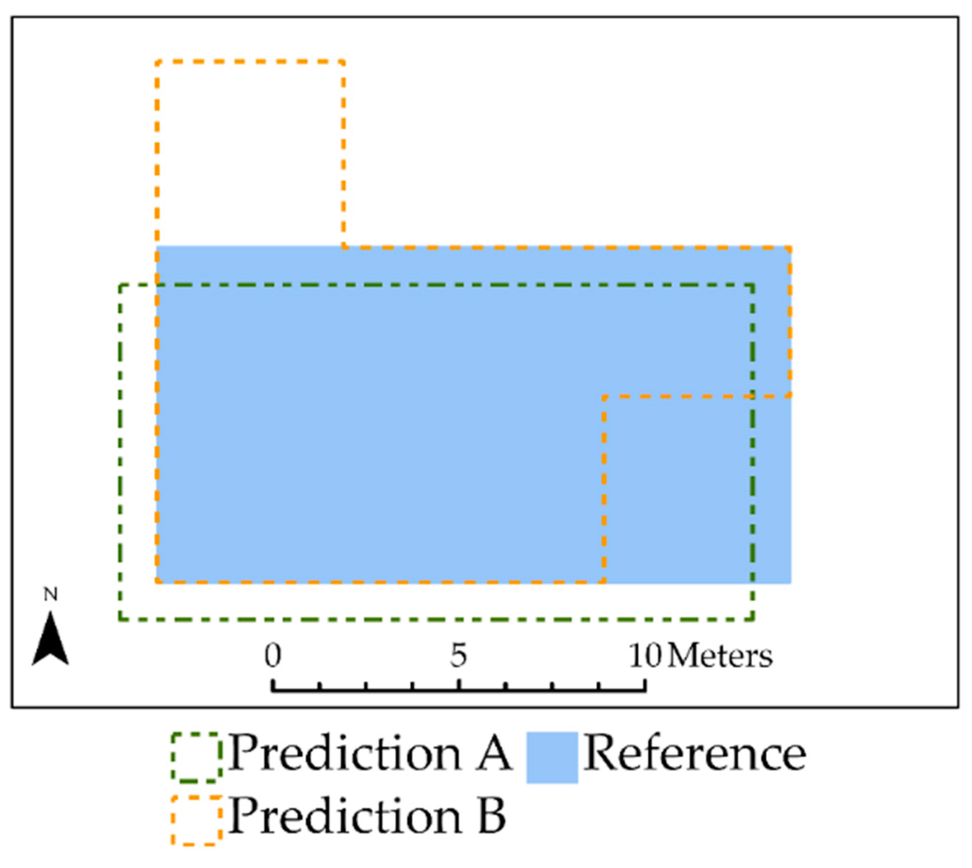
4.1. Example 1: Limitations of Standard Area-Based Accuracy Assessment Compared to Center Weighting

In this first example, synthetic data are used to illustrate the information that is lost by failing to consider the location of error, and thus how traditional, area-based accuracy assessment fails to distinguish important differences between classifications (Figure 4). Two results, Prediction A and Prediction B, are compared to a reference feature. They both have the same percentage overlap or shared area with the reference feature, and thus have identical traditional accuracy measures, as represented by the rows with a distance weighting exponent of 0 in

Table 3. Comparison of validation results for the synthetic features shown in Figure 4.

Prediction	Distance Weighting Exponent	Distance Threshold	Precision	Recall	Specificity	F1 Score
A	0	NA	0.837	0.837	0.922	0.837
B	0	NA	0.837	0.837	0.922	0.837
A	1	10 m	0.963	0.965	0.983	0.964
B	1	10 m	0.871	0.876	0.938	0.873

. However, it is visually clear from Figure 4 that Prediction A conforms more closely than B to the reference feature, based on shape and overlap of the center areas. The IoU measure would also indicate that Prediction A is more accurate, since a larger proportion of the union of the bounding boxes for Prediction A and the reference feature is shared in comparison to Prediction B and the reference feature. However, boundary uncertainty is not inherently incorporated in IoU and thus that measure is not an appropriate general measure for remote sensing accuracy assessment.

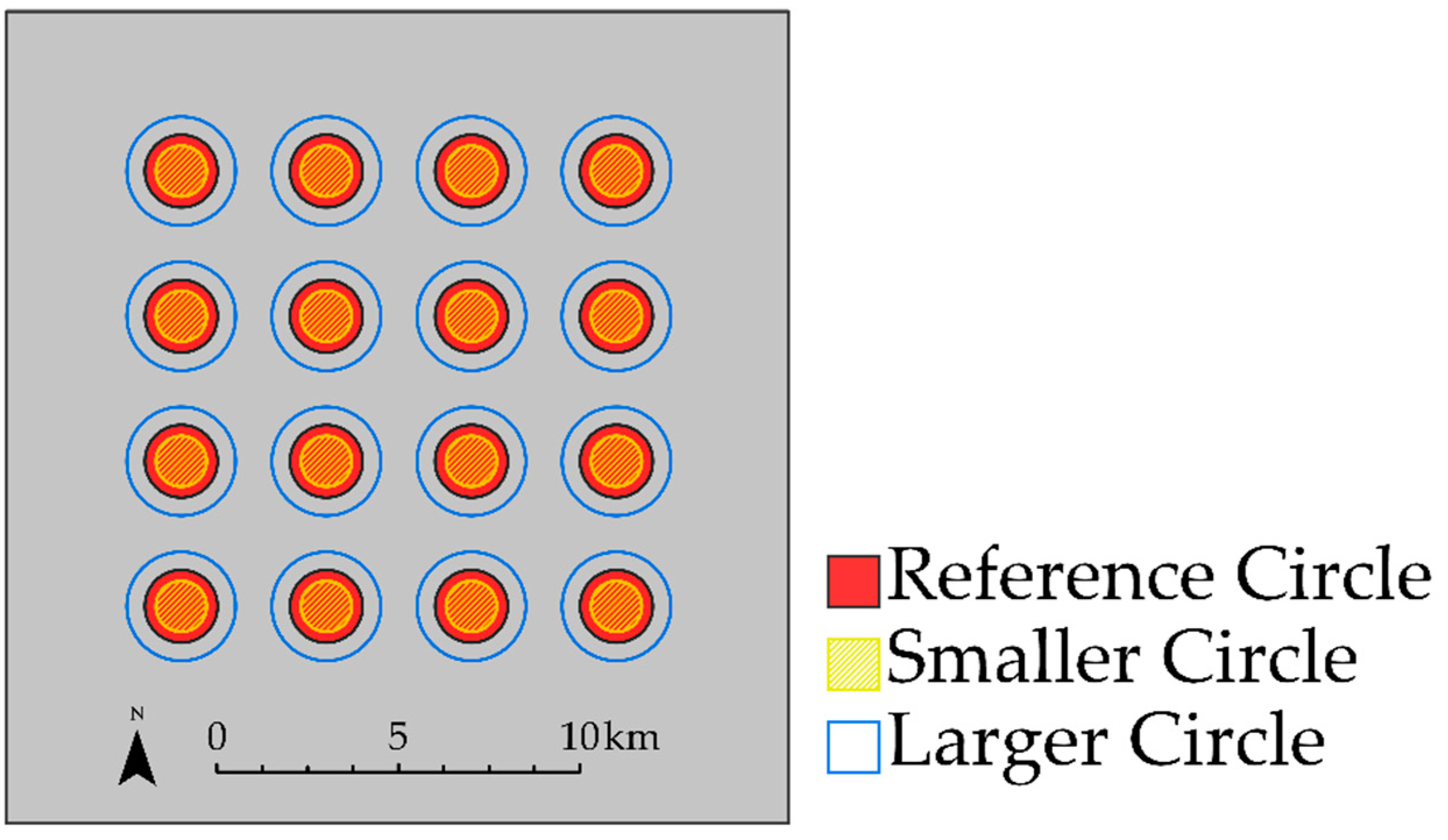
4.2. Example 2: Impact of Over- and Under-Predicting Feature Area

When the distance weighting exponent is set to 1 (i.e., center-weighting) and the saturation threshold distance is set to a sufficiently high value that the weighting increases to the center of the object (e.g., a value of 10 m), the accuracy measures for both Predictions A and B are higher than the values using the traditional approach (Table 3), because in both classifications the error tends to be concentrated towards the edges of the object. However, with center-weighting the accuracy values are much higher for A than B (e.g., an F1 score of 0.964 vs. 0.873), thus clearly differentiating the performance of the two classifications, and providing an objective measure of the improvement of A compared to B.

In this second example, we demonstrate the impact of over- and under-predicting map segment area using a set of synthetic data (Figure 5). The reference segments for the positive class are red circles, with a uniform radius. Two predictions are overlaid on the map. The first prediction results in larger circles (i.e., an over-prediction of the reference class), shown with blue outlines in Figure 5. The second prediction results in smaller circles (and thus an under-prediction), shown with a yellow hash pattern. For simplicity, the centers of the predicted circles are kept at the same location as the reference circles. We use an area-based accuracy assessment method, a distance saturation threshold of 500 m, and vary the distance weighting to explore changes in the resulting metrics.

Table 4. Comparison of metrics generated using different distance weighting exponents. The “larger” classification scenario corresponds to the blue outlines in Figure 4; the “smaller” scenario corresponds to the circles shown using the yellow hash pattern. A distance weighting exponent of 0.0 represents the traditional (unweighted) method.

Size of Classified Feature Relative to Reference Data	Distance Weighting Exponent	Precision	Recall
Larger	0.0	0.445	1.000
Larger	0.5	0.542	1.000
Larger	1.0	0.611	1.000
Larger	1.5	0.663	1.000
Larger	2.0	0.703	1.000
Larger	2.5	0.735	1.000
Larger	3.0	0.761	1.000
Smaller	0.0	1.000	0.490
Smaller	0.5	1.000	0.642
Smaller	1.0	1.000	0.750
Smaller	1.5	1.000	0.826
Smaller	2.0	1.000	0.878
Smaller	2.5	1.000	0.914
Smaller	3.0	1.000	0.939

shows the results of this experiment. When over-predicting positive map segment area (the classification shown with the blue outline), recall is always 1, no matter the distance weighting used, since there is no false negative or omission error. In contrast, systematically under-estimating positive segment area results in a precision of 1 since there is no false positive or commission error. By varying the distance weighting exponent values from 0 to 3, we observe steady increases in either precision or recall, which is expected since the features are not translated or offset and share the same center.

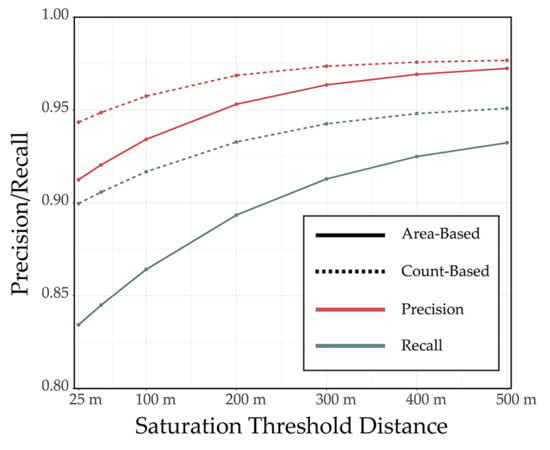
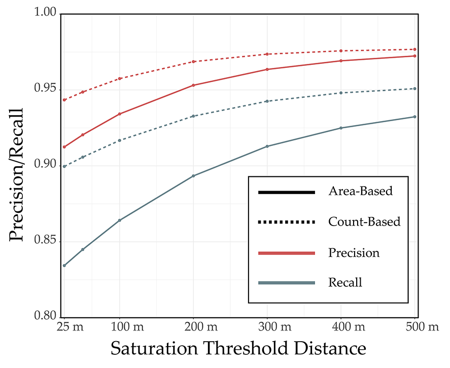
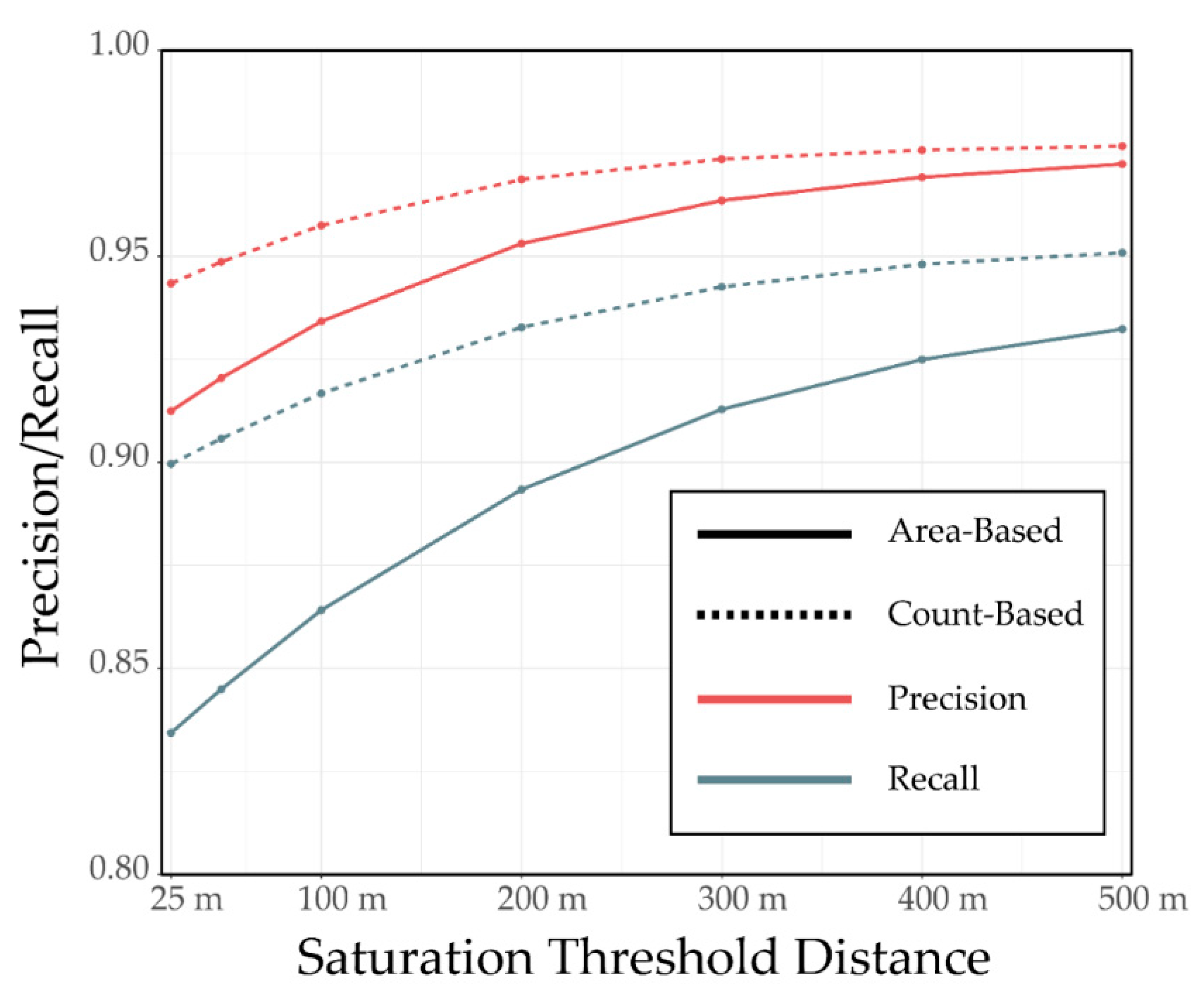
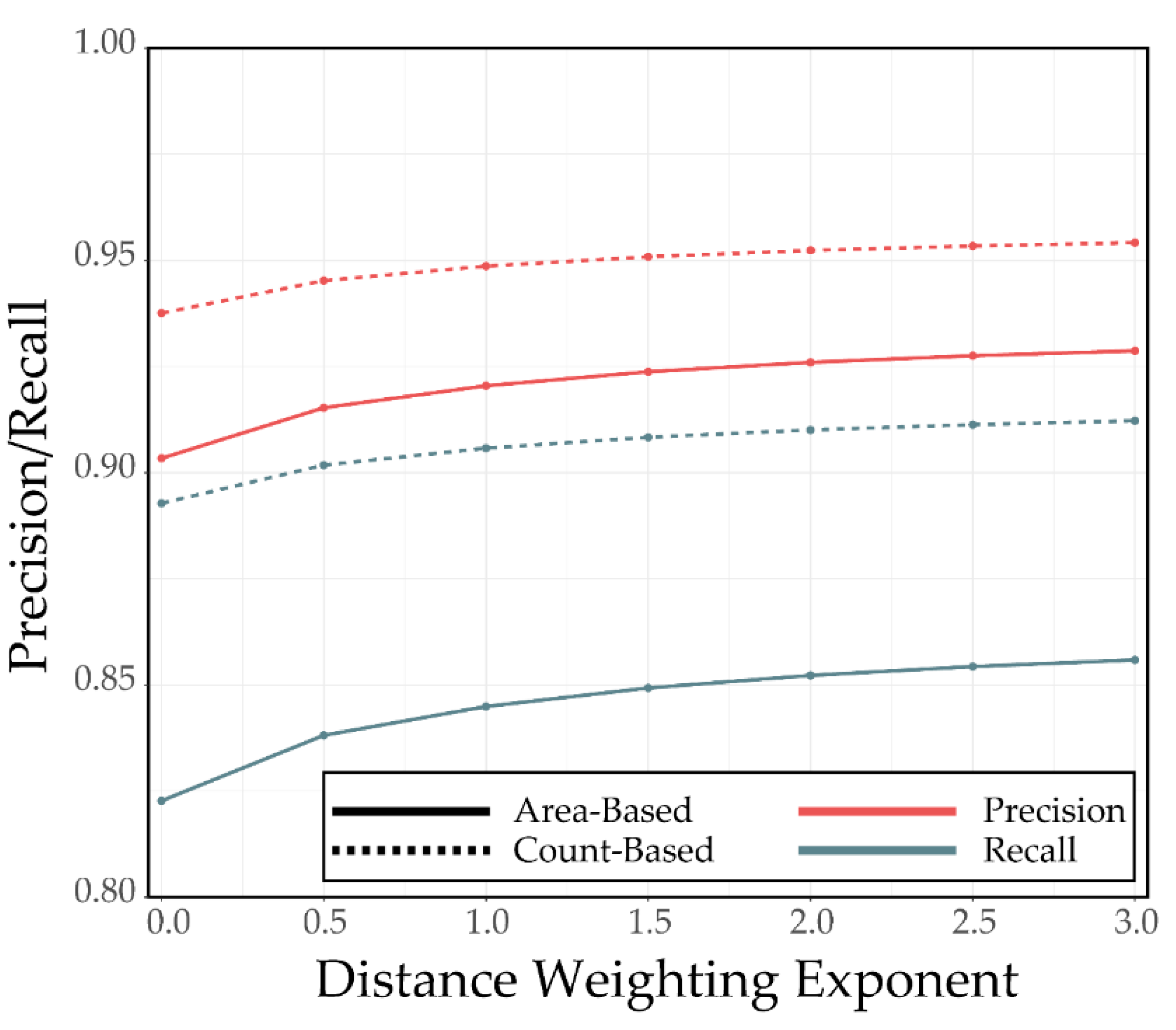
4.3. Example 3: Impact of Distance Weighting Exponent and Saturation Distance for Synthetic Features

Figure 6 shows another set of synthetic reference and validation data representing a single-class feature extraction problem, which is used to demonstrate the impact of varying the saturation distance threshold and distance weighting exponent. Results were generated using both the count-based and area-based methods. Figure 7 shows the results when the saturation distance threshold is varied from 25 to 500 m and the weighting is held constant at 1. As the saturation distance threshold increases, the resulting precision and recall estimates also increase as the center of the map segments are attributed more relative weight in the calculations. This is expected since the reference and predicted data generally overlap and difference is concentrated at the segment margins.

Figure 8 shows the results when holding the saturation distance constant at 50 m while varying the distance weighting exponent from 0 to 3. As the distance weighting exponent increases, the resulting precision and recall also increase as edges are assigned a smaller relative weight in the calculations.

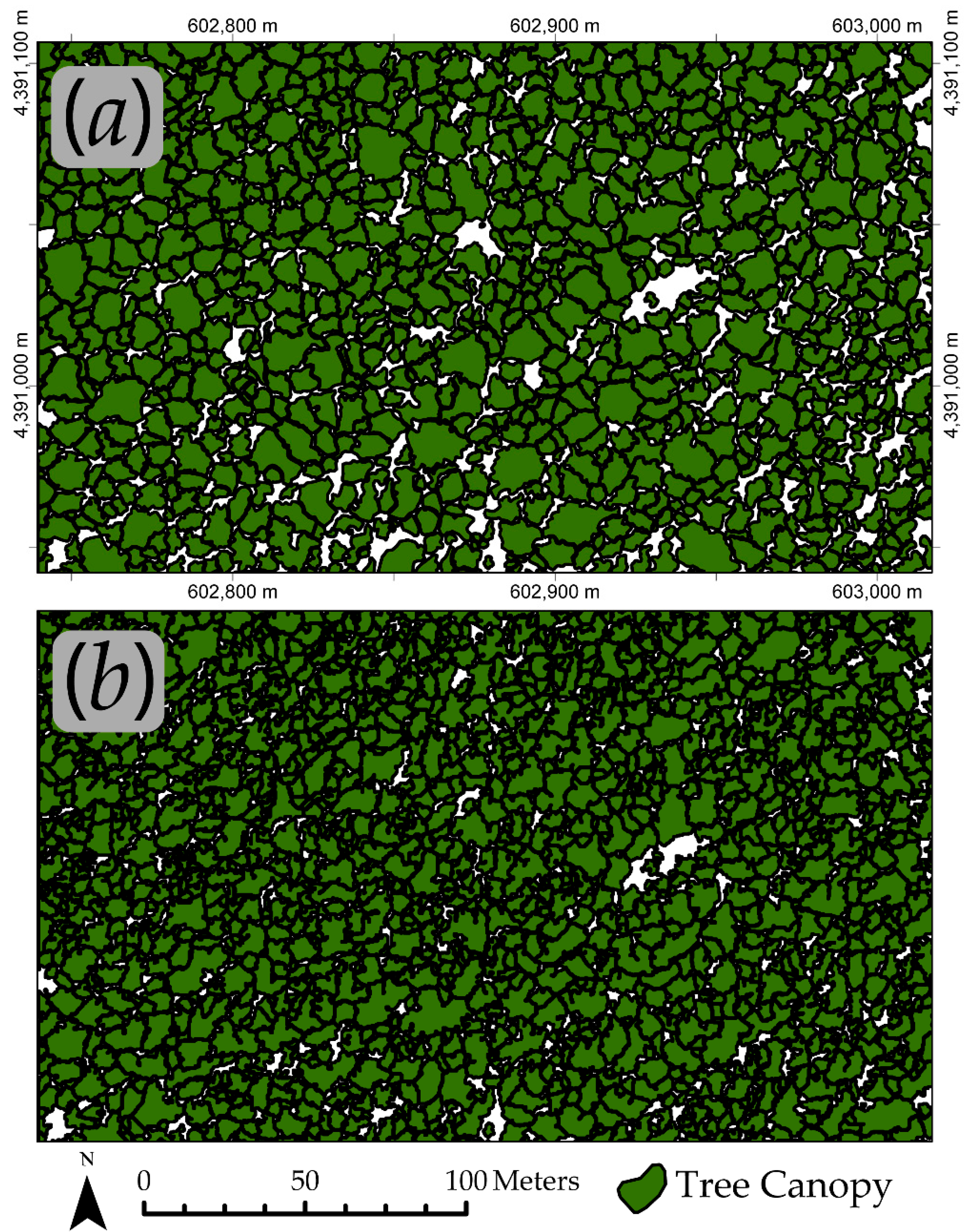
4.4. Example 4: Individual Tree Crown Delineation

The data shown in Figure 9 are from a study by Warner et al. [53] and relate to the mapping of individual tree crowns in a deciduous forest stand. Manually delineated tree crowns (Figure 9a) are used as reference data and compared to crowns generated using a minimum cost path algorithm (Figure 9b). As there is inherent uncertainty in delineating tree crown boundaries, this is a good example of where the proposed center-weighted method would be useful. Comparisons are made using both the area-based and count-based methods and with distance weighting exponents of 0 and 1. When using a distance weighting of 1, a saturation distance threshold of 5 m is applied.

The results are summarized in

Table 5. Results for individual tree crown delineation.

Method	Distance Weighting Exponent	Distance Threshold	Precision	Recall	Specificity	F1 Score
Area-Based	0	NA	0.872	0.912	0.590	0.892
Area-Based	1	5 m	0.925	0.949	0.758	0.937
Count-Based	0	NA	0.883	0.969	NA	0.924
Count-Based	1	5 m	0.928	0.980	NA	0.945

. Center-weighting with a distance weighting exponent of 1 results in higher assessment metrics in comparison to an exponent of 0, or traditional accuracy assessment, which indicates that disagreement is concentrated near feature boundaries. Because these boundaries were manually delineated and are thus inherently uncertain, the less harsh assessment of the predicted tree crown extents is more appropriate than the traditional assessment, which assumes the reference data are without error.

For the count-based method, specificity, which focuses on the true negatives and false positives (Equation (7)), is not reported in Table 5. This is because canopy gaps, the negative or background class in this example, are interconnected, resulting in a single count, making an evaluation of the number of true negatives not very useful. However, if the negative class were segmented in a manner similar to that of the positive class, then specificity for count-based metrics may be of value.

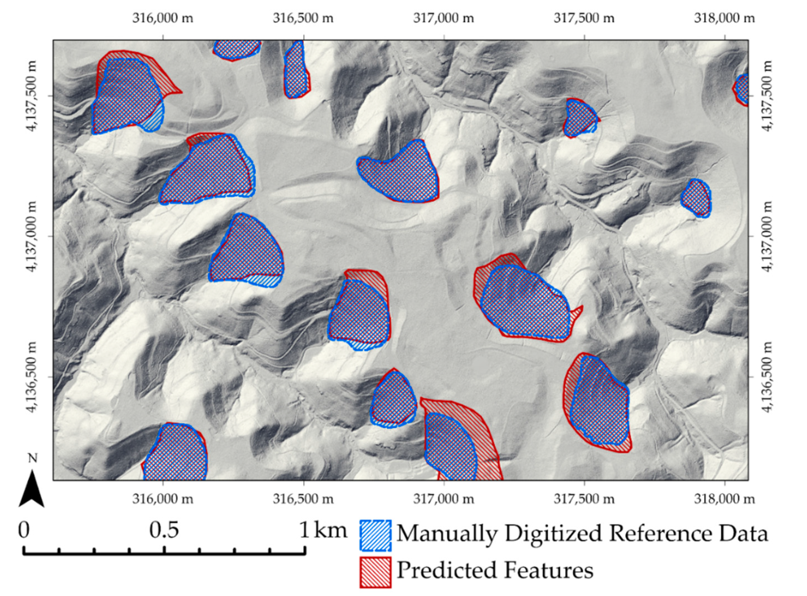
4.5. Example 5: Results for Assessment of Valley Fill Face Extraction

This example relates to a feature extraction problem where a single class is differentiated from the background. The data used are a subset of the map segments used in our prior publication in which we mapped valley fill faces from digital terrain data using convolutional neural networks (CNN)-based deep learning [54]. Figure 10 shows a subset of the data. The manually digitized reference data are shown in blue while the extents predicted using deep learning are shown in red. This experiment uses both the count-based and area-based methods, distance weightings of 0 and 1, and a processing cell size of 5 m.

When a distance weighting of 0 is applied, or a standard accuracy assessment is used, recall is calculated as 0.888, precision as 0.778, specificity as 0.996, and the F1 score as 0.829 (

Table 6. Assessment results for extraction of valley fill faces using deep learning.

Method	Distance Weight	Distance Threshold	Precision	Recall	Specificity	F1 Score
Area-Based	0	50 m	0.888	0.778	0.996	0.829
Area-Based	1	50 m	0.943	0.824	0.998	0.880
Count-Based	0	50 m	0.919	0.844	NA	0.880
Count-Based	1	50 m	0.957	0.874	NA	0.913

). When increasing the weighting to 1 to apply a linear distance weighting, all measures increase since the features commonly share interior area and differ at the fuzzy boundaries. A similar pattern is observed for the count-based method. As with the tree crown data, the specificity results for the count-based method is not reported because there is only a single background segment.

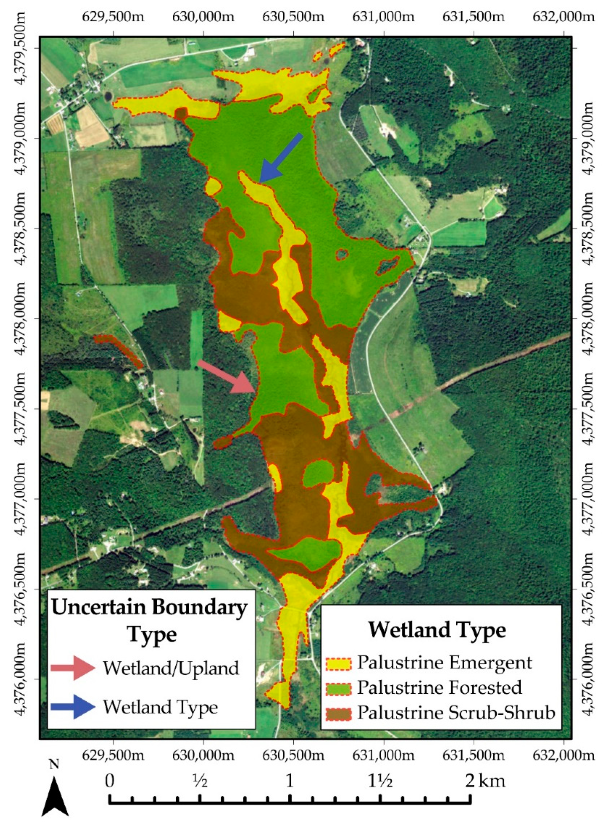
4.6. Example 6: Multiclass and Spatially Contiguous Classification Assessment

Lastly, we will now explore a multiclass assessment. The data used in this example and shown in Figure 11 relate to the classification of types of palustrine wetlands (palustrine emergent (PSS), palustrine forested (PFO), and palustrine scrub–shrub (PSS)) and the differentiation of wetlands from upland areas. The data analyzed cover the full extent of Crawford County, Pennsylvania, in the United States. Two different representations of palustrine wetlands are compared: data from the National Wetland Inventory (NWI) [55] and more recently generated boundaries provided by the University of Vermont (UVM) Spatial Analysis Laboratory (SAL) [56]. Neither of these datasets is without uncertainty. This is typical of many remote sensing studies that rely on reference data from photointerpretation or other sources of information that are in many cases not the product of exhaustive ground-checking. In wetland studies, often the reference data come from a regional or national database [13]. In GEOBIA studies, this problem of spatial uncertainty is compounded because it is usually not feasible to produce field-based polygon boundaries for the accuracy assessment [57].

For the sake of demonstration, we treat the more recently produced SAL data as reference data, and the NWI data as predictions. This experiment was conducted using distance weighting exponents of 0 (i.e., conventional accuracy assessment) and 1 (linear distance weighting), and the area-based method. For both experiments, the distance saturation threshold was set to 50 m, which was selected based on the size distribution of the wetlands in the county, and processing was conducted using 10 m spatial resolution raster grids.

As highlighted by the resulting error matrices (

Table 7. Results for multiclass classification with a distance weighting index of 0 (equivalent to traditional accuracy assessment, with uniform weighting of all pixels). OA = 0.824, Kappa = 0.297, AD = 0.046, QD = 0.130.

		Reference Data				UA
		Upland	PEM	PFO	PSS
Classification Result	Upland	2,104,233,840	37,569,359	330,286,054	22,279,483	0.981
	PEM	8,071,915	13,511,700	2,841,000	4,792,900	0.202
	PFO	24,834,561	5,494,000	84,684,200	5,852,100	0.197
	PSS	8,715,288	10,262,200	12,249,500	10,587,500	0.243
PA		0.844	0.462	0.701	0.253

PEM = palustrine emergent, PFO = palustrine forested, PSS = palustrine scrub–shrub.

and

Table 8. Results for multiclass classification with a distance weighting index of 1 (equivalent to a linear increase in with distance from the edge). OA = 0.836, Kappa = 0.330, AD = 0.038, QD = 0.126.

		Reference Data				UA
		Upland	PEM	PFO	PSS
Classification Result	Upland	2,127,035,350	34,638,122	314,708,326	20,108,600	0.986
	PEM	6,653,671	14,487,761	1,801,477	4,969,928	0.223
	PFO	17,879,632	5,098,774	91,415,185	5,513,237	0.218
	PSS	6,613,750	10,722,481	10,877,585	11,237,370	0.269
PA		0.852	0.519	0.762	0.285

) and associated assessment metrics, wetlands and uplands were generally well separated, but there was significant confusion between the different palustrine wetland classes. When applying the linear feature center-weighted method, OA, Kappa, and all class user’s and producer’s accuracies increased, and the AD and QD (which measure error rather than accuracy) decreased compared to the traditional approach, indicating that some, but not all, of the disagreement is on the edges of the classes. The PEM producer’s accuracy changed the largest amount (from 0.46 to 0.52), which is consistent with the observation that PEM in Figure 9a,b is generally more similar between the two data sets than the other classes, and that error is more concentrated on edges. Notably, the QD disagreement magnitude is much greater than the AD in the accuracy assessments, which implies that most of the differences in the maps is due to differences in the proportions of the classes. However, the AD changed much more than the QD with distance weighting compared to the traditional approach, reinforcing the interpretation that the conventional accuracy assessment is penalizing small differences in the boundaries.

5. Discussion

When boundaries are inherently uncertain, accuracy assessment metrics that assume sharp, discrete boundaries can be misleading, overlay harsh, and introduce pessimistic bias into the assessment and the perceived quality of the map product. Uncertainty in boundary location can be caused by the imposition of an arbitrary pixel size on the landscape. However, in many cases, the boundaries in the landscape themselves are inherently fuzzy, indeterminate, or gradational. In such circumstances, it can be useful to adopt assessment techniques that weight the center areas of reference and predicted map segments higher than the edges. Here, we demonstrated a method that accomplishes this center-weighting and argue that it is a useful assessment metric when mapping map segments with inherently indeterminate boundaries, which is not uncommon in natural, real-world landscapes. This applies not only to objects with boundaries that are in many cases inherently fuzzy, such as wetlands, but also to landscape features such as valley fill faces. Based on the experimental results and demonstrations provided here, we argue that this method has many favorable attributes, including its applicability to both multiclass mapping and single-class feature extraction problems, and its consistency, which is not affected by translation or rotation direction. The proposed method allows for the calculation of a variety of common assessment metrics derived from an error matrix. The method is thus a modification of standard approaches, rather than an entirely new method. This is an important benefit of this approach, as it aids in its interpretability.

Another strength of the method is that it allows for the calculation of both area-based and count-based metrics. Area-based metrics are directly analogous to conventional accuracy assessment methods typically used in land cover mapping. Count-based methods are useful where the numbers of objects are important, for example, in forestry and agricultural applications, where the aim is to count individual trees or plants (for example, [58]), or for counting cars in traffic monitoring applications (for example, [59,60]). In these applications, it can be dangerous to simply compare total counts in the predicted and reference data; compensating errors of over-segmentation and under-segmentation can produce misleading results. The method proposed here provides an approach that is sensitive to such issues.

Many segmentation evaluation methods apply a threshold, such as a set percentage overlap (which in some cases can be as low as 50%), in order for a polygon to be considered labeled correct [57]. The choice of threshold is in many cases arbitrary, and if a single, sharp boundary is used, any derived metrics may be sensitive to small changes in that threshold. In contrast, distance weighting has the typical benefit of a fuzzy approach in being less sensitive to small changes in the input data.

Our center-weighted approach clearly fits within the GEOBIA paradigm because of its focus on consideration of pixels relative to the edges of map features. Our boundary-sensitive accuracy metrics address a central concern of the GEOBIA literature, namely the assessment of both label accuracy and segmentation accuracy in a single measure. Although some have argued for measuring these accuracy attributes separately [3,25,26], the advantage of a single measure is that it facilitates comparisons, for example, in deciding which of various classifications is the most accurate. It can also be useful to combine segmentation and label accuracies since these types of accuracies are not necessarily separable. For example, an error in segmentation in many cases implies a corresponding error in labeling.

Although our approach fits well within GEOBIA, our method has broader application. Many areas of remote sensing and machine vision are not generally classed within the field of GEOBIA, though they deal with discrete objects as desired output, and sometimes clearly overlap with GEOBIA. This includes individual tree delineation and classification, such as in our example 4, and mapping of discrete landscape classes such as valley fill faces using deep learning, as in our example 5. Other potential applications include mapping inherently fuzzy features such as forest defoliation, stress in agricultural fields, or classes that are themselves a mosaic of other classes at a finer scale. An example of the latter could be mapping mixed farming systems, where the fields are small relative to the pixel size.

One potential drawback to our distance weighting method is that it requires a reference map data set with the boundaries of individual segments of each class delineated, such as a wetland or tree crown, and thus it is not possible to apply it to accuracy assessments using reference data made up of randomly selected pixels that are not attributed with distance to the segment edge. It would be relatively simple to adapt our method to use only the distance information from the predicted feature map, and ignore the distance weighting in the reference features. However, we recommend against that approach, since it represents only a partial solution and necessarily ignores important information in the reference data location.

Another potential drawback is that the method has two user-defined parameters, which may be a burden to specify, and potentially confusing for interpretation. However, this is typical of many other fuzzy methods, which also require a conceptual model of the nature and extent of uncertainty. For example, in some fuzzy accuracy assessment methods applied to thematic uncertainty, the user has to specify the thematic similarity or gradational relationships between the classes [61,62]. Furthermore, the meaning of the two user-specified parameters in our method is very straight forward. The distance weighting exponent specifies the mathematical model for how the weights increase with distance, for example, whether linear or exponential. A linear model is simple and intuitive, and we therefore recommend it as a default. The saturation threshold distance is the maximum distance over which a distance weighting is applied. For example, this could be based on the average distance to the feature center or the level of uncertainty or importance of mapping edges of features. A default value would be a very large value, which in effect would mean distance weighting grows all the way to the center for all features. If multiple map products or methods are being compared, then for consistency the same settings should be used for all assessments.

Another complexity with applying this method is that it relies on raster-based analyses and calculations, which are generally slower and more computationally intensive then methods based on vector data. Given the need to estimate distance from edges for every cell in the mapped extent, this method would be difficult to implement using only vector techniques. Processing times can be shortened by increasing the processing cell size, but this will result in some added spatial ambiguity and coarseness. If metrics derived using this method need to be produced quickly (i.e., for assessment of results when optimizing hyperparameters for machine learning, or when assessing loss at the end of each epoch in a deep learning model), there may be a need to simplify or speed up the calculations. In its current form, the method would only be applicable for assessment and comparison of final products when processing time is less of a concern.

Like all accuracy measures, the proposed approach is dependent on the quality and extent of the input data. Users should pay particular concern regarding how representative any samples used are. Any bias in the choice of samples will naturally distort the findings. Also, in keeping with other accuracy measures, the results will be more reliable as the proportion of the map area that is evaluated increases.

There are situations in which this method would be inappropriate or potentially misleading. For example, it would be inappropriate when mapped features have discrete or well-defined boundaries, such as mapping impervious surface extents or building footprints. Furthermore, if the accuracy of delineating edges or boundaries is of primary concern, then metrics that specifically assess edge agreement should be used.

6. Conclusions

This study proposes and demonstrates an assessment method that is appropriate for assessing the mapping of features with inherently uncertain boundaries using feature center-weighted assessment metrics generated from an error matrix. The proposed approach was developed from the method of Brandtberg et al. [17]. We argue that center-weighted metrics yield a more realistic assessment of accuracy when mapping features with fuzzy boundaries and minimize pessimistic bias. The resulting accuracy measures have broad application to GEOBIA, machine vision, and other areas of remote sensing that produce maps of delineated features.

The center-weighted method proposed here reduces the impact of small differences in the boundaries between the segmentations of the reference and prediction maps in evaluating accuracy. The method is built around the standard error matrix, and produces weighted versions of standard measures such as OA, producer’s and user’s accuracies, and the Kappa statistic, as well as Pontius and Millone’s [22] QD and AD. The fact that the approach generates modified versions of well-known statistics facilitates interpretation by users who are familiar with the conventional, non-center weighted versions of these statistics. The method can be used for binary, multiclass, and feature extraction accuracy assessment. Both area- and count-based statistics can be generated.

The application of the method requires a reference data set that includes the boundaries of the features mapped. There are two user-specified parameters. The distance weighting exponent specifies the mathematical model for how weight increases with distance, with a default of 1 for a linear model. A value of 0 results in a traditional accuracy assessment, where no center-weighting is applied. The saturation threshold distance represents the maximum distance from the edge for which the weighting continues to increase. The default value is a very large number, which ensures that the weighting grows all the way to center of each mapped feature. Alternatively, a lower value can be used, for example, to limit the uncertainty region to the edges of the features.

An implementation of this method with associated documentation is provided as an R function as Supplementary Materials associated with this manuscript for use by others who need to assess classification and feature extraction products that incorporate indeterminate boundaries.

References

1. Congalton, R.G. A review of assessing the accuracy of classifications of remotely sensed data. Remote Sens. Environ. 1991, 37, 35–46. [Google Scholar] [CrossRef]
2. Stehman, S.V.; Foody, G.M. Key issues in rigorous accuracy assessment of land cover products. Remote Sens. Environ. 2019, 231, 111199. [Google Scholar] [CrossRef]
3. Stehman, S.V.; Wickham, J.D. Pixels, blocks of pixels, and polygons: Choosing a spatial unit for thematic accuracy assessment. Remote Sens. Environ. 2011, 115, 3044–3055. [Google Scholar] [CrossRef]
4. Foody, G.M. Status of land cover classification accuracy assessment. Remote Sens. Environ. 2002, 80, 185–201. [Google Scholar] [CrossRef]
5. Foody, G.M. Harshness in image classification accuracy assessment. Int. J. Remote Sens. 2008, 29, 3137–3158. [Google Scholar] [CrossRef] [Green Version]
6. Congalton, R.G.; Green, K. Assessing the Accuracy of Remotely Sensed Data: Principles and Practices, 3rd ed.; CRC Press: London, UK, 2019; ISBN 978-0-429-62935-8. [Google Scholar]
7. Congalton, R.G. Accuracy assessment and validation of remotely sensed and other spatial information. Int. J. Wildland Fire 2001, 10, 321–328. [Google Scholar] [CrossRef] [Green Version]
8. Foody, G.M. Thematic Map Comparison. Photogramm. Eng. Remote Sens. 2004, 70, 627–633. [Google Scholar] [CrossRef]
9. Lawrence, R.L.; Moran, C.J. The AmericaView classification methods accuracy comparison project: A rigorous approach for model selection. Remote Sens. Environ. 2015, 170, 115–120. [Google Scholar] [CrossRef]
10. Maxwell, A.E.; Warner, T.A.; Fang, F. Implementation of machine-learning classification in remote sensing: An applied review. Int. J. Remote Sens. 2018, 39, 2784–2817. [Google Scholar] [CrossRef] [Green Version]
11. Rogan, J.; Franklin, J.; Stow, D.; Miller, J.; Woodcock, C.; Roberts, D. Mapping land-cover modifications over large areas: A comparison of machine learning algorithms. Remote Sens. Environ. 2008, 112, 2272–2283. [Google Scholar] [CrossRef]
12. Wright, C.; Gallant, A. Improved wetland remote sensing in Yellowstone National Park using classification trees to combine TM imagery and ancillary environmental data. Remote Sens. Environ. 2007, 107, 582–605. [Google Scholar] [CrossRef]
13. Maxwell, A.E.; Warner, T.A.; Strager, M.P. Predicting palustrine wetland probability using random forest machine learning and digital elevation data-derived terrain variables. Photogramm. Eng. Remote Sens. 2016, 82, 437–447. [Google Scholar] [CrossRef]
14. Burrough, P.A.; Frank, A. Geographic Objects with Indeterminate Boundaries; CRC Press: London, UK, 1996; ISBN 978-0-7484-0387-5. [Google Scholar]
15. Qi, F.; Zhu, A.-X.; Harrower, M.; Burt, J.E. Fuzzy soil mapping based on prototype category theory. Geoderma 2006, 136, 774–787. [Google Scholar] [CrossRef] [Green Version]
16. Zhu, A.-X.; Yang, L.; Li, B.; Qin, C.; Pei, T.; Liu, B. Construction of membership functions for predictive soil mapping under fuzzy logic. Geoderma 2010, 155, 164–174. [Google Scholar] [CrossRef]
17. Brandtberg, T.; Warner, T.A.; Landenberger, R.E.; McGraw, J.B. Detection and analysis of individual leaf-off tree crowns in small footprint, high sampling density lidar data from the eastern deciduous forest in North America. Remote Sens. Environ. 2003, 85, 290–303. [Google Scholar] [CrossRef]
18. Duncanson, L.I.; Cook, B.D.; Hurtt, G.C.; Dubayah, R.O. An efficient, multi-layered crown delineation algorithm for mapping individual tree structure across multiple ecosystems. Remote Sens. Environ. 2014, 154, 378–386. [Google Scholar] [CrossRef]
19. Pitkänen, J. Individual tree detection in digital aerial images by combining locally adaptive binarization and local maxima methods. Can. J. For. Res. 2001, 31, 832–844. [Google Scholar] [CrossRef]
20. Liebermann, H.; Schuler, J.; Strager, M.; Hentz, A.; Maxwell, A. Using Unmanned Aerial Systems for Deriving Forest Stand Characteristics in Mixed Hardwoods of West Virginia. J. Geospatial Appl. Nat. Resour. 2018, 2, 2. [Google Scholar]
21. Stehman, S.V. Sampling designs for accuracy assessment of land cover. Int. J. Remote Sens. 2009, 30, 5243–5272. [Google Scholar] [CrossRef]
22. Pontius, R.G.; Millones, M. Death to Kappa: Birth of quantity disagreement and allocation disagreement for accuracy assessment. Int. J. Remote Sens. 2011, 32, 4407–4429. [Google Scholar] [CrossRef]
23. Goutte, C.; Gaussier, E. A Probabilistic Interpretation of Precision, Recall and F-Score, with Implication for Evaluation. In Proceedings of the Advances in Information Retrieval; Losada, D.E., Fernández-Luna, J.M., Eds.; Springer: Berlin/Heidelberg, Germany, 2005; pp. 345–359. [Google Scholar]
24. Henderson, P.; Ferrari, V. End-to-end training of object class detectors for mean average precision. arXiv 2017, arXiv:1607.03476. Available online: https://arxiv.org/abs/1607.03476 (accessed on 11 June 2020).
25. Zhen, Z.; Quackenbush, L.J.; Stehman, S.V.; Zhang, L. Impact of training and validation sample selection on classification accuracy and accuracy assessment when using reference polygons in object-based classification. Int. J. Remote Sens. 2013, 34, 6914–6930. [Google Scholar] [CrossRef]
26. MacLean, M.G.; Congalton, D.R.G. Map Accuracy Assessment Issues When Using an Object-Oriented Approach. In Proceedings of the American Society for Photogrammetry and Remote Sensing 2012 Annual Conference, Sacramento, CA, USA, 19–23 March 2012; p. 5. [Google Scholar]
27. Clinton, N.; Holt, A.; Scarborough, J.; Yan, L.; Gong, P. Accuracy Assessment Measures for Object-based Image Segmentation Goodness. Photogramm. Eng. Remote Sens. 2010, 76, 289–299. [Google Scholar] [CrossRef]
28. Lizarazo, I. Accuracy assessment of object-based image classification: Another STEP. Int. J. Remote Sens. 2014, 35, 6135–6156. [Google Scholar] [CrossRef]
29. McGuinness, K.; Keenan, G.; Adamek, T.; O’Connor, N.E. Image Segmentation Evaluation Using an Integrated Framework. In Proceedings of the IET International Conference on Visual Information Engineering, London, UK, 25–27 July 2007; p. 6. [Google Scholar]
30. Zhang, Y.J. A survey on evaluation methods for image segmentation. Pattern Recognit. 1996, 29, 1335–1346. [Google Scholar] [CrossRef] [Green Version]
31. Chen, Y.; Ming, D.; Zhao, L.; Lv, B.; Zhou, K.; Qing, Y. Review on High Spatial Resolution Remote Sensing Image Segmentation Evaluation. Photogramm. Eng. Remote Sens. 2018, 84, 629–646. [Google Scholar] [CrossRef]
32. Costa, H.; Foody, G.M.; Boyd, D.S. Supervised methods of image segmentation accuracy assessment in land cover mapping. Remote Sens. Environ. 2018, 205, 338–351. [Google Scholar] [CrossRef] [Green Version]
33. Unnikrishnan, R.; Pantofaru, C.; Hebert, M. Toward Objective Evaluation of Image Segmentation Algorithms. IEEE Trans. Pattern Anal. Mach. Intell. 2007, 29, 929–944. [Google Scholar] [CrossRef] [Green Version]
34. Zhang, H.; Fritts, J.E.; Goldman, S.A. Image segmentation evaluation: A survey of unsupervised methods. Comput. Vis. Image Underst. 2008, 110, 260–280. [Google Scholar] [CrossRef] [Green Version]
35. Zhang, Y.J.; Gerbrands, J.J. Objective and quantitative segmentation evaluation and comparison. Signal. Process. 1994, 39, 43–54. [Google Scholar] [CrossRef]
36. Yasnoff, W.A.; Mui, J.K.; Bacus, J.W. Error measures for scene segmentation. Pattern Recognit. 1977, 9, 217–231. [Google Scholar] [CrossRef]
37. Su, T.; Zhang, S. Local and global evaluation for remote sensing image segmentation. ISPRS J. Photogramm. Remote Sens. 2017, 130, 256–276. [Google Scholar] [CrossRef]
38. Vogelmann, J.; Howard, S.; Yang, L.; Larson, C.; Wylie, B.; Driel, N. Completion of the 1990s National Land Cover Data Set for the Conterminous United States From LandSat Thematic Mapper Data and Ancillary Data Sources. Photogramm. Eng. Remote Sens. 2001, 67, 650–655. [Google Scholar] [CrossRef]
39. Stehman, S.; Wickham, J.; Smith, J.; Yang, L. Thematic accuracy of the 1992 National Land-Cover Data for the eastern United States: Statistical methodology and regional results. Remote Sens. Environ. 2003, 86, 500–516. [Google Scholar] [CrossRef]
40. Fuller, R.; Groom, G.B.; Jones, A.R. The Land Cover Map of Great Britain: An automated classification of Landsat Thematic Mapper data. Photogramm. Eng. Remote Sens. 1994, 60, 553–562. [Google Scholar]
41. R: The R Project for Statistical Computing. Available online: https://www.r-project.org/ (accessed on 30 March 2020).
42. Hijmans, R.J.; van Etten, J.; Sumner, M.; Cheng, J.; Bevan, A.; Bivand, R.; Busetto, L.; Canty, M.; Forrest, D.; Ghosh, A.; et al. Raster: Geographic Data Analysis and Modeling. 2020. Available online: https://cran.r-project.org/web/packages/raster/index.html (accessed on 11 June 2020).
43. Pebesma, E.; Bivand, R.; Racine, E.; Sumner, M.; Cook, I.; Keitt, T.; Lovelace, R.; Wickham, H.; Ooms, J.; Müller, K.; et al. sf: Simple Features for R: Standardized Support for Spatial Vector Data. R J. 2020, 10, 439–446. [Google Scholar] [CrossRef] [Green Version]
44. Wickham, H.; François, R.; Henry, L.; Müller, K. RStudio Dplyr: A Grammar of Data Manipulation. 2020. Available online: https://cran.r-project.org/web/packages/dplyr/index.html (accessed on 11 June 2020).
45. Kuhn, M. The Caret Package. Available online: https://cran.r-project.org/web/packages/caret/index.html (accessed on 11 June 2020).
46. Pontius, R.G.; Santacruz, A. diffeR: Metrics of Difference for Comparing Pairs of Maps or Pairs of Variables. 2019. Available online: https://cran.r-project.org/web/packages/diffeR/index.html (accessed on 11 June 2020).
47. Evans, J.S.; Murphy, M.A.; rfUtilities: Random Forests Model. Selection and Performance Evaluation. 2019. Available online: https://cran.r-project.org/web/packages/rfUtilities/index.html (accessed on 11 June 2020).
48. EcoHealth Alliance. Ecohealthalliance/Fasterize; EcoHealth Alliance: New York, NY, USA, 2020. [Google Scholar]
49. Smith, A.B. Adamlilith/Fasterraster. 2020. Available online: https://github.com/ecohealthalliance/fasterize (accessed on 11 June 2020).
50. Python in ArcGIS Pro—ArcPy Get Started. Available online: https://pro.arcgis.com/en/pro-app/arcpy/get-started/installing-python-for-arcgis-pro.htm (accessed on 30 March 2020).
51. Welcome to the QGIS Project! Available online: https://qgis.org/en/site/ (accessed on 30 March 2020).
52. Welcome to Python.org. Available online: https://www.python.org/ (accessed on 30 March 2020).
53. Warner, T.A.; McGraw, J.B.; Landenberger, R. Segmentation and classification of high resolution imagery for mapping individual species in a closed canopy, deciduous forest. Sci. China Ser. E Technol. Sci. 2006, 49, 128–139. [Google Scholar] [CrossRef]
54. Maxwell, A.E.; Pourmohammadi, P.; Poyner, J.D. Mapping the Topographic Features of Mining-Related Valley Fills Using Mask R-CNN Deep Learning and Digital Elevation Data. Remote Sens. 2020, 12, 547. [Google Scholar] [CrossRef] [Green Version]
55. National Wetlands Inventory. Available online: https://www.fws.gov/wetlands/ (accessed on 31 March 2020).
56. Department of Environmental Conservation. Wetland Maps. Available online: https://dec.vermont.gov/watershed/wetlands/maps (accessed on 31 March 2020).
57. Baker, B.A.; Warner, T.A.; Conley, J.F.; McNeil, B.E. Does spatial resolution matter? A multi-scale comparison of object-based and pixel-based methods for detecting change associated with gas well drilling operations. Int. J. Remote Sens. 2013, 34, 1633–1651. [Google Scholar] [CrossRef]
58. Osco, L.P.; dos Santos de Arruda, M.; Marcato Junior, J.; da Silva, N.B.; Ramos, A.P.M.; Moryia, É.A.S.; Imai, N.N.; Pereira, D.R.; Creste, J.E.; Matsubara, E.T.; et al. A convolutional neural network approach for counting and geolocating citrus-trees in UAV multispectral imagery. ISPRS J. Photogramm. Remote Sens. 2020, 160, 97–106. [Google Scholar] [CrossRef]
59. Ammour, N.; Alhichri, H.; Bazi, Y.; Benjdira, B.; Alajlan, N.; Zuair, M. Deep Learning Approach for Car Detection in UAV Imagery. Remote Sens. 2017, 9, 312. [Google Scholar] [CrossRef] [Green Version]
60. Moranduzzo, T.; Melgani, F. Automatic Car Counting Method for Unmanned Aerial Vehicle Images. IEEE Trans. Geosci. Remote Sens. 2014, 52, 1635–1647. [Google Scholar] [CrossRef]
61. Gopal, S.; Woodcock, C. Theory and methods for accuracy assessment of thematic maps using fuzzy sets. Photogramm. Eng. Remote Sens. 1994, 60, 2. [Google Scholar]
62. Binaghi, E.; Brivio, P.A.; Ghezzi, P.; Rampini, A. A fuzzy set-based accuracy assessment of soft classification. Pattern Recognit. Lett. 1999, 20, 935–948. [Google Scholar] [CrossRef]
Figure 1. Example of inherently uncertain wetland boundaries. The arrows highlight examples of uncertain boundaries (wetland/upland and wetland type) to which the proposed assessment method is applicable. Wetland data are from the National Wetland Inventory (NWI) and background orthophotography are from the 2016 National Agriculture Imagery Program (NAIP). The coordinate grid represents easting and northing relative to the NAD83 UTM Zone 17 North projection.
Remotesensing 12 01905 g001
Figure 2. Conceptualization of the intersection-over-union (IoU) metric, which is commonly used to assess feature recognition results using bounding boxes.
Remotesensing 12 01905 g002
Figure 3. Conceptualization of feature center-weighted accuracy assessment method. Step (h) is performed to normalize by feature count. If area-based calculations are preferred, then step (i) is implemented instead of (h).
Remotesensing 12 01905 g003
Figure 4. Synthetic data to demonstrate the limitations of standard area-based accuracy assessment for differentiating the spatial pattern of disagreement.
Remotesensing 12 01905 g004
Figure 5. Synthetic data used to explore the impact of over- and under-prediction of feature area.
Remotesensing 12 01905 g005
Figure 6. Synthetic shapes used in the third example.
Remotesensing 12 01905 g006
Figure 7. Impact of saturation threshold distance on resulting precision and recall estimates. Solid lines pertain to metrics derived from the area-based method while a dash pattern represents those obtained from the count-based method. The point and line color differentiate the assessment metric (precision or recall).
Remotesensing 12 01905 g007
Figure 8. Impact of distance weighting exponent on resulting precision and recall estimates. Solid lines pertain to metrics derived from the area-based method while a dash pattern represents those obtained from the count-based method. The point and line color differentiate the assessment metric (precision or recall).
Remotesensing 12 01905 g008
Figure 9. Assessment of individual tree crown delineation. Data are from Warner et al. [53]. The data are projected to NAD83 UTM Zone 17 North. (a) Reference delineation. (b) Minimum cost path delineation.
Remotesensing 12 01905 g009
Figure 10. Example of predicted and manually digitized valley fill faces. The hillshade was derived from LiDAR data provided by the USGS 3DEP program. The coordinate grid represents easting and northing relative to the NAD83 UTM Zone 17 North projection.
Remotesensing 12 01905 g010
Figure 11. Palustrine wetland data for Crawford County, Pennsylvania, as an example of a multiclass assessment: (a) shows an example of the NWI data over a subset of the county, (b) shows the SAL data for the same subset, and (c) indicates the extent of (a) and (b) in the county. The data are projected to NAD83 UTM Zone 17 North.
Remotesensing 12 01905 g011