Improving the Altimeter-Derived Surface Currents Using Sea Surface Temperature (SST) Data: A Sensitivity Study to SST Products

Abstract

Measurements of ocean surface topography collected by satellite altimeters provide geostrophic estimates of the sea surface currents at relatively low resolution. The effective spatial and temporal resolution of these velocity estimates can be improved by optimally combining altimeter data with sequences of high resolution interpolated (Level 4) Sea Surface Temperature (SST) data, improving upon present-day values of approximately 100 km and 15 days at mid-latitudes. However, the combined altimeter/SST currents accuracy depends on the area and input SST data considered. Here, we present a comparative study based on three satellite-derived daily SST products: the Remote Sensing Systems (REMSS, 1/10${}^{\circ }$ resolution), the UK Met Office OSTIA (1/20${}^{\circ }$ resolution), and the Multiscale Ultra-High resolution SST (1/100${}^{\circ }$ resolution). The accuracy of the marine currents computed with our synergistic approach is assessed by comparisons with in-situ estimated currents derived from a global network of drifting buoys. Using REMSS SST, the meridional currents improve up to more than 20% compared to simple altimeter estimates. The maximum global improvements for the zonal currents are obtained using OSTIA SST, and reach 6%. Using the OSTIA SST also results in slight improvements (≃1.3%) in the zonal flow estimated in the Southern Ocean (45${}^{\circ }$S to 70${}^{\circ }$S). The homogeneity of the input SST effective spatial resolution is identified as a crucial requirement for an accurate surface current reconstruction. In our analyses, this condition was best satisfied by the lower resolution SST products considered.

1. Introduction

Oceanic currents are a key factor in modulating both the short-term and climatological dynamics of the ocean–atmosphere system. On a large scale, their monitoring is needed to evaluate the meridional transport of heat and salt and better predict ocean thermohaline circulation variability and changes [1]. At the oceanic meso- to sub-mesoscales, the characterization of the marine currents is also crucial. Mesoscale eddies are non-stationary and energetic recirculation features with horizontal scales of 10 to 100 km and can persist on timescales of weeks to months. They can migrate for several miles carrying heat, salt and nutrients, and their perturbations can drive intense vertical exchanges. Submesoscale features like eddies, fronts and filaments are characterized by spatial-temporal scales of 0.1 to 10 km and hours to days. Such small-scale, short-lived features can also generate significant heterogeneities in both horizontal and vertical velocities, affecting the local 3D transport properties [2,3,4,5,6,7,8]. Interestingly, it was demonstrated that even weak geostrophic flows play a significant role in the transport processes, mostly due to their persistence on synoptic to seasonal time scales [9,10,11,12].

At the sea surface, the ocean current monitoring also serves several societal and environmental applications, including ship routing, safety and rescue activities and the monitoring of floating pollutants like oil slicks and plastic debris [13,14]. All these applications necessitate an accurate, high spatial-temporal resolution monitoring of the upper layer oceanic currents.

Since the early 1990s, radar altimeters onboard satellites have been providing indirect measures of the marine surface circulation at a global scale [15]. This is achieved by measuring the Sea Surface Height (SSH) relative to an equipotential surface (the so-called geoid) and inferring the surface motion via the geostrophic approximation [16]. This system has intrinsic limitations related to the sampling of SSH and to the approximation considered in the retrieval. Indeed, only larger mesoscale geostrophic processes can be described with this approach [17,18,19].

The direct estimate of the marine surface (or near-surface) currents relies on satellite radar interferometry techniques [20] or in-situ measurements provided by Lagrangian buoys, ship-mounted devices (e.g., ADCP) or High-Frequency Radar platforms. Lagrangian observations can be used as benchmarks to validate remotely sensed surface currents. When binned appropriately in space and time, they can also provide pseudo-Eulerian estimates of the surface circulation. However, this approach is limited by the spatial-temporal coverage of Lagrangian platforms as well as their tendency to be trapped in oceanic recirculation or convergence areas [21,22,23,24]. On the other hand, HF radars provide synoptic maps at high spatial-temporal resolutions (less than 10 km and 1 h, respectively) but are limited to coastal areas [25].

The blending of the altimeter-derived and in-situ measured currents represents one valuable approach for improving the altimeter-derived currents in coastal-areas and open ocean [26,27], though limited by the availability of in-situ measurements.

Several methodologies have been developed in recent years to extract 2D fine-scale sea surface currents from satellite imagery. Some techniques rely on the use of Sea Surface Temperature (SST) as a proxy of the sea surface density and derive the surface motion from the surface quasi geostrophic theory [28] also in combination with SSH data [29]. Other methods rely on the recognition of feature displacements from satellite-derived tracer images and infer the marine surface currents from maximum cross correlation algorithms [30,31,32]. However, approaches based on feature recognition are not suitable when the satellite-derived tracers do not exhibit any spatial variability, i.e., a gradient. Moreover, such methods are mostly suitable to describe advection processes and cannot account for the source/sink terms regulating the tracer dynamics. Recently, Rio and Santoleri 2018 [33] (RS18 hereinafter) implemented an optimal combination of altimeter-derived geostrophic currents and higher resolution gap-free (Level 4, L4 hereinafter) SST data. The RS18 method, based on the theoretical and numerical studies of Piterbarg 2009 [34] and Mercatini et al. 2010 [35], accounts for the source/sink terms of the SST evolution equation, related to the large scale interactions with the atmospheric boundary layer. RS18 showed that the dynamical information contained in SST data can be transferred into the geostrophic current field and enhance its effective spatial-temporal resolution. This was achieved by combining the global geostrophic currents distributed by the Copernicus Marine Environment Monitoring Service (CMEMS) (see also Section 2) with the global L4 SST data provided by REmote Sensing Systems (REMSS). The authors noted an improvement in most of the ocean, with the exception of the Southern Ocean, where the optimal combination of SST and geostrophic currents actually made ocean current retrievals worse.

With the aim of further investigating the optimal combination proposed by RS18, we tested the impact of using different SST data to reconstruct the global surface currents. RS18 relied on REMSS SST data (1/10${}^{\circ }$ resolution), uniquely based on Infrared and Microwave Satellite observations. In the present study, we tested both the CMEMS OSTIA (1/20${}^{\circ }$ resolution), and the Multiscale Ultra-High resolution SST (1/100${}^{\circ }$ resolution), both relying on the interpolation of several satellite and in-situ SST observations (see Section 2 for more details). We focused on the period ranging from 2014 to 2016, which yielded more accurate surface current reconstructions in RS18.

2. Materials and Methods

2.1. Data

The following datasets were used in our study, all covering the period ranging from 2014 to 2016:

1.

The altimeter-derived sea surface currents computed at CLS (the list of undefined abbreviations is available at the end of the manuscript) in the framework of the DUACS project and distributed by the CMEMS Sea Level Thematic Assembly Center: two different products were used, referred to as “2SAT” and “4SAT”. Both products are gridded data provided on a regular 1/4${}^{\circ }$ grid. The 2SAT product is calculated merging observations from two altimeters: Jason-2 and AltiKa, with Jason 3 only from March 2016. The 4SAT product is obtained using a four altimeter constellation: Jason-2(3), Cryosat, Altika and HY-2A. The 4SAT dataset can be seen as the best altimeter-derived surface current estimate in the 2014-2016 period. On the other hand, the 2SAT version is less accurate, being based on observations from only two altimeters like for the altimeter-derived currents of the early altimetry era (the early 1990s) [36]. A 2SAT altimeter constellation is the minimum required for resolving the larger mesoscales circulation structures, providing spatial-temporal resolutions around 150–200 km and 10–15 days. However, merging information from four (or more) altimeters enables to improve the retrieval of mesoscale features missing in the 2SAT estimates, achieving effective spatial-temporal resolutions around 100 km and, at best, 7 days ([17,19,37], https://www.aviso.altimetry.fr);

2.

The SST daily observations are the REMSS processing centre: we used the high resolution product based on the combination of microwave (from TMI, AMSR-E, AMSR2, WindSat and GMI) and infrared (Terra MODIS, Aqua MODIS, VIIRS) data. These SST observations are corrected using a diurnal model and represent a foundation SST (≃10 m depth) [38,39]. These data are calculated using an Optimal Interpolation scheme with 100 km and 4-day correlation scales and are provided on a ≃1/10${}^{\circ }$ regular grid ([40], http://www.remss.com);

3.

The SST daily observations from the Operational Sea Surface Temperature and Sea Ice Analysis (OSTIA) system: OSTIA uses satellite data including AMSR-E, AVHRR (GAC+LAC), IASI, SEVIRI, TMI, GOES, SSMIS, SSM/I sensors together with in-situ observations to determine the sea surface temperature [41,42]. The analysis is performed using the optimal interpolation (OI) scheme described by [43]. The analysis is produced daily and is provided on a 1/20${}^{\circ }$ regular grid;

4.

The Multiscale Ultra-high Resolution global SST analyses (MUR): such SST dataset relies on high and low resolution satellite observations in the microwave and infrared bands (e.g., from AMSR-E, AMSR-2, WindSat, AVHRR, MODIS). The satellite data are also merged with in-situ SST estimates via a Multiresolution Variational Analysis Method [44]. The analysis is produced daily and is provided on a 1/100${}^{\circ }$ regular grid;

5.

The in-situ derived sea surface currents (at 15 m depth) measured by SVP-type drogued drifting buoys: Such quality-controlled, six-hourly data are available from the NOAA AOML Surface Drifter Data Assembly Center ([45], https://www.aoml.noaa.gov/phod/gdp/).

2.2. Methods: The Optimal Reconstruction

We reconstruct the oceanic surface currents relying on an optimized blending of coarse-resolution geostrophic currents from altimetry measurements and higher resolution multi-sensor SST products. The method rationale and theoretical background is described in [34] and its application to satellite derived data is thoroughly described in [33,46,47] both on global and regional scales, including both qualitative and quantitative validations. For clarity, the algorithm to derive the optimal currents (OPC hereinafter) is reiterated in this section. The reader is also referred to [33,34,46,47] for further details. The sea surface currents are inferred from the SST dynamical evolution equation:

$$\frac{\partial \mathrm{SST}}{\partial \mathrm{t}}+\mathrm{u}\frac{\partial \mathrm{SST}}{\partial \mathrm{x}}+\mathrm{v}\frac{\partial \mathrm{SST}}{\partial \mathrm{y}}=\mathrm{F}$$

(1)

In Equation (1) ($\mathrm{u}$,$\mathrm{v}$) are, respectively, the zonal and meridional components of the ocean surface flow, (x,y) are the zonal and the meridional directions and F is the forcing term, representing the source and sink terms for the SST dynamical evolution equation. Piterbarg 2009 derived the expressions of an optimized flow field accounting for the merged contribution of a large-scale, background flow with the dynamical information contained in high-resolution tracers. If the background flow is given by the geostrophic currents and the high-resolution tracer by SST, the optimized zonal and meridional flows can be expressed by Equation (2):

$$\begin{array}{c}\hfill {\mathrm{u}}_{\mathrm{OPC}}={\mathrm{u}}_{\mathrm{GEO}}-\frac{\mathrm{A}({\mathrm{Au}}_{\mathrm{GEO}}+{\mathrm{Bv}}_{\mathrm{GEO}}+\mathrm{E})}{{\mathrm{A}}^2+{\mathrm{B}}^2}={\mathrm{u}}_{\mathrm{GEO}}+{\mathrm{u}}_{\mathrm{CORR}}\\ \hfill {\mathrm{v}}_{\mathrm{OPC}}={\mathrm{v}}_{\mathrm{GEO}}-\frac{\mathrm{B}({\mathrm{Au}}_{\mathrm{GEO}}+{\mathrm{Bv}}_{\mathrm{GEO}}+\mathrm{E})}{{\mathrm{A}}^2+{\mathrm{B}}^2}={\mathrm{v}}_{\mathrm{GEO}}+{\mathrm{v}}_{\mathrm{CORR}}\\ \hfill \end{array}$$

(2)

where the subscript (GEO/OPC) stands for (geostrophic/optimal current), $\mathrm{A}={\partial }_{\mathrm{x}}\mathrm{SST}$, $\mathrm{B}={\partial }_{\mathrm{y}}\mathrm{SST}$, $\mathrm{E}={\partial }_{\mathrm{t}}\mathrm{SST}-\mathrm{F}$. In Equation (2), the subscript “t” stands for temporal derivative and the subscripts “x,y” respectively indicate the spatial derivative in the zonal and meridional directions.

Equation (2) expresses the Piterbarg 2009 method rationale: the geostrophic currents are corrected by means of a factor (${\mathrm{u}}_{\mathrm{CORR}},{\mathrm{v}}_{\mathrm{CORR}}$) depending on the spatio-temporal derivatives of the high-resolution tracer observations and on the forcing term (F) regulating the tracer dynamical evolution. However, Equation (2) is only valid when F is assumed to be known perfectly, i.e., with a strictly null uncertainty.

In RS18 and in the present study, F is approximated by a low-pass filtered SST temporal derivative (cut-off wavelength at 500 km). Physically, this indicates that the major contributor to the SST evolution source/sink terms is identified with a large scale input, i.e., the atmospheric forcing. Such an approximation was firstly derived by Rio et al. 2016 [46] in a numerical experiment and successfully tested with space-based observations by RS18 and Ciani et al. 2019 [47]. When the F term is approximated, an uncertainty on its estimates has to be accounted for. RS18 proved this is an essential requirement to avoid the appearance of spurious surface current values in the reconstructed OPC, especially when the SST spatial gradient $|\nabla$SST| ranges from ≃ 0 to 1.5 × 10${}^{-5}$${}^{\circ }$C × m${}^{-1}$ (see also Section 2.3 for the formal expression of $|\nabla$SST|).

If F is not known perfectly, the Piterbarg method equations account for the uncertainties on both the background geostrophic currents and the forcing term F. The correction terms in Equation (2) are modified as indicated below:

$$\begin{array}{c}\hfill {\mathrm{u}}_{\mathrm{CORR}}={\mathrm{u}}_0\sin \varphi +{\mathrm{v}}_0\cos \varphi \\ \hfill {\mathrm{v}}_{\mathrm{CORR}}=-{\mathrm{u}}_0\cos \varphi +{\mathrm{v}}_0\sin \varphi \\ \hfill \end{array}$$

(3)

where:

$$\begin{array}{cc}\hfill & {\mathrm{u}}_0=\frac{\mathrm{f}\left(\min \right(\beta ,\mathrm{q}\left)\right)-\mathrm{f}\left(\max \right(\alpha ,-\mathrm{q}\left)\right)}{\mathrm{g}\left(\min \right(\beta ,\mathrm{q}\left)\right)-\mathrm{g}\left(\max \right(\alpha ,-\mathrm{q}\left)\right)}\hfill \\ \hfill & {\mathrm{v}}_0={\mathrm{pu}}_0\hfill \\ \hfill & \varphi =\mathrm{atan}(\mathrm{A}/\mathrm{B})\hfill & \hfill \end{array}$$

(4)

Moreover, the set of Equation (5) illustrates the functions f, g (expressed as functions of a generic variable $\gamma$) and the quantities p, q, $\alpha$ and $\beta$ appearing in Equation (4):

$$\begin{array}{cc}\hfill & \mathrm{f}\left(\gamma \right)=-2{({\mathrm{q}}^2-{\gamma }^2)}^{3/2}/3;\hfill \\ \hfill & \mathrm{g}\left(\gamma \right)=\mathrm{x}({\mathrm{q}}^2-{\gamma }^2)+{\mathrm{q}}^2\mathrm{asin}(\gamma /\mathrm{q});\hfill \\ \hfill & \mathrm{p}=\sin \varphi \cos \varphi ({\sigma }_{\mathrm{v}}^2-{\sigma }_{\mathrm{u}}^2){\mathrm{q}}^{-2};\hfill \\ \hfill & \mathrm{q}=\sqrt{{\sigma }_{\mathrm{u}}^2{\sin }^2\varphi +{\sigma }_{\mathrm{v}}^2{\cos }^2\varphi };\hfill & \hfill \\ \hfill & \alpha =\left({\mathrm{Au}}_{\mathrm{GEO}}+{\mathrm{Bv}}_{\mathrm{GEO}}+\mathrm{E}-\mathrm{h}\right)/\sqrt{{\mathrm{A}}^2+{\mathrm{B}}^2};\hfill \\ \hfill & \beta =\left({\mathrm{Au}}_{\mathrm{GEO}}+\mathrm{B}{\mathrm{v}}_{\mathrm{GEO}}+\mathrm{E}+\mathrm{h}\right)/\sqrt{{\mathrm{A}}^2+{\mathrm{B}}^2};\hfill \end{array}$$

(5)

In Equation (5), ${\sigma }_{\mathrm{u}}$, ${\sigma }_{\mathrm{v}}$ respectively indicate the uncertainties on the zonal and meridional background velocities while h is the uncertainty on the forcing term.

To compute ${\sigma }_{\mathrm{u}}$ and ${\sigma }_{\mathrm{v}}$, the Altimeter-derived geostrophic currents (2SAT and 4SAT) have been interpolated along the trajectories of the drogued SVP drifters (in the 1993 to 2017 period). Then, the Root Mean Square Error (RMSE) between the geostrophic and the in-situ measured currents has been computed on 4${}^{\circ }$× 4${}^{\circ }$ boxes (as in RS18).

Using a similar approach, the SST measured by the SVP drifting buoys was used to derive h. Recalling that F is approximated as the low-pass filtered satellite SST temporal derivatives (F${}_{sat}$), the SVP drifters allow to compute an in-situ estimate of F (F${}_i$) via the following expression (for every drifter):

$$F_i=\frac{\mathrm{d}{\mathrm{SST}}_{\mathrm{i}}}{\mathrm{dT}}=[{\mathrm{SST}}_{\mathrm{i}}(\mathrm{t}+\mathrm{dT}/2)-{\mathrm{SST}}_{\mathrm{i}}(\mathrm{t}-\mathrm{dT}/2)]/\mathrm{dT}$$

where dT = 1 day and the subscript i stands for in-situ measured. h is then computed interpolating F${}_{sat}$ along the drifter trajectories and computing the RMSE in 4${}^{\circ }$× 4${}^{\circ }$ boxes. This operation was repeated for each of the SST datasets involved in our study. The only difference with respect to RS18 is that a common 2002–2017 period was chosen for the OSTIA and MUR SST (constrained by MUR SST data availability). As an example, maps of h and ${\sigma }_{u/v}$ are provided as Supplementary Materials (Figure S1).

Finally, RS18 also pointed out the need of an empirical calibration of h to optimize the OPC reconstruction. Indeed, based on comparisons with in-situ measured currents (see also Equation (6)), they obtained the best global performances if h was increased by a factor of three. In our study, we rely on the Piterbarg 2019 equations calibrated as in RS18, while specific calibrations are derived for the OPC based on OSTIA and MUR SST. Our calibration factor ($c_h$) varies from 1.8 to 3 moving from the equator to $\pm {80}^{\circ }$ latitude degrees. This was achieved running several OPC reconstructions with constant $c_h$ varying from 1.5 to 4 and then evaluating the local improvements by means of Equation (6). Our choice maximizes the improvements of the Altimeter currents in both low-mid and high latitude areas.

2.3. Optimal Reconstruction Validation Metrics

The performances of the OSTIA, REMSS and MUR SST for the OPC reconstruction will be intercompared using the following metrics: the RMSE and Percentage of Improvement (PI) [33,47]. The PI is defined by Equation (6),

$${\mathrm{PI}}_{\mathrm{U},\mathrm{V}}=100\left[1-{\left(\frac{{\mathrm{RMSE}}_{\mathrm{U},\mathrm{V}}^{\mathrm{OPC}}}{{\mathrm{RMSE}}_{\mathrm{U},\mathrm{V}}^{\mathrm{GEO}}}\right)}^2\right]$$

(6)

In Equation (6), the subscripts U,V stand for zonal and meridional PI, respectively. The PI indicates the improvements of the Altimeter-derived currents after the optimal combination with the satellite SST data. The ${\mathrm{RMSE}}^{\mathrm{OPC}/\mathrm{GEO}}$ computation relies on the knowledge of a reference surface current, provided by the SVP drifters estimates. In the 2014–2016 period, the drifters network provided 2,388,610 validation measurements over the global ocean. Their distribution is provided as Supplementary Materials (Figure S2). Following the recommendations of RS18 and Ciani et al. 2019, the PI regional variability will be analyzed and discussed. In addition, the PI will be studied as a function of the local SST spatial gradient magnitude ($|\nabla \mathrm{SST}|=\sqrt{{\left({\partial }_{\mathrm{x}}\mathrm{SST}\right)}^2+{\left({\partial }_{\mathrm{y}}\mathrm{SST}\right)}^2}$).

3. Results

In this section (as well as Section 3.2 and Section 3.3) we present the PI regional variability in 20${}^{\circ }\times {20}^{\circ }$ boxes [33]. Such choice guarantees significant statistics in the different boxes, providing a number of validation points ranging from ≃100 up to ≃15,000 in all the areas of the global ocean [33]. The results are shown for local SST spatial gradients larger than approximately $1\times {10}^{-5}$${}^{\circ }$C· m${}^{-1}$, i.e., when the improvements brought by the optimal reconstruction become evident (see also Figure 4).

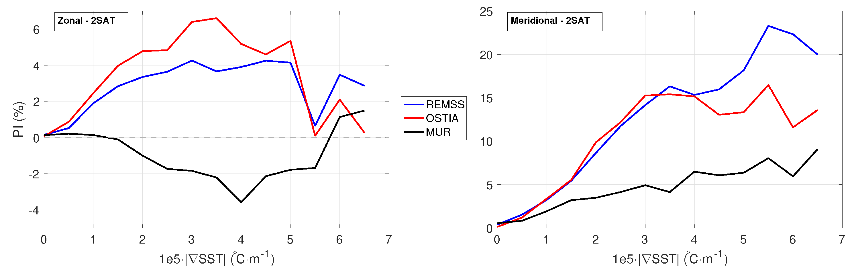
3.1. Reconstruction Based on REMSS Data

In a good agreement with RS18, the OPC computed using the REMSS data exhibit a PI exceeding 20% (up to 24% locally), with better performances for the meridional component of the motion and in the equatorial band. The results indicate that our method is more efficient when applied to low-quality altimetry products, as for the 2SAT case (see also Pascual et al. 2006 [37]). However, still in agreement with RS18, Figure 1 shows that even the 4SAT geostrophic currents do benefit from the optimal combination with SST. Indeed, local maximum improvements range from ≃10% at mid-latitudes to ≃20% in the equatorial band for both the zonal and the meridional currents. Therefore, combining the altimeter-derived currents with SST data is advantageous for both altimetry products based on information from two altimeters (like in the early altimetry era) and more recent versions combining observations from several altimeters. The number of available altimeters can indeed vary from two to four (sometimes five) in the 1993 to 2016 period [36].

On average, the PI of the zonal OPC is lower than in the meridional case. This is easily explained considering the north–south orientation of the nadir-looking altimeter ground tracks, allowing to derive more accurate zonal surface currents via the geostrophic approximation (see, e.g., [16]). However, as previously emphasized by RS18, the optimal reconstruction of zonal ocean currents exhibits poor performance in high latitudes, as indicated by negative PIs that can reach −10%.

3.2. Reconstruction Based on OSTIA Data

Here we present the OPC derivation based on the use of OSTIA SST. The results are given in Figure 2.

The overall performances of the OSTIA OPC are consistent with the reconstructions obtained with the REMSS SST, as shown in Section 3.1. The regional variability of the PI is analogous, indicating that the optimal reconstruction brings larger benefits for the 2SAT case, particularly for the meridional component of the currents and in the equatorial band. However, the OSTIA SST data are smoothed to fulfill operational requirements in numerical weather prediction (https://data.noaa.gov/dataset/dataset/global-sst-sea-ice-analysis-l4-ostia-uk-met-office-global-0-05-daily-2013-present1). According to Equation (2), one may expect average reduced performances than in the REMSS case, mostly due to the smoothing of the spatial SST gradients. Studying the PI as a function of the local $|\nabla \mathrm{SST}|$ (Figure 4) partially confirms this expectation. When the local |∇SST| becomes larger (≃5 to 7$\times {10}^{-5}$${}^{\circ }$C·m${}^{-1}$), the meridional PI of the 2SAT OPC based on OSTIA SST barely exceeds 15% while, for the REMSS 2SAT case, this value can reach 23%.

When considering the zonal component, however, the averaged OPC improvements exceed 6% for the OSTIA case, compared to 4% found with the REMSS SST. An explanation for this behavior will be provided in Section 4.

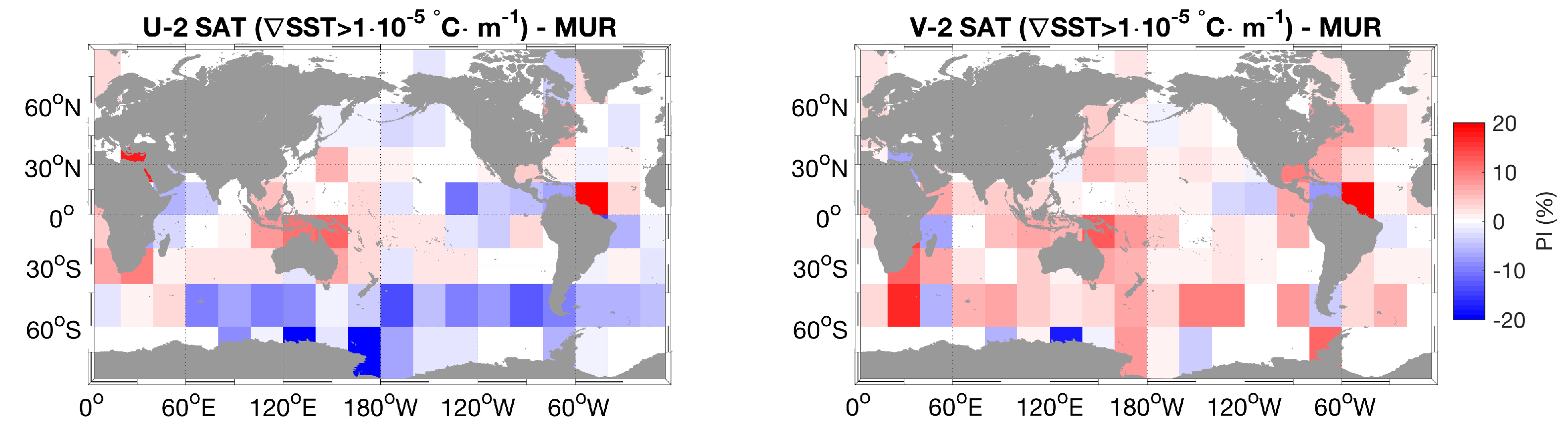
3.3. Reconstruction Based on MUR Data

The OPC derived from the MUR SST are here presented for the 2SAT case. The 4SAT OPC, except for the averaged lower improvements, exhibit similar regional variability and dependence on the local SST spatial gradient magnitude (|∇SST|). The results of 4SAT OPC are provided as Supplementary Materials (Figures S3 and S4).

The MUR OPC showed reduced performances than in the REMSS and OSTIA cases. This is evident from Figure 3 and Figure 4. The zonal degradation area found at high latitudes is even more evident than in the REMSS-based optimal reconstruction. The zonal OPC are degraded compared to the Altimeter currents below 45${}^{\circ }$S as well as in the equatorial Pacific and Indian Oceans. On a global average, the zonal OPC degradation is also confirmed by a negative PI, whose minimum value can go down to ≃−4%, as shown by Figure 4.

The regional and global averaged meridional PIs are lower compared to the OPC computed with the REMSS and OSTIA SSTs. Indeed, the maximum averaged meridional PI barely reaches 9%. This is verified in regions where the local |∇SST| is larger than $\simeq 6.5\times {10}^{-5}$${}^{\circ }$C· m${}^{-1}$ (Figure 4). However, there are regions of the ocean where the local PI can reach 10% to 20% for both components of the motion. This is found in the retroflection area of the Agulhas Current, the North Brazilian current and off Eastern Australia.

4. Discussion and Conclusions

The optimal combination of altimeter-derived currents and SST is a promising technique to improve past and present-day gridded altimetry products. The information contained in high-resolution SST data enables to overcome some of the limitations of the altimeter system for deriving the global ocean circulation. Such limitations are related to the altimeter along-track sampling (with a preferential north–south orientation) and the assumption of geostrophic balance, which fails in low latitudes areas. However, the corrections computed away from the equatorial band by the optimal combination method still lead to mostly geostrophic estimates. As pointed out by RS18, deriving more accurate ageostrophic motions would require the knowledge of the high-resolution source and sink term of the SST dynamical evolution equation, here approximated as a large scale SST temporal derivative. The optimal combination was tested with three global L4 SST datasets: the REMSS, OSTIA and MUR SSTs. These datasets led to different performances in deriving the global ocean OPC. The regional variability of the optimal reconstruction has been described in Section 3, while the global percentage of improvement is here discussed as a function of the local |∇SST| for the 2SAT OPC (Figure 4). The 4SAT case is analogous and is provided as Supplementary Materials (Figure S4).

On average, the PI depends on the magnitude of the local spatial SST gradient. For the meridional PI, all the reconstructions indicate a fairly linear increase up to |∇SST|≃ 4$\times {10}^{-5}$${}^{\circ }$C· m${}^{-1}$. For even larger SST gradients the PI can further increase, as for the REMSS and MUR cases or stabilize as for the OSTIA OPC.

For the zonal case, we get similar behavior in terms of the PI linearity, except a decreasing tendency in areas of highest SST gradients. Interestingly, we notice the enhanced performances of the OSTIA OPC in the 0.2 to 4$\times {10}^{-5}$${}^{\circ }$C· m${}^{-1}$$|\nabla$SST| range, mostly due to improved local performances in the Southern Ocean (Figure 2). In the end, the MUR SST OPC constitute an exception, indicating averaged negative PI for the 2 to 5.6 $\times {10}^{-5}$${}^{\circ }$C· m${}^{-1}$$|\nabla$SST| range. This additional analysis, mostly driven by the knowledge of Equations (2) and (3) indicates how the optimal reconstruction method strongly depends on the local SST gradients. Indeed, in areas of low |∇SST| we can get little to zero improvements. Under these conditions, the optimal reconstruction method cannot correct the background surface currents, as no information related to the upper ocean circulation is available in the spatial patterns of the L4 SST field.

The anomalous behavior of the MUR SST was unexpected. Indeed, the very high nominal resolution of this product should in principle allow a more accurate description of the surface dynamical processes as also emphasized by [44,48] and references therein. In order to further investigate this point, we performed a spectral analysis of the three SST datasets used in our study (Figure 5). Although a thorough quality assessment of the different SST products is out the scope of our paper, this analysis provides a possible explanation for the anomalous behavior of the MUR OPC.

The mean spatial spectral content of the REMSS, OSTIA and MUR SST was analyzed in a test case during wintertime, focusing on scales up to 10 km. This was carried out computing the Power Spectral Density (PSD) via wavenumber spectral analysis in a land-free area of the North Atlantic, on January 1st 2016. Such spatial-temporal selection is due to the results of [49] indicating that, during winter, the submesoscale turbulence is more efficient than in summer. Hence, the expression of the smaller scale structures in SST should be favored under the chosen conditions. The spectral analyses are performed in two distinct boxes of the North Atlantic, both extending longitudinally from 60${}^{\circ }$W to 30${}^{\circ }$W: a first box with latitudinal extent from 30${}^{\circ }$N to 36${}^{\circ }$N and a second from 36${}^{\circ }$N to 40${}^{\circ }$N (the boxes separation is identified by the white line in Figure 5c). In both boxes, the baroclinic Rossby radius of deformation is around 30 km [50]. Investigating scales up to 10 km also enables to capture submesoscale features in the area, whenever they are present.

In the southern box (30${}^{\circ }$N to 36${}^{\circ }$N, see also Figure 5e), the spectra of the REMSS, OSTIA and MUR SST are initially superimposed and so they evolve until scales of ≃200 km. Afterward, the OSTIA spectrum begins to separate, indicating a decreased amount of spatial variance at finer scales, eventually flattening around 50 km. On the other hand, the REMSS and MUR SST exhibit lager PSD than the OSTIA SST, with a dominance of MUR until scales of 15 km, where REMSS is instead quite flat. If we consider the different nature of the three SST datasets described in Section 2, this is the expected spectral behavior of the input SSTs for our application.

If the same spectral analysis is performed in the Northern box (Figure 5c,d), i.e., where the MUR SST looks smoother, the spectral properties of the MUR and REMSS SST are inverted. Indeed, the REMSS spectrum is characterized by larger PSDs at scales lower than 100 km. Therefore, the REMSS SSTs are associated with the finer effective spatial resolution in the Northern Area (36${}^{\circ }$N to 40${}^{\circ }$N). This result is indicating that the global scale OPC based on MUR data can be negatively affected by unequal effective SST resolutions in different areas of the ocean. Visual inspection of the MUR SST fields evidenced that this non uniformity can happen throughout the year in different areas of the ocean. This spectral inconsistency can have drawbacks on the computation of the SST spatio-temporal gradients, in which non physical dynamical structures can be recognized. An example is provided in Figure 6, showing $|\nabla$SST| maps on three different dates in the Gulf Stream, Kuroshio Current and Agulhas Current areas.

On the other hand, the REMSS and OSTIA SSTs did not evidence non-homogeneities in the effective resolution of the L4 fields, being coherent with the example provided in Figure 5 during the period 2014–2016.

However, selecting areas where the MUR SST are spatially uniform, this problem could be overcome and the fine resolution of the SST field can be fully exploited. In Figure 7, we perform a qualitative comparison between the MUR and REMSS OPC in the Agulhas Current. In the chosen area, the following three conditions are satisfied: (i) the SST spectra are comparable with the condition of Figure 5e (not shown); (ii) according to Figure 1 and Figure 3, both the components of MUR and REMSS OPC are improved based on a three-year statistic; (iii) the trajectory of a drifter in correspondence of a SST gradient was available (see also [33]).

It is evident that the MUR SST describe a finer SST gradient than in the REMSS case. Moreover, the gridded current vectors provided by the MUR OPC exhibit a reduced angle with respect to the drifter trajectory in the north-eastern section of the domain (where the drifter time is closer to the date of the Eulerian fields, 25 March 2015).

Concluding, our study can be summarized by the following main items:

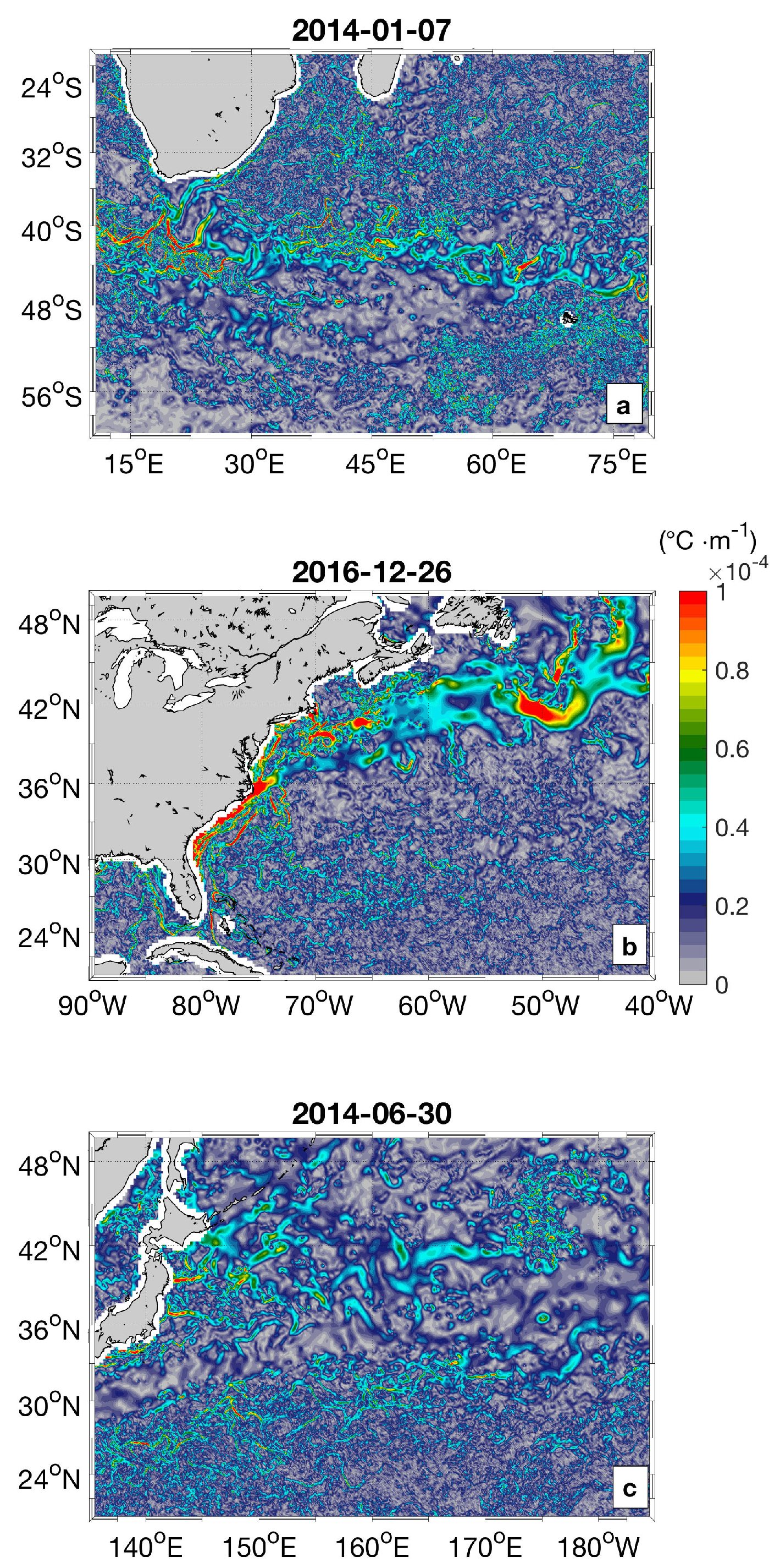
• The derivation of the sea surface currents from space can benefit from the synergy between optimally interpolated space-based Earth observations from multiple platforms, today available at an operational level and with nominal daily and global coverage. Based on recent works [33,47] we attempted to optimize the surface currents retrieval by combining the altimeter-derived geostrophic currents with satellite SST from Infrared (IR) and Microwave (MW) sensors. Our study was based on three different L4 SST estimates: a dataset provided by Remote Sensing Systems, fully based on the optimal interpolation of satellite observations (IR and MW), and two additional datasets based on the optimal interpolation of satellite and in-situ data, i.e., the OSTIA and MUR SSTs.
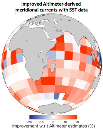
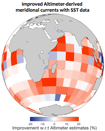
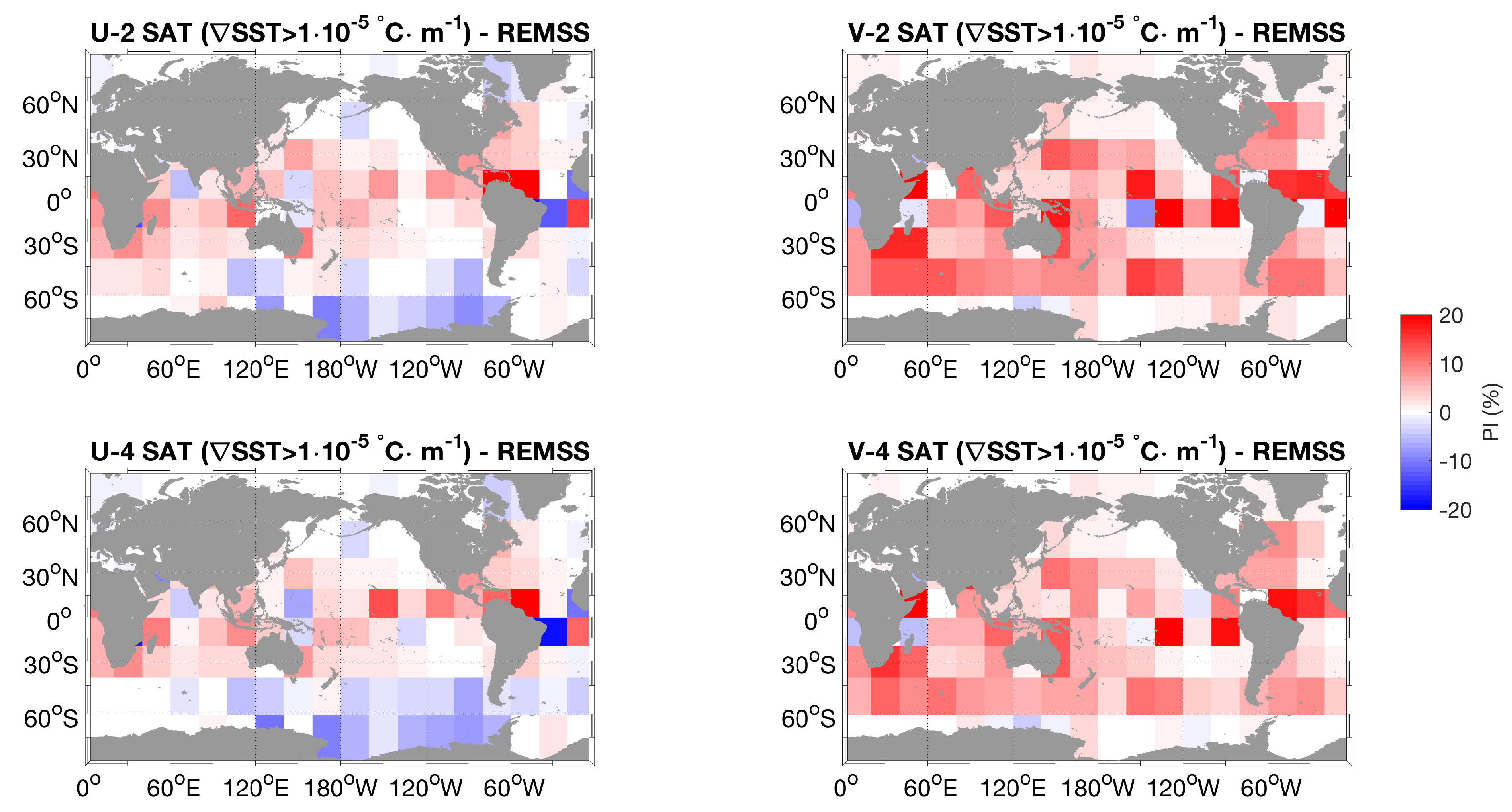
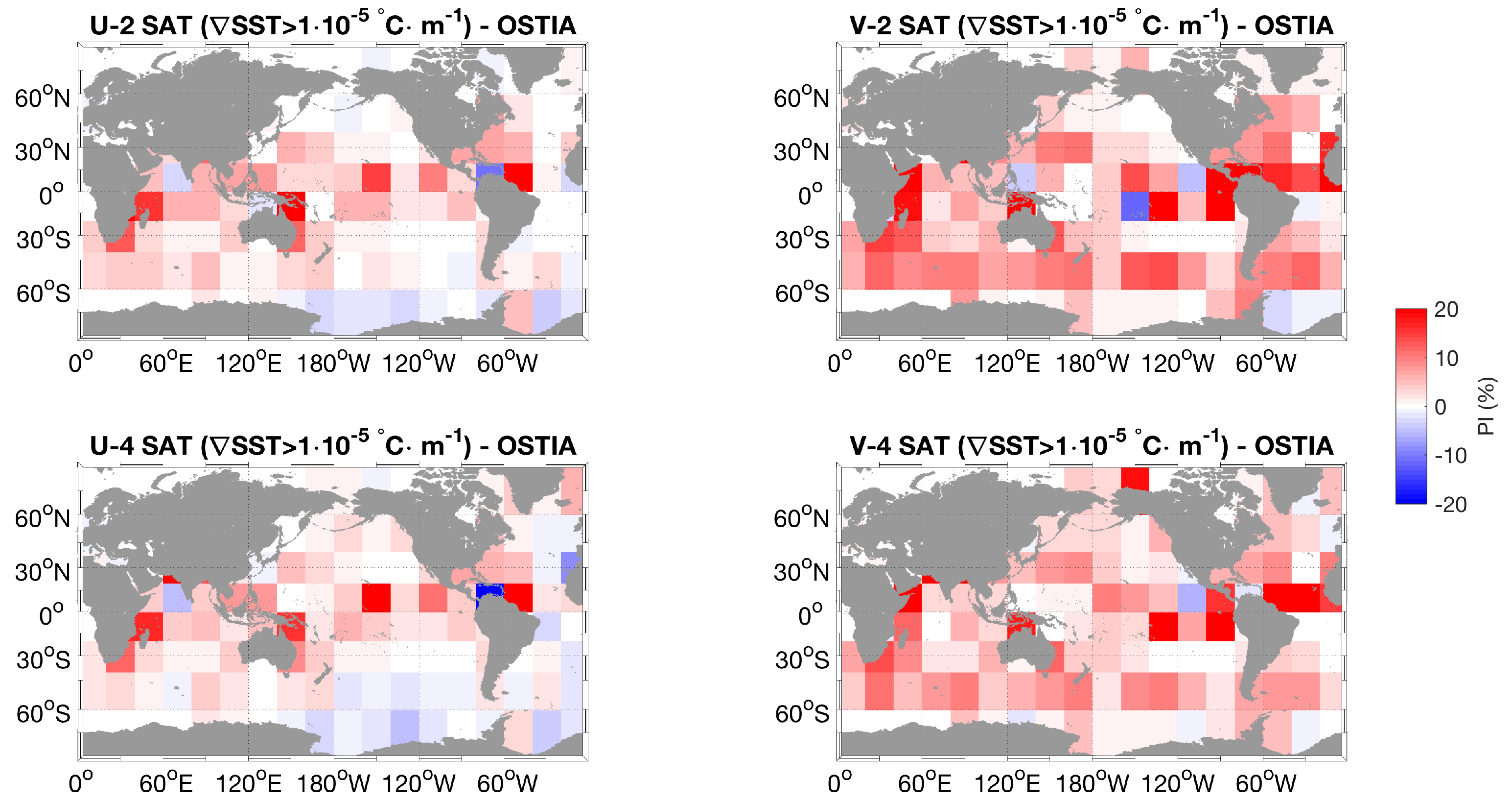
• The REMSS and OSTIA OPC exhibited the best performances, with maximum overall improvements equal to or larger than 15% with respect to the geostrophic estimates (for the meridional flow). This was achieved transferring the high resolution dynamical content of the satellite-derived SST into the coarser resolution geostrophic current estimates [33,34]. However, the OSTIA OPC are characterized by larger improvements than the REMSS OPC in the 0.2 to 4 $\times {10}^{-5}$${}^{\circ }$C· m${}^{-1}$|∇SST| range. This result is due to enhanced performances of the OSTIA OPC in the 45${}^{\circ }$S to 70${}^{\circ }$S latitudinal band. This is illustrated by Figure 1, Figure 2 and Figure 4 and summarized by

  Table 1. REMSS and OSTIA PI in the 45${}^{\circ }$S to 70${}^{\circ }$S latitudinal band. The results are given for the two flow components.

  45${}^{\circ }$S–70${}^{\circ }$S	REMSS	OSTIA
  2SAT - ZONAL PI (%)	−1.35	1.34
  2SAT - MERIDIONAL PI (%)	5.60	6.43
  4SAT - ZONAL PI (%)	−2.48	0.10
  4SAT - MERIDIONAL PI (%)	4.28	4.61

  : the OSTIA OPC partially solve the degradation of the zonal flow in the Southern Ocean, also yielding slightly larger averaged PIs for the meridional flow.
  Most likely, this is due to the larger number of sensors used to build the L4 SSTs as well as the use of in-situ observations in the optimal interpolation procedure. This could optimize the SST estimates at high latitudes, where cloud coverage is often very high and where average intense surface winds degrade the satellite infrared and microwave SST retrievals [51,52]. An additional analysis is provided as Supplementary Materials (Figure S5).
  However, despite the improved performances of the OSTIA OPC compared to the REMSS case, occasional degradations in the polar regions can also occur with the OSTIA SST, as shown in Figure 2. This emphasizes the importance of providing very high quality, high resolution and synoptic SST measurements in those areas, highlighting the strong potential of future ESA satellite missions like the Copernicus Imaging Microwave Radiometer (CIMR) [53] (https://cimr.eu). CIMR will provide global-scale, all-weather, 15 km effective spatial resolution SST observations, also guaranteeing sub-daily coverage at latitudes higher than ±60${}^{\circ }$. All the SST-based applications will benefit from the future CIMR remote sensing capabilities. Applying the RS18 method in high-latitude areas could also benefit from additional oceanic tracers as sea surface salinity. In polar areas, the contribution of salinity in determining the ocean dynamics can be relevant [54].
• The OPC based on the use of MUR very high resolution data, though showing degraded performances at global scale, suggest that fine-scale SST gradients can be retrieved successfully. This is achieved when the MUR SST effective high resolution is homogenous in the study area, mostly indicating a potential for local applications.

Therefore, in order to guarantee an accurate global OPC reconstructions via the method of Piterbarg 2009 and RS18, the L4 SSTs have to contain the signature of fine scale SST gradients and guarantee spatial homogeneity of the optimally interpolated field. In this way, the zonal and meridional SST gradients are not affected by the inhomogeneities like the ones reported in Figure 5 and Figure 6. This work also identifies the RS18 method as a tool for indirect validation of the L4 SST products, allowing to test their dynamical content.

References

1. Hátún, H.; Sandø, A.B.; Drange, H.; Hansen, B.; Valdimarsson, H. Influence of the Atlantic subpolar gyre on the thermohaline circulation. Science 2005, 309, 1841–1844. [Google Scholar] [CrossRef] [PubMed]
2. Bashmachnikov, I.; Neves, F.; Calheiros, T.; Carton, X. Properties and pathways of Mediterranean water eddies in the Atlantic. Prog. Oceanogr. 2015, 137, 149–172. [Google Scholar] [CrossRef]
3. Buongiorno Nardelli, B. Vortex waves and vertical motion in a mesoscale cyclonic eddy. J. Geophys. Res. Ocean. 2013, 118, 5609–5624. [Google Scholar] [CrossRef]
4. Barbosa Aguiar, A.C.; Peliz, Á.; Carton, X. A census of Meddies in a long-term high-resolution simulation. Prog. Oceanogr. 2013, 116, 80–94. [Google Scholar] [CrossRef] [Green Version]
5. Ponte, A.; Klein, P.; Capet, X.; Le Traon, P.; Chapron, B.; Lherminier, P. Diagnosing surface mixed layer dynamics from high-resolution satellite observations: Numerical insights. J. Phys. Oceanogr. 2013, 43, 1345–1355. [Google Scholar] [CrossRef]
6. Frenger, I.; Gruber, N.; Knutti, R.; Munnich, M. Imprint of Southern Ocean eddies on winds, clouds and rainfall. Nat. Geosci. 2013, 6, 608–612. [Google Scholar] [CrossRef]
7. Chenillat, F.; Franks, P.J.; Combes, V. Biogeochemical properties of eddies in the California Current System. Geophys. Res. Lett. 2016, 43, 5812–5820. [Google Scholar] [CrossRef] [Green Version]
8. Siokou-Frangou, I.; Christaki, U.; Mazzocchi, M.G.; Montresor, M.; Ribera d’Alcalá, M.; Vaqué, D.; Zingone, A. Plankton in the open Mediterranean Sea: A review. Biogeosciences 2010, 7, 1543–1586. [Google Scholar] [CrossRef] [Green Version]
9. Olascoaga, M.J.; Beron-Vera, F.J.; Haller, G.; Trinanes, J.; Iskandarani, M.; Coelho, E.; Haus, B.K.; Huntley, H.; Jacobs, G.; Kirwan, A.; et al. Drifter motion in the Gulf of Mexico constrained by altimetric Lagrangian coherent structures. Geophys. Res. Lett. 2013, 40, 6171–6175. [Google Scholar] [CrossRef]
10. Clarke, A.; Li, J. El Nino/La Nina shelf edge flow and Australian western rock lobsters. Geophys. Res. Lett. 2004, 31. [Google Scholar] [CrossRef]
11. Li, J.; Clarke, A.J. Coastline direction, interannual flow, and the strong El Niño currents along Australia’s nearly zonal southern coast. J. Phys. Oceanogr. 2004, 34, 2373–2381. [Google Scholar] [CrossRef]
12. Carlson, D.F.; Clarke, A.J. Seasonal along-isobath geostrophic flows on the west Florida shelf with application to Karenia brevis red tide blooms in Florida’s Big Bend. Cont. Shelf Res. 2009, 29, 445–455. [Google Scholar] [CrossRef]
13. Pisano, A.; De Dominicis, M.; Biamino, W.; Bignami, F.; Gherardi, S.; Colao, F.; Coppini, G.; Marullo, S.; Sprovieri, M.; Trivero, P.; et al. An oceanographic survey for oil spill monitoring and model forecasting validation using remote sensing and in situ data in the Mediterranean Sea. Deep Sea Res. Part II Top. Stud. Oceanogr. 2016, 133, 132–145. [Google Scholar] [CrossRef]
14. Onink, V.; Wichmann, D.; Delandmeter, P.; Van Sebille, E. The role of Ekman currents, geostrophy, and Stokes drift in the accumulation of floating microplastic. J. Geophys. Res. Ocean. 2019, 124, 1474–1490. [Google Scholar] [CrossRef] [Green Version]
15. Cazenave, A.; Palanisamy, H.; Ablain, M. Contemporary sea level changes from satellite altimetry: What have we learned? What are the new challenges? Adv. Space Res. 2018, 62, 1639–1653. [Google Scholar] [CrossRef]
16. Vallis, G.K. Atmospheric and Oceanic Fluid Dynamics; Cambridge University Press: Cambridge, UK, 2006; p. 745. [Google Scholar]
17. Pujol, M.I.; Dibarboure, G.; Le Traon, P.Y.; Klein, P. Using high-resolution altimetry to observe mesoscale signals. J. Atmos. Ocean. Technol. 2012, 29, 1409–1416. [Google Scholar] [CrossRef]
18. Pujol, M.I.; Faugère, Y.; Taburet, G.; Dupuy, S.; Pelloquin, C.; Ablain, M.; Picot, N. DUACS DT2014: The new multi-mission altimeter data set reprocessed over 20 years. Ocean. Sci. 2016, 12, 1067–1090. [Google Scholar] [CrossRef] [Green Version]
19. Ballarotta, M.; Ubelmann, C.; Pujol, M.I.; Taburet, G.; Fournier, F.; Legeais, J.F.; Faugère, Y.; Delepoulle, A.; Chelton, D.; Dibarboure, G.; et al. On the resolutions of ocean altimetry maps. Ocean. Sci. 2019, 15, 1091–1109. [Google Scholar] [CrossRef] [Green Version]
20. Chapron, B.; Collard, F.; Ardhuin, F. Direct measurements of ocean surface velocity from space: Interpretation and validation. J. Geophys. Res. Ocean. 2005, 110. [Google Scholar] [CrossRef]
21. Poulain, P.M. Adriatic Sea surface circulation as derived from drifter data between 1990 and 1999. J. Mar. Syst. 2001, 29, 3–32. [Google Scholar] [CrossRef]
22. Falco, P.; Zambianchi, E. Near-surface structure of the Antarctic Circumpolar Current derived from World Ocean Circulation Experiment drifter data. J. Geophys. Res. Ocean. 2011, 116, C05003. [Google Scholar] [CrossRef] [Green Version]
23. Lumpkin, R.; Özgökmen, T.; Centurioni, L. Advances in the application of surface drifters. Annu. Rev. Mar. Sci. 2017, 9, 59–81. [Google Scholar] [CrossRef] [PubMed] [Green Version]
24. Laurindo, L.C.; Mariano, A.J.; Lumpkin, R. An improved near-surface velocity climatology for the global ocean from drifter observations. Deep Sea Res. Part I Oceanogr. Res. Pap. 2017, 124, 73–92. [Google Scholar] [CrossRef]
25. Capodici, F.; Cosoli, S.; Ciraolo, G.; Nasello, C.; Maltese, A.; Poulain, P.M.; Drago, A.; Azzopardi, J.; Gauci, A. Validation of HF radar sea surface currents in the Malta-Sicily Channel. Remote Sens. Environ. 2019, 225, 65–76. [Google Scholar] [CrossRef]
26. Berta, M.; Griffa, A.; Magaldi, M.G.; Özgökmen, T.M.; Poje, A.C.; Haza, A.C.; Olascoaga, M.J. Improved surface velocity and trajectory estimates in the Gulf of Mexico from blended satellite altimetry and drifter data. J. Atmos. Ocean. Technol. 2015, 32, 1880–1901. [Google Scholar] [CrossRef] [Green Version]
27. Mulet, S.; Etienne, H.; Ballarotta, M.; Faugere, Y.; Rio, M.; Dibarboure, G.; Picot, N. Synergy between surface drifters and altimetry to increase the accuracy of sea level anomaly and geostrophic current maps in the Gulf of Mexico. Adv. Space Res. 2020. [Google Scholar] [CrossRef]
28. Isern-Fontanet, J.; Chapron, B.; Lapeyre, G.; Klein, P. Potential use of microwave sea surface temperatures for the estimation of ocean currents. Geophys. Res. Lett. 2006, 33. [Google Scholar] [CrossRef] [Green Version]
29. González-Haro, C.; Isern-Fontanet, J. Global ocean current reconstruction from altimetric and microwave SST measurements. J. Geophys. Res. Ocean. 2014, 119, 3378–3391. [Google Scholar] [CrossRef]
30. Bowen, M.M.; Emery, W.J.; Wilkin, J.L.; Tildesley, P.C.; Barton, I.J.; Knewtson, R. Extracting multiyear surface currents from sequential thermal imagery using the maximum cross-correlation technique. J. Atmos. Ocean. Technol. 2002, 19, 1665–1676. [Google Scholar] [CrossRef] [Green Version]
31. Qazi, W.A.; Emery, W.J.; Fox-Kemper, B. Computing ocean surface currents over the coastal California current system using 30-min-lag sequential SAR images. IEEE Trans. Geosci. Remote. Sens. 2014, 52, 7559–7580. [Google Scholar] [CrossRef]
32. Warren, M.; Quartly, G.; Shutler, J.; Miller, P.; Yoshikawa, Y. Estimation of ocean surface currents from maximum cross correlation applied to GOCI geostationary satellite remote sensing data over the Tsushima (Korea) Straits. J. Geophys. Res. Ocean. 2016, 121, 6993–7009. [Google Scholar] [CrossRef] [Green Version]
33. Rio, M.H.; Santoleri, R. Improved global surface currents from the merging of altimetry and Sea Surface Temperature data. Remote Sens. Environ. 2018, 216, 770–785. [Google Scholar] [CrossRef]
34. Piterbarg, L.I. A simple method for computing velocities from tracer observations and a model output. Appl. Math. Model. 2009, 33, 3693–3704. [Google Scholar] [CrossRef]
35. Mercatini, A.; Griffa, A.; Piterbarg, L.; Zambianchi, E.; Magaldi, M.G. Estimating surface velocities from satellite data and numerical models: Implementation and testing of a new simple method. Ocean. Model. 2010, 33, 190–203. [Google Scholar] [CrossRef]
36. Taburet, G.; Sanchez-Roman, A.; Ballarotta, M.; Pujol, M.I.; Legeais, J.F.; Fournier, F.; Faugere, Y.; Dibarboure, G. DUACS DT2018: 25 years of reprocessed sea level altimetry products. Ocean Sci. 2019, 15, 1207–1224. [Google Scholar] [CrossRef] [Green Version]
37. Pascual, A.; Faugère, Y.; Larnicol, G.; Le Traon, P.Y. Improved description of the ocean mesoscale variability by combining four satellite altimeters. Geophys. Res. Lett. 2006, 33. [Google Scholar] [CrossRef] [Green Version]
38. Gentemann, C.L.; Donlon, C.J.; Stuart-Menteth, A.; Wentz, F.J. Diurnal signals in satellite sea surface temperature measurements. Geophys. Res. Lett. 2003, 30. [Google Scholar] [CrossRef] [Green Version]
39. Martin, M.; Dash, P.; Ignatov, A.; Banzon, V.; Beggs, H.; Brasnett, B.; Cayula, J.F.; Cummings, J.; Donlon, C.; Gentemann, C.; et al. Group for High Resolution Sea Surface temperature (GHRSST) analysis fields inter-comparisons. Part 1: A GHRSST multi-product ensemble (GMPE). Deep Sea Res. Part II Top. Stud. Oceanogr. 2012, 77, 21–30. [Google Scholar] [CrossRef]
40. Gentemann, C.L.; Meissner, T.; Wentz, F.J. Accuracy of satellite sea surface temperatures at 7 and 11 GHz. IEEE Trans. Geosci. Remote. Sens. 2009, 48, 1009–1018. [Google Scholar] [CrossRef]
41. Donlon, C.J.; Martin, M.; Stark, J.; Roberts-Jones, J.; Fiedler, E.; Wimmer, W. The operational sea surface temperature and sea ice analysis (OSTIA) system. Remote Sens. Environ. 2012, 116, 140–158. [Google Scholar] [CrossRef]
42. Good, S.; Fiedler, E.; Mao, C.; Martin, M.J.; Maycock, A.; Reid, R.; Roberts-Jones, J.; Searle, T.; Waters, J.; While, J.; et al. The Current Configuration of the OSTIA System for Operational Production of Foundation Sea Surface Temperature and Ice Concentration Analyses. Remote. Sens. 2020, 12, 720. [Google Scholar] [CrossRef] [Green Version]
43. Martin, M.; Hines, A.; Bell, M. Data assimilation in the FOAM operational short-range ocean forecasting system: A description of the scheme and its impact. Q. J. R. Meteorol. Soc. 2007, 133, 981–995. [Google Scholar] [CrossRef]
44. Chin, T.M.; Vazquez-Cuervo, J.; Armstrong, E.M. A multi-scale high-resolution analysis of global sea surface temperature. Remote. Sens. Environ. 2017, 200, 154–169. [Google Scholar] [CrossRef]
45. Lumpkin, R.; Grodsky, S.A.; Centurioni, L.; Rio, M.H.; Carton, J.A.; Lee, D. Removing spurious low-frequency variability in drifter velocities. J. Atmos. Ocean. Technol. 2013, 30, 353–360. [Google Scholar] [CrossRef]
46. Rio, M.H.; Santoleri, R.; Bourdalle-Badie, R.; Griffa, A.; Piterbarg, L.; Taburet, G. Improving the Altimeter-Derived Surface Currents Using High-Resolution Sea Surface Temperature Data: A Feasability Study Based on Model Outputs. J. Atmos. Ocean. Technol. 2016, 33, 2769–2784. [Google Scholar] [CrossRef]
47. Ciani, D.; Rio, M.H.; Menna, M.; Santoleri, R. A Synergetic Approach for the Space-Based Sea Surface Currents Retrieval in the Mediterranean Sea. Remote. Sens. 2019, 11, 1285. [Google Scholar] [CrossRef] [Green Version]
48. Vazquez-Cuervo, J.; Gomez-Valdes, J.; Bouali, M.; Miranda, L.E.; Van der Stocken, T.; Tang, W.; Gentemann, C. Using saildrones to validate satellite-derived sea surface salinity and sea surface temperature along the California/Baja Coast. Remote. Sens. 2019, 11, 1964. [Google Scholar] [CrossRef] [Green Version]
49. Callies, J.; Ferrari, R.; Klymak, J.M.; Gula, J. Seasonality in submesoscale turbulence. Nat. Commun. 2015, 6, 6862. [Google Scholar] [CrossRef] [Green Version]
50. Chelton, D.; De Szoeke, R.; Schlax, M.; El Naggar, K.; Siwertz, N. Geographical Variability of the First Baroclinic Rossby Radius of Deformation. J. Phys. Oceanogr. 1998, 28, 433–459. [Google Scholar] [CrossRef]
51. González-Haro, C.; Autret, A.P. Quantifying Tidal Fluctuations in Remote Sensing Infrared SST Observations. Remote. Sens. 2019, 11, 2313. [Google Scholar] [CrossRef] [Green Version]
52. Wentz, F.; Meissner, T.; Gentemann, C.; Hilburn, K.; Scott, J. Remote Sensing Systems GCOM-W1 AMSR2 Daily Data, Environmental Suite on 0.25 Degrees Grid, 2014, Version V.8. Available online: www.remss.com/missions/amsr (accessed on 1 February 2020).
53. Donlon, C.J. Copernicus Imaging Microwave Radiometer (CIMR) Mission Requirements Document; Version 3.0; European Space Agency: Noordwijk, The Netherlands, 2019. [Google Scholar]
54. Roquet, F.; Madec, G.; Brodeau, L.; Nycander, J. Defining a simplified yet realistic equation of state for seawater. J. Phys. Ocean. 2015, 45, 2564–2579. [Google Scholar] [CrossRef] [Green Version]
Figure 1. Percentage of Improvement (PI) (binned in 20 × 20 boxes) of the optimal current (OPC) with respect to the geostrophic estimates (over 2014–2016). Top row: OPC based on the DUACS “2SAT” currents. Bottom row: Optimal currents based on the Data Unification and Altimeter Combination System (DUACS) “4SAT” currents. The input Sea Surface Temperature (SST) is provided by Remote Sensing Systems (REMSS). U and V stand for zonal and meridional currents, respectively.
Remotesensing 12 01601 g001
Figure 2. Same as Figure 1. The input SST is Operational Sea Surface Temperature and Sea Ice Analysis (OSTIA).
Remotesensing 12 01601 g002
Figure 3. Same as Figure 1. The input SST is Multiscale Ultra-high Resolution (MUR).
Remotesensing 12 01601 g003
Figure 4. PI as a function of the local |∇SST| for the zonal and meridional OPC. Red: OPC with REMSS SST; Blue: OPC with OSTIA SST; Black: OPC with MUR SST.
Remotesensing 12 01601 g004
Figure 5. Left: (a) OSTIA, (b) REMSS and (c) MUR SST, 1 January 2016, North Atlantic. Right: Corresponding mean zonal spatial spectra. (d) Northern box (36 N to 40 N), (e) Southern box (30 N to 36 N) (the x axis is also expressed in km). The white line is referenced in Section 4.
Remotesensing 12 01601 g005
Figure 6. (a) | SST| in the Agulhas Current area; (b) same, in the Gulf Stream area; (c) same, in the Kuroshio Current area. The images correspond to the |∇SST| based on MUR SST on three different dates indicated in the panels.
Remotesensing 12 01601 g006
Figure 7. Optimal current vectors (black arrows) based on the REMSS and MUR SST reconstruction. The SST field is given in colors. The trajectory of a drifter is given in white. The magenta and black dots respectively stand for the buoy position from 25 March 2015 (00 UTC) to 26 March 2015 (00 UTC). The gridded fields represent 25 March 2015.
Remotesensing 12 01601 g007