Article

A Cloud-Based Evaluation of the National Land Cover Database to Support New Mexico’s Food–Energy–Water Systems

1
Water Science and Management Program, New Mexico State University, Las Cruces, NM 88003, USA
2
New Mexico Water Resources Research Institute, New Mexico State University, Las Cruces, NM 88003, USA
3
Department of Animal and Range Sciences, New Mexico State University, Las Cruces, NM 88003, USA
4
National Forest Monitoring Team, the Food and Agriculture Organization of the United Nations, 00153 Rome, Italy
5
Department of Fish, Wildlife and Conservation Ecology, New Mexico State University, Las Cruces, NM 88003, USA
*
Author to whom correspondence should be addressed.
Remote Sens. 2020, 12(11), 1830; https://doi.org/10.3390/rs12111830
Submission received: 29 March 2020 / Revised: 25 May 2020 / Accepted: 2 June 2020 / Published: 5 June 2020

Abstract

:
Accurate estimation of land use/land cover (LULC) areas is critical, especially over the semi-arid environments of the southwestern United States where water shortage and loss of rangelands and croplands are affecting the food production systems. This study was conducted within the context of providing an improved understanding of New Mexico’s (NM’s) Food–Energy–Water Systems (FEWS) at the county level. The main goal of this analysis was to evaluate the most important LULC classes for NM’s FEWS by implementing standardized protocols of accuracy assessment and providing bias-corrected area estimates of these classes. The LULC data used in the study was based on National Land Cover Database (NLCD) legacy maps of 1992, 2001, 2006, 2011, and 2016. The analysis was conducted using the cloud-based geospatial processing and modeling tools available from System for Earth Observation Data Access, Processing, and Analysis for Land Monitoring (SEPAL) of the Food and Agricultural Organization. Accuracy assessment, uncertainty analysis, and bias-adjusted area estimates were evaluated by collecting a total of 11,428 reference samples using the Open Foris Collect Earth tool that provided access to high spatial and temporal resolution images available in Google Earth. The reference samples were allocated using a stratified random sampling approach. The results showed an overall accuracy that ranged from 71%–100% in all six study counties. The user’s and producer’s accuracy of most LULC classes were about or above 80%. The obtained bias-adjusted area estimates were higher than those based on pixel counting. The bias-adjusted area estimates simultaneously showed decreasing and increasing trends in grassland and shrubland, respectively in four counties that include Curry, Roosevelt, Lea, and Eddy during the 1992–2016 period. Doña Ana county experienced increasing and decreasing trends in grassland and shrubland areas, respectively. San Juan county experienced decreasing trends in both grassland and shrubland areas. Cultivated cropland areas showed decreasing trends in three counties in southeast NM that rely on groundwater resources including Curry, Roosevelt, and Lea. Similarly, cultivated cropland areas showed increasing trends in the other three counties that rely on surface water or conjunctive use of surface and groundwater resources including San Juan, Doña Ana, and Eddy. The use of SEPAL allowed for efficient assessment and production of more accurate bias-adjusted area estimates compared to using pixel counting. Providing such information can help in understanding the behavior of NM’s food production systems including rangelands and croplands, better monitoring and characterizing NM’s FEWS, and evaluating their behavior under changing environmental and climatic conditions. More effort is needed to evaluate the ability of the NLCD data and other similar products to provide more accurate LULC area estimates at local scales.

Graphical Abstract

1. Introduction

Natural ecosystems have pivotal roles in providing water, energy, land, and food for humans’ societal and economic development [1,2]. In other words, as complex systems, these natural ecosystems are the epicenter of the Food, Energy, and Water systems (FEWS). Anthropogenic activities including urbanization, industrial development, agriculture modernization, international and regional trade, however, can modify natural ecosystems and impact the sustainability of FEW resources [3,4,5,6]. A recent special report by the Intergovernmental Panel on Climate Change (IPCC) on climate change and land indicated that humans modify more than 70% of the ice-free land surface [7]. In this regard, land use activities, including those for food production, which use ¼ to ⅓ of global land’s potential primary production and the shifts in land management, constitute the main factors that change and transform significant proportions of the Earth’s environment and also directly contribute to climate change [1,7]. Most of the natural ecosystems (i.e., forests, grasslands, and wetlands) conversions were associated with shifts to agriculture and driven by the increase in human population and per capital consumption of resources over the last three centuries [8,9,10]. In the contiguous United States (US), about 28% out of the 3.1 million square miles of land have been profoundly changed over time for croplands and pasture (22%) and settlement (6%) as indicated by in the US’s Fourth National Climate Assessment (NCA4) [1]. Understanding the role of these natural ecosystems spatially and temporally is important to assess their ability to continue providing sustainable services to humans’ wellbeing and the environment [2]. Therefore, their robust mapping, assessment, and development of spatially descriptive information for monitoring and policy implementation purposes are critical [10].
The currently available satellite data archives and advanced computational algorithms have enabled efficient land use/land cover (LULC) mapping and monitoring at regional, continental, and global scales. Moreover, the classification of land surface features based on satellite data into LULC thematic maps has provided an improved understanding of the complex relationships between human and biophysical systems, enhanced the ability to provide reasonable predictions of future conditions, and allowed the development of mitigation and adaptation plans and practices [11,12,13]. Such information is critically needed, especially over regions that are heavily dependent on natural cover resources for food production while also facing naturally and anthropogenically caused changes, such as New Mexico (NM). The recent US NCA4 report and the World Resources Institute’s water stress index suggested that the NM state is currently under, and will most likely continue facing, extreme water stress, drought, heat waves, and wildfires conditions that can affect rangelands, cropland, and livestock production that can appear at local scales [14,15].
According to [16], more than 90% of NM’s land is considered as rangeland used mainly for livestock grazing. Arid rangelands including grassland ecosystems in the southwest US, particularly NM, have been degraded and encroached by woody shrubs, consequently leading to a decline in grazing capacity, water availability, and species diversity [17,18,19,20]. Thus, NM’s rangelands ecosystems significantly contribute to the state’s food production systems, as represented mainly by the livestock industry, and are socioeconomically important to New Mexican’s livelihood, cultural values, and generally to the state’s economy. These natural ecosystems are one of the main constituents of strongly interconnected FEWS in the state. The resiliency of NM’s FEWS is challenged when these natural systems are affected by increased socioeconomic demands due to population growth and persistent drought events [21].
Generally, Nexus of FEWS focuses on understanding the relationships between food, energy, and water (FEW) resources with respect to their interconnected utilization, production, and security. It should be noted that the objective of this analysis was not to present an implementation of a FEW Nexus approach. Rather, it was more focused to generate LULC change analysis to support and advance the understanding of these inherent interconnected relationships, qualitatively and quantitatively. More details about the application of the FEW Nexus approach relevant to New Mexico can be found in [18,20,21,22,23]. Changes in LULC classes due to natural and/or anthropogenic processes, such as conversion to croplands, loss of grassland, and woody plant encroachment, can act as drivers of the FEW Nexus behavior, for example, by quantitatively affecting food production, water use, and energy consumption. Thus these changes in turn can introduce significant impacts on FEW Nexus complexity, uncertainty, and synergy [24,25] that need to be evaluated with high level of confidence. Therefore, accuracy assessment of LULC maps can support FEW Nexus studies by providing more effective and efficient evaluation of potential associated changes in FEW Nexus behavior; providing a baseline analysis; and support optimization of FEW resources at multiple spatial scales.
Some previous efforts have been made to account for some of the changes in these ecosystems in the southwest US particularly in the Jornada Experiment Range (JER) [26,27,28,29] and Chihuahua Desert Range (CDR) [27,28,29]. These studies used remote sensing and land survey tools to evaluate vegetation response to changes in hydrological fluxes [29]; detection of vegetation dynamics; and monitoring of long-term vegetation changes [17,26,27]. In one of the studies that was conducted in NM during 1858–1998, ecoregions were evaluated as basic spatial unit [27]. The study by [27] indicated that dominant changes in South Central Semiarid Prairies were from agriculture to grassland and grassland to Agriculture. Moreover, the most common conversion in the Chihuahua Desert ecoregion during 1973–2000 period was from grass/shrubland to mining, developed to agriculture, and agriculture to grass/shrubland [26]. These studies, however, were either ecoregion based or restricted to research area boundaries, which limited our understanding the effects of the LULC changes on FEWS resources at county levels. Thus, consistent datasets and evaluations methods are needed to address such issues.
For a more consistent change evaluation, the remote sensing-based thematic mapping products of the US—the National Land Cover Database (NLCD), can provide spatially explicit and reliable information about LULC change over a period of time. The NLCD datasets, that were used in this analysis, are further expected to be available to continue providing either the same or enhanced products in the future at the national scale [30]. Existing land cover maps have some degree of uncertainty and inconsistency in their classification as indicated in their reported user’s, producer’s, and overall accuracies due to various sources of errors [31]. These accuracies are typically reported at the national scale. Absence of accuracy reports and robust approach for accuracy and area estimation at the county scales is the main roadblock to tap the advantage of these datasets. Therefore, the NLCD maps need to be assessed for their accuracy at local scales to support related land management decisions using appropriate sampling and assessment methods. Based on such assessment, the NLCD maps can then be effectively utilized to provide relevant information needed (e.g., area estimates of LULC changes) to monitor FEWS in semi-arid regions such as New Mexico.
Generally, the NLCD is a product provided by the Multi-Resolution Land Characteristics (MRLC) Consortium—a group of US federal agencies. So far, the released legacy NLCD products included land use and land cover change, land cover thematic maps, impervious surface and tree canopy for 1992, 2001, 2006, 2011, and 2016. A new generation of NLCD product was recently released with relatively higher temporal resolution (at two- to three-year intervals) that cover the period between 2001 and 2016 [30]. Different classification methods have been utilized to develop these products with variable levels of accuracy. For example, combined procedures of unsupervised classification, interpretation, labeling and confusion reduction by the construction of logical or threshold models were used to develop NLCD 1992 [32]. A decision and regression tree classification algorithm was used to develop NLCD 2001 based on satellite images and ancillary layers [33]. The NLCD 2001 was the first product to include percent of tree canopy and impervious areas. The NLCD of 2006 which included a land cover product and change between 2001 and 2006 was developed based on a Multi-Index Integrated Change Analysis (MIICA) and it was the first in its kind to provide a wall-to-wall cover change database for the conterminous US [34]. For the NLCD 2011, Comprehensive Change Detection Method (CCDM) was used to provide products of land cover, impervious areas, and change for three time periods that included 2001, 2006, and 2011 [35,36]. Decision tree classification, hierarchical theme post classification, and biophysical parameters modeling were used to develop the NLCD of 2016 [30].
The accuracy assessment reports of the NLCD thematic maps emphasized the need for, and provided, documentation of products’ quality and reliability at the national, zonal, and regional levels [30,33,37,38,39]. Briefly, NLCD thematic maps exhibited overall accuracy (OA) of 40%–70% (Anderson Level II) in eastern and western US [37,38], 70%–70.5% [40], 78% (Anderson Level II) [34], 88% [39], and 71%–97% [30] in year 1992, 2001, 2006, 2011, and 2016, respectively. The NLCD maps of 2001 and 2006 that were released in 2014 exhibited better OA of 89% compared with earlier releases [39]. These OA values showed consistent improvement over the years indicating the advancements made in terms of efficient image processing algorithms to produce improved LULC mapping, classification, and change detection. However, the provided reports of accuracy assessment lacked information about area estimates, the corresponding uncertainties, and the OA at county levels. This lack of information has resulted in a limited use of NLCD maps at these local scales. Consequently, land cover products were not frequently used in monitoring FEWS components related to land cover types (i.e., shrubland, grassland, and cultivated cropland) during production, conservation, utilization, and management decisions at county level. Therefore, a more consistent accuracy assessment of LULC maps is needed to provide information about their uncertainty and area estimates to support county level applications.
To appropriately address these needs, this analysis highlighted the use and capabilities of a recently developed LULC mapping and change analysis platform called the System for Earth Observation Data Access, Processing, and Analysis for Land Monitoring (SEPAL) [41]. The use of the SEPAL platform was driven by the fact that the multitemporal nature of LULC mapping and change detection require using standardized and efficient methods and protocols of data entry, image interpretation, accuracy assessment, and area estimation in order to provide a consistent accuracy assessment [38]. The SEPAL platform, as it was developed by the Food and Agriculture Organization (FAO) of the United Nations, uniquely provides the mean efficient standardized protocols with an enhanced cloud-based geospatial infrastructure that enables quick accessing, querying, and processing of historical remote sensing datasets that are available from multiple sensors. This includes, for example, Landsat and Sentinel-2 as well as Light Detection and Ranging (LiDAR) data. SEPAL integrates Google Earth Engine (GEE) with its cloud-based computations and storage capabilities, open source software—ORFEO Toolbox of the National Center for Space Studies (CNES), Paris, France based on a project initiated in 2006 for remote sensing images processing, R Studio Server, R Shiny Server, SNAP Toolkit, and Open Foris Geospatial Toolkit [42] to provide a toolset dedicated for land monitoring for stratified sampling, response design, and analysis for consistent accuracy assessment and uncertainty analysis [43]. This platform has more than ten application modules from which the Stratified Area Estimator module with its Design and Analysis submodules is implemented on the cloud for sampling and analysis of LULC maps following the guidelines of [44]. SEPAL also has the capability to quickly and easily assess the accuracy and evaluate the uncertainty of readily available thematic maps [43].
The main goal of this analysis was to evaluate the most important LULC classes from the perspective of understanding FEWS by implementing standardized protocols of accuracy assessment and providing bias-corrected area estimates of these classes. The analysis was performed on the NLCD data using the SEPAL tools—a cloud computing platform. The quality of NLCD maps was assessed at the county level to determine the uncertainties of LULC area estimates of the classes that are relatively important to NM’s FEWS management decisions that include shrubland, grassland, and cultivated cropland for the period 1992–2016. The specific objectives were to estimate the user’s, producer’s, and overall accuracies; bias-adjusted area estimates; and provide estimates of confidence intervals as a measure of the related uncertainties over six study counties in New Mexico.

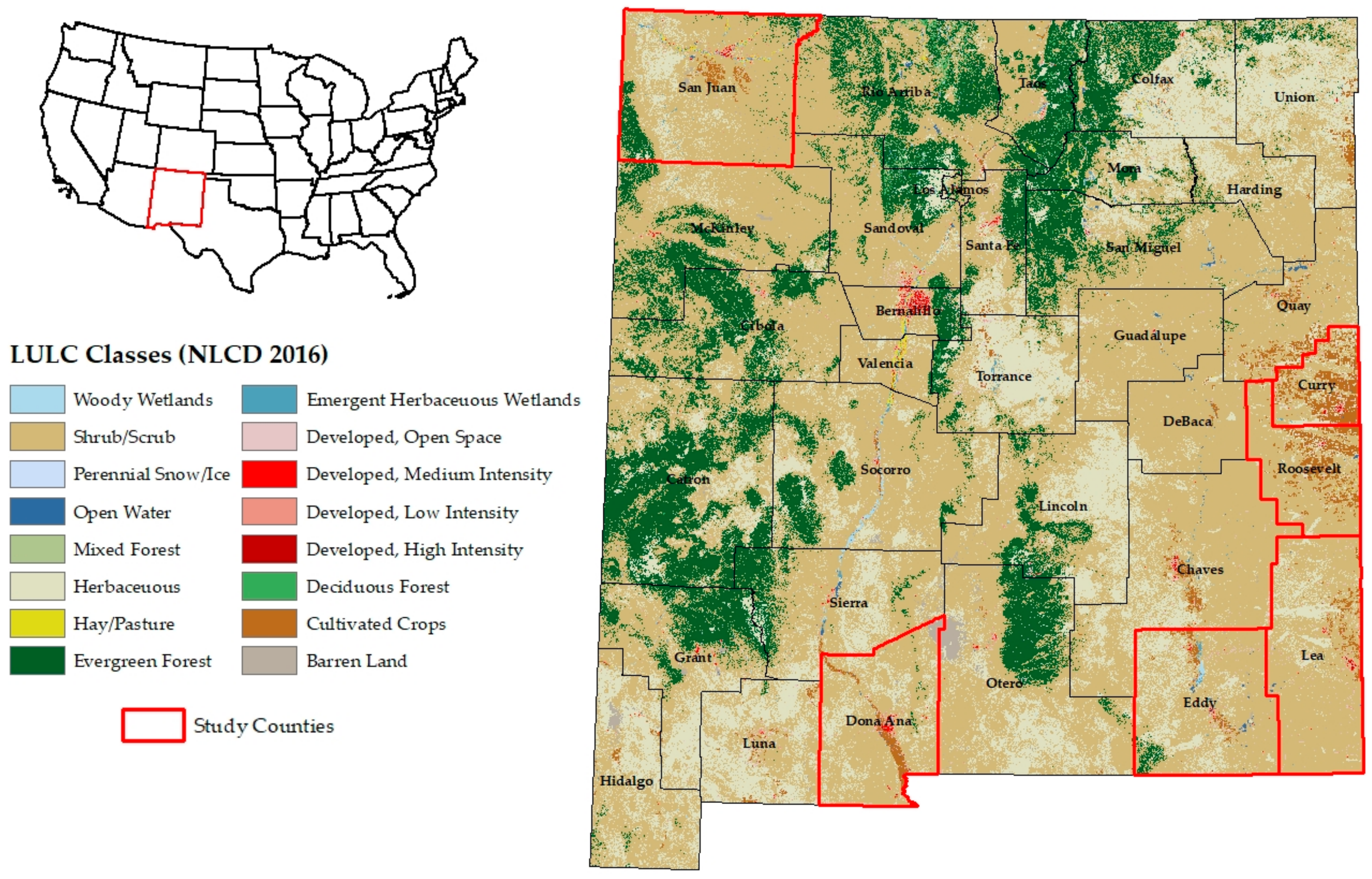
2. Study Area and Data
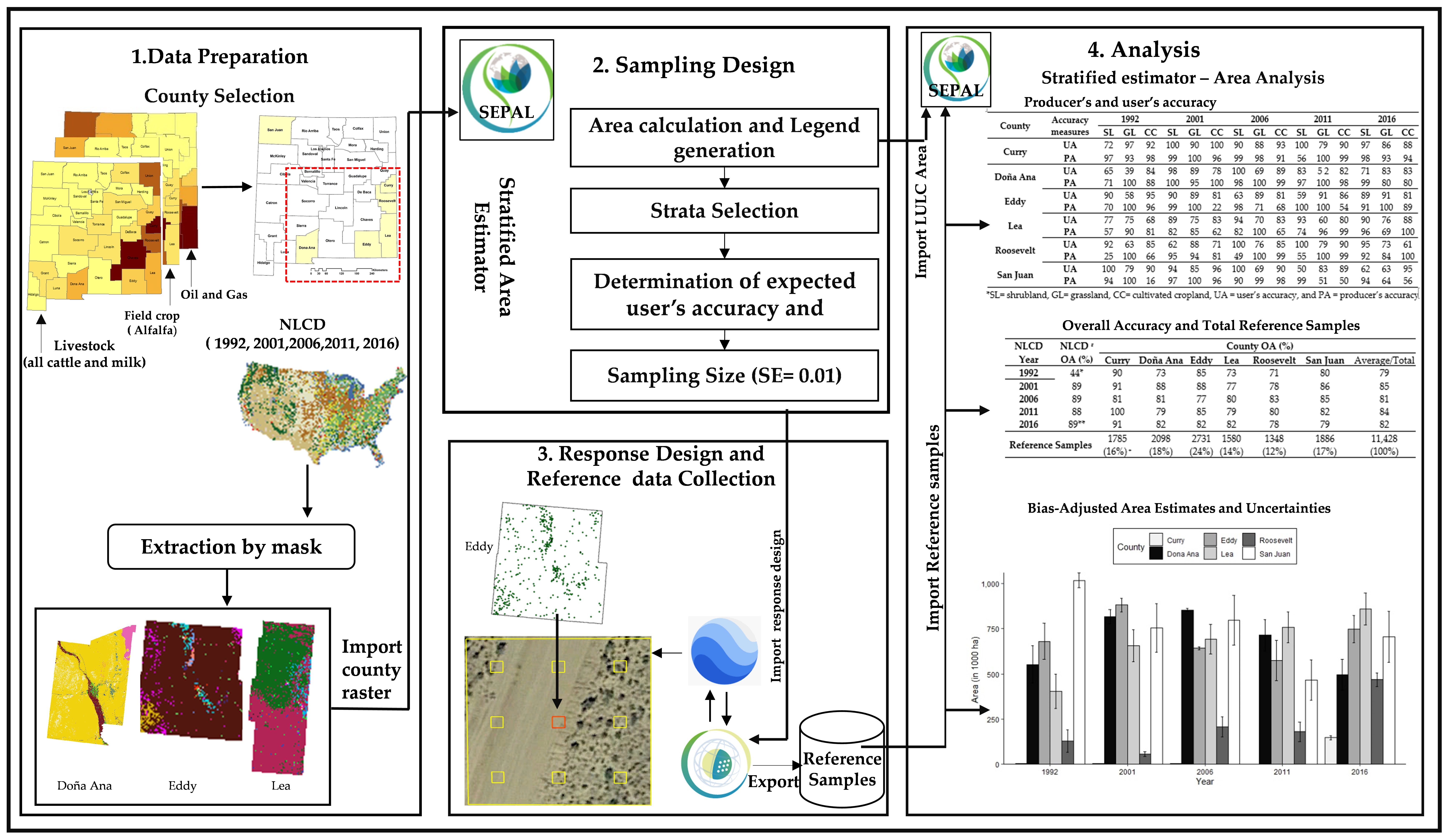
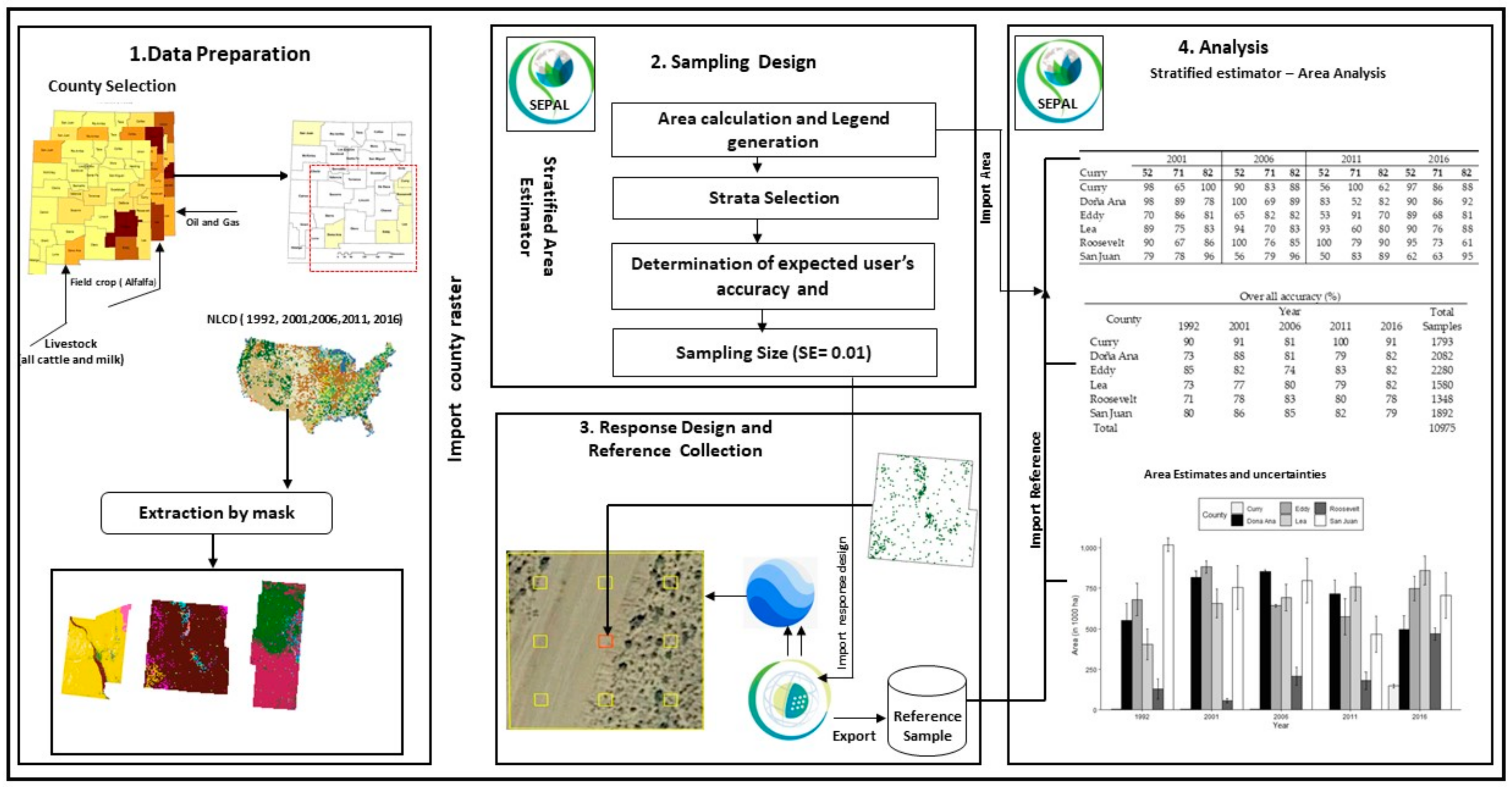
The study area consisted of six counties that were selected mainly based on the dominant availability of food and energy resources in New Mexico. The counties included San Juan (14,344 km2), Curry (3647 km2), Roosevelt (6358 km2), Lea (11,3881 km2), Eddy (10,872 km2), and Doña Ana (9880 km2) (Figure 1). The selected counties cover an area of ~ 20% (56,481 km2) of NM’s total area (314,918 km2). The natural biophysical properties of these counties including ground elevation and vegetation cover vary throughout the study area. The ground elevation varies from 855 m above mean sea level (amsl) in southern NM to 2862 m (amsl) in northcentral NM [45]. The predominant vegetation cover in the study area consists of shortgrass prairie, pinyon juniper woodland, sagebrush grassland, and deserts [25]. NM’s climate is characterized by high and low bi-annual precipitation patterns during summer and winter, respectively, and have recently seen increased temperature trends since 1970s [14,19,20].
Five different datasets have been used. The first dataset is the single-date NLCD thematic maps of 1992, 2011, 2006, 2011, and 2016 that were acquired from MRLC data repository [46]. The second dataset comprised of the ancillary data related to NM’s agriculture and energy production that was used in the selection of the study counties. Agricultural production related to beef cattle, milk, and alfalfa production was obtained from the US Department of Agriculture National Agricultural Statistics Service (USDA–NASS) [47]. Energy production related to crude oil and natural gas production was obtained from the US Energy Information Administration (EIA) and Oil Conservation division (OCD) [48,49]. The third dataset included remote sensing images and their derived indices. This dataset was critical in assessing the NLCD (1992–2016) maps as it allowed the collection of accurate reference data. Medium to very high spatial resolution satellite images including those from Digital Glob (IKONOS and QuickBird), SPOT, Copernicus Sentinel, and Landsat were facilitated from Google Earth (GE), and Bing Maps using Collect Earth (CE) tool, which is one of the Open Foris open source tools [50,51,52]. Aerial photos were also used from the GE archives. Additionally, CE tool also allows to generate and access vegetation indices such as the Normalized Difference Vegetation Index (NDVI), Enhanced Vegetation Index (EVI) and Normalized Difference Water Index (NDWI) from high temporal resolution imagery from Landsat and MODIS archived in GEE. One of the advantages of accessing these datasets from GEE and GE through the CE tool is that some of these data are freely available while the others (especially those with high spatial resolution) require some fees. Thus, the CE tool provides visual accessing and processing of all these datasets without the need to incur any fees or use local resources to store and process the data. it should be noted that due to the limited availability of high to very high spatial resolution data prior to year 2000, relatively lower resolution data (e.g., from Landsat) have been minimally utilized to collect sample and identify LULC classes with additional cautious. It is typical to experience some challenges in identifying surface features using relatively lower spatial resolution data such as those from Landsat. The interpretation and, thus, the classification of any reference samples collected from such datasets (especially over heterogeneous surfaces) can have lower confidence, and eventually affect the accuracy assessment results. The fourth dataset describes NM’s climate, which includes Palmer Drought Severity Index (PDSI), and temperature anomalies for the period 1885–2019 were acquired from West Wide Drought Tracker [53]. Finally, the reference dataset were collected to assess the multitemporal NLCD maps using the CE tool [52]. The CE tool provides a semi-automated labeling and reference data collection technique.

3. Method

The methodology followed in this analysis to assess the accuracy of the LULC maps and provide area estimates and the related uncertainties of the LULC classes consisted of (1) data preprocessing, (2) reference data collection, and (3) assessment and area estimation (Figure 2). The data preprocessing included the extraction of the NLCD maps for the six selected counties and their organization in SEPAL platform. The reference data collection described the sampling technique including the process of stratification, selection of sampling design, sampling unit, and sample size. Finally, an analysis was performed to evaluate the agreement between reference data and map data using a confusion matrix and to estimate LULC areas for the different cover types based on the accuracy results (i.e., with the corresponding confidence interval (CI) as a measure of the uncertainty). The study then further compared the observed trend in LULC with the occurrence of drought events and temperature anomalies to highlight any potential relationships between them.

3.1. Data Preprocessing

The six counties that contributed the most to NM’s agriculture and energy production were listed in Table 1. Based on annual agriculture production for year 2017 [47], food production represented here by the number of all cattle and milk production as well as hay production (i.e., alfalfa and mixture) were considered. Year 2017 data were used to capture counties that maintained reasonable food and energy production following drought and price change [18]. The six counties that contributed the most to beef cattle and milk included Curry, Roosevelt, Lea, Eddy, Doña Ana, and San Juan (Table 1). All selected counties, except San Juan, accounted for ~ 65% of NM’s total milk production. About 30% of NM’s hay production was accounted for by San Juan, Curry, Roosevelt, and Eddy counties. The NM state accounted for 5% and 4% of the US total crude oil and natural gas production, respectively [34]. Eddy, Lea, and San Juan counties accounted for about 98% of NM’s crude oil production. Natural gas was largely produced in San Juan (27%), Eddy (28%), and Lea (23%) [48,49]. Moreover, as these selected counties were leading in livestock and energy production, they also significantly contribute to NM’s economy (Figure 1). Based on this selection, the NLCD maps were then clipped by the county to drive the analysis in SEPAL.

3.2. Reference Data Collection

To perform an effective accuracy assessment and determine uncertainty of area estimates of single-date NLCD thematic maps, high quality reference data was collected using recommended sampling approach [44] which involved the selection of appropriate sampling design, sampling unit, and sample size. In order to collect reference samples (referred to herein also as reference data), stratified random and proportional sampling design was used for which the strata were defined by the LULC classes. The process of stratification ensures a sufficient amount of reference samples even for rare classes or small fraction change classes. Then, the reference samples were randomly distributed in each stratum within the cloud-computing platform (i.e., SEPAL) [44]. The total sample size (n) for each county was calculated following [54] as described in Equation (1).
n = W i   S i 2 S ô 2 + 1 N W i S i 2   w i   S s i S s ô   2
where n = number of reference samples for each county, N is the number of pixels of the NLCD raster subset (i.e., the Spatial unit), S(ô) the standard error of the estimated overall accuracy that the research would like to achieve [44], Wi the mapped proportion area of class i, and Si the standard deviation of the stratum i, Si = U i 1 U i ,where Ui is a conjectured value of user’s accuracy of a land cover class i [44].
The number of reference samples for each LULC class was selected based on area proportions of mapped area and expected (i.e., conjectured) level of accuracy (user’s accuracy) from the perspective of map users and ground-based knowledge. The sampling unit (i.e., spatial size of the reference samples) was chosen by considering the minimum mapping unit (MMU) of the NLCD (0.45 ha) with a 3x3 pixels block in which nine sample squares (5 × 5 m squares) were placed at a distance of 20 m from each other leaving a 15 m margin from the outer edges (Figure 2).
The ratio of squares intersecting with a particular class to total sample squares were used as percent to calculate the proportion of each LULC class. The sample size of each of the six counties was selected based on the proportion of each LULC class determined by majority rule. Finally, the response design was developed in SEPAL [44] using the above mentioned sampling technique to determine the agreement between the map (i.e., NLCD) and the reference data [55]. The reference samples were visually interpreted and labeled using Anderson classification II [56] scheme of NLCD maps. To ensure sufficient number of samples for each LULC class, Deciduous Forest and Evergreen Forest subclasses were aggregated to Forest class. As a result, NLCD map labels were cross walked or translated to label the reference data with dominant LULC class.
The collection of reference data was performed by coupling the CE tool [57], Google Earth images, and GEE platform which provided a long time series of NDVI images as well as the multispectral Landsat images. The use of such robust reference datasets can be very effective for the future assessment applications due to their well-maintained reference sample ID, NLCD code, reference code, and date in the Collect Earth tool.

3.3. Assessment and Area Estimation

The assessment phase included the comparison of map data and reference data for generating the error matrices representing the accuracy measures of each LULC class as well as area estimation and associated uncertainties (i.e. expressed through confidence interval). The error matrix consisted of the map class j (rows) and reference class i (column). The overall accuracy (OA) was calculated using Equation (2) as described in [44] as it explains the proportion of area classified correctly, hence refers to the probability that a randomly selected location on the map data was classified correctly [55]. In other words, Equation (2) is a measure of the agreement between the map data and reference samples. The user’s accuracy (or commission error) of a class refers to proportion of area mapped as class i and labeled as class i in the reference samples (Equation (3)). On the other hand, the producer’s accuracy (or omission error) refers to the proportion of area that is reference class j and class j in the map class (Equation (4)). It is the probability that class j on the ground is mapped as the same class j (Table 2).
O = j = 1 i p j j
U i = P p i i p i .
P p j = p j j p . j
where O is the overall accuracy, pjj the proportional area of LULC class classified as class j and reference class j, Ui the is the user’s accuracy, pii the proportion of area for a land cover classes that has map class i and reference class i, pi the total reference sample allocated in class i, pj the Producer’s accuracy, p.j the total reference sample collected of each class j.
The accuracy measures were used to derive the area and change area estimates by adjusting the map bias. The bias-adjusted area estimates were obtained first by calculating area proportion ( p ^ i j ) using Equation (5).
p ^ i j = W i n i j n i .
where p ^ i j is the estimated area proportion, Wi is the area proportion of map class i (i.e., fraction of map area of class i divided by the total area of all classes in the county), nij is the sample count at cell (i, k) in the error matrix, ni the total sample in map class i.
The output of the matrix from Equation (5) was translated to weighed proportional error matrix (i.e. p ^ i j multiplied by total area of a county). Then, the adjusted area was obtained by adding each columns of the matrix using Equation (6).
p ^ . k = j = 1 q p ^ i k  
where p ^ . k is the sum of estimated area proportions of class k derived from the reference classification and p ^ i k is proportional area derived from reference sample (p.k).
The standard error of the bias-adjusted area estimates was calculated using stratified estimator of proportional area following Equation (7) [44]. Finally, the area estimate of NLCD classes were calculated by multiplying the total map area (A) of a class by the standard error ( p ^ . k ) . The standard error of the estimated class area S ( A ^ k ) was calculated using Equation (8).
S p ^ . k   = i W i 2 n i k n i 1 n i k n i n i 1 = i W i p ^ . i k   p ^ . i k 2 ˙ n i 1 ˙
where nik is the sample count at cell (i,k) in the error matrix.
S ( A ^ k ) = A   *   S ( p ^ . k )
where S ( P ^ k ) is the standard error of proportional area.
The CI value, is a main measure of uncertainty and how well the area was estimated or adjusted. A 95% confidence interval was calculated for the bias corrected area estimates. Moreover, the percentage of CI was calculated by dividing the estimated 95% CI (in ha) by the bias corrected area estimates (AE).

3.4. SEPAL: A Cloud-Based Land Monitoring Platform

In SEPAL [41], the Stratified Area Estimator module allows to import the NLCD maps, determine stratum area, and strata selection based on expected user’s and producer’s accuracy of LULC classes. The sample size over each county for a given analysis year can be determined following Equation (1) with a standard error of expected overall accuracy (α = 0.01). During the sampling phase basic information (i.e., raw data) about the study site such as the geographic location of map data (i.e., latitude and longitude), map class information (i.e., LULC codes), elevation, slop, aspect, and county characteristics can be acquired. SEPAL then organizes this information and generate a data package in the form of Collect Earth Project files (i.e., CEP) that contains a number of important parameters (e.g., LULC codes, CI, sampling design, and MMU) that can be used to configure a framework for reference data collection form [50]. The CEP files can then be imported to the CE tool to assist in generating random map samples with their corresponding information stored in Key Markup Language (KML) files which can be accessed in GE [50]. The reference data was collected outside the SEPAL using the CE tool, which provides access to high spatial resolution images that are available in GE. The collected reference data can then be imported to SEPAL’s Stratified Area Estimator module, which allows to conduct the LULC analysis and produces accuracy reports that include PA, UA, and OA as well as the adjusted area estimates along with their associated uncertainties in the form of CI for each NLCD class. In this analysis, except preprocessing of multitemporal NLCD data of the study counties, all the above detailed steps were performed on the cloud, thus, allowing for an efficient and standardized LULC analysis. In summary, the SEPAL platform allows for cloud-based sampling design, sample allocation, analysis of map accuracy and area uncertainty estimation.

4. Results

4.1. Reference Data

Based on area proportional stratified random sampling design, a total of 11,428 reference samples were collected to assess the accuracy of the NLCD map, estimate the bias-adjusted areas of the LULC classes, and their corresponding uncertainties over the six counties. The reference data collected over each LULC class of the NLCD maps are shown in Table 3. Columns 2 and 3 present the number of pixels and expected (i.e., conjectured) level of accuracy based on ground knowledge of the interpreter for each LULC class, respectively. The last two columns present the total number of samples collected over the NLCD map and final number of reference samples, respectively, which were revisited and interpreted independently with a high confidence over homogeneous areas. The reference samples that were collected over shrubland, grassland, and cultivated cropland classes were about 16%, 10%, and 11% of the total number of reference samples. Developed class (Anderson level I) had the highest number of reference samples (21%) than any other class with a possible explanation for this observation can be in part due to the number of independent reference data collected for developed subclasses and their aggregation from Anderson level II (Open Space, Low, Medium, and High Intensity). A description of the considered LULC classes is shown in Table A1 (Appendix A).
The total number of reference samples collected over each county and each single-date NLCD map is shown in Table 4. The number of samples collected during each of the NLCD year varied to achieve the expected level of accuracy. The largest number of reference samples collected over all six counties was in year 2006 and the lowest was in year 2016.

4.2. Accuracy Assessment

This section presents the results of the accuracy assessment of the NLCD maps over the six counties which included estimates of three different accuracy measures (i.e., user’s accuracy, producer’s accuracy, and overall accuracy) over each LULC class (mainly grassland, shrubland, and cultivated cropland) along with their corresponding bias-corrected area estimates. It is important to account for these accuracy assessment controls when evaluating historical land cover information [58]

4.2.1. User’s and Producer’s Accuracies

The user’s and producer’s accuracy of the main three LULC classes (i.e., grassland, shrubland, and cultivated cropland) that mostly contribute to NM’s food production systems (i.e., mainly livestock production) for the six study counties for the 1992–2016 period are presented in Table 5. The user’s accuracy of the shrubland class in most of the counties achieved an estimated value of 100% except over Lea County from 1992–2011. In the cultivated cropland class, the user’s accuracy showed a similar behavior except over Curry County for the year 2001. However, the grassland class did not show such high user’s accuracy estimates (i.e., 100%). In contrast, a low user’s accuracy of 39% was observed over the grassland class in Doña Ana County in 1992.
Over the shrubland class, high producer’s accuracy values were observed only over Doña Ana and Eddy counties in the year 2001 and 2011, respectively. Over the grassland class, high producer’s accuracy values were common in all the counties from 1992 to 2016. However, in the cultivated cropland class, high producer’s accuracy values were observed only over Doña Ana, Lea, and Roosevelt counties for the year 2001 and 2016. In contrast, low producer’s accuracy value of 25% was observed over the shrubland class in Roosevelt County in 1992. Over the cultivated cropland class, low producer’s accuracy values of 16% and 22% were observed in San Juan and Eddy County, respectively. A summary of the obtained user’s accuracy and producer’s accuracy over the rest of the LULC classes is provided in Appendix B.
The error (confusion) matrix for Lea County which was expressed by proportional agreement and disagreement weighted by the area of class in 2001 showed that nearly 11% of the pixels that were classified as shrubland in the map, should have been classified as grassland (Table 6). Furthermore, 23% and 17% of the grassland and cultivated cropland pixels, respectively, were misclassified in the NLCD map as they were classified as shrubland based on the reference data. Similarly, the results indicated that some disagreement (misclassification) was also evident in the NLCD map of 2006 between grassland and shrubland, grassland and developed, and cultivated cropland and shrubland. For example, 22% of the grassland pixels were misclassified as shrubland as commission error in Lea County in 2006 (Table A7Appendix C). Additional examples for some of the obtained proportional error (confusion) matrixes for some counties and NLCD years are shown in Appendix C.

4.2.2. Overall Accuracy

The overall accuracy (OA) is one of the accuracy measures used in this analysis to present the agreement between NLCD maps and reference samples. The estimated OA for the six study counties from 1992 to 2016 is presented in Table 7. The OA of the six counties ranged from 71% to 100%. The highest and lowest OA of 100% and 71% were estimated over Curry and Roosevelt counties in 2011 and 1992, respectively. An OA of > 80% was observed in most of the counties except for Roosevelt (71%), Lea (73%), and Doña Ana (73%) counties in 1992; Lea (77%) and Roosevelt (78%) counties in 2001; and Eddy county (77%) in 2006. In most of the counties, the OA remained consistent throughout the study period except in Curry, Doña Ana, and Eddy counties, where there was relatively high variability in the estimated OA (e.g., from 81% to 100% and then 91% in Curry County; from 73% to 88% in Doña Ana County; and from 88% to 77% and then 85% in Eddy county). The average OA of the NLCD map ranged from 79% to 85% with the lowest value was observed in year 1992 followed by consistent improved values since then (Table 7).

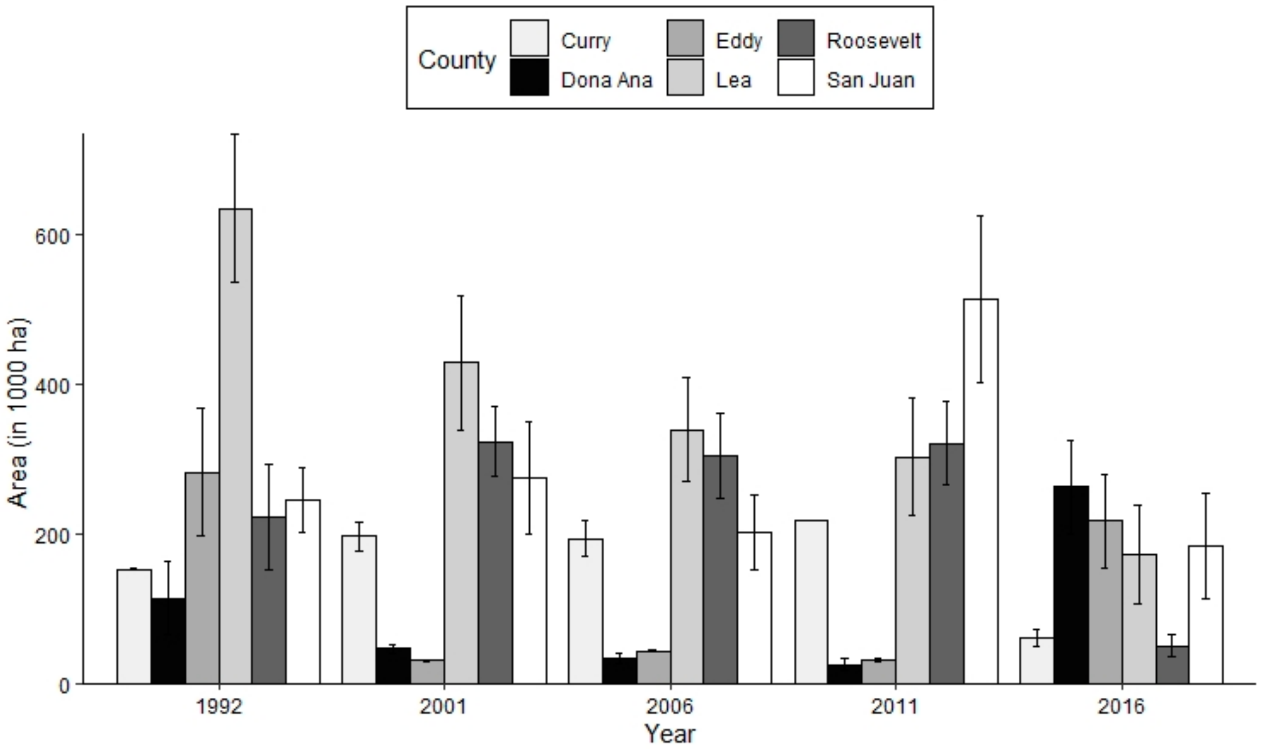
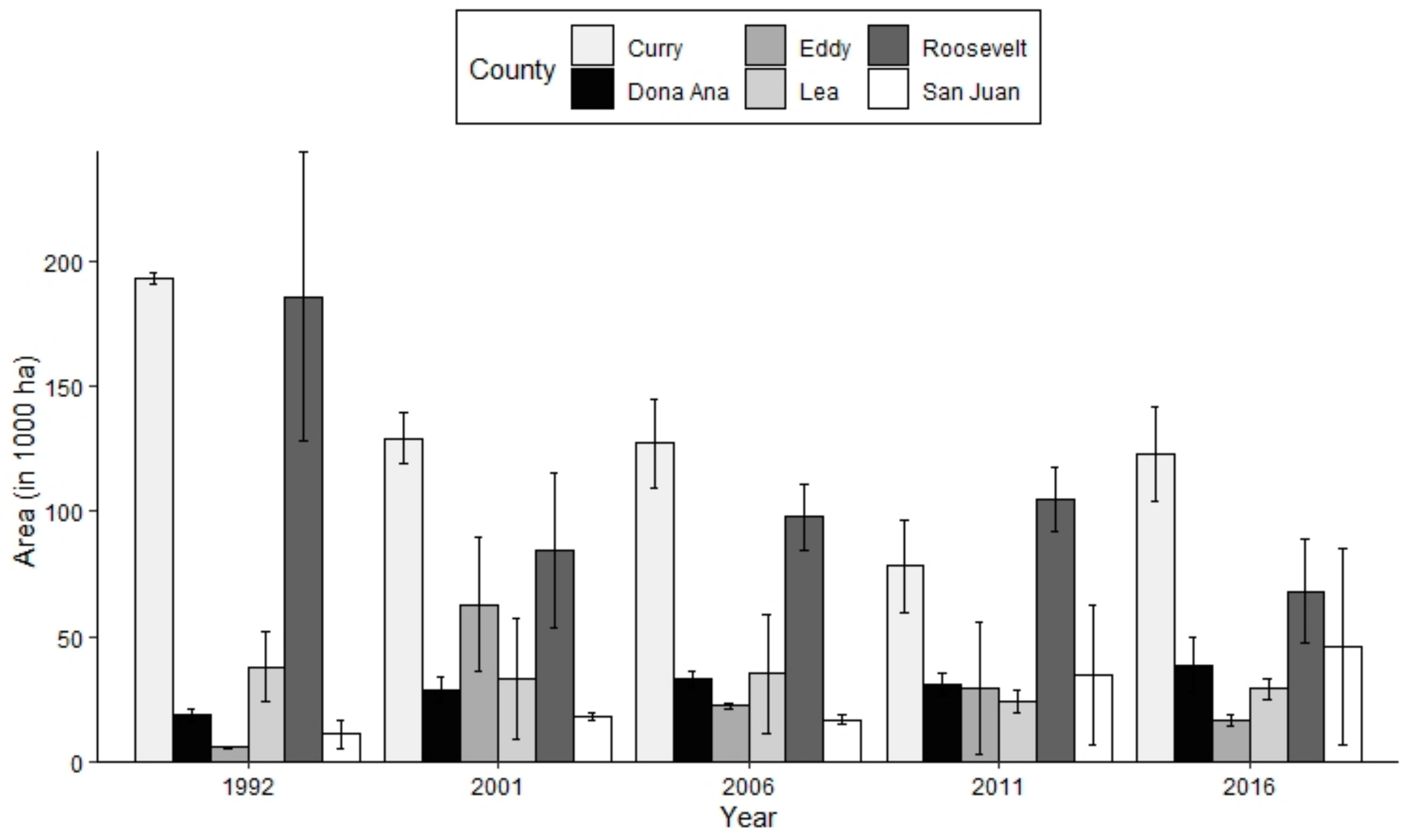
4.3. Area Estimation

The area estimates of the shrubland class over San Juan County showed a 31% decline during the 1992–2016 period (Figure 3). The total area of shrubland in San Juan county was the highest in 1992 with an estimated area of 1,018,761 ha and a Confidence Interval (CI) of ± 40,676 ha (or ±4%). In 2001, the shrubland area was about 754,619 ha ±18% showing a 26% decline compared to that of 1992. In 2006, there was ~5% increase in shrubland area (796,041 ha ±17%) compared to that of 2001 but indicated ~22% decline when compared to that of 1992. In 2011, shrubland area showed a 54% decline compared to that of 1992. In 2016, shrubland area was 704,024 ha ± 15% showed a 51% increase compared to that of the 2011 but indicated a 31% decline compared to that of 1992.
The shrubland area in Doña Ana showed an overall 10% net declining trend between 1992 and 2016. However, there was an increase in shrubland area during 1992–2001 followed by a consistent declining trend until 2016. The shrubland areas in Lea and Roosevelt counties showed a consistent increasing trend since 1992. The shrubland areas in 2016 in Lea and Roosevelt were about 860,008 ha ± 10% and 467,598 ha ± 8% indicating about 113% and 267% increase, respectively, compared to those in 1992. The shrubland area in Curry County was relatively very small (3367 ha ±2%) in 1992 and remained on average around 3000 ha until 2011, but in 2016 it showed a significant increase of about 146,638 ha ±7%. The shrubland area in Eddy county showed a 10% increase in 2016 (747,062 ha ±10%) compared to that of 1992 (680,065 ha ± 15%).
The grassland areas (Figure 4) in three counties including San Juan, Roosevelt, and Curry showed relatively similar behavior during the 1992–2016 period. The grassland areas in San Juan, Roosevelt, and Curry counties in 1992 of 245,741 ha ±17%, 222,360 ha ±32%, and 152,802 ha ±1%, respectively, showed 109%, 44%, and 43% increase between 1992 and 2011 followed by 64%, 84%, 72% decline between 2011 and 2016, respectively. In overall, the three counties (i.e., San Juan, Roosevelt, and Curry) showed declining trends of 25%, 77%, and 60% during the 1992–2016 period, respectively. On the contrary, a decreasing trend in grassland area was detected in Doña Ana County between 1992 and 2011 with total areas of 113,986 ha ±43% and 25,913 ha ±34%, respectively, indicating a ~77% decline. The overall behavior of grassland area in Doña Ana County indicated an increasing trend as the area in 2016 increased by about 130% compared to that of 1992. On the other hand, both Lea and Eddy counties showed consistent declining trends in grassland areas of about 73% and 23%, respectively, during the 1992–2016 period.
The cultivated cropland areas in Curry and Roosevelt counties in 1992 were the highest during the 1992–2016 period with 193,182 ha ±1% and 185,995 ha ±31%, respectively. In 2016, the areas in both counties dropped significantly by about 36% and 63%, respectively compared to those of 1992 (Figure 5). Similarly, in 2016, the cultivated cropland area in Lea County was about 29,082 ha ±14%, indicating a 24% decline compared to that of 1992 of 38,025 ha ±37%. The cultivated cropland areas in four counties including Lea, Eddy, San Juan, and Doña Ana were relatively lower (less than 50,000 ha on average) than those of Curry and Roosevelt. Three counties including Eddy, San Juan, and Doña Ana showed increasing trends during the 1992–2016 period. The cultivated cropland in Doña Ana County was 38,725 ha ±28% in 2016 indicating 100% increase compared to that of 1992 of 18,536 ha ±14%. Similarly, the Cultivated Crop areas in Eddy and San Juan in 2016 were about 16,682 ha ±16% and 45,754 ha ±86%, indicating about 180% and 300% increase compared to those of 1992, respectively.

5. Discussion

5.1. Accuracy Assessment

5.1.1. User’s Accuracy and Producer’s Accuracy

The results of user’s and producer’s accuracy of NLCD maps over the six counties showed a wide range of values. The user’s accuracy of the three main classes (i.e., shrubland, grassland, and cultivated cropland) were above 80%, 75%, and 80%, respectively when the NLCD maps from 1992 to 2016 were assessed using high-quality reference data but with few exceptions. Generally, it should be noted that there was no consensus on a specific accuracy threshold that can be considered as high or low. Rather, the decision of a high or low accuracy estimate can depend on the distribution, proportion, and size of the mapped classes [59]. Needless to say, the decision of categorizing an accuracy as high or low can also depend on mapping objectives, area being mapped, and distribution of the LULC classes. Therefore, based on the homogeneity and area proportions of the landscape and mapping product, different threshold of high (≥ 70%) and low (≤ 35%) accuracy estimates have been used in recent research findings [30]. Meaningful and useful accuracy estimates that can be achieved over heterogeneous area are usually low and respectively high accuracy estimates can be achieved over homogeneous regions when assessed with similar sampling designs [60]. In the assessment of NLCD maps over the six counties from 1992 to 2016, some instances were observed with relatively low accuracy (≤ 40%). For this analysis, a user’s or producer’s accuracy of ≥ 70% (≤ 40%) can be considered relatively high (low). It was also noticed that the obtained user’s accuracy values were relatively consistent compared to those of the producer’s accuracy.
The shrubland class showed some probability of occurrence of commission errors as depicted by moderate user’s accuracy values that ranged from 50%–62% in Table 5. The obtained user’s accuracy indicated that some pixels from other classes have been mapped or committed into the shrubland class (e.g., Roosevelt and San Juan counties in years 2001, 2011, and 2016). On the other hand, grassland class showed, in general, relatively low user’s accuracy that fell below 40%. For example, in Doña Ana County, the grassland class showed a user’s accuracy of 39% for in year 1992 (Table 5), indicating that there was more chance of occurrence of commission errors in grassland class compared to shrubland as well as cultivated cropland classes. In mapping the grassland class in this study, it was expected to obtain more commission errors or misclassification into this class generally due to spectral mixing with other classes, which is typical in naturally managed heterogenous regions. The user’s accuracy of cultivated cropland class did not fall below the lower threshold of 40% as observed in the other two classes (shrubland and grassland). The cultivated cropland class showed relatively higher accuracy than other classes because of its distribution and the homogeneity of this type of landscape in the study counties. Other studies also indicated that the misclassification of grassland and cultivated cropland is common and can be due to a number of reasons that include most importantly the timing of the Landsat images used to develop the most of the NLCD legacy maps [61]. The timing of some of the datasets of Landsat images used in developing NLCD is during early spring period (i.e., “leaf-off”). During such period (which may not be optimal to differentiate between some classes), there can be significant spectral similarities between grassland and cultivated cropland. Other factors that can affect and result in such misclassification include the way grasslands are managed (e.g., grazing practices), the phenology of grass species, and soil moisture conditions [61,62]. The three classes can be arranged from high to low in terms of chance of occurrence of commission errors or low to high user’s accuracy as grassland, shrubland, and cultivated cropland.
Additionally, the producer’s accuracy of the three main land cover classes (i.e., shrubland, grassland, and cultivated cropland) were above 70%, 80%, and 80%, respectively with few exceptions. The shrubland class of the NLCD maps showed high probability of occurrence of omission errors (i.e., omitted from shrubland to another class) with an estimated producer’s accuracy of 25% (Table 5) over Roosevelt county for year 1992. High probability of occurrence of omission errors (i.e., low producer’s accuracy with a range of 16%–22%) in cultivated cropland class was observed in San Juan and Eddy counties in 1992 and 2001, respectively. However, the grassland class did not show any low producer’s accuracy below 40% compared to those observed over shrubland and cultivated cropland classes (Table 5). With respect to the probability of omission errors, the three LULC classes can be arranged from high to low omission errors or from low to high producer’s accuracy as cultivated cropland, shrubland, and grassland, respectively. The relatively low producer’s accuracy that was observed over the cultivated cropland class can partly be attributed to small area proportion of this class and the low proportion of reference samples that were correctly classified on the map.

5.1.2. Overall Accuracy

The estimated OA showed a consistent pattern during the 1992–2016 period in most of the counties with few exceptions where a change in the accuracy can clearly be seen from one year to another over few counties. For example, the OA achieved 81% over Curry County in 2006, 73% over Doña Ana County in 1992, and 77% over Eddy County in 2006. The reason for this variability in the OA can partly be attributed to the differences between the classification algorithms that were used to develop the NLCD maps and the changes in the distribution and patterns of LULC classes in the respective counties. The OA in 1992 over Roosevelt County was about 71%, indicating the lowest value achieved across all counties during the1992–2016 period. Such low value can partly be attributed to the high chance of misclassification due to the low area proportion and distribution of LULC classes in this region, which can result in increased commission and omission errors. The highest OA of 100%, which was achieved over Curry County in 2011, can partly be explained by the dominance of the cultivated cropland class and the corresponding homogeneous nature of the land cover and the field sizes.
The estimated OA values over each county based on SEPAL were also compared with those of the NLCD maps as they were reported at regional and national scales (Table 7). It should be noted that the OA of the NLCD for 1992 was reported for six regions in the US that include the Pacific Northwest, Southwest, Rocky Mountains, Midwest, South Central, and Great Lakes for Anderson Level I and Level II. The South-central region included the state of New Mexico and therefore, the reported OA of this region were used and compared with those achieved using more robust region-specific assessment through the SEPAL tool. The OA values of the NLCD map of 1992 for the South Central region were about 74% and 44% for Anderson Level I and Level II, respectively [37,38]. The accuracy of the NLCD map of the South Central region reported for Anderson Level II was used to analyze the estimated OA of the six study counties in the year 1992. It was found that the estimated OA using SEPAL for the year 1992, were higher than those of the NLCD at the regional scale over all counties, except Curry County. The estimated OA for year 1992 based on SEPAL were more meaningful and representative at the county level as compared to the reported OA of 44% of the NLCD map for the South Central region.
Likewise, the estimated OA based on SEPAL was compared with the regional OA of the NLCD map of the year 2016 which was reported for different US regions and ranged between 71% and 97% [30]. It was noted that the OA of NLCD for the western US region ranged from 80% to upper 90%. An average value of 89% (based on the range of 80%–97%) was used in the analysis to be compared with those based on SEPAL. The reported OA of the NLCD maps of 2001, 2006, and 2011, at Anderson level II were 89%, 89% and 88%, respectively [39]. It was found that the estimated OA based on SEPAL of all the counties (i.e., 86%, 85%, and 82%) for these three years (i.e., 2001, 2006, and 2011) were relatively lower than the regional OA of the NLCD maps (Table 7).
The estimated OA in this study in each of the counties and years based on SEPAL showed complementary value with reference to those of the NLCD 1992–2016. This observation indicated that the related NLCD accuracies can be comparable over most of the study counties and may not be degraded from the reported regional ones. At the same time, the estimated OA based on SEPAL also provided more insights about the need to perform consistent assessment of the NLCD maps at county level.

5.2. Area Estimation and Observed Trends

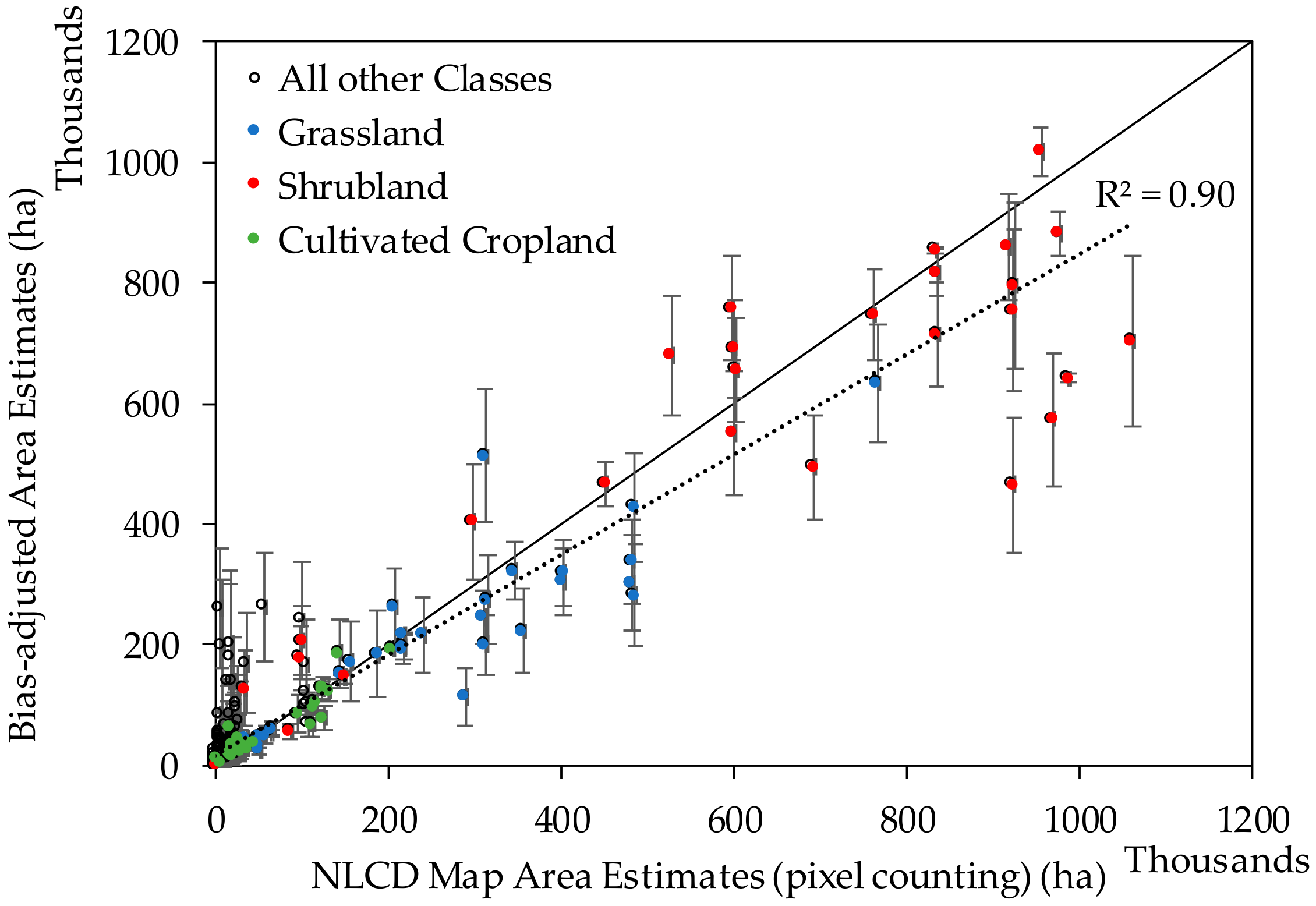
5.2.1. Bias-Adjusted and Pixel Counting Area Estimates

The methods of estimating areas of mapped classes have been discussed in a number of recent studies (e.g., [63,64,65,66]). However, the estimation methods still have some degree of uncertainty (rather a lack of identifying a common approach) when it comes to determine the true area proportions on the ground. In order to account for the uncertainty in area estimation of mapped and change classes, standard error or estimators can provide adjusted change area with confidence intervals. A recent review by [66] provided an assessment of approaches used to estimate bias-adjusted areas and associated accuracies of NLCD maps. Based on this review by [66], it appeared that out of the 57 publications identified in two remote sensing journals, only nine studies provided the accuracy measures and the information needed to compute the bias-adjusted area estimates. It is evident that even with high levels of accuracy area estimates obtained directly from a map (i.e., pixel counting), which is common used, can provide biased area estimates due to classification errors that need to be adjusted for as suggested by [66]. The findings from this analysis provided similar indications about the differences (i.e., discrepancies) between the use of pixel counting and bias-adjusted area estimates based on stratified area estimator (Figure 6).
A comparison between the bias-adjusted and the NLCD map (i.e., pixel counting) area estimates for all classes including those for grassland, shrubland, and cultivated cropland is shown in Figure 6. The comparison showed mixed indications of discrepancies. However, it appeared that the majority of bias-adjusted area estimates were lower than those obtained directly from the NLCD map area (i.e., pixel counting). In other words, area estimates based on pixel counting overestimated the bias-adjusted ones. This finding is relatively similar to that of [66] in which they obtained some mixed indications of discrepancies when comparing area estimates based on pixel counting and a stratified estimator. This comparison also showed that there was a variable degree of uncertainty across all LULC classes as represented by the estimated margin of error as indicated by the 95% CI. It should be noted that this margin of error can only be estimated for the bias-adjusted area estimates. The shrubland class showed high uncertainty (a wide range of the 95% CI) in area estimation partly due to relatively higher misclassification errors as compared to other classes. Generally, area estimates based on pixel counting do not match with the true proportion areas of the ground.
Moreover, in this analysis, area estimates based on pixel counting were generated at spatial resolution, temporal resolution, and/or classification schemes that are different from those that can be obtained from other existing mapping products such as the GAP Analysis Program (GAP) and Cropland Data Layer (CDL) [61,67]. Thus, limited the ability to provide reasonable comparisons [68,69] that can be help in further evaluating the obtained area estimates. This study further highlighted the need to provide accurate bias-adjusted area estimates compared to using pixel counting approach that is commonly used in literature.

5.2.2. Class Specific Area Estimates Uncertainty

The estimated shrubland areas over some counties exhibited relatively high levels of uncertainty as indicated by the corresponding CI values. These high uncertainties can mostly be attributed to high commission errors. In some instances, the relatively high uncertainty (i.e., based on the obtained 95% CI) of grassland area estimates in Lea County (2006) was associated with commission error from shrubland cover (22%), developed (2.2%), and cultivated cropland covers (2.2%) (Table A7). The CI over Eddy County in 2011 showed uncertainty in shrubland class areas due to high commission error from barren land (39%) and forest (10%) classes (Table A8). Likewise, over Doña Ana County in 1992, 5% of Developed class was classified as shrubland (Table A9). Similarly, 8% of barren land and 3% of grassland classes in Curry County in (2006) were classified as shrubland (Table A10). The uncertainty in grassland and shrubland class might be due to spectral mixing of these classes with the developed class (e.g., oil and natural gas pads) and contribute to errors in the classification process.
Generally, the high uncertainty in grassland area estimates during 2011 can partly be attributed to increased water stress conditions in NM’s rangelands due to frequent and persistent drought events since 2000 as well as increased temperature anomalies since 1990 (Figure 7) [19]. These conditions can result in reduced spectral signature differences (i.e., similar spectral features) between grassland and other adjacent Earth’s features or classes (e.g., cultivated crops and shrubland). Such similarities can consequently contribute to the omission of grassland pixels from true classification, and its commission to the shrubland such as those observed in San Juan in 2011 (Table A11).
Moreover, cultivated cropland area estimates over Eddy County in year 2001 and 2011 showed relatively high values of CI. Misclassification of shrubland (9%) pixels in the NLCD 2011 was detected in Eddy County (Table A8). This can also be partly explained by the persistent and frequent drought events during the study period, which can affect vegetation growth and result in spectral similarities between land cover classes (i.e., particularly grassland and shrubland) and cultivated cropland. The study showed that most of the uncertainty values of the area estimates appeared to be from misclassification among shrubland, grassland, cultivated cropland, and forest pixels.

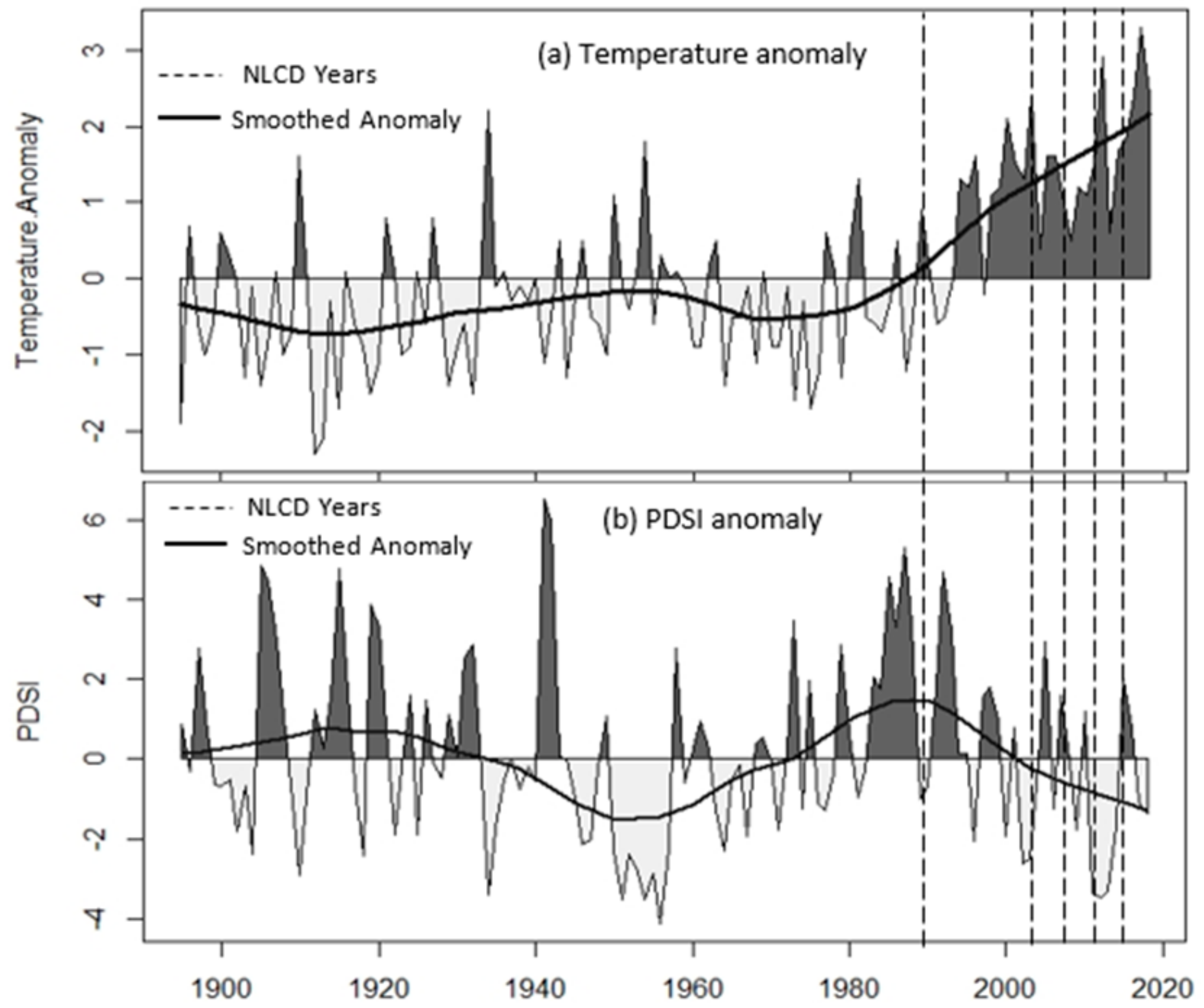
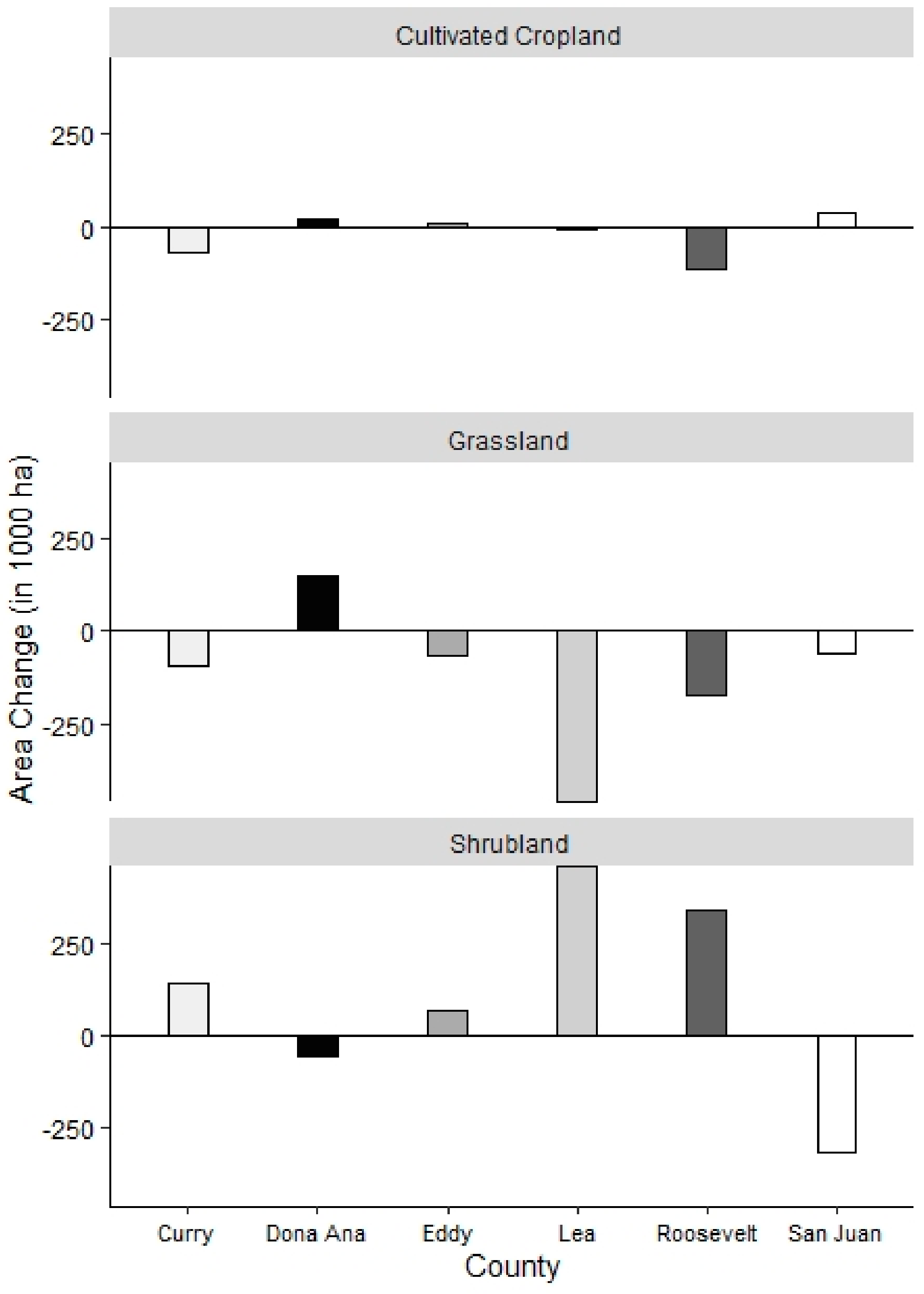
5.2.3. Observed Trends

This part of the analysis was aimed to present preliminary indications and highlight potential connections between observed LULC area changes and climate variables over New Mexico that can be used to guide ongoing and future analysis as part of modeling efforts of NM’s FEWS Nexus led by authors as shown in [20,22,23]. A summary of the net area changes of grassland, shrubland, and cultivated cropland between 1992 and 2016 over each county is shown in Figure 8. The observed LULC change behavior suggested that shrubland experienced a net increasing trend in four counties that all lie in southeast NM and net declining trends in Doña Ana (southcentral NM) and San Juan (northwest NM) counties. Out of these four counties, the increase in shrubland areas over Lea and Roosevelt counties was significant compared to those over Curry and Eddy counties. On the other hand, grassland areas experienced a net decreasing trend in five counties and a net increasing trend in Doña Ana County. A subtle decline in grassland areas was observed in Lea County, followed by Roosevelt County, with a relatively similar declining trend in the rest of the counties (i.e., Curry, Eddy, and San Juan). The observed trend in Doña Ana County indicated a decline in shrubland and an increase in grassland. Similarly, the observed trend in San Juan County indicated declining trends in both shrubland and grassland areas. Interestingly, the four counties that showed a net increasing trend in shrubland areas (i.e., Curry Roosevelt, Lea, and Eddy) simultaneously showed almost relatively similar declining trends (i.e., amount of area change) in grassland areas. A number of reasons can partly explain this observation. The decrease in the extent of grassland can be partially attributed to the encroachment of shrubland in the expense of the grassland, particularly where the counties showed net increase in shrubland cover (Figure 8). However, it should be noted that this study was focused on the changes in area estimates but not the dynamic nature of the changes. Thus, it was not readily clear in this study if the reduction in grassland class areas was directly due to shift in land cover to shrubland. Additional analysis will be conducted to evaluate dynamic LULC change.
Some recent studies similarly suggested that the encroachment of shrubland was in the expense of grassland, especially in the western US, including for example those by [19,70]. As the study by [70] was conducted at the conterminous US (CONUS) scale during 2001–2016 using NLCD data, it indicated that both grassland and shrubland increased in areas with regionally variable amounts of change. The findings in [70] suggested the increase in shrubland areas was at the expense of forest loss and grassland change to shrubland and the increase in grassland areas was at the expense of forest and shrubland losses. Moreover, the study by [19] suggested there was an increased level of encroachment of woody vegetation (in which shrubland can be considered as one of its subclasses) in NM’s rangelands, which is dominantly covered by grasslands. The study by [19] was based on land cover analysis using Landsat data for the period 1984–2017 as explained in the Rangeland Analysis Platform (RAP) [71,72]. Woody plant encroachment was also suggested as one of the reasons of declining grassland areas as indicated by [73] due to lack of precipitation, fire disturbances, over grazing, and its association with rising level of CO2 in the atmosphere which can favor the growth of C3 woody vegetation.
The declining trend in grassland areas was consistent with the increased temperature anomaly over NM and was also associated with a decline in grassland productivity in the state as indicated in [17]. This observation highlights the importance and need to assess the extent and quality of rangelands components (i.e., grasslands and shrublands) as they play significant role in NM’s food production systems [20,74]. The study by [6] also suggested that the loss of rangeland ecosystems was due to crude oil and natural gas activities. However, the study by [6] didn’t provide a distinction between grassland and shrubland classes to evaluate the effect of each land cover type on the other.
Only three counties showed significant area change in cultivated cropland that included Doña Ana, Curry, and Roosevelt. The cultivated cropland area in Doña Ana County showed a significant increasing trend during the 1992–2016 period. On the contrary, the cultivated cropland area Curry County consistently decreased in during 1992–2016, though there was an increase between 2011 and 2016. The cultivated cropland area consistently decreased over Roosevelt. In the rest of the counties (i.e. Eddy, Lea, and San Juan), the cultivated cropland area estimates showed a net increase in Eddy and San Juan counties and a net decrease over Lea County.
It was observed that the net decrease in the cultivated cropland areas in the study counties was associated with an increasing temperature anomaly that started since the 1990s as well as frequent and persistent drought events [19] (Figure 7). Moreover, the counties that experienced net declining trends (i.e., Curry, Lea, Roosevelt) are located in areas (southeast New Mexico) with limited to no surface water supplies—a condition that makes these counties rely heavily on groundwater resources (for irrigation) that also showed a declining trend in water levels in recent years [75,76]. Another potential reason for the net decreasing trend in cultivated cropland in the three counties in eastern NM can be attributed to the expansion of Barren Land cover, mostly due to increased fragmentation of the land due to crude oil and natural gas drilling activities (production pads). The recent finding by [6] that was conducted during the period between 2000 and 2012 indicated that the loss of ecosystem services including cropland in North America was directly associated crude oil and natural gas activities. The net increasing trend in the other three counties, including Doña Ana, San Juan, and Eddy, can partly be explained by the fact that most of the cropland areas in these counties are located in regions that rely on surface water resources (near river corridors) or conjunctive use of surface and groundwater sources, specifically the Lower Rio Grande, San Juan, and Pecos rivers, respectively.

6. LULC Change and FEWS: A Perspective

Most of the recent research findings of area estimation applications were based and performed at regional and large scales and different scopes (mainly over cropland and forest covers). For example, there were many applications related to land cover change (e.g., [44]), land use mapping and monitoring (e.g., [77]), biomass estimation (e.g., [78]), forest disturbance and change in forest types [79], and estimating cultivated cropland area and abandonment (e.g., [80,81]). However, there is a lack of studies related to providing more accurate (bias-adjusted), consistent, and long time series area estimates (e.g., compared to the single time estimates by [82]) that can be used to evaluate, quantify, and manage FEWS land resources especially at county scale. Thus, this study was conducted partly to highlight the importance of addressing this issue. The LULC bias-adjusted area estimates and their uncertainties at county level can particularly be helpful in developing an improved characterization of the interconnected FEWS components. Therefore, extending the usability of operational products, such as the NLCD at such scale, allows for a more appropriate evaluation of FEWS behavior in responses to (consistent and highly accurate estimates of) LULC area changes.
In this study, the focus was on land resources that support NM’s food production systems including rangeland components (i.e. grassland and shrubland) and cultivated cropland classes because of their environmental and socioeconomic importance for functionally sustainable NM’s FEWS [19,20,21,22,74]. Generally, FEWS nexus decisions require addressing complex natural resource and development challenges for an improved sustainability [22,23]. Thus, the knowledge about the extent and land area change estimates consequently has great role in evaluating the behavior of FEWS that can in turn reflect their response to changing environmental and climate conditions, such as rising temperatures, heat waves, variable precipitation, and severe and persistent drought among others. All these changes can directly affect rangeland and cropland availability and productivity as they support livestock and crop production. In particular, as ~92% of NM’s land can be considered as rangeland [16], recent studies from NM and southwest US suggested that rangeland carrying capacity may have been reduced by as much as 30% due to climate change [17,19]. A summary of the observed relative LULC area change over the six counties between 1992 and 2016 (Table 8) indicated reduced grassland areas where it was needed the most, potentially due to encroachment from woody vegetation (shrubs); increased shrubland area over the same counties that experienced decrease in grasslands; and; and reduced cropland areas in region with increased reliance on groundwater for irrigation. Hence, this depiction of the changes in LULC highlighted the need for consistent and reliable land resource information, which can help in accurately monitoring available natural resources and develop an improved understating of the NM’s FEWS as well as sustainable management practices.

7. Limitations and Future Work

As the study was aimed at providing more accurate estimates of LULC area over the main three classes that include shrubland, grassland, and cultivate cropland that can be used to provide an improved understanding and characterization of NM’s FEWS county level, the authors acknowledged some limitations that need to be considered when using the obtained findings. Generally, the SEPAL and the other tools used provided an effective means to conduct this analysis. However, the reference data collection involved using automatically generated reference samples. These reference samples were then labeled following a visual inspection of satellite imagery in Google Earth using the Collect Earth tool. The reference samples that were labeled with a low confidence (e.g., located on the edges of land cover classes) were expected to be manually dropped (removed) by the interpreter rather than reallocating them to more well-defined surfaces. This process (i.e., dropping of samples) could result in a lower sample size for each selected region. Considering the large number of reference samples collected in this analysis the authors made sure to follow the guidelines related to minimum number of sample as explained in [44]. Moreover, the bias-adjusted area estimates were only compared with pixel counting estimates because of the limited data availability such as true area proportions of land cover classes or high spatial resolution remote sensing thematic maps at county level.
To address some of these limitations the authors will compare the obtained area estimates with other dataset that have similar characteristics as it becomes available. One of the datasets include the Crop Data Layer [69], which currently has limited data over New Mexico that only go back to 2006. Additionally, the authors are planning to make use of the new generation of NLCD [30] that has relatively higher temporal resolution (every two years) for a more consistent bias-adjusted area estimates. Dynamic LULC change will be conducted to evaluate how each LULC class is shifting and affecting other classes. This can be helpful in determining for example the loss of natural ecosystems to Developed and/or encroachment of woody vegetation (shrubland) in grassland. Moreover, additional analysis will be conducted in the future to cover all NM’s counties in New Mexico.

8. Conclusions

The main goal of the study was to examine the usability of the single-date NLCD legacy maps (i.e., 1992, 2001, 2006, 2011, and 2016) at the county level decisions to help in resource monitoring, management, and conservation in New Mexico as well as other areas with similar semi-arid conditions. This research highlighted some of the uncertainties related with the use of NLCD area estimates over a few LULC classes (i.e., grassland, shrubland, and cultivated cropland) that mostly contribute to NM’s FEWS in six counties that include San Juan, Curry, Roosevelt, Lea, Eddy, and Doña Ana. The cloud-based computation and analysis tools in SEPAL provided standardized and consistent sample allocation, integrate appropriate response design, and analysis of area estimates and uncertainties. These characteristics in SEPAL allowed for efficient application and evaluation of LULC change trends at the county level. This is important, especially in southwest US region where it can be challenging to obtain highly accurate estimates of LULC area change. The producer’s and user’s accuracies over some of the three LULC classes showed wide ranges of accuracy levels. Based on SEPAL, the obtained OA of the NLCD maps at the county level during the 1992–2016 period ranged from 71%–100%, and were lower compared to those of the NLCD maps at the regional and national scales. The commission errors mostly emanated from intermixing and spectral similarity between some of the LULC classes. For example, the commission of pixels from one class to the other was evident between shrubland and grassland; cultivated cropland and shrubland; and grassland and Forest. The shrubland cover showed a net area increase in all the study counties except in Doña Ana and San Juan counties. On the contrary, grassland showed a decreasing trend in all the study counties except in Doña Ana. Cultivated cropland, in general, exhibited decreasing trends in three counties (i.e. Curry, Roosevelt, and Lea) and increasing trends in the rest of the counties. The LULC area estimates obtained at the county level based on SEPAL were generally lower than those obtained directly from NLCD maps (pixel counting).
In recent years, cloud computing approaches using different platforms, such as GEE, Amazon Web Services (AWS), and Open Foris among others are emerging as powerful means to efficiently process large datasets and reduce the need for massive local storage and computational requirements. Likewise, the SEPAL platform, which is also publicly accessible, integrates a number of existing tools to facilitate and specifically enhance land monitoring. Some of the main advantages of SEPAL include its ability to:
  • Provide standardized, robust, and semi-automated protocols for LULC accuracy assessment, and uncertainty analysis.
  • Allow the comparison of multitemporal land cover data of the same location at local and national mapping scales by facilitating access to several remote sensing data sources
  • Conserves storage and computational resources needs by providing and integrating inbuilt access to other cloud-based platforms as well as data sources.
  • Provide improved computational efficiency and it is easily adaptable, as it requires minimal local computing capacities and human resources.
The findings of this study can help in developing an improved understanding about the behavior of NM’s FEWS; assess their corresponding response to environmental and climatic changes; and provide guidance to develop management practices to enhance the sustainability of NM’s natural resources. However, further studies are still needed to provide a time series of area change estimates at high spatial resolution. For example, by using the new generation of NLCD maps; detect the dynamic changes of the ecosystem structure; and evaluate their relationship with essential climate variable such as temperature and precipitation particularly over shrublands and grassland (i.e., rangeland ecosystems) as they play a great role in NM’s food production systems. While this study was conducted over New Mexico, its findings can be extended to other regions with similar conditions.

Author Contributions

Conceptualization, H.M.E.G.; Data curation, M.G.G. and A.J.Z.; Formal analysis, M.G.G.; Funding acquisition, H.M.E.G.; Investigation, M.G.G. and H.M.E.G.; Methodology, M.G.G. and H.M.E.G.; Project administration, H.M.E.G.; Resources, H.M.E.G.; Software, M.G.G. and Y.F.; Supervision, H.M.E.G. and K.Y.; Validation, M.G.G., H.M.E.G. and K.Y.; Visualization, M.G.G., H.M.E.G. and K.Y.; Writing—original draft, M.G.G.; Writing—review & editing, H.M.E.G., K.Y. and K.G.B. All authors have read and agreed to the published version of the manuscript.

Funding

This research was partially funded by the National Science Foundation (NSF), awards #1739835 and #IIA-1301346, and New Mexico State University.

Acknowledgments

The authors would like to thank the National Forest Monitoring (NFM) Team REDD+/NFM cluster, Forestry Department Food and Agriculture Organization (FAO) of the United Nations for their support in the use of SEPAL and the cloud based computational infrastructure.

Conflicts of Interest

The authors declare no conflict of interest. The funders had no role in the design of the study; in the collection, analyses, or interpretation of data; in the writing of the manuscript, or in the decision to publish the results. Any opinions, findings, and conclusions or recommendations expressed in this material are those of the author(s) and do not necessarily reflect the views of the National Science Foundation.

Appendix A

A description of the LULC classes used for reference data collection, labeling, and area estimation.
Table A1. Description of LULC classes. The text and numbers in bold highlight the name and code of THE LULC classes used in the study.
Level 1 Level IILULC Classes Description
Water Open Water (11)
Perennial Ice/Snow (12)
(11) Areas of open water, generally with less than 25% cover of vegetation or soil. (12) Areas characterized by a perennial cover of ice and/or snow, generally greater than 25% of total cover.
DevelopedOpen Space (21)
Low Intensity (22)
Medium Intensity (23)
High Intensity (24)
(21) Areas with a mixture of constructed materials, but mostly vegetation in the form of lawn grasses with 20% impervious surfaces (e.g., large-lot single-family housing units, parks, and golf courses). (22) Areas with a mixture of constructed materials and vegetation. Impervious surfaces account for 20% to 49% percent of total cover (e.g., single-family housing units), (23) like (22) but with 50% to 79% of impervious surfaces. (24) Highly developed areas (e.g., apartment complexes, row houses, and commercial/industrial) with 80% to 100% impervious surfaces.
BarrenBarren Land (31) (Rock/Sand/Clay)Areas of bedrock, desert pavement, scarps, talus, slides, volcanic material, glacial debris, sand dunes, strip mines, gravel pits and other accumulations of earthen material. Generally, vegetation accounts for less than 15% of total cover.
ForestDeciduous Forest (41)
Evergreen Forest (42)
Mixed Forest (43)
(41) Areas dominated by trees generally greater than 5 meters tall, and > 20% of total vegetation cover with more than 75% of the tree species shed foliage simultaneously in response to seasonal change. (42) Areas with more than 75% of the tree species maintain their leaves all year and canopy never without green foliage. (43) Area with more than 75% of the tree species maintain their leaves all year and neither deciduous nor evergreen species are greater than 75% of total tree cover.
shrublandDwarf Scrub (51)
Shrub/Scrub (52)
[or shrubland]
(51) Areas dominated by shrubs; less than 5 meters tall with shrub canopy typically greater than 20% of total vegetation. (52) This class includes true shrubs, young trees in an early successional stage or trees stunted from environmental conditions.
grasslandgrassland/ Herbaceous (71)
Sedge/Herbaceous (72)
Lichens (73)
Moss (74)
(71) Areas dominated by graminoid or herbaceous vegetation, generally greater than 80% of total vegetation. These areas are not subject to intensive management, such as tilling but can be utilized for grazing. (72), (73), and (74) are Alaska only classes.
Planted/ CultivatedPasture/ Hay (81)
Cultivated Crops (82)
(81) Areas of grasses, legumes, or grass-legume mixtures planted for livestock grazing or the production of seed or hay crops, typically on a perennial cycle. (82) Areas used to produce annual crops, such as corn, soybeans, vegetables, tobacco, and cotton, and perennial woody crops such as orchards and vineyards. This class also includes all land being actively tilled
WetlandsWoody Wetlands (90)
Emergent Herbaceous Wetlands (95)
(90) Areas where forest or shrubland vegetation accounts for greater than 20% of vegetative cover and the soil or substrate is periodically saturated with or covered with water.
(95) Areas where perennial herbaceous vegetation accounts for greater than 80% of vegetative cover and the soil or substrate is periodically saturated with or covered with water.

Appendix B

A summary of the obtained user’s accuracy and producer’s accuracy over the rest of the LULC classes.
Table A2. User’s and producer’s accuracy for the rest of the LULC classes for the NLCD map of 1992.
County1992
AccuracyWBDEVBRLFRLPSLWWEHW
CurryPA573052 100
UA10010083 82
Doña AnaPA81100202072097
UA8282958448080
EddyPA 10045359816100
UA 759796889548
LeaPA99119810074100100
UA10086605854444
RooseveltPA 9885100100
UA 71521483
San JuanPA1009126100 1498
UA91868564 3252
WB = Water body, DEV = Developed, BRL= Barren land, FRL = Forest Land PSL= pasture/hay, WW= Woody Wetland, and EHW= Emergent Herbaceous Wetlands.
Table A3. User’s and producer’s accuracy for the rest of the LULC classes for the NLCD map of 2001.
County2001
AccuracyWBDEVBRLFRLPSLWWEHW
CurryPA825450 100
UA889987 100
Doña AnaPA2644100661374
UA779183927510085
EddyPA77391993 2147
UA92967393 8070
LeaPA7694810 43100
UA10078630 8953
RooseveltPA95208 09
UA969744 092
San JuanPA953037889610026
UA8685100100817085
The description of the different columns and row is same as in Table A2.
Table A4. User’s and producer’s accuracy for the rest of the LULC classes for the NLCD map of 2006.
County2006
AccuracyWBDEVBRLFRLPSLWWEHW
CurryPA886525696 3
UA7686956772 89
Doña AnaPA96979496262061
UA85879792758120
EddyPA7610426095
UA71906461559653
RooseveltPA881004100 10097
UA1008291100 6739
San JuanPA9290100628799100
UA958896100855978
LeaPA5926570 47100
UA10078720 10070
The description of the different columns and row is same as in Table A2.
Table A5. User’s and producer’s accuracy for the rest of the LULC classes for the NLCD map of 2011.
County2011
AccuracyWBDEVBRLFRLPSLWWEHW
CurryPA349111 162
UA1009575100 8858
Doña AnaPA1004721991699100
UA888410084667650
EddyPA749122731012
UA88908899739277
RooseveltPA1004780100 5987
UA91868564 3252
San JuanPA151547100171850
UA91947492798092
LeaPA634075100 7216
UA92818176 10048
The description of the different columns and row is same as in Table A1.
Table A6. User’s and producer’s accuracy for the rest of the LULC classes for the NLCD map of 2016.
County2016
AccuracyWBDEVBRLFRLPSLWWEHW
CurryPA85801 100099
UA889684 10010082
Doña AnaPA9921502401
UA8982769210095
EddyPA96962133 4396
UA98678088 9285
RooseveltPA90276 2010016
UA969383 804863
San JuanPA8986438952285
UA97829393838837
LeaPA933054 10069100
UA887872 1008472
The description of the different columns and row is same as in Table A2.

Appendix C

Some of the estimated error matrixes for select counties and years were shown here to support the findings of this analysis. The reported errors were expressed as percent of area weighted by samples in agreement or disagreements by the total samples. The Standard Error (SE) is stratified estimator of proportion areas, the Area Estimates (AE) is adjusted area estimates which was obtained by subtracting the area of commissioned area (ha) from area of map data (before adjustment) and adding omitted area (ha).
Table A7. Error matrix of Lea County (2006) expressed by Area Weighted Proportions (%).
Reference Data (2006)
Map1120315271829095UA
Map data (2006)11960000000100
20033332140078
3196566000072
5205083000094
71020226220070
82033100800082
900000001000100
95000015.01.57070
WPA (%)59265782996545100
AE (ha)127264,3135,476692,112338,70735,25898242
SE (ha)28626,8251,16041,15735,39712,2222836
95% CI (ha)56052,5762,27380,66869,37923,9565671
SE = Standard Error, CI = Confidence Interval, WPA = Weighted Producer’s Accuracy, UA = User’s Accuracy. Land cover classes codes: Open Water (11), Developed (20), Barren Land (31), Forest (40), shrubland (52), grassland (71), cultivated cropland (82), Woody Wetland (90), and Emergent Herbaceous Wetland (95).
Table A8. Error matrix of Eddy county (2011) expressed by Area Weighted Proportions (%).
Reference Data (2011)
Map 1120314052718182UA
Map data (2011)1182082000088
2089530000090
3106550200088
4001079000099
520039108800259
71002621000091
81000350095073
8203309008886
WPA (%)74915527100100354
AE (ha)547416,666259,89294,486574,18331,35410526,391
SE (ha)46483650,19728,91556287140310113,342
95% CI (ha)910163998,38656,674110,322275019926151
The description of the different columns and row is same as in Table A7.
Table A9. Error matrix of Doña Ana County (1992) expressed by Area Weighted Proportions (%).
Reference Data (1992)
Map112031527182UA
Map data (1992)11960 0 0 0 0 100
200 3.4293320478
3196.35660 0 72
520 50 820 0 94
710 2.20 2262270
820 333100 8083
WPA(%)59265710010065
AE (ha)127264,3135476692,11233,870735,258
SE (ha)28626,82511,56041,15735,397.212,222
95% CI (ha)559.752,576.32272.580,66869,37923,956
The description of the different columns and row is same as in Table A7.
Table A10. Error matrix of Curry County (2006) expressed by Area Weighted Proportions (%).
Reference Data (2006)
Map1120315271829095UA
Map Data (2006)11820530016088
20099100100065
313062000002
52008973006100
7102208302098
820110100091
9020005980096
9550100191403
WPA (%)88656256100989140
AE (ha)18624,07010,4913,326193,468127,438485618
SE (ha)186179617418211,874903245436
95% CI (ha)3512,11112,10035723,27217,703710,654
The description of the different columns and row is same as in Table A7.
Table A11. Error matrix of San Juan county (2011) expressed by Area Weighted Proportions (%).
Reference (2011)
Map1120314052718182UA
Map Data (2011)1115010000091
2001500000094
3129470222074
40030100300092
523243099546350
7130000518083
8100000017479
8202000005089
900100001080
950200002092
WPA(%)15154710099511750
AE (ha)32,403139,01226,83297,464465,505512,88182,27034,637
SE (ha)19,11937,50314,070329557,36656,53229,18814,128
95%CI (ha)37,47373,50627,5786458112,438110,80257,20927,691
The description of the different columns and row is same as in Table A7.

References

  1. U.S. Global Change Research Program Fourth National Climate Assessment. Available online: https://nca2018.globalchange.gov/downloads/ (accessed on 16 October 2019).
  2. Karabulut, A.; Egoh, B.N.; Lanzanova, D.; Grizzetti, B.; Bidoglio, G.; Pagliero, L.; Bouraoui, F.; Aloe, A.; Reynaud, A.; Maes, J.; et al. Mapping water provisioning services to support the ecosystem–water–food–energy nexus in the Danube river basin. Ecosyst. Serv. 2016, 17, 278–292. [Google Scholar] [CrossRef]
  3. Flammini, A.; Puri, M.; Pluschke, L.; Dubois, O. Walking the Nexus Talk: Assessing the Water-Energy-Food Nexus in the Context of the Sustainable Energy For All Initiative. In Environment and Natural Resources Management Working Paper; Climate, Energy and Tenure Division (NRC), Food and Agriculture Organization of the United Nations: Rome, Italy, 2014; ISBN 978-92-5-108487-8. [Google Scholar]
  4. Zhu, Z.; Woodcock, C.E.; Olofsson, P. Continuous monitoring of forest disturbance using all available Landsat imagery. Remote Sens. Environ. 2012, 122, 75–91. [Google Scholar] [CrossRef]
  5. Ramankutty, N.; Evan, A.T.; Monfreda, C.; Foley, J.A. Farming the planet: 1. Geographic distribution of global agricultural lands in the year 2000: GLOBAL AGRICULTURAL LANDS IN 2000. Glob. Biogeochem. Cycles 2008, 22, 1–19. [Google Scholar] [CrossRef]
  6. Allred, B.W.; Smith, W.K.; Twidwell, D.; Haggerty, J.H.; Running, S.W.; Naugle, D.E.; Fuhlendorf, S.D. Ecosystem services lost to oil and gas in North America. Science 2015, 348, 401–402. [Google Scholar] [CrossRef] [PubMed] [Green Version]
  7. IPCC (2) (PDF) Completion of the 2006 National Land Cover Database for the Conterminous United States. Available online: https://www.researchgate.net/publication/279868428_Completion_of_the_2006_National_Land_Cover_Database_for_the_Conterminous_United_States (accessed on 30 October 2019).
  8. Tilman, D. Forecasting Agriculturally Driven Global Environmental Change. Science 2001, 292, 281–284. [Google Scholar] [CrossRef] [PubMed] [Green Version]
  9. Ramankutty, N.; Foley, J.A. Estimating historical changes in global land cover: Croplands from 1700 to 1992. Glob. Biogeochem. Cycles 1999, 13, 997–1027. [Google Scholar] [CrossRef]
  10. Lambin, E.F.; Meyfroidt, P. Global land use change, economic globalization, and the looming land scarcity. Proc. Natl. Acad. Sci. USA 2011, 108, 3465–3472. [Google Scholar] [CrossRef] [Green Version]
  11. Dale, V.H.; Efroymson, R.A.; Kline, K.L. The land use–climate change–energy nexus. Landsc. Ecol. 2011, 26, 755–773. [Google Scholar] [CrossRef]
  12. Loveland, T.R.; Sohl, T.L.; Stehman, S.V.; Gallant, A.L.; Sayler, K.L.; Napton, D.E. A Strategy for Estimating the Rates of Recent United States Land Cover Changes. Photogramm. Eng. 2002, 68, 1091–1099. [Google Scholar]
  13. Webb, J. Image-based Change Estimation for Land Cover and Land Use Monitoring. In Moving from Status to Trends: Forest Inventory and Analysis Symposium 2012; CreateSpace Independent Publishing Platform: Scotts Valley, CA, USA, 2015; pp. 46–53. [Google Scholar]
  14. Gonzalez, P.G.M.; Garfin, D.D.; Breshears, K.M.; Brooks, H.E.; Brown, E.H.; Elias, A.; Gunasekara, N.; Huntly, J.K.; Maldonado, N.J.; Mantua, H.G.; et al. Impacts, Risks, and Adaptation in the United States: Fourth National Climate Assessment; Reidmiller, D.R.C.W., Avery, D.R., Easterling, K.E., Kunkel, K.L.M., Lewis, T.K., Maycock Stewart, B.C., Eds.; U.S. Global Change Research Program: Washington, DC, USA, 2018; Volume 2, pp. 1101–1184.
  15. WRI (World Resources Insatiate). Aqueduct Water Risk Atlas. Available online: https://www.wri.org/resources/maps/aqueduct-water-risk-atlas (accessed on 4 January 2020).
  16. Allison, R.C.D.; Ashcroft, N. New Mexico Range Plants; New Mexico State University Cooperative Extension Service and Agricultural Experiment Station Publications: Las Cruces, NM, USA, 2011; p. 48. [Google Scholar]
  17. McIntosh, M.; Holechek, J.L.; Spiegal, S.; Cibils, A.F.; Estell, R. Long term declining trends in Chihuahuan Desert forage production in relation to precipitation and ambient temperature. Rangel. Ecol. 2019, 72, 976–987. [Google Scholar] [CrossRef]
  18. Zaied, A.J.; Geli, H.M.E.; Holechek, J.L.; Cibils, A.F.; Sawalhah, M.N.; Gard, C.C. An Evaluation of Historical Trends in New Mexico Beef Cattle Production in Relation to Climate and Energy. Sustainability 2019, 11, 6840. [Google Scholar] [CrossRef] [Green Version]
  19. Sawalhah, M.; Holechek, J.L.; Cibils, A.F.E.H.; Zaied, H.E. Rangeland Livestock Production in Relation to Climate and Vegetation Trends in New Mexico. Rangel. Ecol. Manag. 2019, 72, 832–845. [Google Scholar] [CrossRef]
  20. Zaied, A.J.; Geli, H.M.E.; Sawalhah, M.N.; Holechek, J.L.; Cibils, A.F.; Gard, C.C. Historical Trends in New Mexico Forage Crop Production in Relation to Climate, Energy, and Rangelands. Sustainability 2020, 12, 2051. [Google Scholar] [CrossRef] [Green Version]
  21. Geli, H.M.E.; Hayes, M.; Fernald, A.; Cibils, A.F.; Erickson, C.; Peach, J. National Science Foundation Award#1739835—INFEWS/T1 Towards Resilient Food-Energy-Water Systems in Response to Drought Impacts and Socioeconomic Shocks. Available online: https://www.nsf.gov/awardsearch/showAward?AWD_ID=1739835&HistoricalAwards=false (accessed on 1 May 2020).
  22. Yadav, K.; Geli, H.M.E. Understanding the Dynamic Behavior of New Mexico’s Food-Energy-Water Resources in Response to Drought Using Remote Sensing. Available online: https://agu.confex.com/agu/fm19/meetingapp.cgi/Person/818547 (accessed on 17 February 2020).
  23. Gedefaw, M.G.; Geli, H.M.E.; Yadav, K. Detection of Rangeland Degradation in New Mexico using Time Series Segmentation and Residual Analysis (TSS-RESTREND). In Proceedings of the American Geophysical Union-AGU Fall Meeting, San Francisco, CA, USA, 9–13 December 2019. [Google Scholar]
  24. Alexander, P.; Rounsevell, M.D.A.; Dislich, C.; Dodson, J.R.; Engström, K.; Moran, D. Drivers for global agricultural land use change: The nexus of diet, population, yield and bioenergy. Glob. Environ. Change 2015, 35, 138–147. [Google Scholar] [CrossRef] [Green Version]
  25. Leemhuis, C.; Thonfeld, F.; Näschen, K.; Steinbach, S.; Muro, J.; Strauch, A.; López, A.; Daconto, G.; Games, I.; Diekkrüger, B. Sustainability in the Food-Water-Ecosystem Nexus: The Role of Land Use and Land Cover Change for Water Resources and Ecosystems in the Kilombero Wetland, Tanzania. Sustainability 2017, 9, 1513. [Google Scholar] [CrossRef] [Green Version]
  26. French, A.; Schmugge, T.; Ritchie, J.; Hsu, A.; Jacob, F.; Ogawa, K. Detecting land cover change at the Jornada Experimental Range, New Mexico with ASTER emissivities. Remote Sens. Environ. 2008, 112, 1730–1748. [Google Scholar] [CrossRef]
  27. Gibbens, R.P.; McNeely, R.P.; Havstad, K.M.; Beck, R.F.; Nolen, B. Vegetation changes in the Jornada Basin from 1858 to 1998. J. Arid Environ. 2005, 61, 651–668. [Google Scholar] [CrossRef]
  28. Laliberte, A.S.; Rango, A.; Havstad, K.M.; Paris, J.F.; Beck, R.F.; McNeely, R.; Gonzalez, A.L. Object-oriented image analysis for mapping shrub encroachment from 1937 to 2003 in southern New Mexico. Remote Sens. Environ. 2004, 93, 198–210. [Google Scholar] [CrossRef]
  29. Havstad, K.M.; Kustas, W.P.; Rango, A.; Ritchie, J.C.; Schmugge, T.J. Jornada Experimental Range: A Unique Arid Land Location for Experiments to Validate Satellite Systems. Remote Sens. Environ. 2000, 73, 13–25. [Google Scholar] [CrossRef]
  30. Yang, L.; Jin, S.; Danielson, P.; Homer, C.; Gass, L.; Bender, S.M.; Case, A.; Costello, C.; Dewitz, J.; Fry, J.; et al. A new generation of the United States National Land Cover Database: Requirements, research priorities, design, and implementation strategies. ISPRS J. Photogramm. Remote Sens. 2018, 146, 108–123. [Google Scholar] [CrossRef]
  31. Congalton, R.G.; Gu, J.; Yadav, K.; Thenkabail, P.; Ozdogan, M. Global Land Cover Mapping: A Review and Uncertainty Analysis. Remote Sens. 2014, 6, 12070–12093. [Google Scholar] [CrossRef] [Green Version]
  32. Vogelmann, J.E.; Vogelmann, J.E. Completion of the 1990s National Land Cover Data Set for the Conterminous United States from Landsat Thematic Mapper Data and Ancillary Data Sources. Photogramm. Eng. Remote Sens. 2001, 2, 650–662. [Google Scholar]
  33. Homer, C.; Huang, C.; Yang, L.; Wylie, B.; Coan, M. Development of a 2001 National Land-Cover Database for the United States. Photogramm. Eng. Remote Sens. 2004, 70, 829–840. [Google Scholar] [CrossRef] [Green Version]
  34. Wickham, J.D.; Stehman, S.V.; Gass, L.; Dewitz, J.; Fry, J.A.; Wade, T.G. Accuracy assessment of NLCD 2006 land cover and impervious surface. Remote Sens. Environ. 2013, 130, 294–304. [Google Scholar] [CrossRef]
  35. Jin, S.; Yang, L.; Danielson, P.; Homer, C.; Fry, J.; Xian, G. A comprehensive change detection method for updating the National Land Cover Database to circa 2011. Remote Sens. Environ. 2013, 132, 159–175. [Google Scholar] [CrossRef] [Green Version]
  36. Homer, C.; Dewitz, J.; Yang, L.; Jin, S.; Danielson, P.; Xian, G.; Coulston, J.; Herold, N.; Wickham, J.; Megown, K. Completion of the 2011 National Land Cover Database for the conterminous United States—Representing a decade of land cover change information. Photogramm. Eng. Remote Sens. 2015, 81, pp. 345–354.
  37. Wickham, J.D.; Stehman, S.V.; Smith, J.H.; Yang, L. Thematic accuracy of the 1992 National Land-Cover Data for the western United States. Remote Sens. Environ. 2004, 91, 452–468. [Google Scholar] [CrossRef]
  38. Stehman, S.V.; Wickham, J.D.; Smith, J.H.; Yang, L. Thematic accuracy of the 1992 National Land-Cover Data for the eastern United States: Statistical methodology and regional results. Remote Sens. Environ. 2003, 86, 500–516. [Google Scholar] [CrossRef]
  39. Wickham, J.; Stehman, S.V.; Gass, L.; Dewitz, J.A.; Sorenson, D.G.; Granneman, B.J.; Poss, R.V.; Baer, L.A. Thematic accuracy assessment of the 2011 National Land Cover Database (NLCD). Remote Sens. Environ. 2017, 191, 328–341. [Google Scholar] [CrossRef] [Green Version]
  40. Wickham, J.D.; Stehman, S.V.; Fry, J.A.; Smith, J.H.; Homer, C.G. Thematic accuracy of the NLCD 2001 land cover for the conterminous United States. Remote Sens. Environ. 2010, 114, 1286–1296. [Google Scholar] [CrossRef]
  41. FAO. SEPAL Repository; Open Foris. Available online: https://github.com/openforis/sepal (accessed on 1 May 2020).
  42. FAO Open Foris. Available online: http://www.openforis.org/home.html (accessed on 24 May 2020).
  43. Tenneson, K.; Rounds, E.; Lindquist, E. Forest Cover Change Detection with SEPAL – Manual; US Department of Agriculture and US Forest Service, Geospatial Technology and Applications Center – Change Manual. p. 101. Available online: https://drive.google.com/file/d/1pTjItfECUt1mhQCxwrHwaAVVM7GoCFiK/view (accessed on 1 May 2020).
  44. Olofsson, P.; Foody, G.M.; Herold, M.; Stehman, S.V.; Woodcock, C.E.; Wulder, M.A. Good practices for estimating area and assessing accuracy of land change. Remote Sens. Environ. 2014, 148, 42–57. [Google Scholar] [CrossRef]
  45. New Mexico Topo Maps and Outdoor Places to Visit. Available online: https://www.anyplaceamerica.com/directory/nm/ (accessed on 24 November 2019).
  46. Data | Multi-Resolution Land Characteristics (MRLC) Consortium. Available online: https://www.mrlc.gov/data (accessed on 21 September 2019).
  47. USDA/NASS QuickStats Ad-hoc Query Tool. Available online: https://quickstats.nass.usda.gov/ (accessed on 21 September 2019).
  48. New Mexico Profile. Available online: https://www.eia.gov/state/print.php?sid=NM#47 (accessed on 19 October 2019).
  49. EMNRD—OCD GIS. Available online: http://www.emnrd.state.nm.us/OCD/ocdgis.html (accessed on 21 September 2019).
  50. Bey, A.; Sánchez-Paus Díaz, A.; Maniatis, D.; Marchi, G.; Mollicone, D.; Ricci, S.; Bastin, J.-F.; Moore, R.; Federici, S.; Rezende, M.; et al. Collect Earth: Land Use and Land Cover Assessment through Augmented Visual Interpretation. Remote Sens. 2016, 8, 807. [Google Scholar] [CrossRef] [Green Version]
  51. Saah, D.; Johnson, G.; Ashmall, B.; Tondapu, G.; Tenneson, K.; Patterson, M.; Poortinga, A.; Markert, K.; Quyen, N.H.; San Aung, K.; et al. Collect Earth: An online tool for systematic reference data collection in land cover and use applications. Environ. Model. Softw. 2019, 118, 166–171. [Google Scholar] [CrossRef]
  52. FAO Collect Earth. Available online: http://www.openforis.org/tools/collect-earth.html (accessed on 24 May 2020).
  53. Abatzoglou, J.T.; McEvoy, D.J.; Redmond, K.T. The West Wide Drought Tracker: Drought Monitoring at Fine Spatial Scales. Bull. Amer. Meteor. Soc. 2017, 98, 1815–1820. [Google Scholar] [CrossRef]
  54. Cochran, W.G. Sampling Techniques. In Wiley Series in Probability and Mathematical Statistics, 3rd ed.; Wiley: New York, NY, USA, 1977; ISBN 978-0-471-16240-7. [Google Scholar]
  55. Map Accuracy Assessment and Area Estimation: A Practical Guide | Land Portal | Securing Land Rights through Open Data. Available online: https://landportal.org/library/resources/faodocrepe5ea45b8-3fd7-4692-ba29-fae7b140d07e/map-accuracy-assessment-and-area (accessed on 17 October 2019).
  56. Anderson, R.J.; Hardy, E.E.; Roach, T.J.; Witmer, E.R. A Land Use and Land Cover Classification System for Use with Remote Sensor Data; Geological Survey; United States Government Printing Office: Washington, DC, USA, 1976.
  57. Collect Earth: Open Foris. Available online: http://www.openforis.org/tools/collect-earth.html (accessed on 21 September 2019).
  58. Birigazzi, L.; Gregoire, T.G.; Finegold, Y.; Cóndor Golec, R.D.; Sandker, M.; Donegan, E.; Gamarra, J.G.P. Data quality reporting: Good practice for transparent estimates from forest and land cover surveys. Environ. Sci. Policy 2019, 96, 85–94. [Google Scholar] [CrossRef]
  59. Yadav, K.; Congalton, R.G. Accuracy Assessment of Global Food Security-Support Analysis Data (GFSAD) Cropland Extent Maps Produced at Three Different Spatial Resolutions. Remote Sens. 2018, 10, 1800. [Google Scholar] [CrossRef] [Green Version]
  60. Yadav, K.; Congalton, R.G. Evaluating Sampling Designs for Assessing the Accuracy of Cropland Extent Maps in Different Cropland Proportion Regions. J. Geogr. Environ. Earth Sci. Int. 2019, 1–20. [Google Scholar] [CrossRef]
  61. Wardlow, B.D.; Egbert, S.L. A State-Level Comparative Analysis of the GAP and NLCD Land-Cover Data Sets. Photogramm. Eng. Remote Sens. 2003, 69, 1387–1397. [Google Scholar] [CrossRef]
  62. Egbert, S.L.; Peterson, D.L.; Stewart, A.M.; Lauver, C.L.; Blodgett, C.F.; Price, K.P.; Martinko, E.A. The Kansas GAP land cover map: Final report. Kans. Biol. Surv. Rep.#982001. Available online: http://kars.ku.edu/media/uploads/maps/Landcover/gap_finalrep.pdf (accessed on 2 June 2020).
  63. Gallego, F.J. Remote sensing and land cover area estimation. Int. J. Remote Sens. 2004, 25, 3019–3047. [Google Scholar] [CrossRef]
  64. McRoberts, R.E. Probability- and model-based approaches to inference for proportion forest using satellite imagery as ancillary data. Remote Sens. Environ. 2010, 114, 1017–1025. [Google Scholar] [CrossRef]
  65. McRoberts, R.E. Satellite image-based maps: Scientific inference or pretty pictures? Remote Sens. Environ. 2011, 115, 715–724. [Google Scholar] [CrossRef]
  66. Olofsson, P.; Foody, G.M.; Stehman, S.V.; Woodcock, C.E. Making better use of accuracy data in land change studies: Estimating accuracy and area and quantifying uncertainty using stratified estimation. Remote Sens. Environ. 2013, 129, 122–131. [Google Scholar] [CrossRef]
  67. USGS. The Gap Analysis Program. In Scientific Investigations Report; U.S. Geological Survey: Reston, VA, USA, 2019. [Google Scholar]
  68. Lark, T.J.; Mueller, R.M.; Johnson, D.M.; Gibbs, H.K. Measuring land-use and land-cover change using the U.S. department of agriculture’s cropland data layer: Cautions and recommendations. Int. J. Appl. Earth Obs. Geoinf. 2017, 62, 224–235. [Google Scholar] [CrossRef]
  69. USDA-NASS CropScape—NASS CDL Program. Available online: https://nassgeodata.gmu.edu/CropScape/ (accessed on 23 March 2020).
  70. Homer, C.; Dewitz, J.; Jin, S.; Xian, G.; Costello, C.; Danielson, P.; Gass, L.; Funk, M.; Wickham, J.; Stehman, S.; et al. Conterminous United States land cover change patterns 2001–2016 from the 2016 National Land Cover Database. ISPRS J. Photogramm. Remote Sens. 2020, 162, 184–199. [Google Scholar] [CrossRef]
  71. Jones, M.O.; Allred, B.W.; Naugle, D.E.; Maestas, J.D.; Donnelly, P.; Metz, L.J.; Karl, J.; Smith, R.; Bestelmeyer, B.; Boyd, C.; et al. Innovation in rangeland monitoring: Annual, 30 m, plant functional type percent cover maps for U.S. rangelands, 1984–2017. Ecosphere 2018, 9, e02430. [Google Scholar] [CrossRef]
  72. USDA-NRCS Rangeland Analysis Platform. Available online: https://rangelands.app/ (accessed on 24 March 2020).
  73. Archer, S. Woody plant encroachment into southwestern grasslands and savannas: Rates, patterns and proximate causes. In Ecological Implications of Livestock Herbivory in the West; Vavra, M., Laycock, W.A., Pieper, R.D., Eds.; Society for Range Management: Denver, CO, USA, 1994; pp. 13–69. 297p. [Google Scholar]
  74. Magnuson, M.L.; Julie, P.E.; Valdez, M.; Lawler, C.R.; Nelson, M.; Petronis, L. NEW MEXICO WATER USE BY CATEGORIES 2015. New Mexico Water Use by Categories; New Mexico Office of State Engineer: Santa Fe, NM, USA, 2019; pp. 1–142. [Google Scholar]
  75. Rawling, G.C.; Rinehart, A.J. Lifetime Projections for the High Plains Aquifer in East-Central New Mexico; New Mexico Bureau of Geology and Mineral Resources: Socorro, NM, USA, 2018; ISBN 1-883905-45-1. [Google Scholar]
  76. Joshi, N.; Baumann, M.; Ehammer, A.; Fensholt, R.; Grogan, K.; Hostert, P.; Jepsen, M.R.; Kuemmerle, T.; Meyfroidt, P.; Mitchard, E.T.A.; et al. A Review of the Application of Optical and Radar Remote Sensing Data Fusion to Land Use Mapping and Monitoring. Remote Sens. 2016, 8, 70. [Google Scholar] [CrossRef] [Green Version]
  77. Lu, D.; Chen, Q.; Wang, G.; Liu, L.; Li, G.; Moran, E. A survey of remote sensing-based aboveground biomass estimation methods in forest ecosystems. Int. J. Digit. Earth 2016, 9, 63–105. [Google Scholar] [CrossRef]
  78. Griffiths, P.; Kuemmerle, T.; Baumann, M.; Radeloff, V.C.; Abrudan, I.V.; Lieskovsky, J.; Munteanu, C.; Ostapowicz, K.; Hostert, P. Forest disturbances, forest recovery, and changes in forest types across the Carpathian ecoregion from 1985 to 2010 based on Landsat image composites. Remote Sens. Environ. 2014, 151, 72–88. [Google Scholar] [CrossRef]
  79. Estel, S.; Kuemmerle, T.; Alcántara, C.; Levers, C.; Prishchepov, A.; Hostert, P. Mapping farmland abandonment and recultivation across Europe using MODIS NDVI time series. Remote Sens. Environ. 2015, 163, 312–325. [Google Scholar] [CrossRef]
  80. Dong, J.; Xiao, X.; Menarguez, M.A.; Zhang, G.; Qin, Y.; Thau, D.; Biradar, C.; Moore, B. Mapping paddy rice planting area in northeastern Asia with Landsat 8 images, phenology-based algorithm and Google Earth Engine. Remote Sens. Environ. 2016, 185, 142–154. [Google Scholar] [CrossRef] [Green Version]
  81. Rigge, M.; Homer, C.; Cleeves, L.; Meyer, D.K.; Bunde, B.; Shi, H.; Xian, G.; Schell, S.; Bobo, M. Quantifying Western U.S. Rangelands as Fractional Components with Multi-Resolution Remote Sensing and In Situ Data. Remote Sens. 2020, 12, 412. [Google Scholar] [CrossRef] [Green Version]
  82. Albrecht, T.R.; Crootof, A.; Scott, C.A. The Water-Energy-Food Nexus: A systematic review of methods for nexus assessment. Environ. Res. Lett. 2018, 13, 1–26. [Google Scholar] [CrossRef]
Figure 1. Description of the study location showing the contiguous US, New Mexico, and the six counties (i.e., San Juan, Doña Ana, Curry, Roosevelt, Lea, and Eddy) overlaid with the single-date National Land Cover Database (NLCD) of 2016 map of New Mexico. LULC = land use/land cover.
Remotesensing 12 01830 g001
Figure 2. A depiction of the cloud-based accuracy assessment and area estimation workflow: System for Earth Observation Data Access, Processing, and Analysis for Land Monitoring (SEPAL) [41] was used in each step of data preparation, sampling design, response design, and analysis. In step 1 (Data Precreation), the NLCD for each year for the study counties were archived in SEPAL. In step 2 (Sampling Design), the Stratified Area Estimator tool available in SEPAL was used to calculate area, generate legends, determines expected users and producer’s accuracy, sampling size and preparation of response design. In step 3 (Response design and Reference data collection), the Collect Earth (CE) tool which integrates Google Earth and Google Earth Engine (GEE) was used for visual interpretation and labeling of spatial assessment units and database archiving. In step 4 (Analysis), the Stratified Area Estimator tool of SEPAL was used to estimate the overall, user’s, and producer’s accuracies as well as area estimates along with their confidence interval (CI).
Remotesensing 12 01830 g002
Figure 3. Area estimates of shrubland of the study counties from the 1992–2016.
Remotesensing 12 01830 g003
Figure 4. Area estimates of grassland in the study counties from 1992 to 2016.
Remotesensing 12 01830 g004
Figure 5. Area estimates of cultivated cropland in the study counties from 1992 to 2016.
Remotesensing 12 01830 g005
Figure 6. Comparison between bias adjusted and NLCD map (pixel counting) area estimates over each class over the study counties.
Remotesensing 12 01830 g006
Figure 7. (a) Temperature and (b) the Palmer Drought Severity Index (PDSI) anomalies over New Mexico (1895–2019) [53] along with the single-date NLCD years (vertical dashed lines).
Remotesensing 12 01830 g007
Figure 8. Area change of cultivated cropland,grassland, and shrubland from 1992 to 2016.
Remotesensing 12 01830 g008
Table 1. Livestock, field crop, and energy production in New Mexico (2017).
CountyLivestockField CropEnergy
All Beef Cattle
1000 (Head)
Milk
1000 (Kg)
Alfalfa
1000 (Kg)
Crude Oil
106 (L)
Natural Gas
106 (m3)
Curry (1.2) *175 (17) **881,602 (24)7,500 (1)--
Roosevelt (2)115 (8)713,592 (19)10,000 (1)36 (0.18)0.05
Lea (3.6)90 (6)343,188 (9)-11,352 (56)8.5 (23)
Doña Ana (3.1)88 (6)385,554 (10)---
Eddy (3.5)56 (4)91,399 (2)137,000 (14)8144 (40)10.3 (28)
San Juan (4.6)22 (2)-152,000 (16)608 (3)20 (27)
New Mexico14302,415,335306,50020,14039
* percentage of county area relative to New Mexico’s (NM’s) total area, ** Percentages of cattle numbers, milk, hay, or energy (crude oil or natural gas) production at the county level relative to NM’s total production in 2016.
Table 2. An example of error matrix as depicted in [44] With p represent the cell entries of population error matrix for land cover classes (i.e., 3 in this case) expressed as proportion of area
Reference
Class 1Class 2Class 3Total
MapClass 1 p 11 p 12 p 13 p 1 .
Class 2 p 21 p 22 p 23 p 2 .
Class 3 p 31 p 32 p 33 p 2 .
Total p .1 p .2 p .3 1
Table 3. A summary of the reference samples collected over each NLCD class over all six counties during the study period 1992–2016.
Land Cover ClassNo. of PixelsConjectured User’s Accuracy
(Ui)
SEPAL Generated Samples on Map
i(ni)
Total Reference Samples
Open Water696,5030.85917889
Developed7,332,7600.7524902481
Barren land3,801,3470.7511951177
Forest7,469,4500.851025923
Shrubland186,302,4550.8519111826
Grassland85,725,8540.7511641138
Pasture1,107,7070.75470454
cultivated cropland19,826,8810.8512951252
Woody Wetland598,6960.85694684
Emergent Herbaceous Wetlands433,5960.75623606
Table 4. Summary of reference sample collected over each county and each year of the NLCD map.
CountyReference Samples
19922001200620112016
Curry (1.2) *270381574324236
Roosevelt (2)343355544562294
Lea (3.6)399886478576392
Doña Ana (3.1)372313305343247
Eddy (3.5)218250310324246
San Juan (4.6)324374370397421
Total19262559258125261836
* The numbers in parentheses represent the percent of county area relative to NM’s total area.
Table 5. User and producer accuracies (%) of the main land cover classes important for New Mexico’s Food Energy and Water systems (FEWS) over the study counties.
CountyAccuracy measures19922001200620112016
SLGLCCSLGLCCSLGLCCSLGLCCSLGLCC
CurryUA729792100901009088931007990978688
PA97939899100969998915610099989394
Doña AnaUA6539849889781006989835 282718383
PA71100881009510098100999710098998080
EddyUA905895908981638981599186899181
PA70100969910022987168100100549110089
LeaUA777568897583947083936080907688
PA57908182856282100657496999669100
RooseveltUA92638562887110076851007990957361
PA2510066959481491009955100999284100
San JuanUA10079909485961006990508389626395
PA94100169710096909998995150946456
* SL= shrubland, GL= grassland, CC= cultivated cropland, UA = user’s accuracy, and PA = producer’s accuracy
Table 6. Proportional error (confusion) matrix that represents the agreement and disagreement weighed by area for Lea County in 2001.
NLCD 2001 Reference
Map data (2001)Class Code112031405271829095UA (%)
11100000000000100
200783113420078
316226309000063
520000891100090
710000237530075
830000170830083
90000550089090
95001102100165353
WPA(%)94783605484859585
AE (ha)108416,141316820656,006427,87233,15592174
SE (ha)178857482 18844,50645,34812,2542939
CI (95%) (ha)±35 ±1,679±945±369±87,233±8,882±24,018±56±76
* SE = Standard Error, AE = Area Estimates, CI = Confidence Interval, WPA = Weighted Producer’s Accuracy, UA = User’s Accuracy. Land cover classes codes: Open Water (11), Developed (20), Barren Land (31), Forest (40), shrubland (52), grassland (71), cultivated cropland (82), Woody Wetland (90), and Emergent Herbaceous Wetland (95).
Table 7. A summary of the obtained overall accuracy (OA) based on SEPAL at the county level compared to those reported with the NLCD maps at the national/regional level.
NLCD
Year
NLCD #
OA (%)
County OA (%)
CurryDoña AnaEddyLeaRooseveltSan JuanAverage/Total
199244*90738573718079
20018991888877788685
20068981817780838581
201188100798579808284
201689**91828282787982
Reference Samples1785
(16%)+
2098
(18%)
2731
(24%)
1580
(14%)
1348
(12%)
1886
(17%)
11,428
(100%)
* The OA (Anderson Level II) for the single-date NLCD maps for years 1992 (edition 2000), 2001–2011 (edition 2014), and 2016 as obtained from [37,38], [39], and [15], respectively. + The relative number of reference samples in each county compared to the total number of reference samples; * The OA of the NLCD 1992 based on South-central region, ** The OA of the NLCD of 2016 was based on the average value reported for the western US region (80%–97%).
Table 8. Summary of LULC relative area change over the three classes (i.e. grassland, shrubland, and cultivated cropland) over each study counties during 1992–2016.
CountyRelative LULC Area Change between 1992 and 2016 Period (%)
GrasslandShrublandCultivated Cropland
Curry (−) 60(+) 4255 *(−) 36
Roosevelt (−) 84(+) 267(−) 63
Lea (−) 73(+) 113(−) 24
Doña Ana (+) 130(−) 10(+) 109
Eddy (−) 23(+) 10(+) 187
San Juan (−) 25(−) 31(+) 318
The bias adjusted areas of the shrubland class over Curry County in 1992 and 2016 were 3367 ha (±2%) and 146638 ha (±7%), respectively. The signs in parentheses represent the direction of the change.

