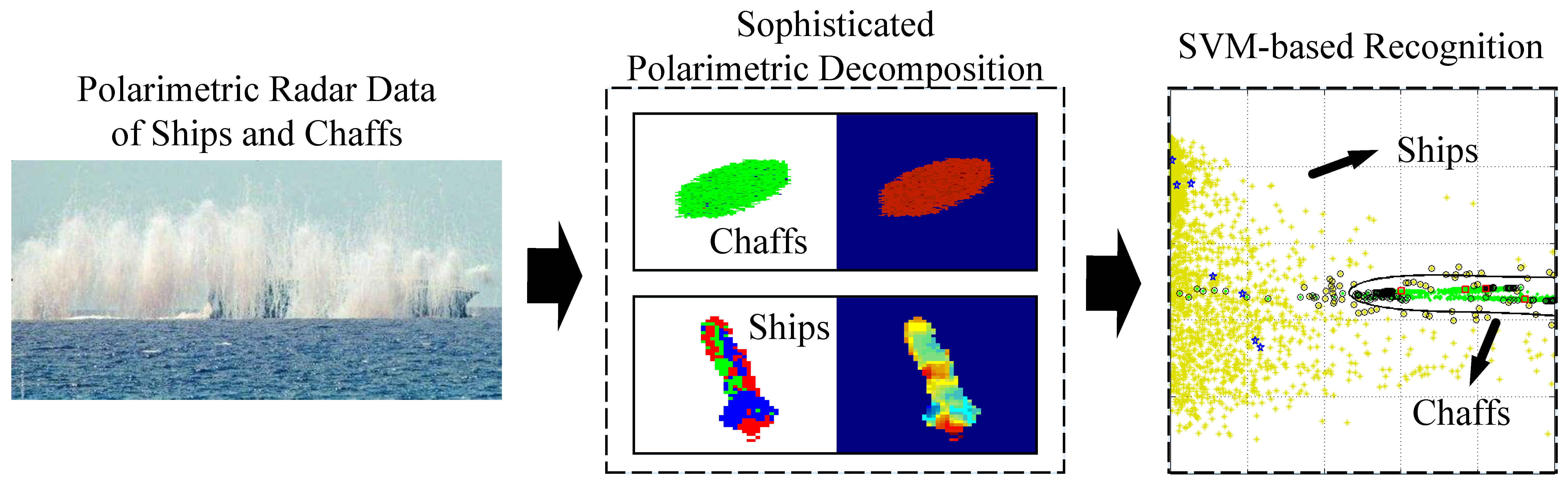
Ship Recognition from Chaff Clouds with Sophisticated Polarimetric Decomposition

Abstract

Ship recognition from chaff cloud jamming is challenging since they have similar dimensions and radar cross sections. In this paper, a polarimetric recognition technique with sophisticated polarimetric decomposition is proposed. To this end, a seven-component model-based decomposition is first put forward by integrating three sophisticated scattering models, thus the dominant and local scattering of ships can be characterized accurately. According to the derived scattering contributions, a robust discrimination feature is then designed based on the concept of contrast and suppression. Coupled with the average scattering angle estimated from eigen-based decomposition, the constructed feature vector is inputted into the support vector machine and the recognition is finally fulfilled. The proposed method is tested on simulated and real polarimetric radar data and the results demonstrate that the proposed method achieves the highest recognition rate of over 98%, which outperforms the state-of-the-art methods.

1. Introduction

Chaffs are widely applied to the passive jamming of radars due to their intense scattering induced by the resonances with electromagnetic waves. Releasing chaff clouds which have the approximate dimensions and radar cross sections (RCSs) as targets has posed serious challenges to radar recognition performance [1,2,3,4], as shown in Figure 1. Thus, the countermeasure against chaff cloud jamming, especially ship recognition from chaff cloud jamming, has significant military value.

Among current developments, integrating polarimetric techniques with radar systems has become the most concerning and pivotal direction. This is not only because many seekers and radars have polarization measurement capability, but also because the scattering mechanism can be completely described and effectively identified according to the polarimetric returns. There is numerous research conducted on the polarimetric recognition of ships from chaff clouds. Shao et al. recognized ships from chaff clouds on the basis of the ratio of co-polarized and cross-polarized components [5]. To further highlight the ratio differences, a non-linear polarization transformation is proposed by Shao et al. [6] and Li et al. [7]. Aiming at weighted chaff clouds, Li et al. performed the recognition based on their polarimetric statistical property [8]. However, it loses its effectiveness when dealing with targets whose dominant mechanism is no longer double-bounce scattering. Tang et al. investigated the recognition problem by considering the polarization-RCS ratio and the corresponding probability density function [9]. Nevertheless, the involved distribution hypothesis is overly simple and idealistic. Without any prior knowledge, Yang et al. suppressed the chaff cloud jamming by adopting the polarization oblique projection [10], yet it demanded the real-time estimation of jamming polarization parameters. Cui et al. designed the radar echo polarization ratio to identify the chaff interference, however, it turns out to be un-robust because only simulated data and single polarization information are considered [11]. By further mining the polarization ratio information, Hu et al. used the corresponding arctangent angle to distinguish chaff clouds from ships. Despite this, it is sensitive to the random orientation of chaff clouds [12].

To address the aforementioned issues, a discrimination feature on the basis of sophisticated model-based decomposition (MBD), along with a ship recognition scheme, is proposed in this paper. The MBD is considered due to its ease of implementation followed by an accurate interpretation and the physical relevance of scattering contributions to the scatterers [13,14]. The main work includes the following aspects. First, to accurately characterize the scattering of local complex structures on ships, three sophisticated scattering models are incorporated and thus a seven-component model-based decomposition is proposed. Second, to highlight the scattering differences between the ships and chaff clouds, a scattering contribution-based discrimination feature is designed according to the concept of contrast and suppression. Finally, through inputting the constructed and the average scattering angle features, a support vector machine-based classification scheme is presented, and thus the ship recognition is accomplished. Simulated and real polarimetric radar data are applied for the verification, and the results demonstrate that easy implementation and a high recognition rate make the proposed method practical and effective.

2. Methodology

2.1. Sophisticated Scattering Models

As the most typical structure of ships, the existence of dihedral will generate intense double-bounce scattering power. Nevertheless, once the relative orientation between the radar platform and dihedral shifts, the double-bounce scattering no longer dominates and significant cross-polarized responses will alternatively be induced [15,16]. Due to the improper scattering modeling, traditional MBD methods cannot identify this change and therefore they suffer deficiencies in accurate characterization of ship scattering. Given this, the proposed decomposition scheme applies the first sophisticated scattering model, i.e., the cross-scattering model (CSM) to address this issue [17,18]. The CSM is formed from a rotated dihedral structure, considering its orientation angle, which has the following form:

$${[\mathit{T}]}_{\mathrm{CRO}}=\left[\begin{array}{ccc}0& 0& 0\\ 0& (15-\cos (4{\theta }_{\mathrm{OA}})))/30& 0\\ 0& 0& (15+\cos (4{\theta }_{\mathrm{OA}})))/30\end{array}\right],{\theta }_{\mathrm{OA}}=\frac{1}{4}({\tan }^{-1}\frac{2\mathrm{Im}(T_{23})}{T_{22}-T_{33}})$$

(1)

where ${\theta }_{\mathrm{OA}}$ denotes the corresponding orientation angle. $T_{22}$, $T_{23}$, and $T_{33}$ are the elements of the coherency matrix, as also shown in Equation (4). The CSM has been proven to be effective in separating the cross-polarized components caused by oriented dihedrals from the overall cross-polarized components. As a result, it is expected that incorporating the CSM can compensate for the cross-polarized power of oriented dihedrals, which is lost in the traditional MBD methods.

On the other hand, it has been verified that the coherency matrix does not obey a reflection symmetry assumption in ship scattering scenarios [19,20]. This is intuitively reflected in that the real and imaginary parts of the $T_{13}$ term are not equal to zero. However, the traditional MBD methods generally ignore this term, which is inevitably subject to a reflection symmetry assumption and causes an apparent loss of polarimetric information. Therefore, to further utilize polarimetric information and to relieve the constraint of the reflection symmetry assumption, the $T_{13}$ term should be accounted for by certain scattering models in the MBD. To this end, two extra sophisticated scattering models, i.e., the ±45° oriented dipole (OD) and ±45° oriented quarter-wave (OQW) scattering models [21,22] are further integrated into the proposed decomposition scheme.

According to [21], the ±45° OD and ±45° OQW scattering models are derived according to the combination of oriented dipoles with specific distances. Concretely speaking, the coherency matrix of the ±45° OD and ±45° OQW scattering models can be obtained by the inner product of Pauli vectors of the corresponding scattering matrices, i.e.,

$${[\mathit{T}]}_{OD}^{\pm {45}^{°}}=\mathrm{vec}({[\mathit{S}]}_{OD}^{\pm {45}^{°}})\cdot \mathrm{vec}{({[\mathit{S}]}_{OD}^{\pm {45}^{°}})}^{\mathrm{H}}=\frac{1}{2}\left[\begin{array}{ccc}1& 0& \pm 1\\ 0& 0& 0\\ \pm 1& 0& 1\end{array}\right].$$

(2)

$${[\mathit{T}]}_{OQW}^{\pm {45}^{°}}=\mathrm{vec}({[\mathit{S}]}_{OQW}^{\pm {45}^{°}})\cdot \mathrm{vec}{({[\mathit{S}]}_{OQW}^{\pm {45}^{°}})}^{\mathrm{H}}=\frac{1}{2}\left[\begin{array}{ccc}1& 0& \mp j\\ 0& 0& 0\\ \pm j& 0& 1\end{array}\right].$$

(3)

where the notation $\mathrm{vec}(\cdot )$ and the superscript H indicate the vectorization and conjugate transpose manipulations, respectively. $[\mathit{S}]$ denotes the Sinclair matrix, which is obtained by the summation of the Sinclair matrices of the oriented dipoles located at different distances. In traditional MBDs, since the input data and scattering models cannot fit perfectly, ±45° OD and ±45° OQW scattering are regarded as residuals and are omitted directly. Meanwhile, these two scatterings exist widely and correspond to different scattering structures in reality.

Let us go deeper into the scattering analysis of ships, as presented in Figure 2. As is generally known, the most remarkable is the surface or double-bounce scattering, which occurs on the deck or ship–sea dihedrals (or ship dihedrals). Additionally, there exist certain parts of helix scattering and cross scattering, as introduced before. A more noticeable observation is that the complex superstructures composed of dipole-like structures (such as towers, antennas, and guardrails) on ships can induce distinct ±45° OD and ±45° OQW scattering. This explains that integrating the ±45° OD and ±45° OQW scattering models into the decomposition scheme can achieve the refined characterization of ship scattering. It should be noted that in the volume scattering models, the multiple scattering happens on different structures on ships, barring the helix, cross, ±45°OD, and ±45° OQW scatterers, which are accounted for in the complex structure scattering components.

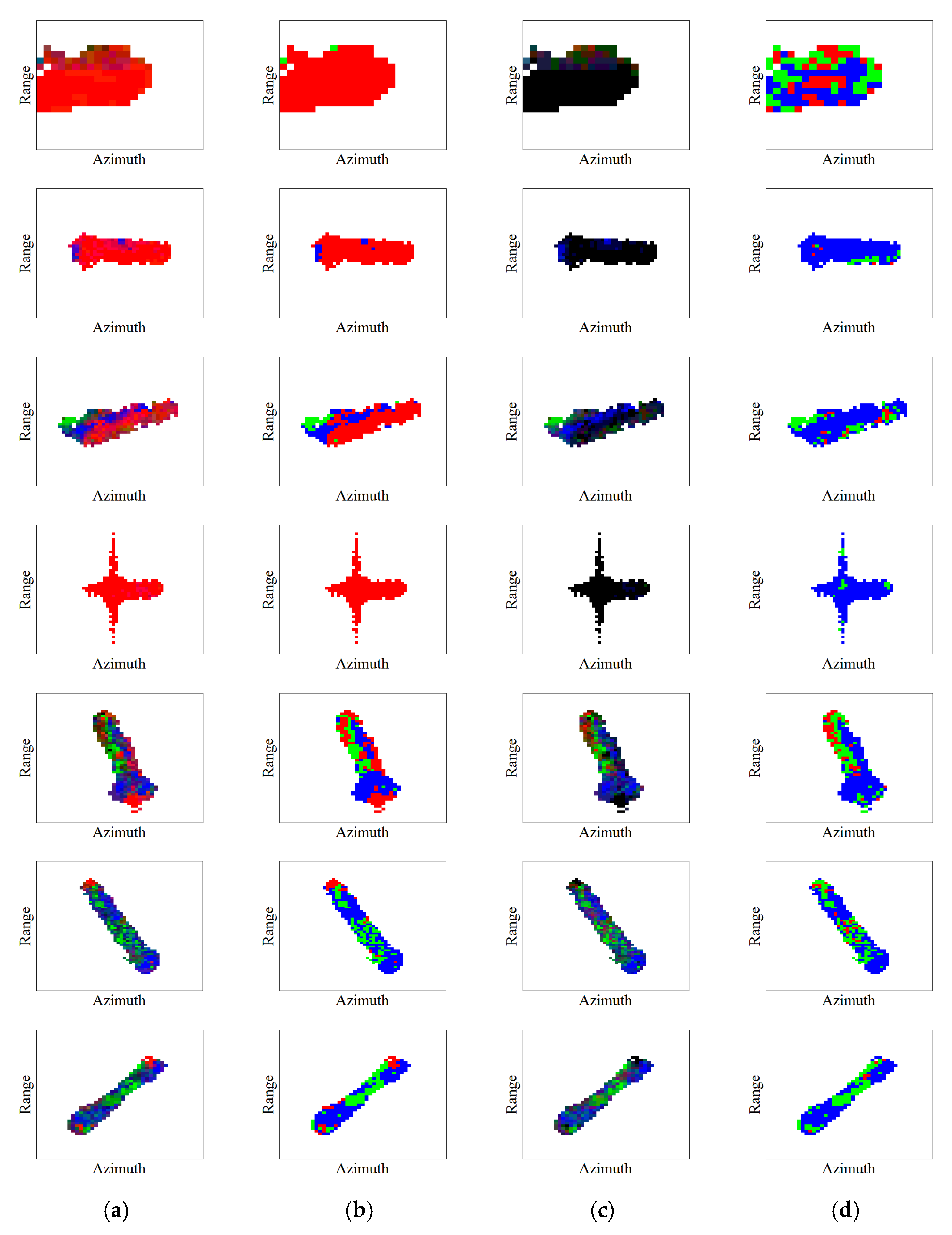
2.2. Seven-Component Model-Based Decomposition

In the monostatic backscattering case, the reciprocity constrains the Sinclair matrix to be symmetrical, thus the corresponding coherency matrix can be presented as

$$\langle [\mathit{T}]\rangle =\langle {\mathit{k}}_{3\mathrm{p}}{\mathit{k}}_{3\mathrm{p}}^{\mathrm{H}}\rangle =\left[\begin{array}{ccc}{T}_{11}& T_{12}& T_{13}\\ T_{21}& T_{22}& T_{23}\\ T_{31}& T_{32}& T_{33}\end{array}\right]$$

(4)

where ${\mathit{k}}_{3\mathrm{p}}$ represents the Pauli vector and the notation $\langle \rangle$ indicates the ensemble averaging. According to the above sophisticated scattering models, the proposed seven-component decomposition is presented as the weighted sum of several canonical scattering, i.e.,

$$\langle [\mathit{T}]\rangle =f_{\mathrm{S}}{[\mathit{T}]}_{\mathrm{S}}+f_{\mathrm{D}}{[\mathit{T}]}_{\mathrm{D}}+f_{\mathrm{H}}{[\mathit{T}]}_{\mathrm{H}}+f_{\mathrm{V}}{[\mathit{T}]}_{\mathrm{V}}+f_{\mathrm{CRO}}{[\mathit{T}]}_{\mathrm{CRO}}+f_{\mathrm{OD}}{[\mathit{T}]}_{\mathrm{OD}}+f_{\mathrm{OQW}}{[\mathit{T}]}_{\mathrm{OQW}}$$

where ${[\mathit{T}]}_{\mathrm{S}}$, ${[\mathit{T}]}_{\mathrm{D}}$, ${[\mathit{T}]}_{\mathrm{H}}$, and ${[\mathit{T}]}_{\mathrm{V}}$ are, respectively, the models of surface, double-bounce, helix, and volume scattering in the Yamaguchi four-component decomposition [14] with the following mathematical forms

$$\begin{array}{l}{[\mathit{T}]}_{\mathrm{S}}=\left[\begin{array}{ccc}1& {\mathsf{\beta }}^{\ast }& 0\\ \mathsf{\beta }& |\mathsf{\beta }{|}^2& 0\\ 0& 0& 0\end{array}\right],{[\mathit{T}]}_{\mathrm{D}}=\left[\begin{array}{ccc}|\mathsf{\alpha }{|}^2& \mathsf{\alpha }& 0\\ {\mathsf{\alpha }}^{\ast }& 1& 0\\ 0& 0& 0\end{array}\right]\\ {[\mathit{T}]}_{\mathrm{H}}=\frac{1}{2}\left[\begin{array}{ccc}0& 0& 0\\ 0& 1& \pm j\\ 0& \mp j& 1\end{array}\right],{[\mathit{T}]}_{\mathrm{V}}=\frac{1}{4}\left[\begin{array}{ccc}2& 0& 0\\ 0& 1& 0\\ 0& 0& 1\end{array}\right].\end{array}$$

(5)

wherein $\mathsf{\alpha }$ and $\mathsf{\beta }$ denote the model parameters of double-bounce scattering and surface scattering, respectively. $f_{\mathrm{S}}$, $f_{\mathrm{D}}$, $f_{\mathrm{H}}$, $f_{\mathrm{V}}$, $f_{\mathrm{CRO}}$, $f_{\mathrm{OD}}$, and $f_{\mathrm{OQW}}$ are the corresponding scattering coefficients to be estimated. According to the aforementioned scattering models, one set of equations can be achieved, i.e.,

$$\begin{array}{l}{f}_{\mathrm{S}}+f_{\mathrm{D}}|\alpha {|}^2+\frac{f_{\mathrm{V}}}{2}+\frac{f_{\mathrm{OD}}}{2}+\frac{f_{\mathrm{OQW}}}{2}=T_{11}\\ f_{\mathrm{S}}|\beta {|}^2+f_{\mathrm{D}}+\frac{f_{\mathrm{V}}}{4}+\frac{f_{\mathrm{H}}}{2}+f_{\mathrm{CRO}}\frac{15-\cos (4{\theta }_{\mathrm{OA}})}{30}=T_{22}\\ \frac{f_{\mathrm{V}}}{4}+\frac{f_{\mathrm{H}}}{2}+f_{\mathrm{CRO}}\frac{15+\cos (4{\theta }_{\mathrm{OA}})}{30}+\frac{f_{\mathrm{OD}}}{2}+\frac{f_{\mathrm{OQW}}}{2}=T_{33}\\ f_{\mathrm{S}}{\beta }^{\ast }+f_{\mathrm{D}}\alpha =T_{12}\\ \frac{f_{\mathrm{H}}}{2}=|\mathrm{Im}(T_{23})|\\ \frac{f_{\mathrm{OD}}}{2}=\mathrm{Re}(T_{13})\\ \frac{f_{\mathrm{OQW}}}{2}=|\mathrm{Im}(T_{13})|.\end{array}$$

(6)

Apparently, there are nine unknowns and eight observations in Equation (6). To address the underdetermined problem, certain assumptions need to be made in order to reduce the unknowns. According to the sign of $T_{11}-T_{22}+f_{\mathrm{H}}/2-f_{\mathrm{OD}}/2-f_{\mathrm{OQW}}/2$, one of the unknowns can be predetermined [23,24]. If $T_{11}-T_{22}+f_{\mathrm{H}}/2-f_{\mathrm{OD}}/2-f_{\mathrm{OQW}}/2>0$, then the dominant mechanism of the remaining matrix is identified as surface scattering, which leads to $f_{\mathrm{D}}=0$. Otherwise, the double-bounce scattering dominates in the remaining matrix, thus $f_{\mathrm{S}}=0$. Although the resulting equations are compact, the analytic solutions are still complicated. Considering this, the second and third equations in Equation (6) are rearranged and simplified as follows to clarify the results:

$$\begin{array}{l}{T}_{11}-T_{22}+\frac{f_{\mathrm{H}}}{2}-\frac{f_{\mathrm{OD}}}{2}-\frac{f_{\mathrm{OQW}}}{2}>0:f_{\mathrm{S}}|\beta {|}^2-f_{\mathrm{CRO}}\frac{\cos (4{\theta }_{\mathrm{OA}})}{15}-\frac{f_{\mathrm{OD}}}{2}-\frac{f_{\mathrm{OQW}}}{2}=T_{22}-T_{33}\\ T_{11}-T_{22}+\frac{f_{\mathrm{H}}}{2}-\frac{f_{\mathrm{OD}}}{2}-\frac{f_{\mathrm{OQW}}}{2}<0:f_{\mathrm{D}}-f_{\mathrm{CRO}}\frac{\cos (4{\theta }_{\mathrm{OA}})}{15}-\frac{f_{\mathrm{OD}}}{2}-\frac{f_{\mathrm{OQW}}}{2}=T_{22}-T_{33}.\end{array}$$

(7)

Further, the $f_{\mathrm{CRO}}\cos (4{\theta }_{\mathrm{OA}})/15$ can be ignored because both $f_{\mathrm{CRO}}$ and $\cos (4{\theta }_{\mathrm{OA}})/15$ are small compared to the other terms. In this case, $f_{\mathrm{S}}$ and $f_{\mathrm{D}}$ can be directly obtained according to the $T_{12}$ term. Once the surface or double-bounce scattering coefficient is determined, the rest of the scattering coefficients can be calculated and their expressions are presented as

$$\begin{array}{l}{T}_{11}-T_{22}+\frac{f_{\mathrm{H}}}{2}-\frac{f_{\mathrm{OD}}}{2}-\frac{f_{\mathrm{OQW}}}{2}>0:f_{\mathrm{D}}=0,f_{\mathrm{H}}=2\left|\mathrm{Im}(T_{23})\right|,f_{\mathrm{OD}}=2\left|\mathrm{Re}(T_{13})\right|,f_{\mathrm{OQW}}=2\left|\mathrm{Im}(T_{13})\right|\\ f_{\mathrm{S}}=\frac{{\left|T_{12}\right|}^2}{T_{11}-T_{22}+\frac{f_{\mathrm{OD}}}{2}+\frac{f_{\mathrm{OQW}}}{2}},f_{\mathrm{V}}=2(T_{11}-f_{\mathrm{S}}-\frac{f_{\mathrm{OD}}}{2}-\frac{f_{\mathrm{OQW}}}{2}),f_{\mathrm{CRO}}=\frac{4T_{33}-2f_{\mathrm{H}}-f_{\mathrm{V}}-2f_{\mathrm{OD}}-2f_{\mathrm{OQW}}}{\frac{30+2\cos (4{\theta }_{\mathrm{OA}})}{15}}.\end{array}$$

(8)

or

$$\begin{array}{l}{T}_{11}-T_{22}+\frac{f_{\mathrm{H}}}{2}-\frac{f_{\mathrm{OD}}}{2}-\frac{f_{\mathrm{OQW}}}{2}<0:f_{\mathrm{S}}=0,f_{\mathrm{H}}=2\left|\mathrm{Im}(T_{23})\right|,f_{\mathrm{OD}}=2\left|\mathrm{Re}(T_{13})\right|,f_{\mathrm{OQW}}=2\left|\mathrm{Im}(T_{13})\right|\\ f_{\mathrm{D}}=T_{11}-T_{22}+\frac{f_{\mathrm{OD}}}{2}+\frac{f_{\mathrm{OQW}}}{2},f_{\mathrm{V}}=2(T_{11}-\frac{f_{\mathrm{OD}}}{2}-\frac{f_{\mathrm{OQW}}}{2}-\frac{{\left|T_{12}\right|}^2}{f_{\mathrm{D}}}),f_{\mathrm{CRO}}=\frac{4T_{33}-2f_{\mathrm{H}}-f_{\mathrm{V}}-2f_{\mathrm{OD}}-2f_{\mathrm{OQW}}}{\frac{30+2\cos (4{\theta }_{\mathrm{OA}})}{15}}.\end{array}$$

(9)

As a result, the surface, double-bounce, volume, helix, cross, ±45° OD, and ±45° OQW scattering contributions are respectively estimated as

$$P_{\mathrm{S}}=f_{\mathrm{S}}(1+|\beta {|}^2),P_{\mathrm{D}}=f_{\mathrm{D}}(1+|\alpha {|}^2),P_{\mathrm{V}}=f_{\mathrm{V}},P_{\mathrm{H}}=f_{\mathrm{H}},P_{\mathrm{CRO}}=f_{\mathrm{CRO}},P_{\mathrm{OD}}=f_{\mathrm{OD}},P_{\mathrm{OQW}}=f_{\mathrm{OQW}}.$$

(10)

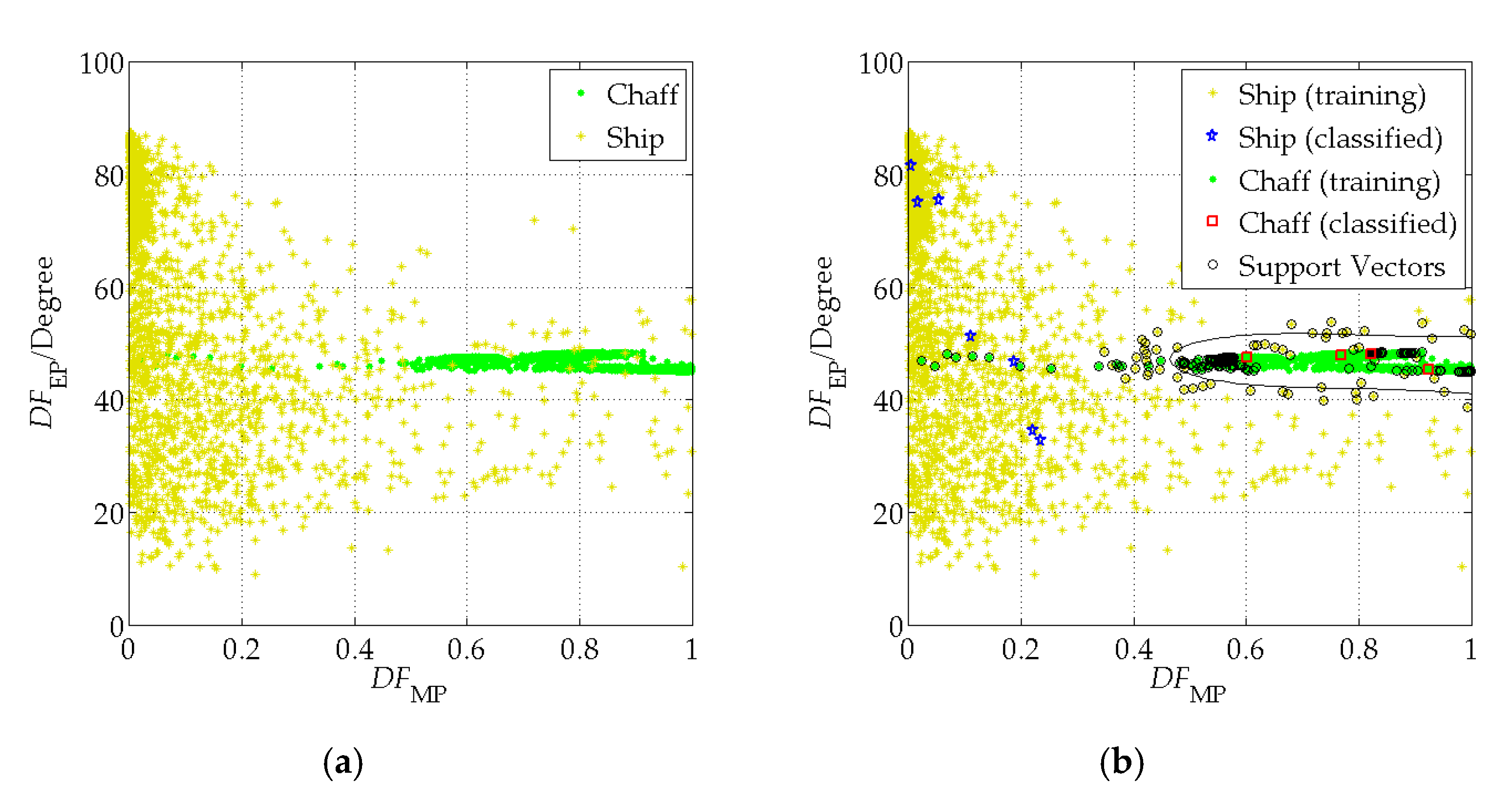
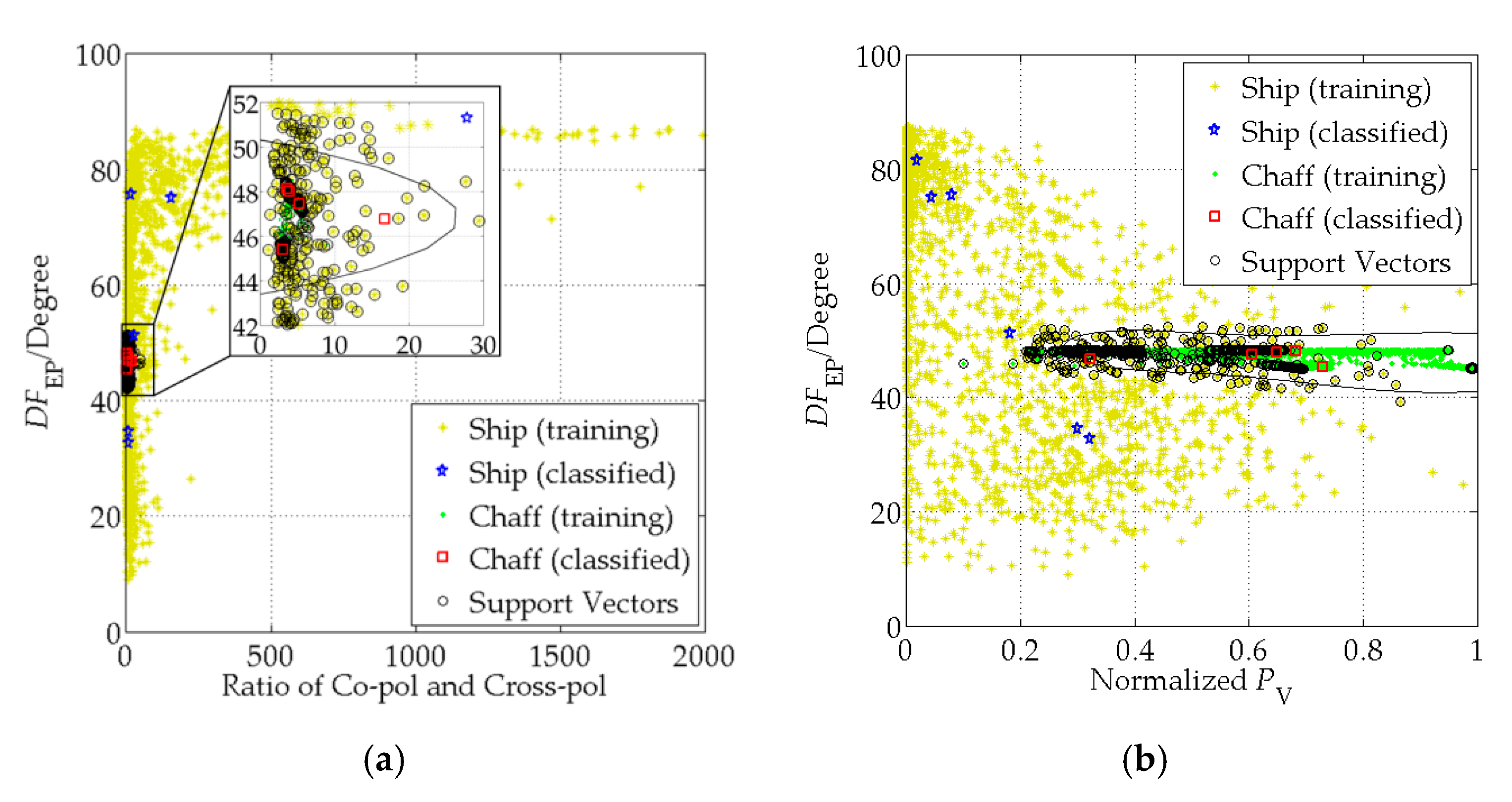
2.3. Discrimination Feature Construction

In order to achieve the optimal jamming, the length of a single chaff is generally half the wavelength of radar, which makes it equivalent to a dipole. As a result, the essential scattering mechanism of chaff clouds is volume scattering. Meanwhile, for ships, the dominant scattering mechanisms interpreted by the seven-component decomposition are surface scattering or double-bounce scattering. This is well-founded, since ships are mainly composed of flat planes (decks) and dihedral structures (broadside–sea configurations and deck-hatches). Therefore, the volume scattering contribution can be treated as a candidate feature for discrimination.

On the other hand, as chaff clouds are essentially dipoles and their orientations are randomly distributed, the reflection symmetry is generally present. This results in the complex structure scattering (the sum of helix, cross, ±45° OD, and ±45° OQW scattering) in the seven-component decomposition being negligible for chaff clouds. In contrast, due to the existence of complex superstructures, ships generally exhibit considerable complex structure scattering. Accordingly, to highlight the scattering difference, the model-based discrimination feature is proposed as

$$D{F}_{\mathrm{MP}}=\frac{\left|P_{\mathrm{V}}-P_{\mathrm{COMP}}\right|}{\mathrm{SPAN}}=\frac{\left|P_{\mathrm{V}}-P_{\mathrm{H}}-P_{\mathrm{CRO}}-P_{\mathrm{OD}}-P_{\mathrm{OQW}}\right|}{\mathrm{SPAN}}(0\le D{F}_{\mathrm{MP}}\le 1).$$

(11)

where $\mathrm{SPAN}$ denotes the total scattering power, which limits the value of $D{F}_{\mathrm{MP}}$ ranges from 0 to 1. As noted, the incorporation of $P_{\mathrm{COMP}}$ barely has an effect on the change of $D{F}_{\mathrm{MP}}$ for chaff clouds, making it stay at a relatively high level. Whereas, for ships, the subtraction can remarkably reduce the value of $D{F}_{\mathrm{MP}}$, thus the discrimination can be easily realized.

Out of consideration for completeness, the feature derived from eigen-based polarimetric decomposition is considered as well. The eigen-based decomposition, known as Cloude decomposition, employs a three-level Bernoulli model to generate estimates of the average target scattering matrix parameters, based on an eigenvalue analysis of the coherency matrix [25]. In Cloude decomposition, the value of average scattering angle $\overline{\alpha }$ is related with the physics behind the scattering process. With its value increasing from 0° to 45° and then to 90°, the underlying scattering corresponds to a continuous change from surface scattering to dipole scattering, and eventually to double-bounce scattering [26,27,28]. Considering this, the eigen-based discrimination feature is put forward as

$$D{F}_{\mathrm{EP}}=\overline{\alpha }=\frac{{\lambda }_1\arccos \left|u_1^1\right|+{\lambda }_2\arccos \left|u_2^1\right|+{\lambda }_3\arccos \left|u_3^1\right|}{\mathrm{SPAN}}(0^{\circ }\le D{F}_{\mathrm{EP}}\le {90}^{\circ })$$

(12)

where ${\lambda }_i$ and $u_i$ denote the eigenvalue and eigenvector of the coherency matrix, respectively. $u_i^1$ represents the first element of the i-th eigenvector. As analyzed, $D{F}_{\mathrm{EP}}$ will lead to a narrow range around 45° for chaff clouds due to the dominated dipole scattering. With regard to ships, their corresponding $D{F}_{\mathrm{EP}}$ will span from 0° to 90° indefinitely, since the dominant scattering is not persistent. Thus, this feature is expected to further enhance the discrimination performance.

2.4. SVM-Based Ship Recognition

With the construction of the abovementioned discrimination features, this subsection adopts the support vector machine (SVM) [29] to fulfill the ship recognition. The SVM is a very powerful classification method that is used to solve a two-class pattern recognition problem. The most well established SVM is a linear classifier, in which the classification is made by predicting each input’s member class. A more accurate definition would state that a hyperplane is built in the SVM in order to classify all inputs in a multidimensional space. The closest points to the classification margin are known as support vectors. The goal is to find the optimal separating hyperplane between two classes, by maximizing the margin between the support vectors.

In general, it is difficult to distinguish the two classes using a linear hyperplane. This paper utilizes a kernel function named the Gaussian radial basis function (RBF) to map the original feature sets ($D{F}_{\mathrm{MP}}$, $D{F}_{\mathrm{EP}}$) into a higher dimensional space, so that the transformed feature sets can be linearly separable. It is beneficial to accelerate the training procedure and decrease the training error. Compared with the traditional linear SVM classifier, the SVM with RBF kernel has the advantages of strong generalization ability, quick convergence speed, and fine training effect with a small set of samples. The feature set of the training samples is fed into the optimization objective function of the SVM classifier, and the optimal hyperplane can be obtained accordingly [29]. For simplicity, the details of the training procedure are ignored.

The procedure of the SVM-based recognition involves the following concise steps: (1) Collection of training data, (2) Construction of feature and feature vectors, (3) Machine learning with training data, (4) Obtaining of the SVM model, and (5) Classification with the SVM model and test data. The flowchart of the proposed SVM-based ship recognition scheme is shown in Figure 3.

3. Results

3.1. Data Decription

This work applies the simulated polarimetric radar data for chaff clouds, as in [30]. Three cases of typical distributions of chaff clouds are simulated, i.e., Case 1 with uniform distribution for the orientation angle and sinusoidal distribution for the zenith angle, Case 2 with the orientation angle obeying the uniform distribution while the zenith angle is distributed at a specific interval, and Case 3 with the orientation angle with uniform distribution and the zenith angle with normal distribution (centering at 20° and 90° for Case 3-1 and Case 3-2, respectively) [30]. In order to attain similar dimensions as ships, assuming that 20,000 chaffs are initially dispersed within a cube space with size of 30 m after 120 s, the results of the diffused chaff clouds in different cases are simulated, as given in Figure 4a–d. To save space, only the HH polarization intensity images are presented.

The real polarimetric radar data for ships is acquired from the Radarsat-2 spaceborne system over a test site in Vancouver, Canada. To acquire a visually pleasing representation, the multilook processing is, respectively, performed with factors 2 and 1 in the azimuth and range direction, which results in a resolution of 4.87 m × 4.73 m in the ground area. Figure 4e shows the C-band Pauli color-coded images (1693 pixels × 1501 pixels), where seven ships (denoted by T1–T7) are marked by red rectangles.

3.2. Decomposition Results

Using the proposed seven-component decomposition, the color composite results for chaff clouds are shown in Figure 5. As shown in Figure 5, the first row presents the results where the red, green, and blue channels denote the double-bounce, volume, and surface scattering contributions, respectively. In the second row, the results are generated according to the dominant scattering among the components. For example, the scattering point is defined as [0,1,0] if the volume scattering dominates. In addition, the normalized scattering contribution statistics are given in

Table 1. Scattering contribution statistics for chaff clouds.

Chaff Clouds	Case 1	Case 2	Case 3-1	Case 3-2
Surface scattering	2.69%	22.25%	38.91%	16.90%
Double-bounce scattering	0.88%	0.08%	0.18%	0.09%
Volume scattering	93.62%	77.25%	60.55%	82.51%
Helix scattering	0.53%	0.40%	0.36%	0.42%
Cross scattering	0.45%	0.00%	0.00%	0.01%
±45° OD scattering	0.92%	0.00%	0.00%	0.02%
±45° OQW scattering	0.90%	0.01%	0.00%	0.03%
Complex structure scattering	2.8%	0.41%	0.36%	0.48%

.

From the qualitative and quantitative results, it is obvious that almost all of the chaff clouds exhibit intense volume scattering, except several scattering points that have the surface or double-bounce scattering as dominant. On the other hand, in addition to the small amount of the complex structure scattering for Case 1 (2.8%), it barely exists in other cases (notice that the helix scattering contributes the most). The above observations demonstrate that the proposed decomposition can accurately characterize the chaff cloud scattering.

Figure 6 shows the decomposed results for ships T1 to T7 in the first to seventh rows, respectively. As shown in Figure 6, the first and third columns present the color composite results where the red, green, and blue channels denote the double-bounce/complex structure, volume, and surface scattering contributions, respectively. Meanwhile, the corresponding RGB results generated from the interpreted dominant scattering are given in the second and fourth columns. Similarly, the normalized scattering contribution statistics for ships are given in

Table 2. Scattering contribution statistics for ships.

Ships	T1	T2	T3	T4	T5	T6	T7
Surface scattering	4.79%	12.20%	30.78%	3.65%	30.09%	41.78%	40.69%
Double-bounce scattering	83.80%	85.71%	55.30%	95.49%	32.59%	12.50%	12.22%
Volume scattering	5.46%	1.55%	7.93%	0.63%	23.95%	30.30%	33.12%
Helix scattering	2.69%	0.12%	2.41%	0.06%	7.41%	6.46%	9.99%
Cross scattering	0.19%	0.03%	0.07%	0.009%	1.36%	0.26%	0.01%
±45° OD scattering	1.49%	0.03%	1.04%	0.004%	2.67%	4.37%	2.02%
±45° OQW scattering	1.19%	0.03%	2.03%	0.008%	2.80%	4.11%	1.71%
Complex structure scattering	5.56%	0.20%	5.55%	0.09%	14.24%	15.20%	13.73%

.

As can be seen, the double-bounce scattering dominates for T1 to T5, whereas T6 and T7 have the surface scattering as dominant. These conform to reality, because ships are mainly composed of surface or double-bounce scatterers, as introduced earlier. To be specific, for T1, T2, and T4, the dihedral structures do not have orientation shifts with respect to the radar illumination. In this case, they are considered to be symmetric targets and thus intense double-bounce scattering powers are produced (83.80%, 85.71%, and 95.49%, respectively). Due to the presentation of reflection symmetry, the complex structure scattering is very weak, and therefore they exhibit black tones in the third column. With regard to other ships, their hulls are no longer parallel to the azimuth direction, and the reflection symmetry is often broken because significant cross-polarization power is induced. As a result, the complex structure scattering is noticeably present and distributed sporadically at the different locations of the ships (the red points in the fourth column), explaining that it corresponds to the scattering of specific ship superstructures. In addition, it is noticed that the volume scattering for T5, T6, and T7 is significant (23.95%, 30.30%, and 33.12%, respectively). This is mainly attributed to the multiple scattering interactions between structures.

From the above decomposition results, it can be concluded that the values of $D{F}_{\mathrm{MP}}$ for chaff clouds are larger than 0.6, whereas the values of $D{F}_{\mathrm{MP}}$ for ships are generally lower than 0.15. Therefore, it is expected that the proposed $D{F}_{\mathrm{MP}}$ feature can be well applied to the recognition.

3.3. Ship Recognition Performance

To make full use of the information derived from polarimetric decomposition, the average scattering angle, i.e., $D{F}_{\mathrm{EP}}$, is incorporated to enhance the recognition performance. Figure 7 and Figure 8 give the histograms of $D{F}_{\mathrm{EP}}$ for chaff clouds and ships, respectively. It can be seen that for chaff clouds in different cases, almost all of $D{F}_{\mathrm{EP}}$ have values of about 45°, which is consistent with the theoretical analysis. Meanwhile, for ships, in addition to T1, T2, and T4 (their $D{F}_{\mathrm{EP}}$ values lie between 50° and 90°), the calculated $D{F}_{\mathrm{EP}}$ does not correspond to double-bounce scattering. This actually relates to the complex structures of ships, which validates the effectiveness of the complex structure scattering from another side.

In order to visualize the difference, the scatter diagram of data points in the two dimensional $D{F}_{\mathrm{MP}}$ − $D{F}_{\mathrm{EP}}$ plane is shown in Figure 9a. It is intuitive that a special pattern of green colors is clearly noticed, indicating that ships and chaff clouds can be easily distinguished in the proposed plane. With the constructed discrimination features, the recognition of ships and chaff clouds is implemented through obtaining the trained SVM model. All the data points of ships and chaff clouds are used for training, while the corresponding averages, i.e., seven data points of ships and four data points of chaff clouds, are selected to be classified (i.e., for testing).

Figure 9b presents the SVM-based recognition results, where the hollow circles represent the support vectors. As expected, the recognition curve can be easily and clearly drawn due to the favorable discrimination abilities of the constructed features. Moreover, it is observed that both ships (the blue stars) and chaff clouds (the red rectangles) are correctly classified. For quantitative evaluation, the correct and missed recognition points of ships and chaff clouds are counted. Among 1838 ship points, only 22 points are wrongly recognized as chaff clouds. Meanwhile, there are a total of 5495 chaff cloud points and only 13 of them are categorized as ships. In other words, the recognition rate for ships reaches 98.80%, indicating that the proposed method can accurately and effectively recognize ships from chaff cloud jamming.

4. Discussion

In order to demonstrate the superiority of the proposed discrimination feature, this subsection designs several composite methods according to control variate techniques for discussion and comparison. Since the cross-polarized component is significant larger than the co-polarized component for chaff clouds, while the situation for ships is quite the reverse, the ratio of co- and cross-polarized components (RCP) is a favorable feature for discrimination [5]. Therefore, the first composite method is the combination of the RCP, $D{F}_{\mathrm{EP}}$, and SVM (denoted as RCP + $D{F}_{\mathrm{EP}}$ + SVM). On the other hand, to investigate its contribution, the complex structure scattering is removed from $D{F}_{\mathrm{MP}}$ and only the volume scattering is retained. Moreover, the volume scattering contribution estimated from the general four-component decomposition (G4D) [31] is utilized, as it can effectively reduce the volume scattering for man-made structures. Accordingly, the second composite method is designed to contain three aspects: the volume scattering, $D{F}_{\mathrm{EP}}$, and SVM (denoted as GPv + $D{F}_{\mathrm{EP}}$ + SVM).

Figure 10 presents the corresponding recognition results. With regard to the RCP + $D{F}_{\mathrm{EP}}$ + SVM method, it can be observed that the RCPs for ships cover a wide range, whereas those for chaff clouds are only distributed in a narrow interval. Despite this, a considerable number of ships are divided into the chaff cloud category according to the recognition curve, leading to distinct missed recognition. Regarding the GPv + $D{F}_{\mathrm{EP}}$ + SVM method, the recognition performance is slightly better because the recognition curve excludes more chaff cloud points, yet there is still obvious mixing. What is noteworthy is that the misclassification occurs in both methods, which is reflected in five testing points that are classified as chaff clouds (the red rectangles), while there are only four chaff cloud testing points.

To quantify the results, four indices, i.e., correct recognition (CR), missed recognition (MR), false recognition (FR), and classification accuracy (CA) are applied, and the corresponding values are shown in

Table 3. Quantitative recognition performance for different composite methods.

Composite Method	CR	MR	FR	CA
The Proposed	98.80%	1.20%	0.25%	100%
RCP + $D{F}_{\mathrm{EP}}$+ SVM	92.27%	7.73%	0.00%	90.90%
GPv + $D{F}_{\mathrm{EP}}$ + SVM	95.04%	4.96%	0.51%	90.90%
$D{F}_{\mathrm{MP}}$ + SVM	95.10%	4.90%	3.57%	100%
$D{F}_{\mathrm{EP}}$ + SVM	94.61%	5.39%	3.79%	90.90%

. It is intuitive that the proposed method outperforms these two methods in the CR, MR, and CA indices. As for FR, its influence can be ignored because its value stays at a very low level for all of the methods. According to the above results, it can be concluded that the proposed feature $D{F}_{\mathrm{MP}}$ has a definite advantage in the recognition compared to the RCP and the GPv. Moreover, it is important to incorporate the complex structure scattering into the feature construction, since it leads to an increment of 3% for the recognition rate.

Finally, concerning the proposed method that consists of two discrimination features and to fully explore their influences, two extra composite methods, i.e., $D{F}_{\mathrm{MP}}$ with the SVM ($D{F}_{\mathrm{MP}}$ + SVM) and $D{F}_{\mathrm{EP}}$ with the SVM ($D{F}_{\mathrm{EP}}$ + SVM), are compared. The corresponding recognition results are also listed in Table 3. By checking the index values, the $D{F}_{\mathrm{MP}}$ + SVM method is apparently superior to the $D{F}_{\mathrm{EP}}$ + SVM method. Although the differences among the first three indices are tiny, the CA index indicates that the $D{F}_{\mathrm{EP}}$ + SVM method cannot guarantee the essential correct classification. As a result, the proposed $D{F}_{\mathrm{EP}}$ feature contributes more to the performance improvement while $D{F}_{\mathrm{EP}}$ only works as an auxiliary mean.

Although the proposed method is easy to operate and certainly has superiority over the existing methods, the challenges of its implementation in the real-time radar system should be noticed. On the one hand, with the continuous improvement of resolution, the scattering models may lose their effectiveness, since the coherent and incoherent scattering exist simultaneously in a resolution cell. In this case, more refined scattering models should be introduced to accurately characterize the ship scattering. On the other hand, the presented value of nearly 99% refers more to a precision estimation than to a real accuracy that includes the trueness as important feature. As certain interrelations between simulation and detection cannot be excluded, the optimal solution would be the provision of a completely independent reference data set for the control, being aware of this massive undertaking.

5. Conclusions

Chaff clouds are one of the major hindrances to ship recognition in military applications due to their similar dimensions and radar cross sections. Considering this, this paper proposes a polarimetric recognition method from the perspective of sophisticated model-based decomposition. On the one hand, the cross, ±45° OD, and ±45° OQW scattering models are adopted and a sophisticated seven-component model-based decomposition is presented, which aims to accurately characterize the ship scattering. On the other hand, following the concept of contrast and the suppression of scattering characteristics, the scattering contributions are combined to construct a discrimination feature for the SVM-based recognition. The factors responsible for the improvement of recognition performance have been sufficiently discussed. The objective and subjective results show that the proposed discrimination feature is the best choice for ship recognition, leading to the highest recognition rate of 98.8%. Notice that the simulated chaff cloud data are applied in this study. Whereas, in reality, the measured polarimetric data acquired from the outfield experiment can be used for the offline training so as to further enhance the abilities of recognition and the real-time processing of radar systems.

References

1. Chen, J. Principles of Radar Chaff Jamming; National Defense Industry Press: Beijing, China, 2007; pp. 46–108. ISBN 9787118048780. [Google Scholar]
2. Marcus, S.W. Dynamics and radar cross section density of chaff clouds. IEEE Trans. Aerosp. Electron. Syst. 2004, 40, 93–102. [Google Scholar] [CrossRef]
3. Bendayan, M.; Garcia, A. Signal modeling of chaff in naval environment simulation. IEEE Trans. Aerosp. Electron. Syst. 2015, 51, 3161–3166. [Google Scholar] [CrossRef]
4. Seo, D.W.; Lee, J.H.; Lee, H.S. Estimation of incoherent scattered field by multiple scatterers in random media. ETRI J. 2016, 38, 141–148. [Google Scholar] [CrossRef]
5. Shao, X.H.; Xue, J.H.; Du, H. Theoretical analysis of polarization recognition between chaff cloud and ship. In Proceedings of the 2007 International Workshop on Anti-Counterfeiting, Security and Identification (ASID), Xiamen, China, 16–18 April 2007; pp. 125–129. [Google Scholar] [CrossRef]
6. Shao, X.H.; Du, H.; Xue, J.H. A target recognition method based on non-Linear polarization transformation. In Proceedings of the 2007 International Workshop on Anti-Counterfeiting, Security and Identification (ASID), Xiamen, China, 16–18 April 2007; pp. 157–163. [Google Scholar] [CrossRef]
7. Li, X.; Lin, L.S.; Shao, X.H. A target polarization recognition method for radar echoes. In Proceedings of the 2010 International Conference on Microwave and Millimeter Wave Technology, Chengdu, China, 8–11 May 2010; pp. 1644–1647. [Google Scholar] [CrossRef]
8. Li, J.L.; Zeng, Y.F.; Shen, X.J.; Xie, H. Modified polarization recognition method for chaff jamming. Radar Sci. Technol. 2015, 13, 350–355. [Google Scholar] [CrossRef]
9. Tang, B.; Li, H.M.; Sheng, X.Q. Jamming recognition method based on the full polarisation scattering matrix of chaff clouds. IET Microw. Antennas Propag. 2012, 6, 1451–1460. [Google Scholar] [CrossRef]
10. Yang, Y.; Feng, D.-J.; Wang, X.-S.; Xiao, S.-P. Polarisation oblique projection for radar seeker tracking in chaff centroid jamming environment without prior knowledge. IET Radar Sonar Navig. 2014, 8, 1195–1202. [Google Scholar] [CrossRef]
11. Cui, G.; Liu, J.; Shi, L.; Ma, J. Identification of chaff interference based on polarization parameter measurement. In Proceedings of the IEEE 13th International Conference on Electronic Measurement & Instruments, Yangzhou, China, 20–22 October 2017; pp. 1–5. [Google Scholar] [CrossRef]
12. Hu, S.; Wu, L.; Zhang, J.; Xu, J. Research on Chaff Jamming Recognition Technology of Anti-ship Missile Based on Radar Target Characteristics. In Proceedings of the IEEE 12th International Conference on Intelligent Computation Technology and Automation, Xiangtan, China, 26–27 October 2019; pp. 222–226. [Google Scholar] [CrossRef]
13. Freeman, A.; Durden, S.L. A three-component scattering model for polarimetric SAR data. IEEE Trans. Geosci. Remote Sens. 1998, 36, 963–973. [Google Scholar] [CrossRef] [Green Version]
14. Yamaguchi, Y.; Moriyama, T.; Ishido, M.; Yamada, H. Four-component scattering model for polarimetric SAR image decomposition. IEEE Trans. Geosci. Remote Sens. 2005, 43, 1699–1706. [Google Scholar] [CrossRef]
15. Quan, S.; Xiang, D.; Xiong, B.; Hu, C.; Kuang, G. A Hierarchical Extension of General Four-Component Scattering Power Decomposition. Remote Sens. 2017, 9, 1–23. [Google Scholar] [CrossRef] [Green Version]
16. Quan, S.; Xiang, D.; Xiong, B.; Kuang, G. Derivation of the Orientation Parameters in Built-up Areas: With Application to Model-based Decomposition. IEEE Trans. Geosci. Remote Sens. 2018, 56, 4714–4730. [Google Scholar] [CrossRef]
17. Xiang, D.; Ban, Y.; Su, Y. Model-based decomposition with cross scattering for polarimetric SAR urban areas. IEEE Geosci. Remote Sens. Lett. 2015, 12, 2496–2500. [Google Scholar] [CrossRef]
18. Quan, S.; Xiong, B.; Xiang, D.; Hu, C.; Kuang, G. Scattering characterization of obliquely oriented buildings from PolSAR data using eigenvalue-related model. Remote Sens. 2019, 5, 1–12. [Google Scholar] [CrossRef] [Green Version]
19. Xi, Y.; Lang, H.; Tao, Y.; Huang, L.; Pei, Z. Four-Component Model-Based Decomposition for Ship Targets using PolSAR Data. Remote Sens. 2017, 6, 1–19. [Google Scholar] [CrossRef] [Green Version]
20. Sugimoto, M.; Ouchi, K.; Nakamura, Y. On the novel use of model-based decomposition in SAR polarimetry for target detection on the sea. Remote Sens. Lett. 2013, 4, 843–852. [Google Scholar] [CrossRef]
21. Singh, G.; Yamaguchi, Y. Model-based six-component scattering matrix power decomposition. IEEE Trans. Geosci. Remote Sens. 2018, 56, 5687–5704. [Google Scholar] [CrossRef]
22. Fan, H.; Quan, S.; Dai, D.; Wang, X.; Xiao, S. Seven-Component Model-Based Decomposition for PolSAR Data with Sophisticated Scattering Models. Remote Sens. 2019, 23, 1–19. [Google Scholar] [CrossRef] [Green Version]
23. Yajima, Y.; Yamaguchi, Y.; Sato, R.; Yamada, H.; Boerner, W.M. POLSAR image analysis of wetlands using a modified four-component scattering power decomposition. IEEE Trans. Geosci. Remote Sens. 2008, 46, 1667–1673. [Google Scholar] [CrossRef]
24. Sato, A.; Yamaguchi, Y.; Singh, G.; Park, S.E. Four-component scattering power decomposition with extended volume scattering model. IEEE Geosci. Remote Sens. Lett. 2011, 9, 166–170. [Google Scholar] [CrossRef]
25. Cloude, S.R. Polarisation: Applications in Remote Sensing; Oxford University Press: New York, NY, USA, 2010; pp. 57–65. ISBN 9780191574382. [Google Scholar]
26. Lee, J.S.; Pottier, E. Polarimetric Radar Imaging: From Basics to Applications; Taylor & Francis: Boca Raton, FL, USA, 2009; pp. 85–158. ISBN 9781420054972. [Google Scholar]
27. Quan, S.; Xiong, B.; Xiang, D.; Zhao, L.; Zhang, S.; Kuang, G. Eigenvalue-based urban area extraction using polarimetric SAR data. IEEE J. Sel. Top. Appl. Earth Observ. Remote Sens. 2018, 11, 458–471. [Google Scholar] [CrossRef]
28. Touzi, R. Target Scattering Decomposition in Terms of Roll-Invariant Target Parameters. IEEE Trans. Geosci. Remote Sens. 2007, 45, 73–84. [Google Scholar] [CrossRef]
29. Cristianini, N.; Shawe-Taylor, J. An Introduction to Support Vector Machines and Other Kernel-Based Learning Methods; Cambridge University Press: Cambridge, MA, USA, 2000; pp. 198–216. ISBN 0521780195. [Google Scholar]
30. Liu, Y.; Xing, S.; Li, Y.; Hou, D.; Wang, X. Jamming recognition method based on the polarisation scattering characteristics of chaff clouds. IET Radar Sonar Navig. 2017, 11, 1689–1699. [Google Scholar] [CrossRef]
31. Chen, S.W.; Wang, X.S.; Xiao, S.P.; Sato, M. General polarimetric model-based decomposition for coherency matrix. IEEE Trans. Geosci. Remote Sens. 2013, 52, 1843–1855. [Google Scholar] [CrossRef]
Figure 1. Chaff released from a ship in an actual scenario (Courtesy: Baidu).
Remotesensing 12 01813 g001
Figure 2. Various types of scattering occurring on a ship.
Remotesensing 12 01813 g002
Figure 3. The flowchart of ship recognition based on the support vector machine.
Remotesensing 12 01813 g003
Figure 4. Simulated and real polarimetric radar data of chaff clouds and ships, respectively. (ad) The HH polarization intensity images of chaff clouds for Case 1, Case 2, Case 3-1, and Case 3-2, respectively. (e) Pauli color-coded image of Radarsat-2 with marked ships.
Remotesensing 12 01813 g004
Figure 5. Decomposition results for chaff clouds in different cases. (a) Case 1. (b) Case 2. (c) Case 3-1. (d) Case 3-2. (red: double-bounce scattering, green: volume scattering, blue: surface scattering).
Remotesensing 12 01813 g005
Figure 6. Decomposition results for ships T1 to T7 in the first to seventh rows, respectively. (a,b) Color composite results generated from the double-bounce (red), volume (green), and surface scattering (blue). (c,d) Color composite results generated from the complex structure (red), volume (green), and surface scattering (blue).
Remotesensing 12 01813 g006
Figure 7. Histograms of empty D F EP for chaff clouds. (a) Case 1. (b) Case 2. (c) Case 3-1. (d) Case 3-2.
Remotesensing 12 01813 g007
Figure 8. Histograms of D F EP for ships. (ag) T1, T2, T3, T4, T5, T6, and T7, respectively.
Remotesensing 12 01813 g008
Figure 9. Recognition results of the proposed method. (a) Distribution of data points in the two dimensional D F MP plane. (b) SVM-based classification results. Support vector machine-based classification results.
Remotesensing 12 01813 g009
Figure 10. SVM-based classification results of different composite methods. (a) The RCP + D F EP + SVM method. The composite method with the combination of the RCP, D F EP , and SVM. (b) The GPv + D F EP + SVM method. The composite method with the combination of the GPv, D F EP , and SVM.
Remotesensing 12 01813 g010