Similarity Metrics Enforcement in Seasonal Agriculture Areas Classification


Abstract

1. Introduction
1.1. Remote Sensing
1.2. Brazilian Agriculture in Numbers
2. Methods
2.1. Studied Area
2.2. IBGE Census
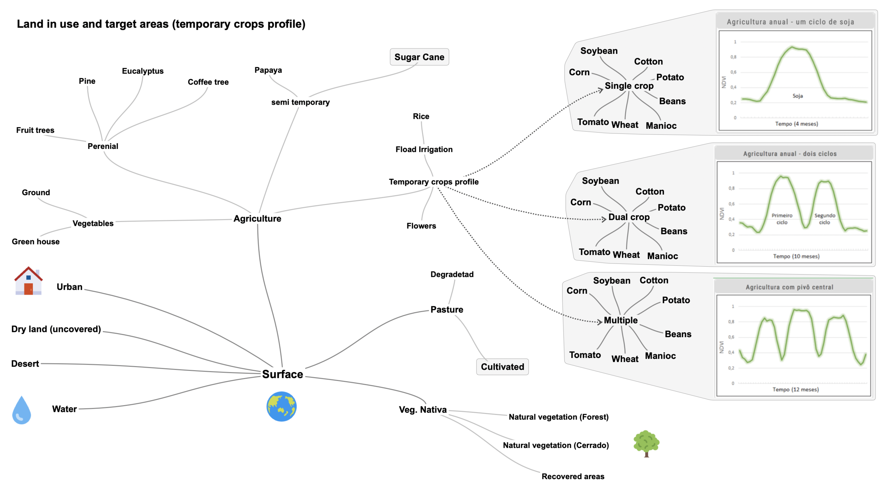
2.3. Ontology
2.4. Datasets Processing
2.5. Time-Frame
2.6. Validation
2.7. Computation Tolls
3. Results
4. Discussion
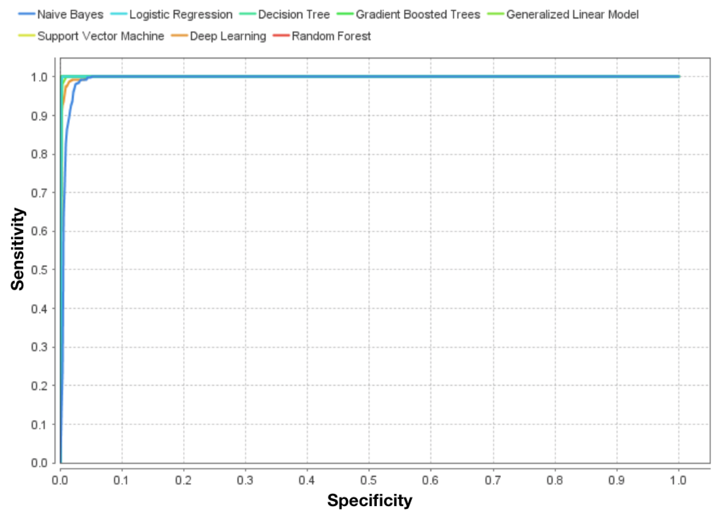
- Low: Suport Vector Machine, Deep Learning, Gradient Boosted Tree
- Moderate: Naive Bayes
- High: Logistic Regression, Decision Tree, Gradient Boosted Tree, Random Forest
5. Conclusions
- As the primary objective, the results demonstrated that the approach enhanced the classification accuracy for all tested algorithms. This is the highest accuracy for the classification of agriculture areas in Brazil, 99.6% with kappa index of 0.96 using Gradient Boosted Tree algoriothm;
- The similarity metrics worked to increase the accuracy within the context proposed, EVI data reflecting the growing season dynamics of temporary crops. The similarity metric added 3–14% points to the accuracy;
- The process increased accuracy and without extra computational cost.
- The results are robust to support policy maker and precision farming, of confidence level.
Author Contributions
Funding
Acknowledgments
Conflicts of Interest
References
- Johansson, R.; Luebehusen, E.; Morris, B.; Shannon, H.; Meyer, S. Monitoring the impacts of weather and climate extremes on global agricultural production. Weather Clim. Extrem. 2015, 10, 65–71. [Google Scholar] [CrossRef]
- Shi, Z.H.; Li, L.; Yin, W.; Ai, L.; Fang, N.F.; Song, Y.T. Use of multi-temporal Landsat images for analyzing forest transition in relation to socioeconomic factors and the environment. Int. J. Appl. Earth Obs. Geoinf. 2011, 13, 468–476. [Google Scholar] [CrossRef]
- Kaliraj, S.; Chandrasekar, N.; Magesh, N.S. Evaluation of multiple environmental factors for site-specific groundwater recharge structures in the Vaigai River upper basin, Tamil Nadu, India, using GIS-based weighted overlay analysis. Environ. Earth Sci. 2015, 74, 4355–4380. [Google Scholar] [CrossRef]
- Herman, E.; Haesen, D.; Rem, F.; Urbano, F.; Tote, C.; Bydekerke, L. Monitoring the impacts of weather and climate extremes on global agricultural production. ISPRS J. Photogramm. Remote Sens. 2015, 53, 154–162. [Google Scholar] [CrossRef]
- Lahousse, T.; Chang, K.T.; Lin, Y.H. Landslide mapping with multi-scale object-based image analysis-a case study in the Baichi watershed, Taiwan. Nat. Hazards Earth Syst. Sci. 2011, 11, 2715–2726. [Google Scholar] [CrossRef]
- Coase, R.H. The Nature of the Firm 1937. Economica 1937, 4, 386–405. [Google Scholar] [CrossRef]
- Barzel, Y.; Kochin, L.A. Ronald Coase on the Nature of Social Cost as a Key to the Problem of the Firm. Scand. J. Econ. 1992, 94, 19–31. [Google Scholar] [CrossRef]
- Guijarro, M.; Pajares, G.; Riomoros, I.; Herrera, P.J.; Burgos-Artizzu, X.P.; Ribeiro, A. Automatic segmentation of relevant textures in agricultural images. Comput. Electron. Agric. 2011, 75, 75–83. [Google Scholar] [CrossRef]
- Mulyono, S.; Pianto, T.A.; Fanany, M.; Basaruddin, T. An ensemble incremental approach of Extreme Learning Machine (ELM) For paddy growth stages classification using MODIS remote sensing images. Adv. Comput. Sci. Inf. Syst. 2013, 309–314. [Google Scholar] [CrossRef]
- Jones, H.G.; Vaughan, R.A. Remote Sensing of Vegetation: Principles, Techniques and Applications; Oxford: New York, NY, USA, 2010; p. 353. [Google Scholar] [CrossRef]
- Cariou, C.; Chehdi, K. Unsupervised nearest neighbors clustering with application to hyperspectral Images. IEEE J. Sel. Top. Signal Process. 2015, 9, 1105–1116. [Google Scholar] [CrossRef]
- Kussul, N.; Lavreniuk, M.; Skakun, S.; Shelestov, A. Deep Learning Classification of Land Cover and Crop Types Using Remote Sensing Data. IEEE Geosci. Remote Sens. Lett. 2017, 14, 778–782. [Google Scholar] [CrossRef]
- Waldner, F.; De Abelleyra, D.; Verón, S.R.; Zhang, M.; Wu, B.; Plotnikov, D.; Bartalev, S.; Lavreniuk, M.; Skakun, S.; Kussul, N.; et al. Towards a set of agrosystem-specific cropland mapping methods to address the global cropland diversity. Int. J. Remote Sens. 2016, 37. [Google Scholar] [CrossRef]
- Arvor, D.; Jonathan, M.; Meirelles, M.S.P.; Dubreuil, V.; Durieux, L. Classification of MODIS EVI time series for crop mapping in the state of Mato Grosso, Brazil. Int. J. Remote Sens. 2011, 32, 7847–7871. [Google Scholar] [CrossRef]
- Hatami, N.; Gavet, Y.; Debayle, J. Classification of Time-Series Images Using Deep Convolutional Neural Networks. In Proceedings of the 10th International Conference Machine Vision, Vienna, Austria, 13–15 November 2017; pp. 1–9. [Google Scholar] [CrossRef]
- Rezaee, M.; Mahdianpari, M.; Zhang, Y.; Salehi, B. Deep Convolutional Neural Network for Complex Wetland Classification Using Optical Remote Sensing Imagery. IEEE J. Sel. Top. Appl. Earth Obs. Remote Sens. 2018. [Google Scholar] [CrossRef]
- Transon, J.; D’Andrimont, R.; Maugnard, A.; Defourny, P. Survey of hyperspectral Earth Observation applications from space in the Sentinel-2 context. Remote Sens. 2018, 10, 157. [Google Scholar] [CrossRef]
- Chen, B.; Huang, B.; Xu, B. Multi-source remotely sensed data fusion for improving land cover classification. ISPRS J. Photogramm. Remote Sens. 2017, 124, 27–39. [Google Scholar] [CrossRef]
- Huang, B.; Wei, D.K.; Li, H.X.; Zhuang, Y.L. Using a rough set model to extract rules in dominance-based interval-valued intuitionistic fuzzy information systems. Inf. Sci. 2013, 221, 215–229. [Google Scholar] [CrossRef]
- Brown, J.C.; Kastens, J.H.; Coutinho, A.C.; de Castro Victoria, C.; Bishop, C.R. Classifying multiyear agricultural land use data from Mato Grosso using time-series MODIS vegetation index data. Remote Sens. Environ. 2013, 130, 39–50. [Google Scholar] [CrossRef]
- Mastella, A.F.; Vieira, C.A. Acurácia temática para classificação de imagens utilizando abordagens por pixel e por objetos. Rev. Bras. Cartogr. 2018, 70, 1618–1643. [Google Scholar] [CrossRef]
- Silva Junior, C.; Frank, T.; Rodrigues, T. Discriminação de áreas de soja por meio de imagens EVI/MODIS e análise baseada em geo-objeto. Rev. Bras. Eng. Agrícola Ambient. 2014, 18, 44–53. [Google Scholar] [CrossRef]
- Eerens, H.; Haesen, D.; Rembold, F.; Urbano, F.; Tote, C.; Bydekerke, L. Image time series processing for agriculture monitoring. Environ. Model. Softw. 2014, 53, 154–162. [Google Scholar] [CrossRef]
- Furtado, L.F.D.A.; Francisco, C.N.; de Almeida, C.M. Análise de Imagem Baseada em Objeto Para Classificação das Fisionomias da Vegetação em Imagens de Alta Resolução Espacial; Unesp Geociências; UNESP, Ed.; UNESP: São Paulo, Brazil, 2013; Volume 32, pp. 441–451. [Google Scholar]
- Abade, N.A.; De Carvalho, O.A.; Guimarães, R.F.; De Oliveira, S.N. Comparative analysis of MODIS time-series classification using support vector machines and methods based upon distance and similarity measures in the brazilian cerrado-caatinga boundary. Remote Sens. 2015, 7, 12160–12191. [Google Scholar] [CrossRef]
- Tu, B.; Kuang, W.; Zhao, G.; Fei, H. Hyperspectral Image Classification via Superpixel Spectral Metrics Representation. IEEE Signal Process. Lett. 2018, 25, 1520–1524. [Google Scholar] [CrossRef]
- Bailey, J.T.; Boryan, C.G. Remote Sensing Applications in Agriculture at the USDA National Agricultural Statistics Service; Technical Report; USDA: Washington, DC, USA, 2010.
- Hatfield, J.L.; Gitelson, A.A.; Schepers, J.S.; Walthall, C.L. Application of spectral remote sensing for agronomic decisions. Agron. J. 2008, 100, 117–131. [Google Scholar] [CrossRef]
- NASA. Modis Data Products. Available online: https://modis.gsfc.nasa.gov/data/dataprod/ (accessed on 27 July 2019).
- Angel, C.; Asha, S. A Survey on Ambient Intelligence in Agricultural Technology. Int. J. Biol. Biomol. Agric. Food Biotechnol. Eng. 2015, 9, 210–213. [Google Scholar] [CrossRef]
- CEPEA. Center for Applied Economics Studies. Available online: https://www.cepea.esalq.usp.br/ (accessed on 20 June 2019).
- IBGE. Brazilian Institute of Geography and Statistics. Rural Census. Available online: https://censos.ibge.gov.br/agro/2017/templates/censo_agro/resultadosagro/index.html (accessed on 20 November 2019).
- EMBRAPA. Brazilian Agricultural Research Corporation. Available online: www.embrapa.br/ (accessed on 26 July 2019).
- EMBRAPA Informática. Embrapa Agricultural Informatics. Available online: https://www.embrapa.br/en/informatica-agropecuaria (accessed on 23 July 2019).
- MAPA. Ministry of Agriculture, Livestock and Food Supply. Available online: http://www.agricultura.gov.br (accessed on 26 July 2019).
- Gruber, T.R. A translation approach to portable ontology specifications. Knowl. Acquis. 1993, 5, 199–220. [Google Scholar] [CrossRef]
- Oliveira, A.B.F.; Werneck, V.M.B. Construindo ontologias a partir de recursos existentes: Uma prova de conceito no domínio da educação. IME USP 2003, 15, 226. [Google Scholar] [CrossRef]
- GFS. Global Food Security. Available online: www.cropland.org (accessed on 27 July 2019).
- EMBRAPA. Vegetation Temporal Analysis System. Available online: https://www.satveg.cnptia.embrapa.br/satveg/login.html (accessed on 26 July 2019).
- Kraska, T.; Beutel, A.; Chi, E.H.; Dean, J.; Polyzotis, N. The Case for Learned Index Structures. CoRR 2017. [Google Scholar] [CrossRef]
- Mnih, V.; Kavukcuoglu, K.; Silver, D.; Rusu, A.A.; Veness, J.; Bellemare, M.G.; Graves, A.; Riedmiller, M.; Fidjeland, A.K.; Ostrovski, G.; et al. Human-level control through deep reinforcement learning. Nature 2015, 518, 529–541. [Google Scholar] [CrossRef]
- Zhou, J. Enhancing Time Series Clustering by Incorporating Multiple Distance Measures with Semi-Supervised Learning. J. Comput. Sci. Technol. 2015, 30, 859–873. [Google Scholar] [CrossRef]
- Montero, P.; Vilar, J. TSclust: An R Package for Time Series Clustering. JSS J. Stat. Softw. 2014, 62, 1–43. [Google Scholar] [CrossRef]
- Lee, K.S.; Jin, D.; Yeom, J.M.; Seo, M.; Choi, S.; Kim, J.J.; Han, K.S. New Approach for Snow Cover Detection through Spectral Pattern Recognition with MODIS Data. J. Sens. 2017, 2017. [Google Scholar] [CrossRef]
- Pereira, M.E.; Ferreira, F.D.O.; Martins, A.H.; Cupertino, C.M. Introdução ao processamento de imagem de sensoriamento remoto. Estudos de Psicologia 2002, 7, 389–397. [Google Scholar] [CrossRef]
- Rocchini, D.; Foody, G.M.; Nagendra, H.; Ricotta, C.; Anand, M.; He, K.S.; Schmidtlein, S.; Feilhauer, H.; Amici, V.; Kleinschmit, B.; et al. Uncertainty in ecosystem mapping by remote sensing. Comput. Geosci. 2013, 128–135. [Google Scholar] [CrossRef]
- Stanton, J. An Introduction to Data Science. Syracuse Univ. 2012, 1–157. [Google Scholar] [CrossRef]
- Cai, Y.; Guan, K.; Peng, J.; Wang, S.; Seifert, C.; Wardlow, B.; Li, Z. A high-performance and in-season classi fi cation system of fi eld-level crop types using time-series Landsat data and a machine learning approach. Remote Sens. Environ. 2018, 210, 35–47. [Google Scholar] [CrossRef]
- Luiz, A.J.B.; Eberhardt, I.D.R.; Schultz, B.; Formaggio, A.R. Visualização de dados de imagens de sensoriamento remoto. Rev. da Estatística UFOP 2014, III, 260–265. [Google Scholar]
- Rezende, C.L.; Scarano, F.R.; Assad, E.D.; Joly, C.A.; Metzger, J.P.; Strassburg, B.B.N.; Mittermeier, R.A. From hotspot to hopespot: An opportunity for the Brazilian Atlantic Forest. Perspect. Ecol. Conserv. 2018, 16, 208–214. [Google Scholar] [CrossRef]
- Zhou, Z.; Huang, J.; Wang, J.; Zhang, K.; Kuang, Z.; Zhong, S.; Song, X. Object-oriented classification of sugarcane using time-series middle-resolution remote sensing data based on AdaBoost. PLoS ONE 2015, 10, e0142069. [Google Scholar] [CrossRef]


| Country/State | Total | Agriculture | (%) |
|---|---|---|---|
| Brazil (BR) | 851,605,394 | 67,547,537 | 7.9 |
| Goias (GO) | 34,011,178 | 6,106,279 | 17.9 |
| Minas Gerais (MG) | 58,652,212 | 4,814,438 | 8.2 |
| Mato grosso (MT) | 90,336,619 | 14,872,045 | 16.5 |
| Paraná (PR) | 19,930,792 | 8,776,871 | 44.0 |
| São Paulo (SP) | 24,822,362 | 6,835,741 | 27.5 |
| State Subtotal | 227,753,038 | 41,405,374 | 61.3 |
| Crop Type | Area (ha) | Fraction of Total (%) |
|---|---|---|
| Soybean | 30,622,460 | 45.3% |
| Corn | 17,985,764 | 26.6% |
| Sugar cane | 9,153,709 | 13.6% |
| Beans | 3,069,622 | 2.1% |
| Wheat | 1,796,065 | 2.6% |
| Rice | 1,778,190 | 2.6% |
| Manioc | 943,323 | 1.4% |
| Cotton | 910,057 | 1.3% |
| Total area | 64,660,183 | 93.7% |
| Algorithms | GO | MG | MT | PR | SP | |||||
|---|---|---|---|---|---|---|---|---|---|---|
| RD | DSM | RD | DSM | RD | DSM | RD | DSM | RD | DSM | |
| Naive Bayes | 88.4 | 94.5 | 84.2 | 93.8 | 85.8 | 93.1 | 89.2 | 94.1 | 80.0 | 90.5 |
| Generalized Linear Model | 93.4 | 98.4 | 96.9 | 99.3 | 94.9 | 99.3 | 91.1 | 98.4 | 89.7 | 97.8 |
| Logistic Regression | 97.4 | 97.4 | 97.7 | 98.6 | 97.4 | 98.9 | 91.0 | 98.7 | 96.3 | 97.8 |
| Deep Learning | 83.9 | 97.9 | 86.9 | 99.2 | 88.9 | 99.2 | 85.1 | 98.2 | 83.9 | 97.6 |
| Decision Tree | 85.2 | 98.6 | 92.3 | 99.4 | 92.3 | 99.1 | 85.1 | 98.7 | 86.5 | 97.5 |
| Randon Forest | 85.8 | 98.2 | 92.3 | 99.3 | 95.8 | 99.6 | 86.9 | 98.9 | 76.2 | 97.6 |
| Gradient Boosted Trees | 96.0 | 98.4 | 97.1 | 99.4 | 97.4 | 99.6 | 96.0 | 98.8 | 95.2 | 97.8 |
| Support Vector Machine | 97.9 | 98.3 | 98.1 | 99.5 | 97.8 | 99.1 | 97.4 | 98.9 | 97.0 | 92.2 |
| RD: Raw data and SM: Data with Similarity metrics. | ||||||||||
| Tested Models | (RD-DSM) | Kappa |
|---|---|---|
| Naive Bayes | 80.0–93.8% | 0.89 |
| Generalized Linear Model | 89.7–99.3% | 0.97 |
| Logistic Regression | 91.0–99.3% | 0.96 |
| Deep Learning | 83.9–98.6% | 0.95 |
| Decision Tree | 86.2–99.4% | 0.94 |
| Randon Forest | 86.6–99.5% | 0.97 |
| Gradient Boosted tree | 95.2–99.6% | 0.96 |
| Support Vector Machine | 97.0–99.5% | 0.95 |
| Average | 88.7–98.6% | 0.95 |
| Correlação | EVI | NDVI | NIR | MIR |
|---|---|---|---|---|
| EVI | 1 | |||
| NDVI | 0.1964 | 1 | ||
| NIR | 0.6510 | 0.1088 | 1 | |
| MIR | 0.3227 | 0.3283 | 0.2417 | 1 |
| Author | Area (ha) | Accuracy | Kappa | Comments |
|---|---|---|---|---|
| Publications that share at least one common aspect: Brazil as studied area | ||||
| [14] | 5,617,250 | 95.0% | 0.98 | - 3 tree seasonal crops in Mato grosso/ |
| [13] | 507,728 | 84.0% | - used the same algorithms, achieved 84% accuracy for Brazil/ | |
| [22] | 724,293 | 84.0% | 0.56 | - differentiated Soybean and non-soybean/ |
| [24] | 1600 | 83.0% | 0.78 | - used high spatial resolution images/ |
| [21] | 9658 | 74.6% | 0.57 | - seasonal crops group as part of the results/ |
| International Publications that share at least one similarity | ||||
| [48] | 258,500 | 97.0% | - seasonal crops group as part of the results/ | |
| [12] | 2,800,000 | 94.6% | - seasonal crops classification/ | |
© 2020 by the authors. Licensee MDPI, Basel, Switzerland. This article is an open access article distributed under the terms and conditions of the Creative Commons Attribution (CC BY) license (http://creativecommons.org/licenses/by/4.0/).
Share and Cite
Santos, M.A.S.; Assad, E.D.; Gurgel, A.C.; Omar, N. Similarity Metrics Enforcement in Seasonal Agriculture Areas Classification. Remote Sens. 2020, 12, 1791. https://doi.org/10.3390/rs12111791
Santos MAS, Assad ED, Gurgel AC, Omar N. Similarity Metrics Enforcement in Seasonal Agriculture Areas Classification. Remote Sensing. 2020; 12(11):1791. https://doi.org/10.3390/rs12111791
Chicago/Turabian StyleSantos, Marcio A. S., Eduardo D. Assad, Angelo C. Gurgel, and Nizam Omar. 2020. "Similarity Metrics Enforcement in Seasonal Agriculture Areas Classification" Remote Sensing 12, no. 11: 1791. https://doi.org/10.3390/rs12111791
APA StyleSantos, M. A. S., Assad, E. D., Gurgel, A. C., & Omar, N. (2020). Similarity Metrics Enforcement in Seasonal Agriculture Areas Classification. Remote Sensing, 12(11), 1791. https://doi.org/10.3390/rs12111791