Metrics for the Quantification of Seeding Characteristics to Enhance Image Velocimetry Performance in Rivers

Abstract

River flow monitoring is essential for many hydraulic and hydrologic applications related to water resource management and flood forecasting. Currently, unmanned aerial systems (UASs) combined with image velocimetry techniques provide a significant low-cost alternative for hydraulic monitoring, allowing the estimation of river stream flows and surface flow velocities based on video acquisitions. The accuracy of these methods tends to be sensitive to several factors, such as the presence of floating materials (transiting onto the stream surface), challenging environmental conditions, and the choice of a proper experimental setting. In most real-world cases, the seeding density is not constant during the acquisition period, so it is not unusual for the patterns generated by tracers to have non-uniform distribution. As a consequence, these patterns are not easily identifiable and are thus not trackable, especially during floods. We aimed to quantify the accuracy of particle tracking velocimetry (PTV) and large-scale particle image velocimetry (LSPIV) techniques under different hydrological and seeding conditions using footage acquired by UASs. With this aim, three metrics were adopted to explore the relationship between seeding density, tracer characteristics, and their spatial distribution in image velocimetry accuracy. The results demonstrate that prior knowledge of seeding characteristics in the field can help with the use of these techniques, providing a priori evaluation of the quality of the frame sequence for post-processing.

1. Introduction

Image processing techniques provide up-to-date and valuable strategies for estimating surface-water velocities in artificial laboratory flumes and natural rivers surrounded by complex hydraulic conditions [1,2]. The affordable price of instrumentation and the increasing computing capacity of computers have led to an increase in new and innovative approaches dealing with river monitoring and modelling [3]. Among them, image velocimetry techniques have gained popularity in estimating surface flow velocities and river stream flows in natural and artificial water bodies. Image velocimetry techniques support standard measuring networks and expand hydrological and hydraulic information of rivers in basins that are not densely instrumented or have limited accessibility [4,5]. The versatility of those techniques enables the analysis of a large amount of data on different spatial and temporal scales. For instance, the footage used for image velocimetry analysis can be acquired by fixed cameras, hand-held cameras, smartphones, or unmanned aerial systems (UASs). In addition, the analysis can be performed with several techniques [6,7,8,9].

Several examples of estimating surface flow velocities and stream flows have been reported in the literature [10,11,12,13,14,15,16,17,18,19,20,21,22]. These studies applied image velocimetry techniques in different flow and environmental conditions, typically leading to good agreement with reference data and with accuracy compatible with field measurements (10–20%), but without providing practical guidelines that can be adopted in other situations. Consequently, and despite their popularity and range of applicability, their overall efficacy in natural environments has not yet been fully explored. Most of the algorithms, such as particle tracking velocimetry (PTV) and large-scale particle image velocimetry (LSPIV), require visible patterns on the water surface to track their movement and compute velocities. In some cases, natural patterns like wave crests, vortices, bubbles, or natural debris can provide sufficient information for image processing and velocity estimation. However, high seeding densities can rarely be reached in natural environments, especially during low-flow conditions; therefore, artificial tracers are often used to increase surface seeding during the acquisition time. A number of researchers have used environmentally friendly tracers for field experiments or other biodegradable materials such as wood chip tracers, candles, rice crackers, eco foam, or hot/cold water in addition to thermal cameras [23,24]. The correct identification of tracers and the patterns they create is essential for PTV and LSPIV image velocimetry analysis. A correct match between identified features in consecutive frames is crucial for the proper application of the techniques mentioned above, increasing the accuracy of velocity results. In particular, the most critical factors affecting accuracy rely on different levels of illumination, the presence of shadows, and tracer/feature properties such as dimension, shape, colour, and spatial seeding distribution with the possibility of forming clusters of tracers.

Seeding density and tracer distribution are among the most critical factors for successful application of PTV and LSPIV, stressing the pattern detection capability of the algorithms [25,26]. In turn, the colour and contrast of tracers with respect to the background are essential for successful image processing. Poor illumination, sunlight reflection, glare, and shadows on the flow surface can introduce noise, resulting in the deterioration of possibly identifiable patterns [11,27].

The issues mentioned above have been partially addressed in the application of some pre-processing techniques, facilitating the particle detection process and the respective motion tracking. Pre-processing techniques encompass orthorectification, stabilization, and image enhancement, such as contrast limited adaptive histogram equalization (CLAHE) [28], intensity highpass [29], and intensity capping [30]. Various authors modified the experimental settings to improve image processing output. Dal Sasso et al. [20] used different types of tracers to enhance the contrast with the colour of the water (turbid and clear). Tauro et al. [31] proposed the use of eco-compatible fluorescent particle tracers for experimental measurements in small-scale streams and hill slopes to overcome the problems related with illumination conditions and particle visibility. Tauro and Grimaldi [24] proposed the use of ice tracers and thermal cameras to characterize surface flow velocities employing image velocimetry techniques. Lin et al. [32] and Kinzel and Legleiter [33] used compact UASs equipped with thermal infrared cameras to detect the movement of flow features expressed as subtle differences in temperature at the water surface without visible tracer materials or artificial seeding of the flow.

Tracer dimension and shape are also critical issues in image-based velocimetry results due to their impact on the efficacy of this method. For PTV analysis, the tracer dimensions should be smaller than the frame-by-frame displacement since the algorithm must follow the tracers’ motion, occupying at least one pixel. If particle dimensions are on the same order of magnitude as the frame-by-frame displacement, errors can occur in the detection of particle centroids [5,34]. Similarly, for LSPIV analysis, tracer dimension and velocity are key in the choice of interrogation and search areas. LSPIV presents a higher degree of variability for lower velocities and becomes inapplicable when the displacement of the correlation peak is outside the search area [5,26]. Generally, authors have suggested setting a frame rate proportional to the flow velocity, opening the possibility of subsampling slow flows to reduce the computational time [8]. Besides, the different shapes and visibility of tracers can affect their identification determining no realistic velocity vectors [25,35,36].

All these factors can influence the accuracy of velocity field estimation using PTV and LSPIV techniques. In this regard and to better understand the optimal setup for image-based velocimetry techniques, Raffel et al. [36] and Dal Sasso et al. [20] adopted numerical simulations to reproduce realistic configurations of randomly distributed tracers on a uniform flux. They compared the sensitivity of image velocimetry techniques to seeding density and number of frames. Based on their findings, LSPIV displayed significantly higher sensitivity to particle density compared with PTV, especially under low seeding density conditions. In turn, increasing the number of frames can beneficially affect both techniques (e.g., [8,20,37]). The results reported in the aforementioned works tended to emphasize that the performance of PTV is less sensitive to actual flow velocity and seeding density. However, the latter may commonly provide an incomplete characterization of the flow velocity field when there is low seeding density or non-uniform distribution of patterns characterising the flow. To address these issues, Pizarro et al. [38] performed numerical simulations considering different levels of particle aggregation and seeding density to determine the associated uncertainty and optimal experimental setup that would minimise image velocimetry errors.

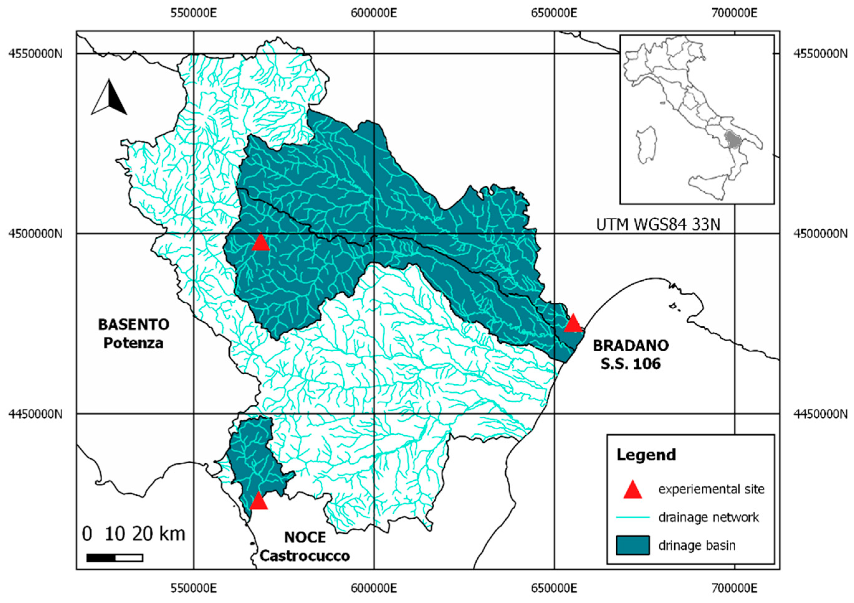
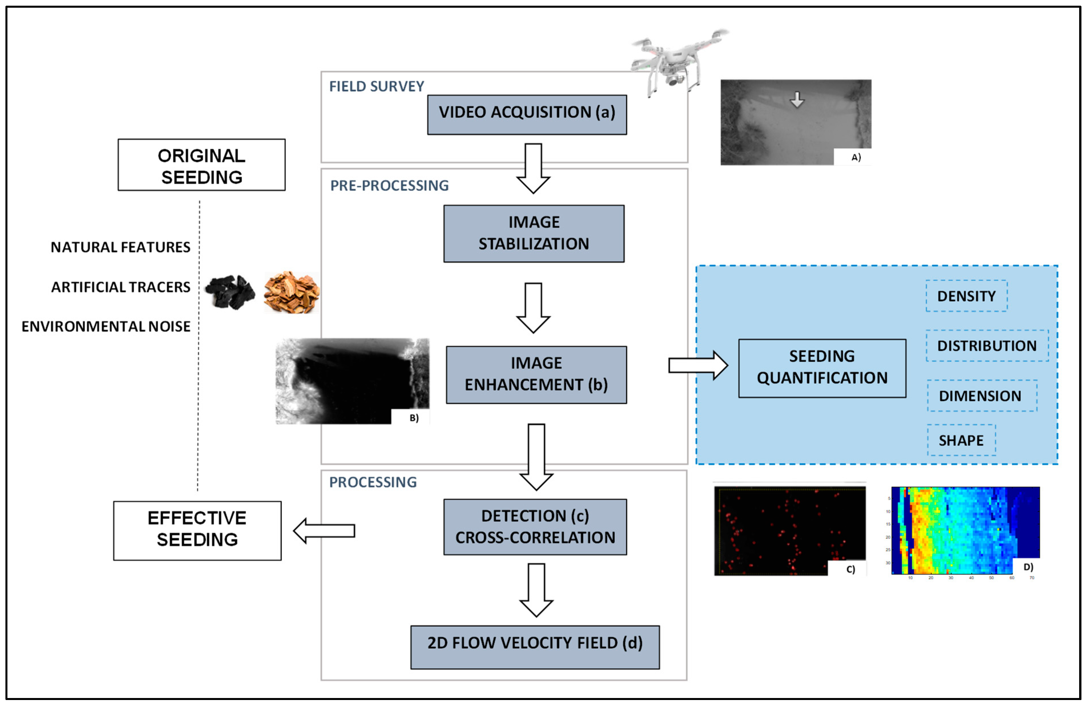
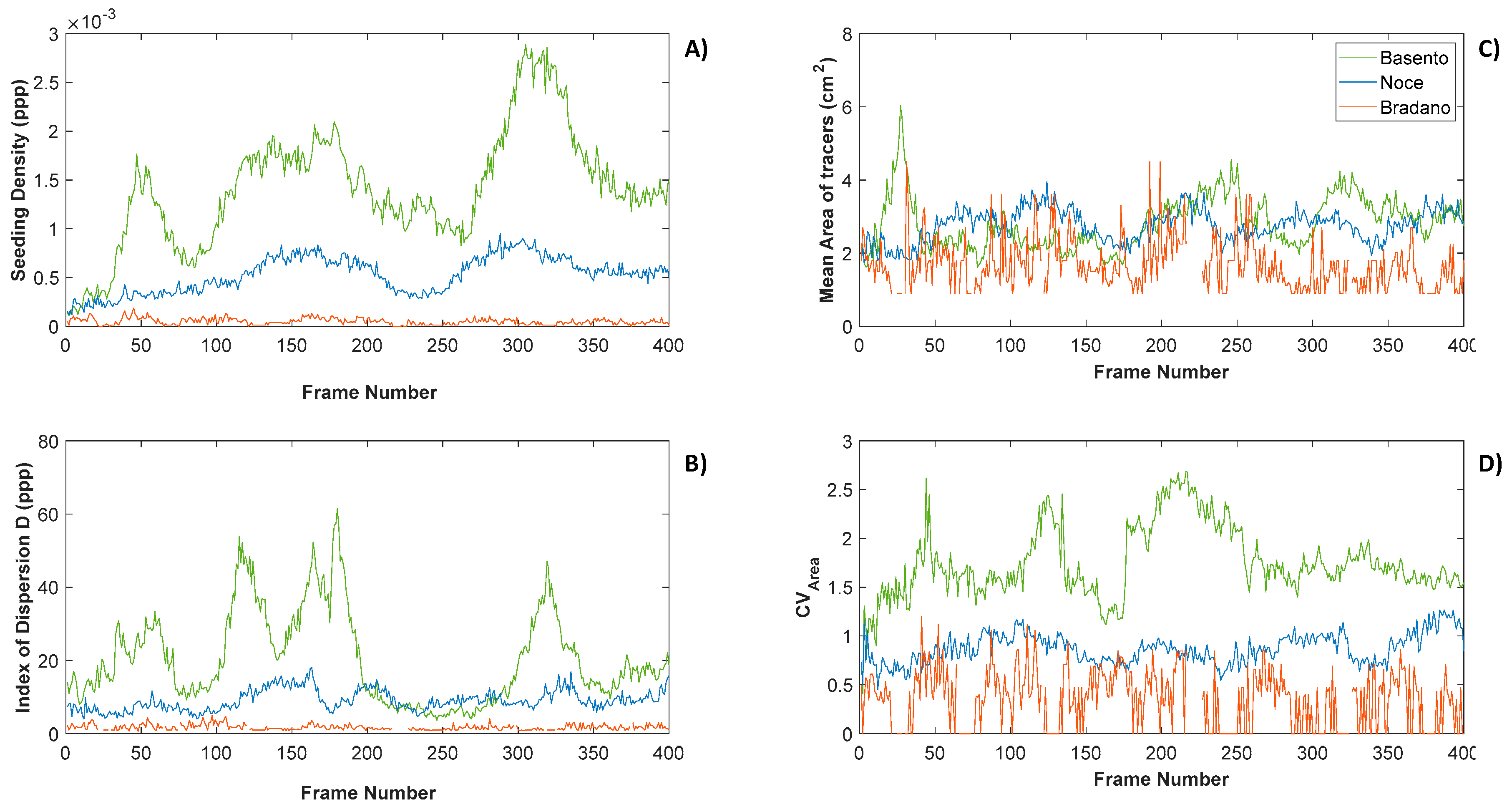
Based on the lack of practical guidelines for image velocimetry analysis based on different seeding properties, we aimed to investigate the accuracy of PTV and LSPIV on three real case studies characterised by different seeding and environmental conditions. To achieve this aim, three metrics were adopted for a preliminary description of seeding characteristics based on calculation of the (i) seeding density, (ii) index of dispersion of tracers, and (iii) coefficient of variation of tracer dimension. These metrics allowed us to describe the spatial and temporal characteristics of seeding during the video acquisition period. The rest of the paper is organised as follows: Section 2 presents the three case studies, field measurements, and video pre-processing procedures. Seeding characterisation using a novel algorithm we recently developed as well as PTV and LSPIV techniques are also briefly introduced. 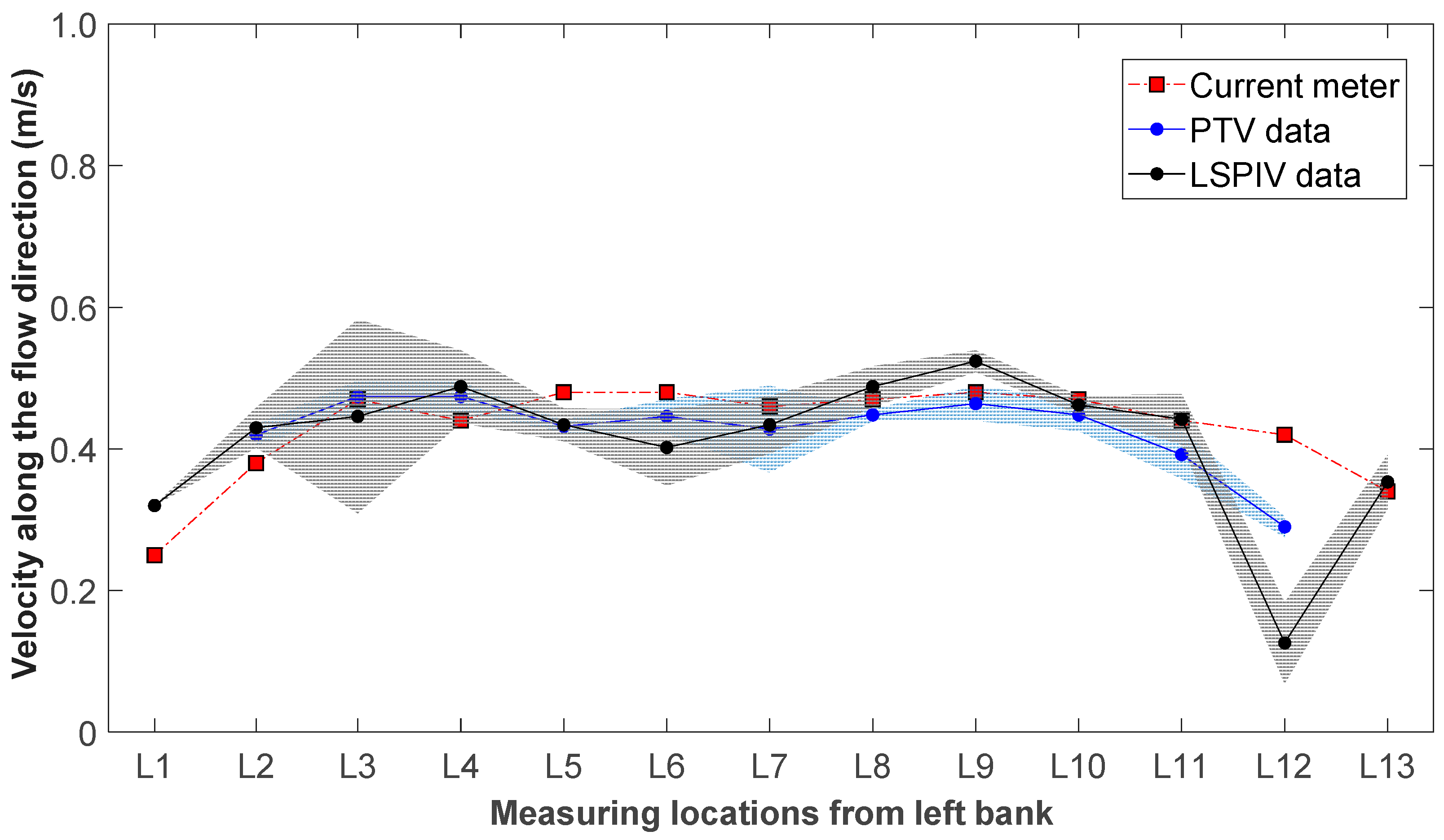Section 3 presents the image velocimetry results compared with reference velocities. The results undergo multiple regression analysis with the aim of identifying the influence of each metric on the associated errors. Conclusions are provided in the final section.

2. Materials and Methods

2.1. Study Area

Three case studies were considered for image velocimetry analysis. Field campaigns were conducted close to three cross-sections at the Noce, Bradano, and Basento Rivers in the Basilicata region of Southern Italy. Figure 1 shows the geographical location of the case studies.

Table 1. Main river flow characteristics in three case studies.

River Section	Secondary Currents	Drainage Area (km2)	Q (m3/s)	Hmax (m)	W (m)	Usmax (m/s)	Usmed (m/s)
Noce River at Castrocucco	No	225	1.70	0.45	14.60	0.48	0.44
Bradano River at SS106	Yes	2581	3.97	0.80	11.40	1.47	0.75
Basento River at Potenza	No	127	0.61	0.38	6.00	0.68	0.40

shows the main hydraulic characteristics of the three case studies: flow conditions, maximum flow depth (H_max), river width (W), maximum surface flow velocity (Us_max), and average surface flow velocity (Us_med). H_max ranged between 0.38 and 0.80 m, and the river width between 6.00 and 14.60 m. Flow conditions at the moment of acquisition differ among case studies, yielding secondary currents. In particular, the Bradano location presented secondary currents in a portion of the cross-sections near the left bank, leading to marked differences in terms of velocity across the cross-section. Figure 2 shows the workflow of surface flow velocity estimation using optical methods. A description of each phase is provided in the following sections.

2.2. Field Measurements

Videos were acquired using a DJI Phantom 3 Pro UAS (DJI, Shenzhen, China) equipped with a Sony Exmor 1/2.3” CMOS (complementary metal oxide semiconductor) sensor. Full high-definition (HD; 1920 × 1080 pixels (px)) RGB videos were captured on the Bradano and Basento Rivers for 103 and 38 s, respectively. An ultra-high-definition (UHD; 3840 × 2160 px) video was acquired on the Noce River for 108 s. All videos were recorded at nadir position in greyscale mode at 24 frames per second (fps) with a duration sufficient to capture a large number of images with appropriate seeding amount and distribution. Different reference objects, useful for image scale calibration and stabilization, were positioned at visible locations on the riverbanks. The calibration factor converting pixels to metres was estimated, considering metric poles with already known dimensions (Figure 3c). The ground sampling distance (GSD) was then computed and the values are reported in

Table 2. Footage properties and reference velocity measurements.

River Section	Equipment	Sensor	RGB Video	Frame Rate	GSD (m/px)	Benchmark
Noce at Castrocucco	DJI Phantom 3 Pro	Sony 1/2.3″ CMOS	3840 × 2160	24	0.009	SEBA F1 current meter
Bradano at SS106	DJI Phantom 3 Pro	Sony 1/2.3″ CMOS	1920 × 1080	24	0.009	SEBA F1 current meter
Basento at Potenza	DJI Phantom 3 Pro	Sony 1/2.3″ CMOS	1920 × 1080	24	0.005	SEBA F1 current meter

(besides other important acquisition variables). Reference velocity measurements were recorded using a current meter in the proximity of the free surface in different locations across the cross-section. The accuracy of the current meter (SEBA F1, SEBA Hydrometrie GmbH & Co, Kaufbeuren, Germany) was within 2% of the measured value [39], which corresponds to 0.001–0.03 m/s for the range of minimum and maximum surface velocities explored in the three case studies. The number of measurement locations was chosen case by case according to the specific conditions, such as cross-section width. In particular, section areas were divided into adjacent locations with 1 m between them for the Noce and Bradano Rivers, and 0.5 m for the Basento River. Each measurement was recorded over a fixed acquisition period of 30 s. The river discharges were evaluated according to ISO-748/1997 [40], using the velocity–area method. The cross-section was divided into panels of equal width and, for each panel, the velocity was measured at 20%, 60%, and 80% of the panel depth.

Seeding materials were manually added to the rivers a few meters upstream of the cross-sections selected for benchmarking purposes. Two operators were used in the process, ensuring proper distribution of seeding material along the entire cross-section. Tracers composed of wood chips and charcoal were selected for extra seeding of regions of interest (ROIs) on clear water (Noce and Basento Rivers) and turbid water (Bradano River) conditions, respectively. On all three rivers, tracers were characterised by irregular shape and homogeneous average dimension (about 2–3 cm).

2.3. Data Pre-Processing

The videos acquired by UAS exhibited a certain degree of motion, mainly caused by wind-induced turbulence and vibrations. The occurrence of these movements was outside the limits of the self-stabilizing camera (gimbal). Therefore, to improve the velocity estimations, video captured with UASs was first stabilised using an automatic feature selection method that identifies features in frame pairs, matching them to compute possible values of translation and rotation. The features from accelerated segment test (FAST) detection algorithm was applied to identify features on an ad-hoc ROI [12,41]. To improve the feature matching accuracy, at each step, the method utilises the random sample consensus (RANSAC) filter for unacceptable correspondence [16,42]. Applying the stabilisation algorithm for the case studies allowed us to reduce the effects of camera movements throughout the entire video. Planimetric errors considering differences in translation and rotation were computed, taking the first frame as the reference target. On average, the reduction due to the stabilisation process ranged from 43 to 7 px, from 48 to 5 px, and from 64 to 7 px for the Noce, Bradano and Basento Rivers, respectively, for a reduction of around 85–90% of the original video movement. The stabilisation algorithm does not require ground control points (GCPs) to be applied. Consequently, it detects features automatically and the stabilisation process is therefore a viable alternative for inexperienced users.

The Basento and Noce Rivers have low flow conditions, leading to subsampling of the original video from 24 to 12 fps. In contrast, for the Bradano River, we used the original rate of 24 fps. The appropriate fps was chosen to ensure frame-by-frame displacement larger than particle dimension [34] and to minimise the effects of camera movement between frame pairs on the calculation of surface velocities.

All case studies were acquired in greyscale and pre-processed using contrast stretching techniques to enhance the visibility of the artificial tracers against the background. For this purpose, the GNU Image Manipulation Program (GIMP) was used, adjusting brightness and contrast. Image pre-processing included a manual contrast stretch conducted with the use of GIMP manipulation software (GNU General Public License). The images were processed using the threshold tool in batch mode. Each frame was transformed into a black and white image adopting a digital number (DN) threshold of 200. This procedure allowed a large amount of noise caused by external reflections to be eliminated, improving the number of tracers identified and cross-correlated in the ROI. Figure 3 shows the original frames, the ROI (red squares) after pre-processing, and the location of reference velocity measurements.

2.4. Seeding Characterisation

The use of enhanced frames allowed us to emphasise the appearance of features with respect to the background, enabling the extraction of relevant information about the seeding characteristics of the flow. A detection algorithm was implemented to compute the seeding density in particles per pixel (ppp), the dimensions of features, and their spatial variance. The detection algorithm is an ad-hoc piece of code we wrote to characterise features for image-velocimetry purposes. Consequently, the number of features, their relative positions, and associated areas were identified using it. This enabled the characterisation of the seeding properties and metrics introduced in this paper a frame-by-frame basis, even though shapes and dimensions of the tracers varied considerably. The feature detection relies on an automated process to detect and describe features in the footage frames. These features can be local corners, blobs, or regions of uniform intensity and were saved and postprocessed to derive the metrics used in this paper. MATLAB R2019a (MathWorks, Natick, MA, USA) was used for this purpose. Original seeding is characterised by added tracers (extra seeding), environmental noise (e.g., illumination, shadows and ripples), and natural tracers transiting onto the flow surface. Overall, the equivalent diameter of actual seeding inside the ROI was estimated as 1.5 and 2 cm at Bradano and Noce Rivers, respectively; on the Basento River, this value was about 2.7 cm. Figure 4 depicts examples of the identification of features and a zoom-in inside the ROI. As can be seen, the algorithm was able to correctly identify the features, even if they had different shapes and dimensions.

Figure 5 provides a comprehensive overview of the seeding behaviour during an arbitrarily selected acquisition period for each of the three case studies. Since they all had different durations, the maximum number of frames was expected to be diverse. Nevertheless, we decided to make this value uniform, setting it arbitrarily to 400 images. Figure 5a,b present the seeding density and mean area of tracers over time. The mean area of features showed similar behaviour and order of magnitude over time, with values between 1.5 and 4 cm² for the three case studies analysed.

The change in the spatial distribution of features for the ROI was quantified through the spatial dispersion index D (= Var(N)/E(N), where Var(N) and E(N) are spatial variance and mean value of the number of tracers N, respectively, computed on subsectors of 100 × 100 pixels), which is a metric used to quantify the level of aggregation/dispersion of tracers. D = 1 means features follow a Poisson distribution, whereas D < 1 and D > 1 indicate they follow an over- and under-dispersed spatial distribution, respectively. Figure 5c shows the dispersion index as a function of the number of frames for each case study. In particular, the Basento River presented the highest values of aggregation, with D > 40 during recording periods. The Bradano River had the lowest and most stable values of D, with none above three. The homogeneity of tracer shapes was quantified using the coefficient of variation of tracer areas (CV_Area), which is presented in Figure 5d. The Basento River had the highest values of CV, leading to heterogeneity in terms of feature shapes.

Table 3. Average seeding characteristics.

River Section	Tracers	Average Feature Dimension (Equivalent Diameter in cm)	Average Seeding Density (ppp)	Average Dispersion Index (ppp)	Average CVArea
Noce River at Castrocucco	Woodchip	1.98	5.28 × 10−4	9.09	0.87
Bradano River at SS106	Charcoal	1.53	4.99 × 10−5	1.72	0.35
Basento River at Potenza	Woodchip	2.68	1.40 × 10−3	20.37	1.76

presents an overview of the average values of key variables related to tracers transiting the ROI.

2.5. Image Velocimetry

2.5.1. Data Processing

Image velocimetry techniques were applied to five sets of images to measure the accuracy of surface velocity estimation in changing seeding conditions. In this context, the length of the acquisition was fundamental for further analysis. The number of images considered in each frame window was decided arbitrarily but consistent with other research available in the literature [12,20,23,24]. For the Bradano River, frame windows 1–5 (named FW1–FW5) were defined as 1 to 200, 51 to 250, 101 to 300, 151 to 350, and 201 to 400 frames, respectively. For the Noce and Basento Rivers, due to the video resampling to 12 fps, frame windows were defined as 1 to 100, 26 to 125, 51 to 150, 76 to 175, and 101 to 200, respectively.

For the analysis, PIVlab [43] and PTVlab [34] were used to estimate the surface flow velocity on the three rivers. The PTV technique was implemented using cross-correlation by interrogation area (IA). Specifically, the IA was set to 25 px, the cross-correlation threshold as 0.4, and the neighbour similarity percentage to 20%. Particles were detected through correlation with a Gaussian mask of 4 px in diameter and 70 px in maximum intensity. These detection parameters allowed consideration of the high variability of the feature dimensions in the Basento River, mainly characterised by a lower GSD with respect to the others. The correlation threshold was set to 0.5. The LSPIV algorithm was applied using fast Fourier transform (FFT) with three-pass standard correlation and IA sizes of 128 × 64, 64 × 32, and 32 × 16 px. The 2 × 3-point Gauss sub-pixel estimator was applied.

2.5.2. Comparison with Reference Velocities

The velocities were compared using the current meter considering only the component of velocity in the flow direction (U). For PTV and LSPIV analysis, velocity values of each node represent the average of velocity estimated in a square with sides of 0.30 m centred on the measured point [20]. The accuracy of the different image velocimetry algorithms was evaluated by calculating the percent error (ε), defined as follows:

$$\mathsf{\epsilon }=\left(\left({\mathrm{U}}_{\mathrm{c}}-{\mathrm{U}}_{\mathrm{m}}\right)/{\mathrm{U}}_{\mathrm{m}}\right)\times 100,$$

(1)

where U_m represents the velocity measured with the current meter and U_c is the average computed velocity obtained by the LSPIV or PTV method.

For each frame sequence, the root mean square error (RMSE) values between PTV and LSPIV results and the current meter data were also calculated:

$$\mathrm{RMSE}=\sqrt{1/\mathrm{n}{{\displaystyle \sum }}_{1=1}^{\mathrm{n}}{\left({\mathrm{U}}_{\mathrm{ci}}-{\mathrm{U}}_{\mathrm{mi}}\right)}^2}.$$

(2)

3. Results

3.1. Image Velocimetry Results

3.1.1. Noce River

Image velocimetry techniques were applied in the frame windows defined in Section 2.5.1. The average seeding density was estimated as 4.4 × 10⁻⁴, 4.7 × 10⁻⁴, 5.3 × 10⁻⁴, 5.8 × 10⁻⁴, and 5.4 × 10⁻⁴ ppp for FW1, FW2, FW3, FW4, and FW5, respectively. Therefore, the seeding density presented a 19% increase from FW1 to FW5. The use of PTV showed that the cross-correlation process was considerably affected by different environmental conditions (water reflection and background noise), deteriorating the matching and tracking process. The number of tracers detected on the configurations was respectively 69, 73, 84, 91, and 85 and the number of tracers effectively cross-correlated was, on average, 29, 32, 38, 40, and 39, respectively. Consequently, the seeding density considered in the analysis was around 44% of the original (i.e., an estimated reduction of 56%). The information on tracers detected and cross-correlated for each image pair is a piece of information available in the MATLAB command window during PTVLab software execution.

Table 4. Average seeding characteristics of frame sequences with root mean square error (RMSE) computed for different techniques. Percentage of locations with estimated value using image velocimetry techniques shown in parentheses. FW, frame window; PTV, particle tracking velocimetry; LSPIV, large-scale particle image velocimetry.

Description	Dimension	FW1	FW2	FW3	FW4	FW5
Frames		1–100	26–125	51–150	76–175	101–200
Average particles	number	69	73	84	91	85
Average seeding density	ppp	4.4 × 10−4	4.7 × 10−4	5.3 × 10−4	5.8 × 10−4	5.4 × 10−4
Average particle detected (PTV)	number	29	32	38	40	39
Effective seeding density (PTV)	ppp	1.9 × 10−4	2.0 × 10−4	2.4 × 10−4	2.5 × 10−4	2.5 × 10−4
RMSE-PTV	m/s	0.056 (77%)	0.053 (85%)	0.062 (85%)	0.049 (85%)	0.051 (85%)
RMSE-LSPIV		0.117 (85%)	0.092 (85%)	0.110 (92%)	0.093 (100%)	0.116 (92%)

shows the principal seeding characteristics considering the different sets of images and RMSE values of estimated surface flow velocities using the PTV and LSPIV algorithms. The number of reference measurement locations of the computed velocities using PTV and LSPIV (in pecentual) is shown in parentheses in Table 4. Overall, an increasing number of computed locations from FW1 to FW5 was observed. At FW4, LSPIV was able to reconstruct 100% of the reference velocity locations, whereas PTV was able to reconstruct only 85%. Figure 6a,b show the averaged surface velocity maps calculated using the PTV and LSPIV algorithms for frame window FW4. Surface velocity values calculated with PTV appeared less noisy in the whole cross-section compared with LSPIV, which seemed to be more influenced by environmental factors (sunlight reflection and background) during the acquisition time.

Table A1. PTV and LSPIV results for each location compared to reference measurements on the Noce River.

Location	U (m/s)	PTVVelocity(m/s)					PTVPercent Error(%)
		FW1	FW2	FW3	FW4	FW5	FW1	FW2	FW3	FW4	FW5
L1	0.25	n/a	n/a	n/a	n/a	n/a	n/a	n/a	n/a	n/a	n/a
L2	0.38	0.43	0.44	0.41	0.41	0.41	13.98	15.70	7.90	8.89	9.34
L3	0.47	0.51	0.48	0.47	0.46	0.45	7.04	1.20	0.25	−k3.28	−5.13
L4	0.44	0.45	0.50	0.49	0.47	0.46	2.91	13.85	11.18	7.04	5.33
L5	0.48	0.44	0.44	0.43	0.43	0.42	−8.06	−8.88	−11.07	−10.80	−12.37
L6	0.48	0.48	0.46	0.42	0.44	0.43	−0.59	−4.46	−13.87	–9.57	−11.59
L7	0.46	0.33	0.41	0.45	0.47	0.48	−29.07	−11.63	−2.71	2.78	4.33
L8	0.47	0.44	0.45	0.44	0.46	0.45	−6.52	−3.76	−6.77	–3.34	−3.77
L9	0.48	0.43	0.47	0.48	0.49	0.45	−11.27	−2.54	0.14	0.53	−5.91
L10	0.47	0.41	0.45	0.46	0.47	0.45	−12.97	−4.92	−3.60	−0.82	−4.15
L11	0.44	0.45	0.38	0.36	0.39	0.38	1.64	−14.42	−18.28	−11.55	−13.10
L12	0.42	n/a	0.30	0.27	0.29	0.30	n/a	−27.78	−36.26	−30.80	−28.03
L13	0.34	n/a	n/a	n/a	n/a	n/a	n/a	n/a	n/a	n/a	n/a
Location	U (m/s)	LSPIVVelocity(m/s)					LSPIVPercent Error(%)
		FW1	FW2	FW3	FW4	FW5	FW1	FW2	FW3	FW4	FW5
L1	0.25	n/a	n/a	n/a	0.32	n/a	n/a	n/a	n/a	27.59	n/a
L2	0.38	0.48	0.42	0.42	0.41	0.42	27.47	12.99	10.50	7.75	10.40
L3	0.47	0.38	0.64	0.27	0.45	0.49	–19.05	36.17	–42.75	–3.75	4.19
L4	0.44	0.48	0.43	0.57	0.49	0.47	10.09	–2.84	30.43	10.64	6.03
L5	0.48	0.47	0.42	0.43	0.41	0.44	–2.45	–13.18	–11.01	–16.02	–9.51
L6	0.48	0.40	0.49	0.35	0.40	0.37	–16.87	1.25	–26.54	–18.16	–22.51
L7	0.46	0.38	0.43	0.45	0.49	0.42	–18.73	–7.20	–3.45	6.47	–9.44
L8	0.47	0.51	0.49	0.44	0.49	0.51	7.89	3.79	–7.01	3.32	8.20
L9	0.48	0.51	0.52	0.52	0.55	0.52	6.37	7.69	6.77	13.65	8.45
L10	0.47	0.47	0.45	0.48	0.45	0.46	–0.71	–4.64	2.21	–3.97	–1.81
L11	0.44	0.49	0.47	0.42	0.41	0.42	11.53	5.99	–4.98	–7.37	–5.29
L12	0.42	0.09	0.19	0.17	0.13	0.05	–79.36	–55.19	–58.80	–68.80	–88.64
L13	0.34	n/a	n/a	0.37	0.31	0.38	n/a	n/a	8.40	–9.32	10.51

(see Appendix A) shows the surface velocities and percent errors (%) calculated for both image velocimetry techniques for each frame window considered in the analysis. The locations with very low seeding density had uncertain results or no estimation of velocity. This is reasonable, since without seeding, it was not possible to perform matching and tracking of features. This was the case for L1, L12, and L13 (from the left bank), which presented very low seeding densities during the whole period of analysis (PTV). Difficulties in computing surface flow velocity under those conditions arose, as shown in Table A1 (n/a values). Increasing the seeding and distribution of tracers from FW1 to FW5 allowed the computation of the surface flow velocity in different portions of the river cross-section. Figure 7 provides a visual comparison between the average surface velocities measured with a current meter and computed with the LSPIV and PTV algorithms. Shaded regions represent calculated standard deviations considering the different frame windows. Both image-based approaches correctly captured the velocity in the centre of the cross-section, with lower effectiveness near the banks. LSPIV generally showed higher standard deviations for the results compared with PTV at the different reference locations.

3.1.2. Bradano River

PTV and LSPIV image velocimetry techniques were applied to the five frame windows defined by the number of frames from 1 to 400. The average seeding density was estimated as 6.8 × 10⁻⁵, 5.5 × 10⁻⁵, 6.7 × 10⁻⁵, 7.6 × 10⁻⁵, and 7.8 × 10⁻⁵ ppp for FW1, FW2, FW3, FW4, and FW5, respectively. Therefore, the seeding density was almost constant from FW1 to FW5. The PTV algorithm detected five, four, five, six, and six tracers on FW1, FW2, FW3, FW4, and FW5, respectively, on average. From those, only four tracers on average were effectively cross-correlated at the matching process. Consequently, the effective seeding considered in the analysis was reduced, and its value was around 81% of the original.

Table 5. Average seeding characteristics of frame sequences with indication of RMSE computed with different techniques. Percentage of locations with estimated value using image velocimetry techniques shown in parentheses.

Description	Dimension	FW1	FW2	FW3	FW4	FW5
Frames		1–200	51–250	101–300	151–350	201–400
Average particles	number	5	4	5	6	6
Average seeding density	ppp	6.8 × 10−5	5.5 × 10−5	6.7 × 10−5	7.6 × 10−5	7.8 × 10−5
Average particle detected (PTV)	number	4	3	4	4	4
Effective seeding density (PTV)	ppp	5.3 × 10−5	4.6 × 10−5	5.3 × 10−5	5.9 × 10−5	6.0 × 10−5
RMSE-PTV	m/s	0.209 (43%)	0.144 (29%)	0.075 (43%)	0.070 (57%)	0.040 (71%)
RME-LSPIV		0.151 (71%)	0.040 (71%)	0.066 (71%)	0.066 (71%)	0.056 (71%)

shows the principal seeding characteristics and RMSE values of estimated surface flow velocities employing the PTV and LSPIV algorithms. The results showed that LSPIV allowed the surface velocity calculation to cover more than 70% of the measurement locations in all frame windows considered in the analysis. PTV covered the same number of measurement locations only if FW5 was considered, improving RMSE results with respect to LSPIV. Figure 8a,b show the representative averaged surface velocity maps calculated using the PTV and LSPIV algorithms for frame window FW5. The surface velocity map of LSPIV is more complete compared to that of PTV. This can be explained by LSPIV’s ability to identify and track other natural features transiting on the water surface (ripples and waves).

Figure 9 and

Table A2. PTV and LSPIV results for each location compared to reference measurements on the Bradano River.

Location	U (m/s)	PTVVelocity(m/s)					PTVPercent Error(%)
		FW1	FW2	FW3	FW4	FW5	FW1	FW2	FW3	FW4	FW5
L1	0.84	n/a	n/a	n/a	n/a	n/a	n/a	n/a	n/a	n/a	n/a
L2	1.48	1.18	n/a	n/a	n/a	1.46	−20.05	n/a	n/a	n/a	–1.08
L3	1.04	0.84	0.86	0.96	0.96	0.98	−19.31	−17.11	−7.47	−7.76	–5.74
L4	0.77	0.83	0.87	0.87	0.87	0.81	7.88	12.97	12.67	12.78	5.48
L5	0.53	n/a	n/a	0.49	0.49	0.49	n/a	n/a	−6.65	−6.82	–6.59
L6	0.43	n/a	n/a	n/a	0.48	0.39	n/a	n/a	n/a	10.88	–8.26
L7	0.63	n/a	n/a	n/a	n/a	n/a	n/a	n/a	n/a	n/a	n/a
Location	U (m/s)	LSPIVVelocity(m/s)					LSPIVPercent Error(%)
		FW1	FW2	FW3	FW4	FW5	FW1	FW2	FW3	FW4	FW5
L1	0.84	n/a	n/a	n/a	n/a	n/a	n/a	n/a	n/a	n/a	n/a
L2	1.48	1.20	1.47	1.42	1.42	1.38	−18.92	–0.64	–3.83	–3.83	–6.60
L3	1.04	0.86	0.99	0.93	0.93	0.99	−17.07	–4.79	−10.06	–10.06	–4.39
L4	0.77	0.83	0.79	0.76	0.76	0.74	7.05	2.27	−1.08	–1.08	–3.93
L5	0.53	0.56	0.56	0.55	0.55	0.57	5.96	7.23	5.15	5.15	8.42
L6	0.43	0.46	0.49	0.51	0.51	0.47	6.63	14.19	19.24	19.24	8.52
L7	0.63	n/a	n/a	n/a	n/a	n/a	n/a	n/a	n/a	n/a	n/a

(see Appendix A) present the PTV and LSPIV results for each frame window described previously. L1 and L7 had no seeding in all frames analysed. Consequently, they had no estimation of surface flow velocity on the considered frame windows. At locations L2, L5, and L6, PTV showed velocity estimates only for some frame windows due to the low number of tracked tracers. At the same locations, LSPIV provided surface velocity estimates. LSPIV does not work well under low seeding densities; thus, it is expected that PTV outperforms LSPIV in those conditions. However, even though the seeding density was low, average image velocimetry values were in close agreement with current meter measurements (between 5% and 20%).

3.1.3. Basento River

Image velocimetry techniques were applied to the five frame windows defined by the number of frames from 1 to 200. The average seeding density estimated using the PTV algorithm was 1.9 × 10⁻⁴, 3.5 × 10⁻⁴, 4.5 × 10⁻⁴, 4.5 × 10⁻⁴, and 4.6 × 10⁻⁴ ppp for FW1, FW2, FW3, FW4, and FW5, respectively. Therefore, the seeding density increased from FW1 to FW3, then from FW3 to FW5, it was almost constant. Local environmental conditions such as low flow depth, clear water, visualisation of bed material, and tracers with different shapes and dimensions led to a reduction in the original seeding density considered in the analysis (effective seeding). For the PTV algorithm, this reduction was quantified as 81%; consequently, only the residual 19% was effectively used for tracking features, as outlined in

Table 6. Average seeding characteristics of frame sequences with RMSE computed with different techniques. Percentage of locations with estimated value using image velocimetry techniques shown in parentheses.

Description	Dimension	FW1	FW2	FW3	FW4	FW5
Frames		1–100	26–125	151–250	176–275	101–200
Average particles	number	20	38	48	48	49
Average seeding density	ppp	1.9 × 10−4	3.5 × 10−4	4.5 × 10−4	4.5 × 10−4	4.6 × 10−4
Average particles detected (PTV)	number	5	7	9	9	9
Effective seeding density (PTV)	ppp	5.0 × 10−5	6.6 × 10−5	8.0 × 10−5	8.3 × 10−5	8.5 × 10−5
RMSE-PTV	m/s	0.159 (64%)	0.168 (82%)	0.138 (82%)	0.163 (73%)	0.142 (73%)
RMSE-LSPIV		0.140 (91%)	0.117 (82%)	0.116 (82%)	0.130 (91%)	0.123 (91%)

and Figure 10, which show that only 64% of the locations were able to compute PTV velocity.

Figure 11 and

Table A3. PTV and LSPIV results for each location compared to reference measurements on the Basento River.

Location	U (m/s)	PTVVelocity(m/s)					PTVPercent Error(%)
		FW1	FW2	FW3	FW4	FW5	FW1	FW2	FW3	FW4	FW5
L1	0.05	n/a	n/a	n/a	n/a	n/a	n/a	n/a	n/a	n/a	n/a
L2	0.17	n/a	n/a	n/a	n/a	n/a	n/a	n/a	n/a	n/a	n/a
L3	0.43	0.48	0.48	0.47	0.45	0.44	12.21	12.34	8.40	5.32	2.12
L4	0.58	0.55	0.43	0.50	0.47	0.46	–5.33	−25.31	–14.02	–18.13	–20.39
L5	0.29	0.20	0.22	0.22	0.23	0.23	–29.97	−23.65	–24.05	–20.52	–20.56
L6	0.29	0.30	0.33	0.32	0.34	0.34	4.62	12.20	10.00	18.27	16.04
L7	0.61	0.31	0.35	0.50	0.39	0.47	–49.82	−42.20	–17.94	−36.30	−23.18
L8	0.68	n/a	0.39	0.39	0.38	0.39	n/a	−42.79	–42.79	−43.70	−42.69
L9	0.54	n/a	0.47	0.47	n/a	n/a	n/a	−12.46	–12.46	n/a	n/a
L10	0.50	0.40	0.40	0.38	0.37	0.49	–21.42	−21.26	–25.06	−27.21	−3.63
L11	0.43	0.18	0.19	0.23	0.23	0.23	–57.58	−55.55	–47.26	−46.16	−45.52
Location	U (m/s)	LSPIVVelocity(m/s)					LSPIVPercent Error(%)
		FW1	FW2	FW3	FW4	FW5	FW1	FW2	FW3	FW4	FW5
L1	0.05	n/a	n/a	n/a	n/a	n/a	n/a	n/a	n/a	n/a	n/a
L2	0.17	0.35	n/a	n/a	0.13	0.17	103.61	n/a	n/a	–26.51	–2.78
L3	0.43	0.50	0.49	0.49	0.43	0.47	17.24	12.95	16.75	0.51	10.07
L4	0.58	0.46	0.42	0.42	0.42	0.41	–20.67	–27.37	–24.50	–26.75	–29.08
L5	0.29	0.15	0.15	0.15	0.17	0.20	–47.93	–49.37	–20.27	–41.35	–30.07
L6	0.29	0.36	0.34	0.34	0.35	0.33	24.25	18.07	23.13	20.07	12.77
L7	0.61	0.58	0.58	0.58	0.53	0.55	–4.78	–4.88	–5.57	–13.01	–10.71
L8	0.68	0.47	0.46	0.46	0.46	0.48	–29.79	–31.57	–27.42	–31.24	–28.43
L9	0.54	0.51	0.49	0.49	0.49	0.52	–4.11	–8.11	–3.75	–8.67	–2.71
L10	0.50	0.38	0.39	0.39	0.37	0.39	–24.85	–22.63	–19.95	–26.19	–22.64
L11	0.43	0.18	0.33	0.33	0.19	0.19	–58.05	–23.80	–47.75	–54.97	–56.07

(see Appendix A) show the computed velocity results for each frame window chosen for analysis. In particular, PTV was not able to compute velocities across the entire cross-section, whereas LSPIV computed them on all point measurements. This can be explained by LSPIV involving other tracking surface features, such as ripples and colour differences in the water surface. Notably, the tracers were scarce for locations closer to the riverbanks (L1 and L2), putting the image velocimetry algorithms under critical stress. In this case study, both techniques tended to underestimate surface flow velocity, especially on the right side of the cross-section. We observed that for all frame windows analysed, LSPIV had lower RMSE values than PTV.

3.2. Multiple Regression Analysis

Multiple linear regression analysis was performed to statistically evaluate the significance of the investigated seeding parameters on the performance of PTV and LSPIV. The variables under consideration were the same ones characterised in this study: seeding density, index of dispersion, and spatial variance of tracer dimension. For each case study, the average of absolute percent errors for each frame window was computed and correlated. Seeding characteristics were standardised since the weight of each variable was of special interest. The following relationship was then considered for modelling purposes:

ε_m = C₁(ρ/max(ρ)) + C₂(D/max(D)) + C₃(CV_Area/max(CV_Area)),

(3)

where ε_m is the absolute percent error, ρ is the seeding density, D is the dispersion index, CV_Area is the coefficient of variation of tracer area, and C₁, C₂, and C₃ are the multiple regression coefficients.

The results of the analysis, summarised in

Table 7. Parameters and statistics of multiple linear regression analysis.

Algorithm	C1	C2	C3	R2	p-Value
PTV	–14.6932	2.9118	35.7002	0.8001	0.0001
LSPIV	–18.5738	21.0869	26.0480	0.8083	0.0000

, showed that the three metrics had similar significance in the derived multilinear regression. A negative correlation was found between absolute percent error and seeding density. This means that increasing the seeding density resulted in fewer errors. The velocimetry errors showed a positive correlation with the dispersion index and coefficient of variation of tracer area. The coefficient of variation of particle size appeared to have a slightly greater impact on PTV with respect to the other terms, and the dispersion coefficient had significantly less impact on the regression of PTV with respect to LSPIV. This last result was somewhat influenced by the algorithm, which restricts the area of investigation to the portion of the domain with particles. Therefore, PTV is less affected by particle dispersion. The coefficient of determination (R²) and statistical significance (p-value) were evaluated as measures of fitting performance. For both techniques, the values were R² = ~0.80 and p < 0.001 (Table 7). Figure 12 shows the errors predicted by the multiple regression analysis and those observed with the use of PTV and LSPIV.

4. Discussion

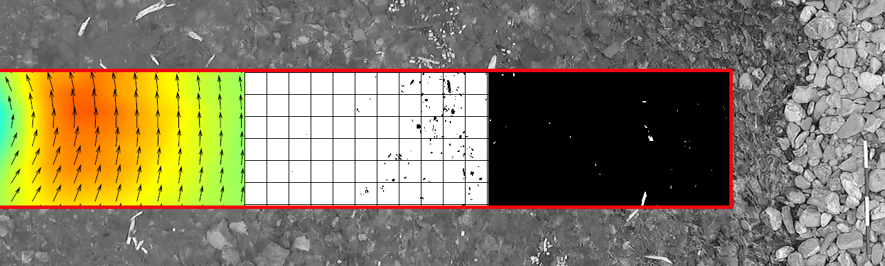
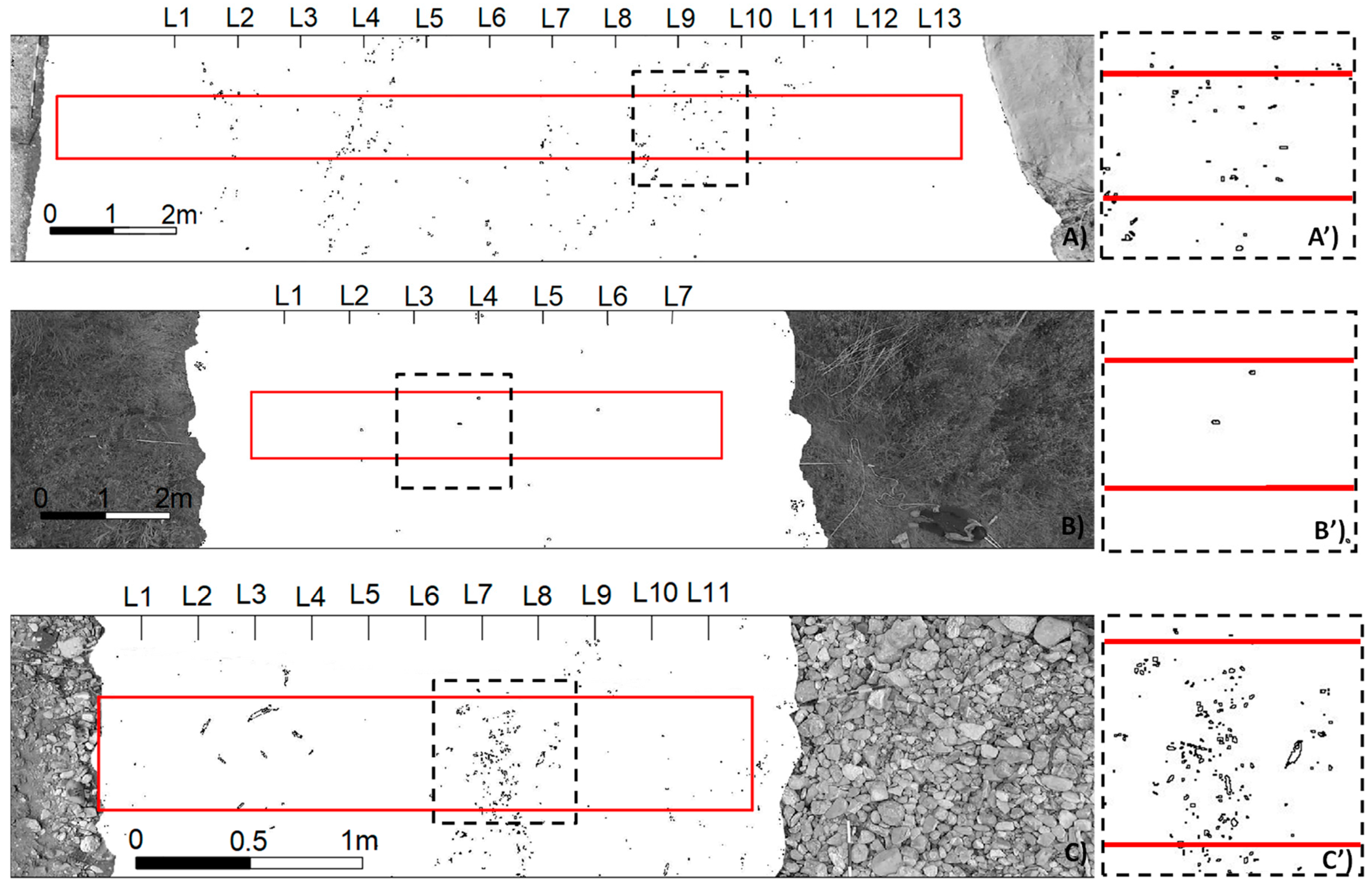
The number, distribution, and characteristics of features on the surface of water are crucial factors for obtaining accurate PTV and LSPIV results. Seeding can be represented by flow features (e.g., ripples), natural objects transiting in the field of view, or artificial floaters. Generally, in field applications, the shape and dimension of floating material can be non-uniform and the spatial distribution of features inhomogeneous in the whole cross-section. Actual seeding in field conditions does not necessarily represent the effective seeding that is used for the application of optical techniques. This is evidenced by the process of detecting and matching features between image pairs. Noise due to environmental conditions, such as illumination or shadows, can strongly influence the quantification of effective seeding. Low seeding due to a lack of tracers or matching issues generally lead to an incomplete surface velocity field or unreliable results. However, in the pre-processing phase, the original seeding can be maximised using techniques to emphasise the contrast between tracers and water background. This step is essential for facilitating particle detection and cross-correlation. In turn, filters can be applied in a post-processing phase to improve the reliability of cross-correlation results in deleting spurious vectors.

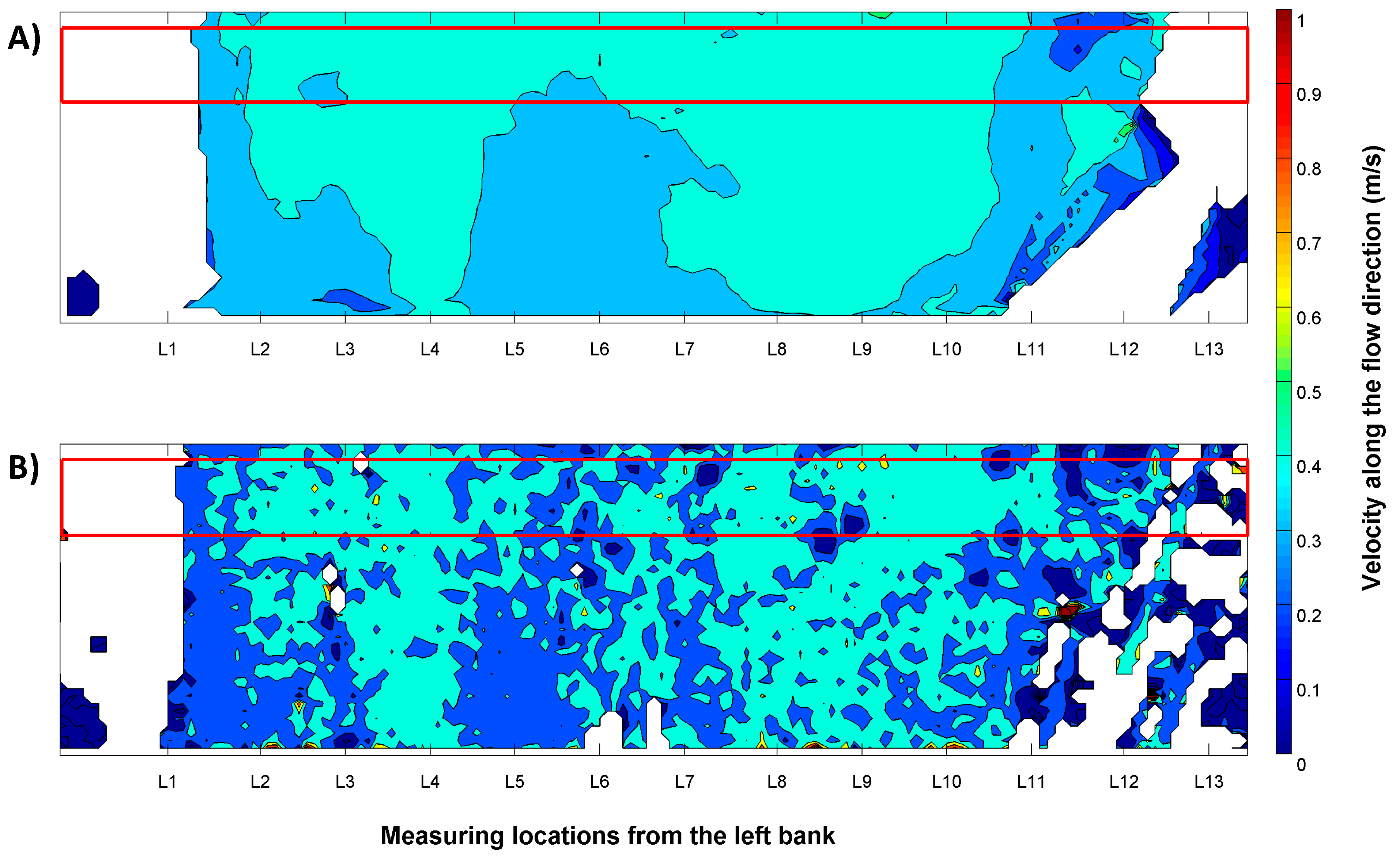
In this work, three metrics were defined and implemented to quantify the seeding behaviour in the pre-processing phase: seeding density in ppp, the dispersion index, and the coefficient of variation of tracer area. They were applied in three field case studies characterised by different environmental conditions and seeding characteristics. LSPIV and PTV techniques were applied to pre-processed images to maximise the contrast between particles and background, without any filter to isolate and remove inaccurate vectors (outliers).

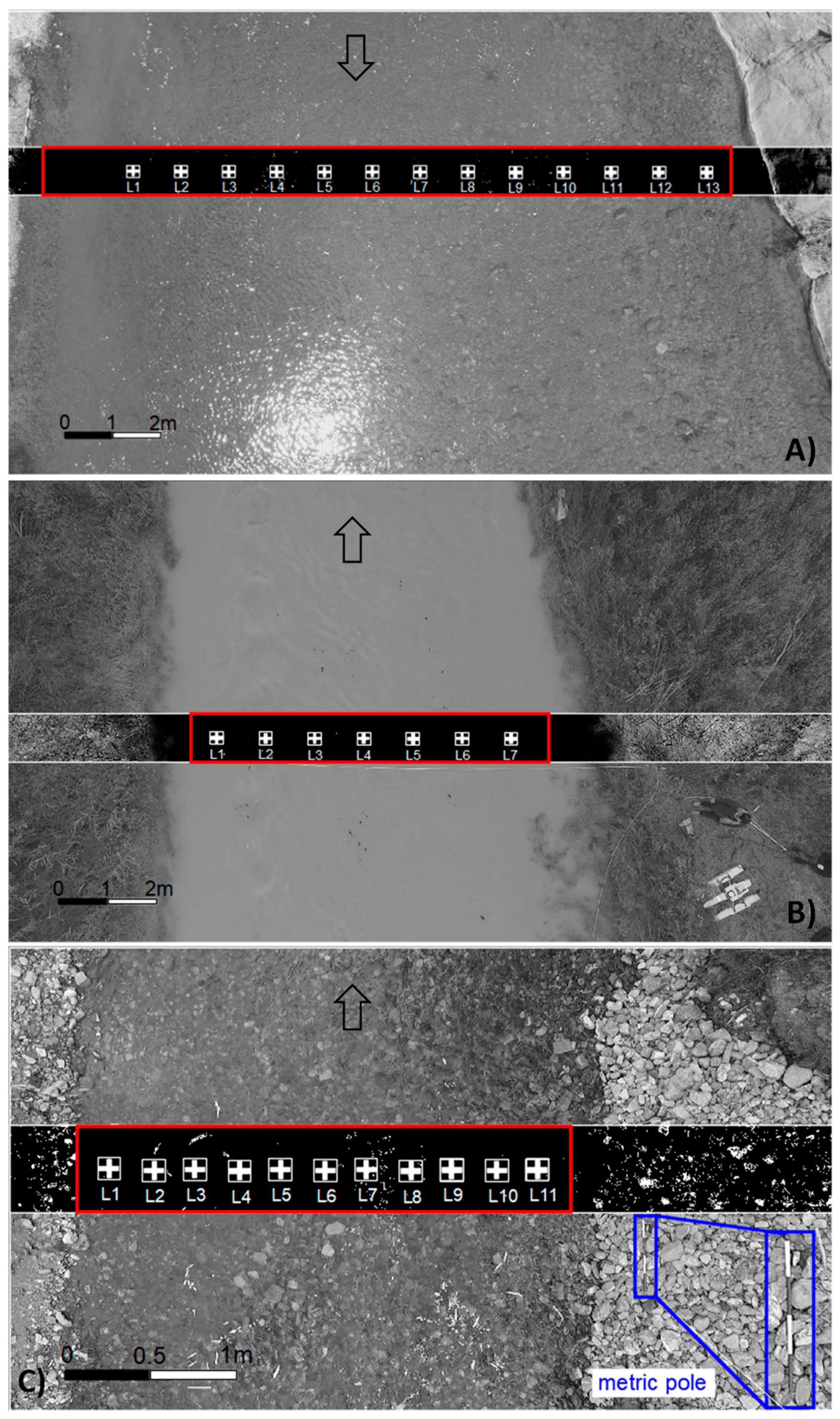
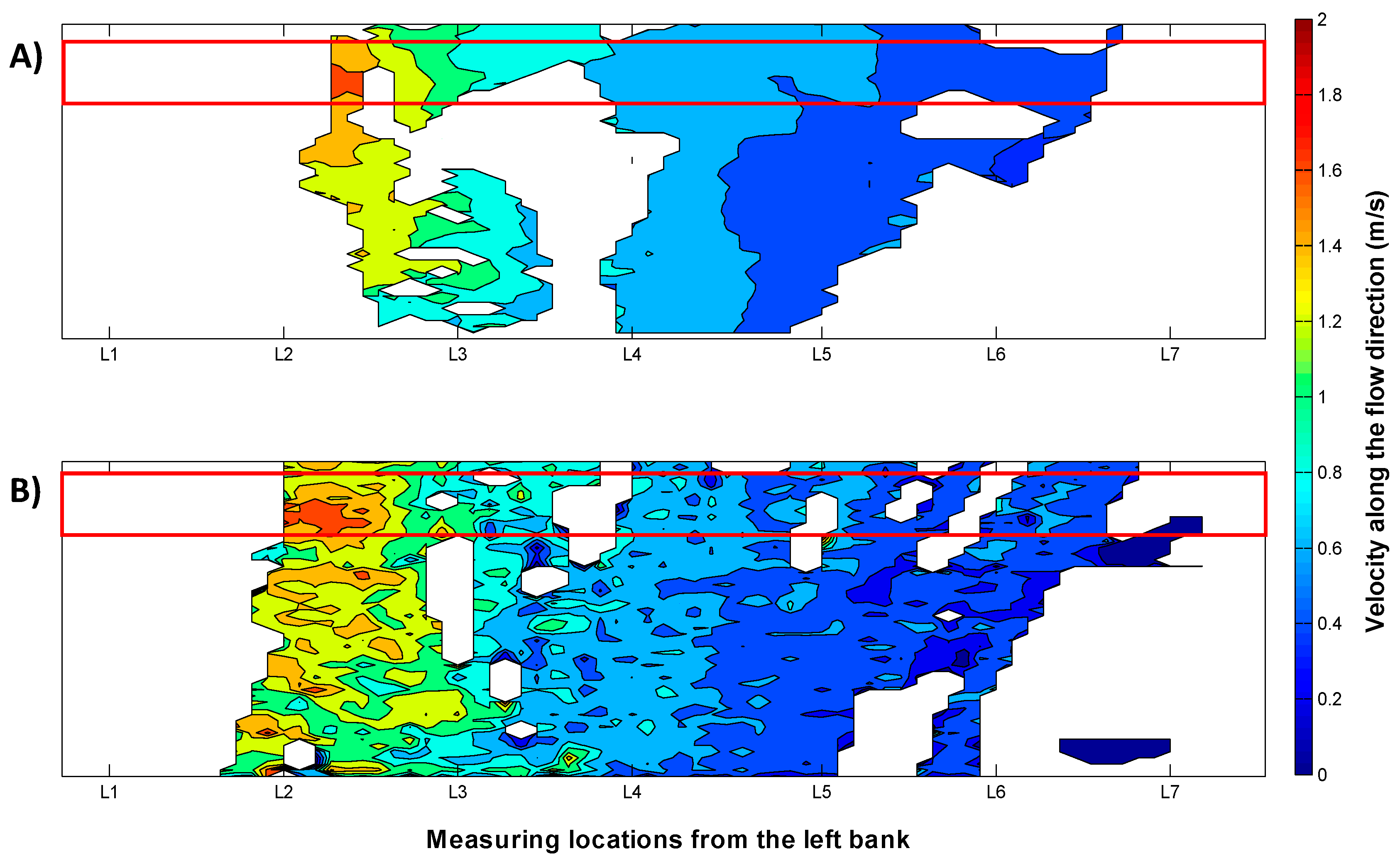
The Noce River campaign was characterised by medium seeding conditions (5.28 × 10⁻⁴ ppp), an average index of dispersion (9.09 ppp), and tracers with a relatively uniform dimension (CV_Area = 0.87). It was also characterised by significant light reflections on the free water surface. The effective seeding used in PTV analysis was reduced by 56% compared with the original detected seeding. Despite this, the presence of seeding along the cross-section allowed us to obtain satisfactory results using the PTV algorithm (RMSE = 0.049 m/s). LSPIV seemed to be more affected by the influence of the noise of environmental conditions. This was manifested as more unstable results along the cross-section, probably because velocity vectors were obtained by averaging the displacement of many features transiting in the interrogation windows, increasing the chances of catching noisy features in the analysis.

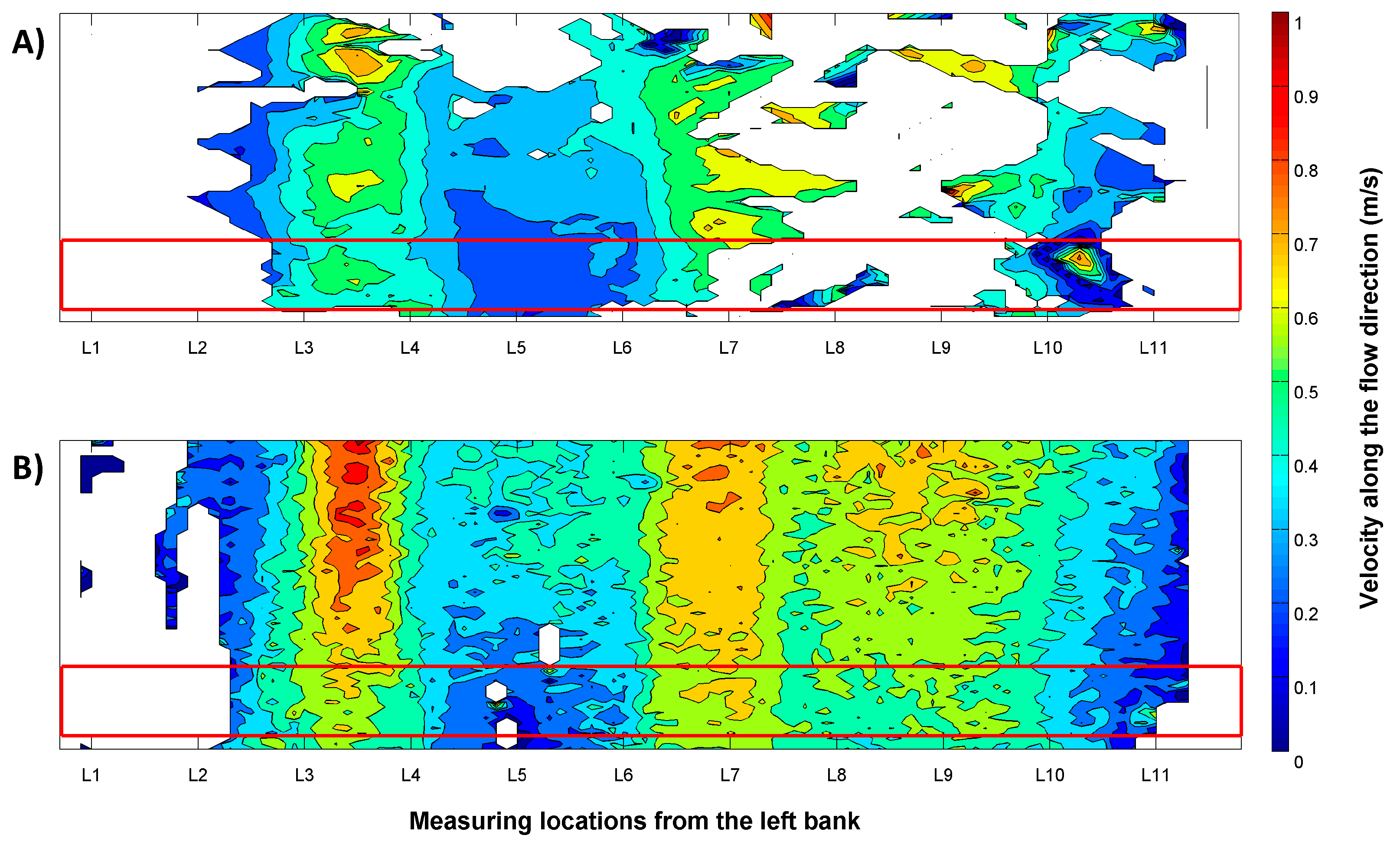
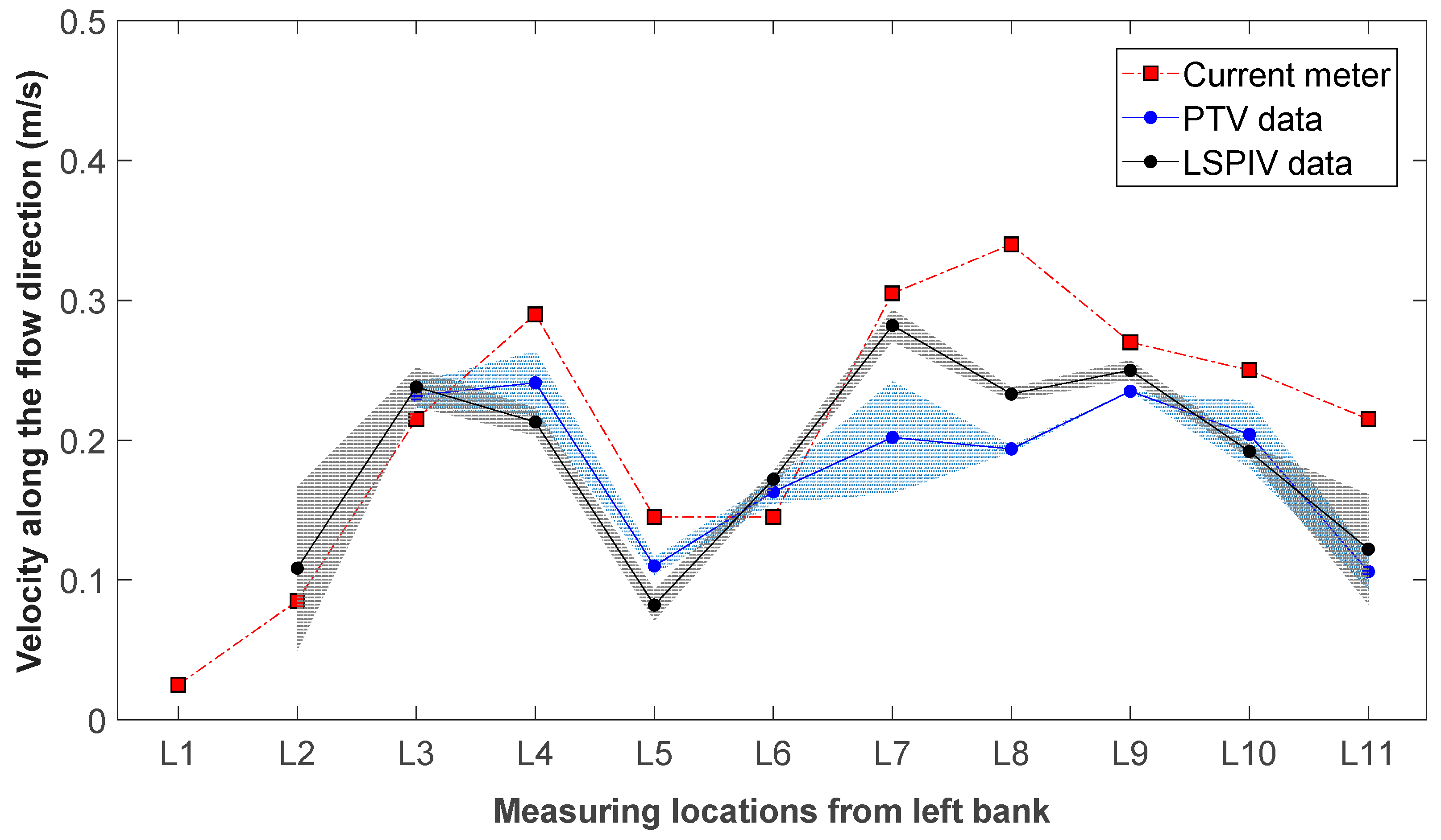
The Bradano River was characterised by very low seeding density (4.99 × 10⁻⁵ ppp), and a lower dispersion index (1.72 ppp) and coefficient of variation of tracer area (CV_Area = 0.35). Environmental conditions and more homogeneous seeding characteristics favoured an effective seeding reduction of only 19% with respect to the original estimated seeding. Low seeding affected the calculation of velocity over locations from FW1 to FW4, especially for PTV, due to the lack of tracking features. LSPIV with the FFT correlation approach allowed us to obtain reliable estimations for high and low velocities. Both techniques produced reliable results in close agreement with reference velocity measurements.

The Basento River was characterised by higher seeding conditions compared with the others (1.40 × 10⁻³ ppp). Tracers presented irregular shapes and dimensions (CV_Area = 1.76), with high dispersion in the field of view (20.37 ppp). The effect of the non-uniform characteristics of tracers and environmental conditions negatively impacted the results of both techniques, stressing the matching and tracking process. The effective seeding used by PTV was reduced by 81%, with an average value of 7.3 × 10⁻⁵ (ppp), leading to only a few meaningful trajectories. This produced a significant underestimation of surface velocities.

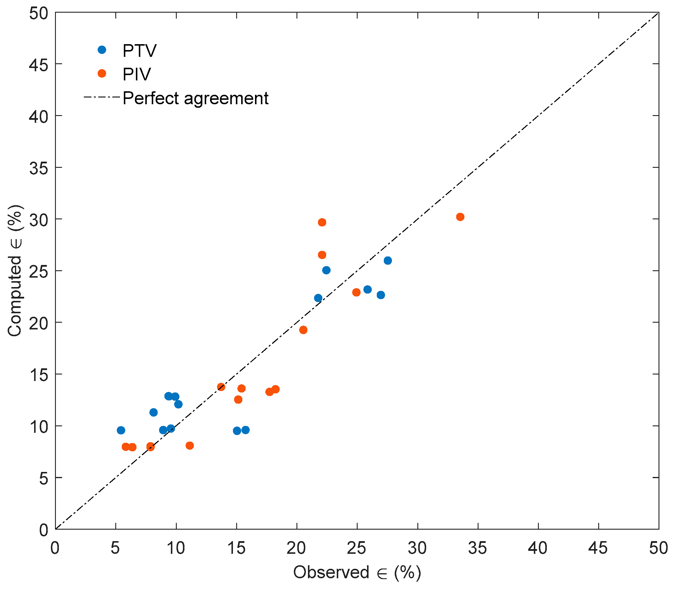
These three metrics were investigated through multiple linear regression analysis to evaluate the influence of seeding characteristics on surface velocity estimation. For both techniques, the results demonstrated that seeding density, the coefficient of variation of tracer dimension, and dispersion index have a similar influence on the accuracy of image velocimetry. In particular, statistical analysis corroborated the importance of seeding density for minimising estimation errors and showed that increasing the coefficient of variation of the tracer dimension and the dispersion index can negatively impact the final results. This suggests that the duration of video recording during field surveys should be increased, allowing the selection of optimal frame windows for analysis to minimise computed velocimetry errors. Increasing the number of frames allows covering different portions of the ROI by features, consequently allowing the computation of velocities across the whole ROI. This is especially important for riverbanks that are often difficult to seed (e.g., Bradano River). Previous experimental findings (e.g., [8,20]) support using an increased number of frames to improve the final results with lower variability of velocity estimations.

5. Conclusions

In this study, we focused on the accuracy of PTV and LSPIV image velocimetry techniques under different seeding conditions for three case study locations in Southern Italy. Our findings showed that PTV and LSPIV are sensitive to seeding and tracer characteristics as well as challenging environmental conditions. The seeding density that is effectively used by PTV in the analysis can be reduced up to 81% of the original, highlighting its applicability at very low seeded flows. This leads to an underestimation of flow velocity and, consequently, river discharge. For both techniques, the statistical analysis demonstrated that three metrics (seeding density, dispersion index, and spatial variance of tracer dimension) have a statistically significant influence on the accuracy of velocity estimation and can be used for a priori evaluation of flow seeding conditions. Increasing the number of frames can help with conducting complete velocity field characterisation because it increases the chance of having transiting features on the whole ROI. Consequently, more extended video registration and preliminary quantification of seeding characteristics can help with selecting an appropriate interval to process, image velocimetry technique to apply and related setting parameters, and in controlling the accuracy of results. Future studies should focus on implementing an automatic workflow to enhance the frames in particularly challenging conditions, such as intense sunlight, shadows, and ripples, to better emphasise and discriminate floater objects with respect to the background. Finally, we are currently working with a larger dataset to generalize the multiple regression equation for prediction purposes.

References

1. Fujita, I.; Muste, M.; Kruger, A. Large-scale particle image velocimetry for flow analysis in hydraulic engineering applications. J. Hydraul. Res. 1998, 36, 397–414. [Google Scholar] [CrossRef]
2. Kantoush, S.A.; Schleiss, A.J.; Sumi, T.; Murasaki, M. LSPIV implementation for environmental flow in various laboratory and field cases. J. Hydro-Environ. Res. 2011, 5, 263–276. [Google Scholar] [CrossRef] [Green Version]
3. Tauro, F.; Selker, J.; Van De Giesen, N.; Abrate, T.; Uijlenhoet, R.; Porfiri, M.; Manfreda, S.; Caylor, K.; Moramarco, T.; Benveniste, J.; et al. Measurements and observations in the XXI century (MOXXI): Innovation and multi-disciplinarity to sense the hydrological cycle. Hydrol. Sci. J. 2018, 63, 169–196. [Google Scholar] [CrossRef] [Green Version]
4. Bandini, F.; Lüthi, B.; Peña-Haro, S.; Bauer-Gottwein, P. A Drone-Borne Contactless Method to Jointly Estimate Discharge and Manning’s Roughness in Rivers. In EGU General Assembly 2020; EGU2020-4229 2020; Available online: https://meetingorganizer.copernicus.org/EGU2020/EGU2020-4229.html (accessed on 4 May 2020).
5. Tauro, F.; Piscopia, R.; Grimaldi, S. Streamflow Observations From Cameras: Large-Scale Particle Image Velocimetry or Particle Tracking Velocimetry? Water Resour. Res. 2017, 53, 10374–10394. [Google Scholar] [CrossRef] [Green Version]
6. Pearce, S.; Ljubičić, R.; Peña-Haro, S.; Perks, M.; Tauro, F.; Pizarro, A.; Dal Sasso, S.; Strelnikova, D.; Grimaldi, S.; Maddock, I.; et al. An Evaluation of Image Velocimetry Techniques under Low Flow Conditions and High Seeding Densities Using Unmanned Aerial Systems. Remote Sens. 2020, 12, 232. [Google Scholar] [CrossRef] [Green Version]
7. Perks, M.; Sasso, S.F.D.; Hauet, A.; Coz, J.L.; Pearce, S.; Peña-Haro, S.; Tauro, F.; Grimaldi, S.; Hortobágyi, B.; Jodeau, M.; et al. Towards harmonization of image velocimetry techniques for river surface velocity observations. Earth Syst. Sci. Data Discuss. 2019. in review. [Google Scholar] [CrossRef] [Green Version]
8. Manfreda, S.; Sasso, S.F.D.; Pizarro, A.; Tauro, F. New Insights Offered by UAS for River Monitoring. In Applications of Small Unmanned Aircraft Systems; Sharma, J.B., Ed.; CRC Press: Boca Raton, FL, USA, 2019; Volume 211. [Google Scholar]
9. Manfreda, S.; McCabe, M.F.; Miller, P.E.; Lucas, R.; Madrigal, V.P.; Mallinis, G.; Dor, E.B.; Helman, D.; Estes, L.; Ciraolo, G.; et al. On the use of unmanned aerial systems for environmental monitoring. Remote Sens. 2018, 10, 641. [Google Scholar] [CrossRef] [Green Version]
10. Le Boursicaud, R.; Pénard, L.; Hauet, A.; Thollet, F.; Le Coz, J. Gauging extreme floods on YouTube: Application of LSPIV to home movies for the post-event determination of stream discharges. Hydrol. Process. 2016, 30, 90–105. [Google Scholar] [CrossRef] [Green Version]
11. Le Coz, J.; Hauet, A.; Pierrefeu, G.; Dramais, G.; Camenen, B. Performance of image-based velocimetry (LSPIV) applied to flash-flood discharge measurements in Mediterranean rivers. J. Hydrol. 2010, 394, 42–52. [Google Scholar] [CrossRef] [Green Version]
12. Tauro, F.; Tosi, F.; Mattoccia, S.; Toth, E.; Piscopia, R.; Grimaldi, S. Optical Tracking Velocimetry (OTV): Leveraging Optical Flow and Trajectory-Based Filtering for Surface Streamflow Observations. Remote Sens. 2018, 10, 2010. [Google Scholar] [CrossRef] [Green Version]
13. Perks, M.T.; Russell, A.J.; Large, A.R.G. Technical note: Advances in flash flood monitoring using unmanned aerial vehicles (UAVs). Hydrol. Earth Syst. Sci. 2016, 20, 4005–4015. [Google Scholar] [CrossRef] [Green Version]
14. Strelnikova, D.; Paulus, G.; Käfer, S.; Anders, K.-H.; Mayr, P.; Mader, H.; Scherling, U.; Schneeberger, R. Drone-Based Optical Measurements of Heterogeneous Surface Velocity Fields around Fish Passages at Hydropower Dams. Remote Sens. 2020, 12, 384. [Google Scholar] [CrossRef] [Green Version]
15. Kim, Y.; Muste, M.; Hauet, A.; Krajewski, W.F.; Kruger, A.; Bradley, A. Stream discharge using mobile large-scale particle image velocimetry: A proof of concept. Water Resour. Res. 2008, 44, 261. [Google Scholar] [CrossRef]
16. Eltner, A.; Sardemann, H.; Grundmann, J. Technical Note: Flow velocity and discharge measurement in rivers using terrestrial and unmanned-aerial-vehicle imagery. Hydrol. Earth Syst. Sci. 2020, 24, 1429–1445. [Google Scholar] [CrossRef] [Green Version]
17. Tauro, F.; Petroselli, A.; Arcangeletti, E. Assessment of drone-based surface flow observations. Hydrol. Process. 2016, 30, 1114–1130. [Google Scholar] [CrossRef]
18. Le Coz, J.; Jodeau, M.; Hauet, A.; Marchand, B.; Le Boursicaud, R. Image-Based Velocity and Discharge Measurements in Field and Laboratory River Engineering Studies Using the Free Fudaa-LSPIV Software. In Proceedings of the International Conference on Fluvial Hydraulics, RIVER FLOW, Lausanne, Switzerland, 3–5 September 2014; pp. 1961–1967. [Google Scholar]
19. Lewis, Q.W.; Lindroth, E.M.; Rhoads, B.L. Integrating unmanned aerial systems and LSPIV for rapid, cost-effective stream gauging. J. Hydrol. 2018, 560, 230–246. [Google Scholar] [CrossRef]
20. Dal Sasso, S.F.; Pizarro, A.; Samela, C.; Mita, L.; Manfreda, S. Exploring the optimal experimental setup for surface flow velocity measurements using PTV. Environ. Monit. Assess. 2018, 190, 460. [Google Scholar] [CrossRef]
21. Tauro, F.; Petroselli, A.; Porfiri, M.; Giandomenico, L.; Bernardi, G.; Mele, F.; Spina, D.; Grimaldi, S. A novel permanent gauge-cam station for surface-flow observations on the Tiber River. Geosci. Instrum. Methods Data Syst. 2016, 5, 241–251. [Google Scholar] [CrossRef] [Green Version]
22. Leitão, J.P.; Peña-Haro, S.; Lüthi, B.; Scheidegger, A.; Moy de Vitry, M. Urban overland runoff velocity measurement with consumer-grade surveillance cameras and surface structure image velocimetry. J. Hydrol. 2018, 565, 791–804. [Google Scholar] [CrossRef]
23. Detert, M.; Weitbrecht, V. A low-cost airborne velocimetry system: Proof of concept. J. Hydraul. Res. 2015, 53, 532–539. [Google Scholar] [CrossRef]
24. Tauro, F.; Grimaldi, S. Ice dices for monitoring stream surface velocity. J. Hydro-Environ. Res. 2017, 14, 143–149. [Google Scholar] [CrossRef]
25. Huang, H.; Dabiri, D.; Gharib, M. On errors of digital particle image velocimetry. Meas. Sci. Technol. 1997, 8, 1427. [Google Scholar] [CrossRef]
26. Keane, R.D.; Adrian, R.J. Theory of cross-correlation analysis of PIV images. Appl. Sci. Res. 1992, 49, 191–215. [Google Scholar] [CrossRef]
27. Muste, M.; Fujita, I.; Hauet, A. Large-scale particle image velocimetry for measurements in riverine environments. Water Resour. Res. 2008, 44, 1–14. [Google Scholar] [CrossRef] [Green Version]
28. Pizer, S.M.; Amburn, E.P.; Austin, J.D.; Cromartie, R.; Geselowitz, A.; Greer, T.; ter Haar Romeny, B.; Zimmerman, J.B.; Zuiderveld, K. Adaptive histogram equalization and its variations. Comput. Vis. Graph. Image Process. 1987, 39, 355–368. [Google Scholar] [CrossRef]
29. Gonzalez, R.C.; Wintz, P. Digital Image Processing, 2nd ed.; Addison-Wesley: Boston, MA, USA, 1987. [Google Scholar]
30. Shavit, U.; Lowe, R.J.; Steinbuck, J.V. Intensity Capping: A simple method to improve cross-correlation PIV results. Exp. Fluids 2007, 42, 225–240. [Google Scholar] [CrossRef]
31. Tauro, F.; Grimaldi, S.; Petroselli, A.; Porfiri, M. Fluorescent particle tracers for surface flow measurements: A proof of concept in a natural stream. Water Resour. Res. 2012, 16, 2973–2983. [Google Scholar] [CrossRef] [Green Version]
32. Lin, D.; Grundmann, J.; Eltner, A. Evaluating Image Tracking Approaches for Surface Velocimetry with Thermal Tracers. Water Resour. Res. 2019, 55, 3122–3136. [Google Scholar] [CrossRef]
33. Kinzel, P.J.; Legleiter, C.J. sUAS-Based Remote Sensing of River Discharge Using Thermal Particle Image Velocimetry and Bathymetric Lidar. Remote Sens. 2019, 11, 2317. [Google Scholar] [CrossRef] [Green Version]
34. Brevis, W.; Niño, Y.; Jirka, G.H. Integrating cross-correlation and relaxation algorithms for particle tracking velocimetry. Exp. Fluids 2011, 50, 135–147. [Google Scholar] [CrossRef]
35. Tauro, F.; Piscopia, R.; Grimaldi, S. PTV-Stream: A simplified particle tracking velocimetry framework for stream surface flow monitoring. Catena 2019, 172, 378–386. [Google Scholar] [CrossRef]
36. Raffel, M.; Willert, C.E.; Scarano, F.; Kähler, C.J.; Wereley, S.T.; Kompenhans, J. Particle Image Velocimetry: A Practical Guide; Springer: Berlin/Heidelberg, Germany, 2018; ISBN 3319688529. [Google Scholar]
37. Kähler, C.J.; Scholz, U.; Ortmanns, J. Wall-shear-stress and near-wall turbulence measurements up to single pixel resolution by means of long-distance micro-PIV. Exp. Fluids 2006, 41, 327–341. [Google Scholar]
38. Pizarro, A.; Dal Sasso, S.F.; Perks, M.T.; Manfreda, S. Spatial distribution of tracers for optical sensing of stream surface flow. Hydrol. Earth Syst. Sci. Discuss. Rev. 2020. in review. [Google Scholar] [CrossRef]
39. Carter, R.W.; Anderson, I.E. Accuracy of current meter measurements. J. Hydraul. Div. Proc. ASCE 1963, 4, 105–115. [Google Scholar]
40. International Standards Organization (ISO). Measurement of Liquid Flow in Open Channel—Velocity-Area Method; ISO 748; ISO: Geneva, Switzerland, 1997. [Google Scholar]
41. Rosten, E.; Porter, R.; Drummond, T. Faster and better: A machine learning approach to corner detection. IEEE Trans. Pattern Anal. Mach. Intell. 2008, 32, 105–119. [Google Scholar] [CrossRef] [PubMed] [Green Version]
42. Fischler, M.A.; Bolles, R.C. Random sample consensus: A paradigm for model fitting with applications to image analysis and automated cartography. Commun. ACM 1981, 24, 381–395. [Google Scholar] [CrossRef]
43. Thielicke, W.; Stamhuis, E.J. PIVlab—Towards User-friendly, Affordable and Accurate Digital Particle Image Velocimetry in MATLAB. J. Open Res. Softw. 2014. [Google Scholar] [CrossRef] [Green Version]
Figure 1. Location of monitoring sites.
Remotesensing 12 01789 g001
Figure 2. Workflow of surface flow estimation, including seeding quantification and optical methods: (A) video acquisition; (B) image enhancement; (C) feature detection; (D) 2D flow velocity field.
Remotesensing 12 01789 g002
Figure 3. Frames acquired at (A) Noce, (B) Bradano, and (C) Basento Rivers. Dark zones represent frames after contrast stretching, enhancing the contrast between tracers and background. Regions of interest (ROIs) are shown in red squares and locations of reference velocity measurements as white crosses. The main flow direction is indicated by arrows. A zoom-in of the metric pole is shown in (C).
Remotesensing 12 01789 g003
Figure 4. Identification of features on (A) Noce, (B) Bradano and (C) Basento Rivers. Examples of detected features inside ROIs (red squares) are zoomed in (A′, B′, and C′).
Remotesensing 12 01789 g004
Figure 5. Comprehensive overview of seeding behaviour during considered acquisition time for each study case. (A) Seeding density in particles per pixel (ppp), (B) mean area of tracers in cm2, (C) dimensionless dispersion index, and (D) coefficient of variation of the tracers’ area.
Remotesensing 12 01789 g005
Figure 6. Examples of flow velocity maps calculated with (A) PTV and (B) LSPIV techniques for frame window FW4 on the Noce River. Red squares represent the ROI considered for the analysis.
Remotesensing 12 01789 g006
Figure 7. Comparison between surface velocity estimation computed with PTV (blue line) and LSPIV (black line) for experiments carried out in the Noce River at different frame windows. Shaded regions indicate standard deviations between frame sequences. Values recorded with the current meter are indicated by red squares.
Remotesensing 12 01789 g007
Figure 8. Examples of flow velocity maps calculated with (A) PTV and (B) LSPIV techniques for frame window FW5 on Bradano River. Red squares represent ROI considered for the analysis.
Remotesensing 12 01789 g008
Figure 9. Comparison between surface velocity estimations computed with PTV and LSPIV for experiments conducted in the Bradano River. Shaded regions indicate standard deviations between frame sequences. Values recorded with the current meter are indicated by red squares.
Remotesensing 12 01789 g009
Figure 10. Examples of flow velocity maps calculated using (A) PTV and (B) LSPIV algorithms on FW3 of the Basento River. Red squares represent ROI considered for the analysis.
Remotesensing 12 01789 g010
Figure 11. Comparison between surface velocity estimations computed with PTV and LSPIV for experiments conducted on frame windows in the Basento River. Shaded regions indicate standard deviations between frame sequences. Values recorded with the current meter are also reported.
Remotesensing 12 01789 g011
Figure 12. Error predicted by multiple regression analysis vs. error observed with PTV and LSPIV.
Remotesensing 12 01789 g012