Article

Evaluating Prediction Models for Mapping Canopy Chlorophyll Content Across Biomes

1
Faculty of Geo-Information Science and Earth Observation (ITC), University of Twente, 217, 7500 AE Enschede, The Netherlands
2
Department of Geography and Environmental Studies, Wollo University, 1145 Dessie, Ethiopia
3
Department of Environmental Science, Macquarie University, NSW 2106, Australia
4
Department of Visitor Management and National Park Monitoring, Bavarian Forest National Park, 94481 Grafenau, Germany
5
Chair of Wildlife Ecology and Wildlife Management, University of Freiburg, Tennenbacher Straße 4, D-79106 Freiburg, Germany
6
European Space Agency - ESRIN, Via Galileo Galilei, Casella Postale 64, 00044 Frascati (R.M.), Italy
7
German Aerospace Center (DLR), The Remote Sensing Technology Institute (IMF), German Aerospace Center (DLR), Münchener Str. 20, 82234 Weßling, Germany
8
Wageningen Environmental Research, Wageningen University, and Research, 47, 6700 AA Wageningen, The Netherlands
*
Author to whom correspondence should be addressed.
Remote Sens. 2020, 12(11), 1788; https://doi.org/10.3390/rs12111788
Submission received: 1 May 2020 / Revised: 21 May 2020 / Accepted: 30 May 2020 / Published: 1 June 2020

Abstract

:
Accurate measurement of canopy chlorophyll content (CCC) is essential for the understanding of terrestrial ecosystem dynamics through monitoring and evaluating properties such as carbon and water flux, productivity, light use efficiency as well as nutritional and environmental stresses. Information on the amount and distribution of CCC helps to assess and report biodiversity indicators related to ecosystem processes and functional aspects. Therefore, measuring CCC continuously and globally from earth observation data is critical to monitor the status of the biosphere. However, generic and robust methods for regional and global mapping of CCC are not well defined. This study aimed at examining the spatiotemporal consistency and scalability of selected methods for CCC mapping across biomes. Four methods (i.e., radiative transfer models (RTMs) inversion using a look-up table (LUT), the biophysical processor approach integrated into the Sentinel application platform (SNAP toolbox), simple ratio vegetation index (SRVI), and partial least square regression (PLSR)) were evaluated. Similarities and differences among CCC products generated by applying the four methods on actual Sentinel-2 data in four biomes (temperate forest, tropical forest, wetland, and Arctic tundra) were examined by computing statistical measures and spatiotemporal consistency pairwise comparisons. Pairwise comparison of CCC predictions by the selected methods demonstrated strong agreement. The highest correlation (R2 = 0.93, RMSE = 0.4371 g/m2) was obtained between CCC predictions of PROSAIL inversion by LUT and SNAP toolbox approach in a wetland when a single Sentinel-2 image was used. However, when time-series data were used, it was PROSAIL inversion against SRVI (R2 = 0.88, RMSE = 0.19) that showed greatest similarity to the single date predictions (R2 = 0.83, RMSE = 0.17 g/m2) in this biome. Generally, the CCC products obtained using the SNAP toolbox approach resulted in a systematic over/under-estimation of CCC. RTMs inversion by LUT (INFORM and PROSAIL) resulted in a non-biased, spatiotemporally consistent prediction of CCC with a range closer to expectations. Therefore, the RTM inversion using LUT approaches particularly, INFORM for ‘forest’ and PROSAIL for ‘short vegetation’ ecosystems, are recommended for CCC mapping from Sentinel-2 data for worldwide mapping of CCC. Additional validation of the two RTMs with field data of CCC across biomes is required in the future.

1. Introduction

Canopy chlorophyll content (CCC), the sum of chlorophyll a and b in a group of foliage per unit ground area, is a biodiversity variable highly related to ecosystem functioning and helps to understand the dynamics of photosynthesis, plant responses to environmental change, variation in genetics, and diversity in ecology [1]. CCC is an important indicator of ecosystem health and vegetation physiological status [2]. It is an essential variable in monitoring the terrestrial carbon budget by supporting an accurate estimate of primary productivities [3,4] used as an input parameter for biosphere models to predict carbon and water changes [5], and light use efficiency [6]. Information on the amount and distribution of CCC has been utilized to answer many ecological questions related to monitoring and evaluating terrestrial ecosystem properties such as identifying types of vegetation, mapping vegetation cover, and understanding the condition of vegetation [7]. Changes in CCC indicate the effects of disease, nutritional, and environmental stresses [8,9,10,11]. CCC can also be used for forage quality assessment, ecosystem classification, and biomass estimation, as well as being a key input to estimate the indicators for the Convention on Biological Diversity (CBD) such as trends in carbon stocks and patterns in resilience within ecosystems of Aichi target 15, and net primary productivity of Achi target 3 [12]. The spatially and temporally contiguous information on CCC can also be used to support measuring indicators of the sustainable development goals (SDGs) related to the sustainable use of terrestrial ecosystems.
Remote sensing provides the opportunity to drive comprehensive variables for assessing and monitoring biodiversity globally [13] and helps to fill the spatial and temporal gaps left by in situ observations. Thus, remote sensing data provide a viable solution to predict CCC and minimizes the effort by ecologists to collect chlorophyll data through laborious field surveys, cover relatively small extents and short temporal periods to track biodiversity changes.
There is a sturdy correlation between canopy reflectance and chlorophyll that could be used to estimate CCC from imagery. Recent advances in satellite sensors deliver increased resolution and sensitivity of spectral reflectance to CCC. Likewise, a multitude of vigorous methods has been established that correlate CCC and earth observation data [14,15,16,17,18]. The reflectance spectrum between 680 and 760 nm acquired using remote sensing sensors, which is referred to as the red edge position (REP), has been broadly utilized to predict leaf and canopy chlorophyll content [19,20]. This is because a surge in chlorophyll content leads to a shift in the absorption feature towards longer wavelengths [21]. In the literature, the approaches used to predict CCC from earth observation data are categorized into two broad classes: (1) empirical-based; and (2) physical-based [22,23]. Verrelst, et al. [24] further extended the algorithm classes into subclasses and combinations thereof: (i) parametric regression, (ii) non-parametric, (iii) physically-based, and (iv) hybrid methods. Each group of algorithms has its advantages and drawbacks, which are discussed in Verrelst, Camps-Valls [24].
Irrespective of the methods, the prediction accuracy of remotely sensed CCC is affected by factors such as soil type, the existence of non-green components, canopy structure, and shadows [25,26]. Moreover, differences in leaf internal structure, thickness, water content, leaf area index (LAI), foliage clumping, canopy closure, and background in different biomes may alter the relationship between CCC and reflectance [27,28]. Heterogeneity of land surface texture is another source of error when locally developed algorithms up-scaled to regional and global scales [29]. The absence of good-quality high-resolution imagery covering the entire Earth from one sensor may be solved by combining data obtained from multiple sensors, which increases the challenges of global mapping [30]. It is likely that leaves with the same reflectance spectra may have different reflectance factors in different forest canopies [31,32]. As a result transferring predictive models developed for one biome, universally across all biomes in broad spatial extents containing different species or plant functional types is challenging. Previous studies showed that CCC could be retrieved from hyperspectral remote sensing with high accuracy at a relatively small scale, but as soon as the observation level changes to landscape, the accuracy tends to weaken [33]. Algorithms initially developed at a local level are particularly affected by such additional heterogeneity dynamics if extrapolated over a larger extent [25,33,34].
Hence, CCC mapping across biomes for biodiversity monitoring in terrestrial ecosystems requires a reliable operational mapping strategy to be developed. A diversity of mapping schemes and classification methods were proposed for the global mapping of biophysical variables such as LAI and land cover products [35,36]. So far, the only available remote sensing-based chlorophyll products are from ENVISAT MERIS satellite data at 300 m spatial resolution including the MERIS terrestrial chlorophyll index (MTCI) [37], which is later modified to Sentinel-3 Ocean land color imager Terrestrial Chlorophyll Index (OTCI) [38], and the recently developed global distribution of leaf chlorophyll content with canopy and leaf-level radiative transfer modeling procedures [39]. To our knowledge, there are no algorithms validated across biomes for global mapping of CCC from high-resolution satellite imagery. Ali, et al. [40] has recently identified four potential methods that can be used for wide extent retrieval of CCC through a review of the-state-of-art algorithms and validated using in situ data namely simple ratio vegetation index (SRVI) and partial least square regression (PLSR) from statistical-based algorithms, and two physical-based algorithms: INFORM/PROSAIL inversion using a look-up table and the biophysical retrieval tool integrated into the Sentinel application platform (SNAP toolbox), which is a PROSAIL inversion using artificial neural network (ANN) (hereafter referred to as SNAP toolbox approach). To identifying the operationally feasible algorithm(s) that can be upscaled to regional and global levels demands evaluating their accuracy, temporal stability, and transferability across different biomes. Therefore, this study evaluated the robustness and spatiotemporal consistency of those methods proposed by Ali, Darvishzadeh [40] for large scale mapping of CCC for biodiversity monitoring in terrestrial ecosystems. Specifically, we aimed at pairwise comparison of the four methods performance in different pilot sites of major biomes in retrieving CCC from freely available satellite observations, focusing on Sentinel-2.

2. Materials and Methods

2.1. Pilot Sites

To verify and validate the adequacy of the proposed algorithm(s) for monitoring CCC at a large scale, the selected pilot sites should represent the major biomes of terrestrial ecosystems. Four Biomes (i.e., (1) Boreal Taiga and Artic Tundra, (2) Wetlands, (3) Temperate/Mediterranean forests, and (4) Tropical/sub-tropical rain forest) with diverse vegetation types across gradients of climate, altitude, and latitude were considered. Each biome is represented by one pilot site (Figure 1). The selected four pilot sites from four terrestrial biomes were:
  • Kytalyk (Arctic tundra) is located south of the East Siberian Sea coast, Russia (79.82°N, 147.47°E). It is part of a low-Arctic tundra nature reserve in the Indigirka lowlands. The site is characterized by very thick (>100-meter depth) ice-rich permafrost [41]. Kytalyk is a habitat of different tundra vegetation types, including tussock sedge, short shrubs, and moss tundra [42].
  • La Camargue (wetland ecosystem) is one of the Ramsar sites, which is a biosphere reserve in the Rhône delta in Southern France (43.53°N, 4.50°E). The major natural habitats of La Camargue contain lagoons, brackish/freshwater marshes, halophilous scrubs, and steppes. In this ecosystem, rice and irrigated crops are predominantly intermingled with the natural wetland vegetation. Camargue is a species-rich Mediterranean wetland with more than 1200 plant species [43]. The quality and quantity of water that is available year-round highly influence the functional diversity of the pilot site. Significant parts of Camargue naturally dry up during the summer season [44].
  • Bavarian Forest National Park (temperate forest) is a temperate forest found in Southeastern Germany (48.96°N, 13.39°E) along the border between Germany and the Czech Republic. The soils of the BFNP (Bavarian Forest National Park) are predominantly acid and have poor nutrient content. Loose brown, brown, and podsol brown soils are the three main soil types in the pilot site. The park is characterized by high annual precipitation (1200–1800 mm) and low temperature 3.5–6.5 °C in the valleys, 4.4–7.2 °C on the hillsides, and 2.0–5.0 °C in the higher montane zones [45]. Norway spruce (Picea abies) and European beech (Fagus sylvatica) are the two dominant tree species in the area [46].
  • Lambir National Park (tropical/sub-tropical rainforests) is part of Lambir Hills National Park in Sarawak, an East Malaysian state in Borneo (4.21°N, 114.03°E). It is a lowland tropical forest with an altitude range between 150–465 meters asl. The park is mainly a dipterocarp forest mixed with some patches of heath forest [47].

2.2. Satellite Imagery

To assess and compare the robustness and spatiotemporal consistency of the chosen methods in predicting CCC from remote sensing data for global prediction, Sentinel-2 images of the pilot areas were utilized. Sentinel-2 Level 1C products acquired in 2017 and/or 2018 on a relatively cloud-free date(s) (< 10% cloud cover) in each pilot site were used. As indicated in Table 1, 24 Sentinel-2 images in total were downloaded from the ESA Copernicus open access hub (https://scihub.copernicus.eu) for this study.
Sentinel-2 has three sets of spatial resolution (i.e., 10 m, 20 m, and 60 m). Spectral reflectance in the visible and NIR and SWIR spectral regions are acquired in four, six, and three bands at each spatial resolution, respectively (Table 2). The Sen2cor vs. 2.5.5 stand-alone software, which is freely distributed under the GNU general public license (http://step.esa.int/main/third-party-plugins-2/sen2cor/), was used to perform atmospheric correction and produce surface reflectance (level 2A product) from the top-of-atmosphere (TOA) reflectance of Sentinel-2 (level 1c product). The level 2A product was resampled to 20 m spatial resolution, and spectral information in only ten bands (bands 2, 3, 4, 5, 6, 7, 8, 8a, 11, and 12) were used in this study.

2.3. Methods

2.3.1. Selected Algorithms

We investigated the robustness and spatiotemporal consistency of various approaches to understanding their potential, limitations, and transferability across biomes. More details about the following selected methods can be found in Ali, Darvishzadeh [40].
(a)
Simple ratio vegetation indices
Two simple ratio vegetation indices optimized for forests and non-forest vegetation were used. The SRVIs use spectral information in two spectral bands to compute CCC. During experimental analysis, Ali, Darvishzadeh [40] revealed that the simple ratio vegetation index 1 (SRVI_1) of Sentinel-2 band 8a (865 nm) and band 4 (665 nm) as a good predictor of CCC in a forest ecosystem (Equation (1)). Another simple ratio vegetation index (SRVI_2) of Inoue, Guérif [10], which is calibrated and validated for retrieving CCC from remote sensing data for a wide range of crops and natural grasses (Equation (2)) was used for non-forest vegetation.
SRVI - 1 = B 8 a B 4 = R 865 R 665
SRVI - 2 = B 8 B 5 = R 835 R 704
where R865, R835, R704, and R665 are reflectances in the center wavelengths of the Sentinel-2 band setting.
CCC was then generated by applying the fitting equations (Equations (3) and (4)) proposed for the two SRVIs on Sentinel-2 level 2A product (TOC reflectance).
CCC (g/m2) in forest = 0.071*SRVI-1 + 0.217
CCC (g/m2) in ‘short vegetation’ = 0.325 *SRVI-2 − 0.358
(b)
Partial least square regression (PLSR)
Among the non-parametric regression methods, the PLSR was utilized to generate CCC products at the four pilot sites. We used the PLSR trained on a spectral subset of eight bands (B2, B3, B4, B5, B6, B8a, B11, and B12) of Sentinel-2 with five components, which was found to be the accurate setup for CCC retrieval from Sentinel-2 data after testing different subsets of spectral information and optimizing the number of components of explanatory variables. The selected bands were those which showed higher variables importance in the projection (≥1) during the PLSR training.
(c)
INFORM and PROSAIL radiative transfer models inversion using look-up table (LUT)
The CCC products predicted by radiative transfer models (RTMs) inversion were performed by coupling the PROSPECT leaf model with two canopy models: Scattering by Arbitrarily Inclined Leaves (SAIL), and Invertible Forest Reflectance model (INFORM). The two RTMs were used to simulate and generate LUTs for non-forest and forest vegetation pilot sites’ Sentinel-2 spectra. Then merit functions applied on the LUTs to retrieve the CCC products. The essential elements of the parametrization, LUT generation, and inversion using the INFORM and PROSAIL models are described briefly below.
(i)
Parameterization and generation of LUT using INFORM
INFORM [27,48] is parameterized by leaf, canopy, and sensor parameters (Table 3) to generate the spectral reflectance of forests. A LUT is built by changing the inputs randomly within their range. It is always a trade-off between the size of the LUT and the computation time of the inversion. The larger the size of the LUT, the higher the chance of the simulated spectra contain all possible combinations of the input parameters, but the inversion becomes computationally expensive. Therefore, a LUT of 200,000 spectra was used, which was a recommendation of several authors [49,50]. To account for model uncertainties and reduce auto-correlation between the spectrum and input variables, a random Gaussian noise value of 0.3% was added to each simulated spectrum.
(ii)
Parameterization and generation of LUT using PROSAIL
PROSAIL is used for the generation of the canopy reflectance spectra of ‘short vegetation’ such as wetlands, taiga, and tundra. Spectral simulation using PROSAIL requires leaf, canopy, and sensor configuration parameters. A list of the parameters used and their range based on prior knowledge in the literature are presented in Table 4.
A LUT of 100,000 spectra were built by varying the inputs randomly within their range. This size of LUT has been confirmed to be large enough for retrieval of vegetation properties in different vegetation [50,51,52,53]. Similar to the INFORM spectra, a random Gaussian noise value of 0.3% was added to each simulated spectrum.
(iii)
LUTs Inversion
For both LUT generated by INFORM and PROSAIL, LUT inversion demands searching for each measured spectra (Sentinel-2) it is matching from the simulated spectra (INFORM or PROSAIL). The least root mean square error (RMSE) was the criterion to find the matching spectra through a comparison of the measured and simulated spectra (Equation (5)).
R M S E = ( R m e a s u r e d R s i m u l a t e d ) 2 n
where Rmeasured is a Sentinel-2 reflectance at wavelength λ, and Rsimulated is a spectrum at wavelength λ in the LUT, and n stands for the number of wavelengths.
The LUT based CCC retrieval was performed using three Sentinel-2 bands, which are located in the red, red-edge, and NIR transition zone. This region of the electromagnetic spectrum known for its sensitivity for subtle variation in chlorophyll. The group of input variables that provided the spectra in the LUT with the least RMSE was taken as the best estimates. However, simplification of reality in the RTM and parameterization, as well as calibration and atmospheric correction errors in the remote sensing dataset, the lowest RMSE criterion might not certainly offer the best solution. Consequently, for each Sentinel-2 (measured) spectrum, the 100 similar spectra with relatively smaller RMSE were obtained from the LUT. From the 100 available solutions (q), the median spectrum CCC value was taken as a final solution.
(d)
SNAP toolbox approach
Baret [56] proposed retrieval of vegetation biophysical variables by training the ANN on PROSAIL simulated spectra and inverting on atmospherically corrected (surface reflectance) data of Sentinel-2. This approach is grouped under the category of ‘hybrid’ model by Verrelst, Camps-Valls [24], and has been implemented in the Sentinel Application Platform (SNAP) toolbox. The method uses normalized Sentinel-2 data in eight bands (B3 – B7, B8a, B11, and B12), as well as sensor observation and illumination angles, and predicts vegetation biophysical variables such as LAI, fraction of absorbed photosynthetically active radiation, fraction of vegetation cover, CCC, and water content together with a quality flag product for each SNAP biophysical product. The CCC quality flag was used to mask out pixels with input and/or output out of range values. The unit of the CCC product in SNAP is µg/cm2; however, in our study, we applied a conversion factor to convert it to g/m2. See Baret [56] for details of the approach.

2.3.2. Assessment of Methods Transferability

The traditional validation of remote sensing methods requires the collection of in situ data concurrent with the acquisition of remote sensing data. Acquiring such in situ dataset from a range of biomes representing a logical subset of the whole terrestrial ecosystems is very expensive and time-consuming, and thus not feasible. To overcome this limitation and quantitatively compare the selected algorithms for regional and global scale CCC mapping, the following verification (validation) strategies were used.
(a)
Spatial distribution consistency
The spatial distribution of CCC maps produced using the approaches described in Section 2.3.1 was visually and quantitatively investigated for each pilot site in the four biomes. The ranges of the generated CCC products were compared to the expected CCC range in each biome.
A random sample up to 200 pixels was extracted from each CCC product and used in a paired t-test, (assuming the null hypothesis that pairs maps were identical to each other regardless of which algorithm was used) to examine whether the mean difference in CCC from one map to another was different than would be expected by chance alone. We also applied the two-sample Kolmogorov-Smirnov test [59], which is a non-parametric hypothesis test that evaluates the difference between two distributions, to measure disparities among pairs of CCC products.
(b)
A measure of agreement among pairwise CCC products
The closeness of the CCC predicted values by pairs of methods was evaluated by computing the strength of the correlation, prediction errors, and precision. The randomly extracted 200 samples of CCC values from each map were used to calculate the coefficient of determination (R2) (Equation (6)), root mean square error (RMSE) (Equation (7)), and Bias (Equation (8)). The more similar pairs of products are the ones with higher R2, lower RMSE, and bias close to zero.
R 2 = 1 ( y i y i ) 2 ( y i y i ¯ ) 2
R M S E = ( y i y i ) 2 n
B i a s = y i y i n
where y and y’ are the predicted values of the two methods for sample i, and n is the number of samples considered.
(c)
Temporal consistency
To examine the temporal consistency and robustness of the candidate algorithms, predictions of CCC were performed using time series Sentinel-2 data. It was evaluated whether the closeness of the predicted CCC values by a pair of methods significantly change through time. Therefore, the candidate algorithms were applied on cloud-free time-series Sentinel-2 data available for the period June 2017 to September 2018 for two of the pilot sites (BFNP and La Camargue) assuming the temporal consistency in these two sites represent the performance of the methods across tall (forest) and short (shrub and grassland) biomes. Sentinel-2 images acquired on the seven dates were used for BFNP. Whereas for La Camargue, fifteen dates of Sentinel-2 images were used. The statistical measures such as R2, RMSE, and bias (Equations (6)–(8)) were computed by using several dates of CCC values predicted by a pair of methods to assess how the relationship between pairs of algorithms change over time.

3. Results

3.1. Spatial Distribution Consistency

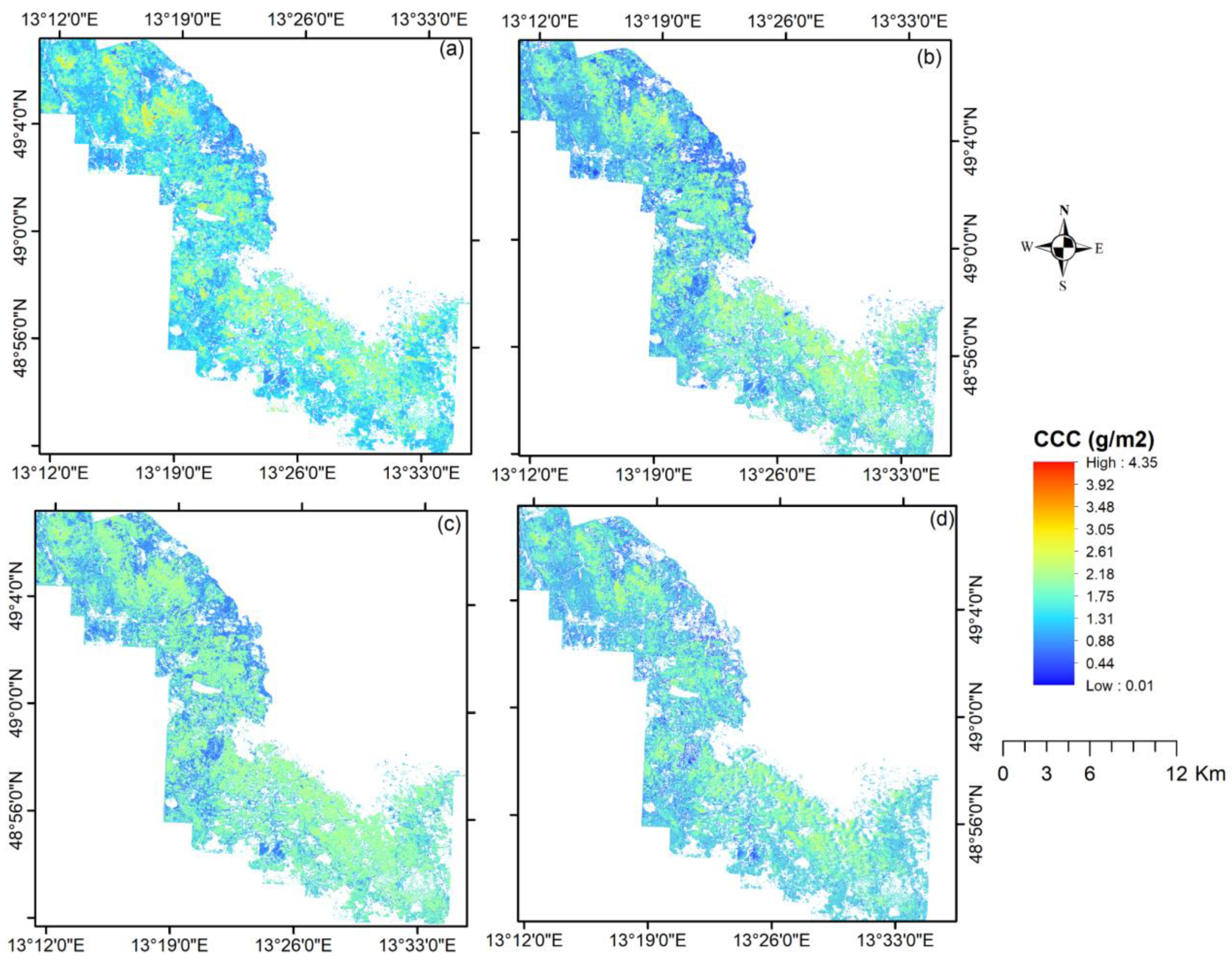
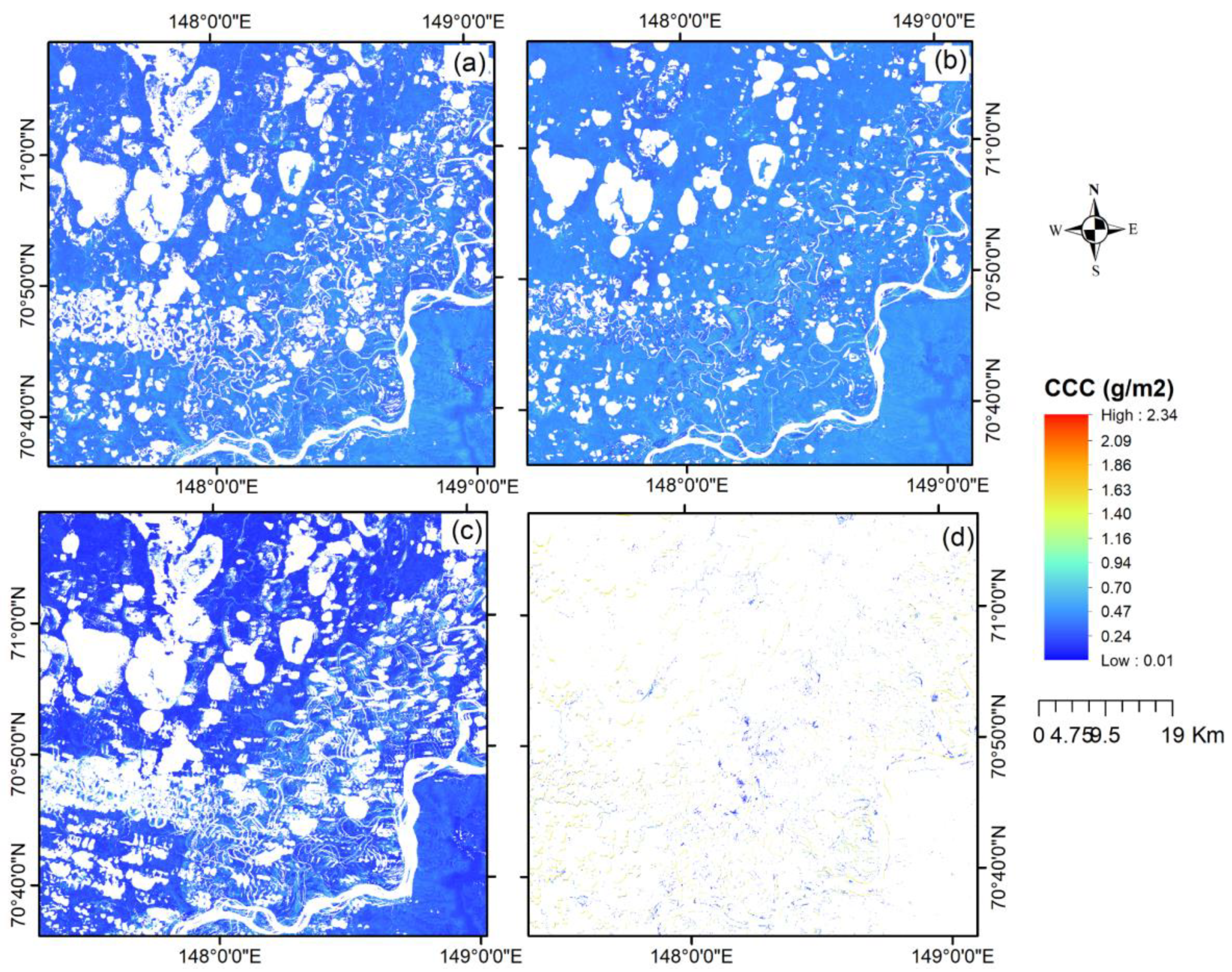
The expected and predicted CCC ranges are presented in Table 5. The INFORM and PROSAIL ranges are closer to expectations in three of the four biomes (temperate, wetland, and tundra). But, in tropical rain forests, it is the range obtained by the SNAP toolbox which is closest to expectations. Figure 2, Figure 3, Figure 4 and Figure 5 details the spatial distribution consistency of the CCC predictions by the candidate approaches in the four biomes.
Visually, the CCC maps generated by all methods showed a similar pattern in the BFNP (Figure 2). In this pilot site, generally, deciduous forests (mostly beech) showed higher CCC values. However, there are differences among the CCC products of the selected methods for the other three biomes. It is apparent from closer inspection of the four CCC maps generated for the tropical forest (Figure 3) that there is a more significant variation among the produced products compared to BFNP. The prediction made by the SNAP toolbox indicated higher CCC values in most parts of the Lambir pilot site (tropical forest) than other approaches. The CCC product from the PLSR method deviates from the other three approaches when applied in the Mediterranean wetland ecosystem (Figure 4) and tundra pilot sites (Figure 5), and thus no further statistical test performed for PLSR.
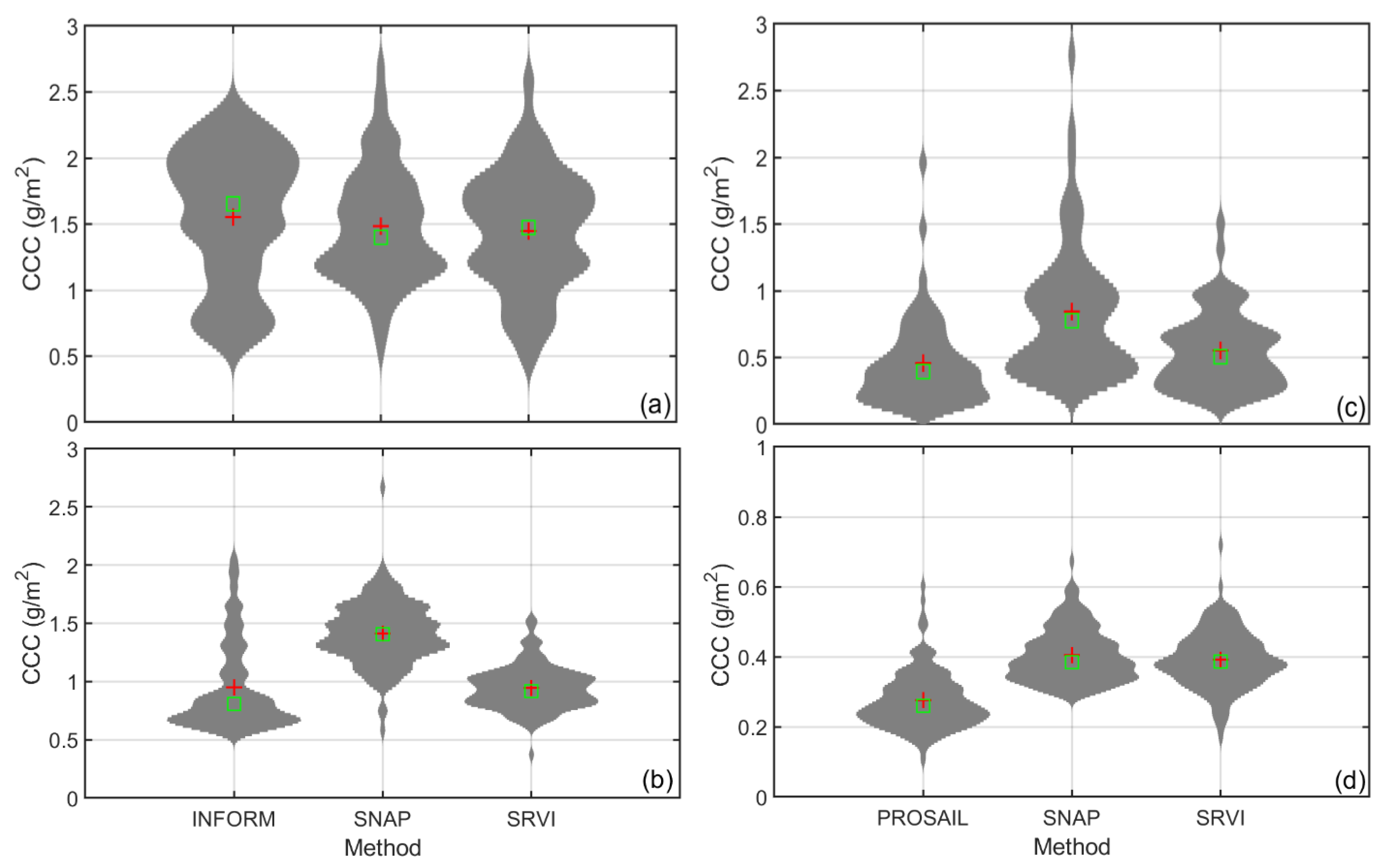
The two-sample Kolmogorov-Smirnov test among pairs of CCC products from INFORM, SRVI, and SNAP did not show significant distribution disparities in the temperate forest pilot site (Table 5). The Violin plot in Figure 6 depicts the similarities and differences of CCC products generated by the selected methods. In contrast, all of the pairs of CCC products showed distribution disparity in tropical rainforest, as shown in Table 6 and the violin plots in Figure 6c. Pairwise comparison of CCC predicted by PROSAIL and SRVI in La Camargue (wetland) exhibited similar distribution. In contrast, non-significant distribution disparity was observed between CCC products from the SNAP toolbox and SRVI in tundra biome (Table 5). However, the latter two methods predicted CCC values ranges in tundra biome were far beyond the expected range in Table 5.

3.2. The Agreement of CCC Values Predicted by the Selected Methods

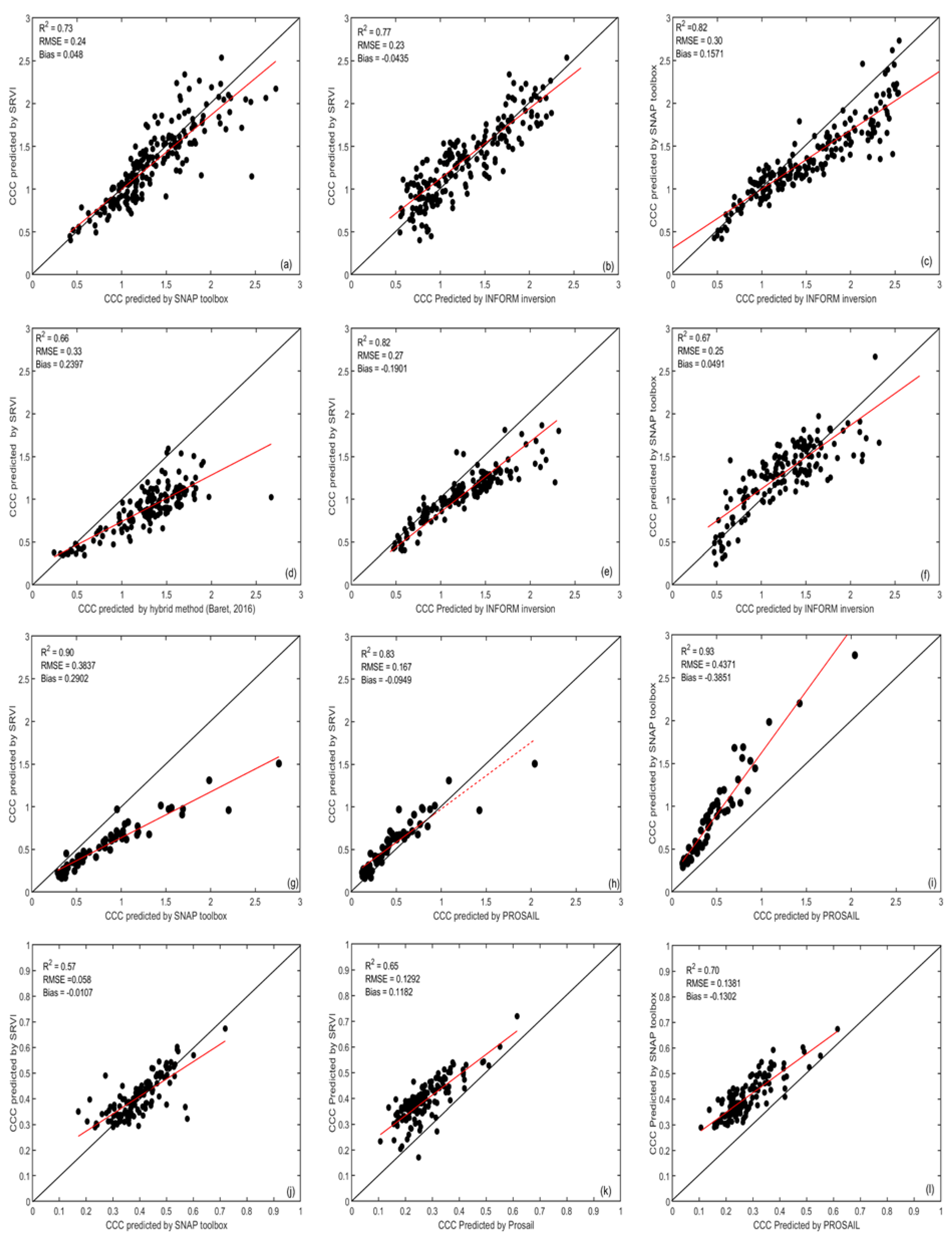
We verified how the CCC products generated by the methods chosen are close to each other across the four biomes. As illustrated in Figure 7, the CCC predicted by SRVI agrees with radiative transfer models (RTMs) inversion (INFORM inversion in forests or PROSAIL in short vegetation). The SRVI and RTMs inversion pairs had a higher correlation, lower RMSE, and the bias was close to zero in all the four pilot sites. However, the highest correlation (R2 = 0.93) was recorded for the SNAP toolbox approach with PROSAIL inversion (Figure 7i).
The predictions made using the SNAP toolbox approach [56] showed a tendency of overestimation, particularly in a wetland, when compared to SRVI and RTM inversion by LUT. There are weaker agreements between predictions in tundra than any other biome (Figure 7j).

3.3. Temporal Consistency

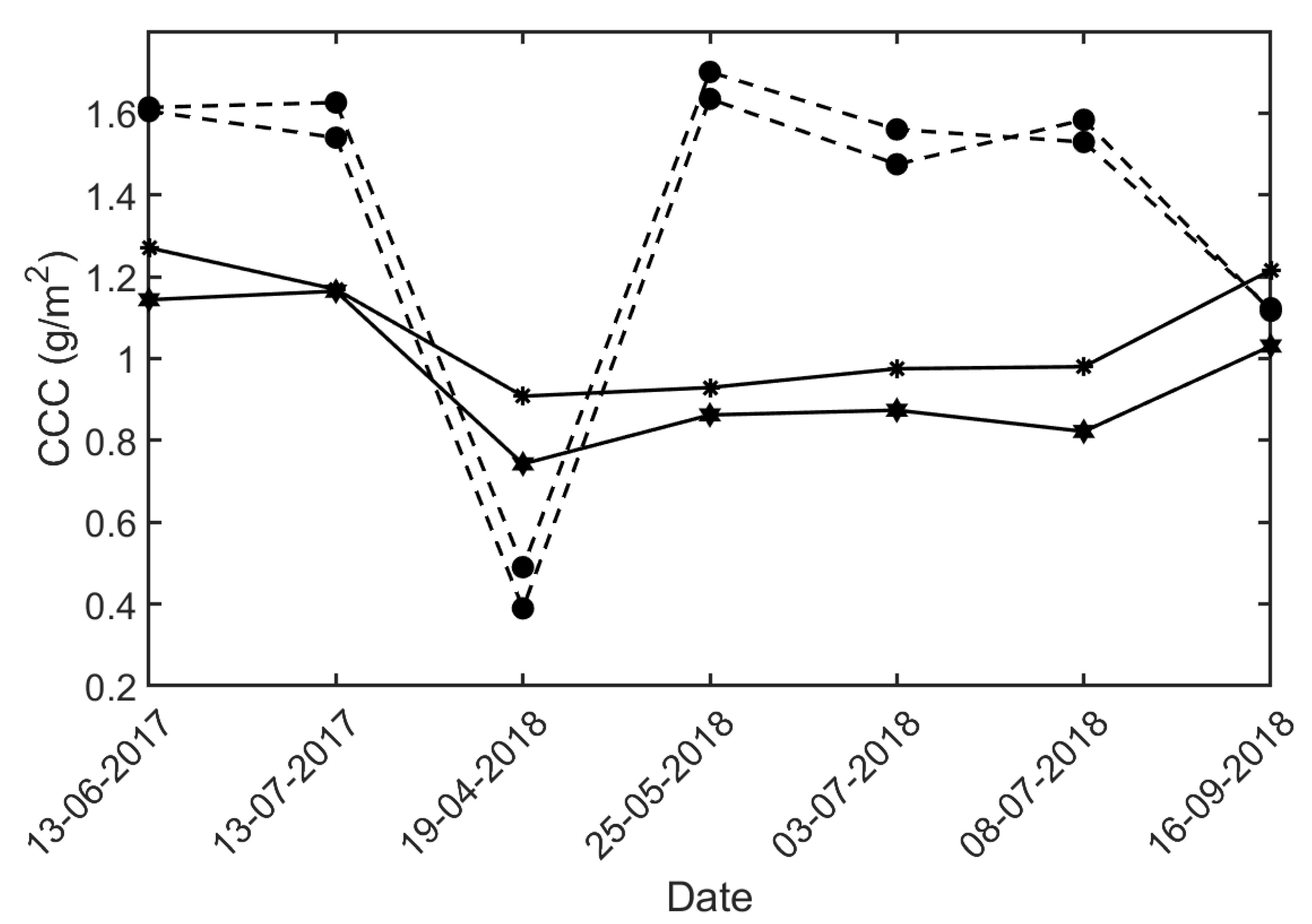
The selected methods were applied to a time series of Sentinel-2 imagery for the Bavarian Forest pilot site, as well as the short vegetation biome (La Camargue pilot site) in order to assess the consistency of the robustness of the methods through time. The seasonal variability of CCC in broadleaf and conifer stands of the Bavarian temperate forest is demonstrated in Figure 8. As expected, the variation in CCC is minimal in conifer stands compared to broadleaf.
Plotting the predictions made by the candidate algorithms in BFNP against each other for all the available image dates (seven dates) for randomly selected pixels to check if the relationship changes through time did not show a significant difference (Figure 9). The time series scatter plots have a similar pattern to the result obtained by applying the methods in single time Sentinel-2 data demonstrated in Figure 7a–c. Nonetheless, the INFORM inversion against the SNAP toolbox approach (Figure 9c) elucidated a higher correlation to the single date product (Figure 7c) than others (Figure 9a,b).
Similarly, we checked the temporal consistency of the obtained results in the La Camargue pilot site to understand whether the relationship between pairs of results changes through time. The PROSAIL inversion using LUT, SRVI, and the SNAP toolbox approaches were applied on 15 dates of Sentinel-2 data available for La Camargue between July 2017 and September 2018. The nature of the relationship between CCC predicted values does not change. Comparing the CCC prediction results from time series analysis (Figure 10) with single time prediction (Figure 7g–i) revealed temporal consistency between the predictions by PROSAIL and SRVI methods in the Mediterranean wetland ecosystem. However, the coefficient of determination significantly deteriorated when the prediction of the SNAP toolbox approach paired with other methods. Notably, the R2 between predictions of the SNAP toolbox and SRVI decreased from R2 = 0.90 in single date analysis (Figure 7g) to R2 = 0.61 in time series analysis (Figure 10a).

4. Discussion

Very little was found in the literature on the global canopy chlorophyll content (CCC) products from high spatial resolution remote sensing data. The present study was designed to determine the best-practice approach that may be implemented for mapping such CCC products through spatiotemporal consistency and robustness comparison across biomes.
One interesting finding is the spatial distribution of estimated CCC by the candidate algorithms displayed similar patterns in the BFNP, where calibration and validation of the methods were performed using an in situ dataset (Figure 2). Likewise, the violin plot (Figure 6) and the two-sample Kolmogorov-Smirnov test (Table 6) among pairs of CCC products proved the absence of significant spatial distribution disparities in this pilot site. These results are in line with previous findings [23,29], which showed the vigor of models when they are tuned for a particular biome.
However, some of the methods, mainly, PLSR, poorly performed in other biomes (Figure 4 and Figure 5). The possible explanation for the weak performance of the PLSR could be due to overfitting of non-parametric methods that stem from excessively multifaceted models that seize more than the underlying correlation [24,64]. This suggests that non-parametric methods are not well suited for global retrieval schemes. Although the PLSR performed well during validation using in situ data in Ali, Darvishzadeh [40], it posed a question about the transferability of the method across biomes. It demands calibration of PLSR for different biomes separately, and this is not feasible if it has to be implemented on an operational basis. Therefore, PLSR was not found suitable for large scale mapping, and thus we compared to the other three algorithms (i.e., the SNAP toolbox, SRVI, and INFORM/PROSAIL) for their operational feasibility through observing spatiotemporal consistency and robustness across biomes. Consistent with the literature, this research found that statistical methods are site and sensor-specific and rely on sampling circumstances, and may vary in space and over time [29,65].
The predictions made using SRVI and the SNAP toolbox approach, which is a combination of statistical and physical models, resulted in a systematic over/under-estimation of CCC when applied in different biomes. For instance, the SNAP toolbox approach [56] showed a tendency of overestimation, particularly in the wetland study site, when compared to SRVI and RTM inversion by LUT (Figure 7g–i). This result largely supports the finding of other authors [66,67,68] who highlighted the limitation of statistical methods in predicting vegetation variables from earth observation data.
In terms of predictive values agreement, all pairs of CCC products produced by the candidate approaches showed a good correlation. The highest correlation (R2 = 0.93) was observed between predictions of the SNAP toolbox and PROSAIL inversion by LUT (Figure 7i), and the weakest relationship (R2 = 0.57) was recorded in the tundra (Figure 7j). The weak agreements between predictions in the tundra may be partly due to the low chlorophyll content of tundra biomes, which is close to the minimum detectable CCC by several of the candidate methods. Weak relationships (R2 ≤ 0.43) between pigment content and spectral indices have also been reported by Beamish, et al. [69] in a low arctic tundra terrestrial ecosystem.
CCC predictions by INFORM and PROSAIL inversion by LUT exhibit ranges closer to expectations in three of the four biomes (Table 5), which implies that RTM approaches are rigorous. In many cases, lower disparities, higher R2, lower RMSE, and bias close to zero were observed when other methods compared with RTM inversions by LUT (Table 6, and Figure 7c,e,h,l), and reaffirmed the RTM based approaches applicability in different biomes. It is encouraging to compare this figure with that found by Ali, Darvishzadeh [40] who found that unlike the SRVI and the SNAP toolbox approach, RTM inversions by LUT provided a non-biased prediction.
Temporal consistency verification in the two pilot sites (Bavaria and La Camargue) also portrayed the robustness of the RTM based approaches. Pairwise comparison of the time series analysis products from INFORM inversion against SNAP toolbox approach (R2 = 0.88, RMSE = 0.25 g/m2) in temperate forest (Figure 9c), and PROSAIL inversion against SRVI (R2 = 0.88, RMSE = 0.19 g/m2) in the wetland site (Figure 10b) elucidated more similarity to the single date predictions shown in Figure 7c (R2 = 0.82, RMSE = 0.3 g/m2) and Figure 7h (R2 = 0.83, RMSE = 0.17 g/m2) respectively than others pairs, which reaffirms the fact that RTM based predictions are spatiotemporally consistent. These results are in accord with a recent study indicating that an RTM inversion is the robust method in the global mapping of the distribution of leaf chlorophyll content from ENVISAT MERIS full resolution (300 m) satellite imagery [39].
However, RTM inversion using LUTs requires a large set of input parameters at the leaf and canopy level to parameterize the models, and the models can be computationally expensive to execute. For instance, the inversion of INFORM took two solid days (result not shown) per pilot site. In contrast, the approach already implemented in the ESA SNAP toolbox and the parametric regression approach (i.e., SRVI) is easy and convenient to retrieve CCC from Earth observation data. It took less than one minute per pilot site. Thus, the SRVI and the SNAP toolbox approach may be the operationally more feasible approaches in terms of computation for the prediction of CCC from large remote sensing datasets. There is, therefore, a definite need for a trade-off between the accurate prediction of CCC globally and computational efficiency. Recent advances in computer science and cloud computing systems tremendously improved computational efficiency. This implies that the computationally demanding nature of RTMs inversion does not preclude them from being operationally feasible algorithms.

5. Conclusions

The purpose of this work was to determine the best-practice approach that can be implemented to map canopy chlorophyll content (CCC) across biomes from high spatial resolution remote sensing data. This study builds upon our earlier study, where the selected methods have been validated using existing in situ data [40]. In this study, we further compared their spatiotemporal consistency and robustness across different biomes to recommend the method(s) that suit for large-scale mapping of CCC from remote sensing data.
The major finding was that all methods exhibit spatiotemporal consistency. However, the statistical (e.g., SRVI) and hybrid (e.g., SNAP toolbox) approaches lead to a systematic over/under-estimation of CCC when applied in different biomes. CCC predictions by INFORM and PROSAIL inversion by LUT were rigorous and much closer to expected ranges. They were found non-biased and robust predictor across biomes. Therefore, based on the theoretical analysis of the rewards and drawbacks of the algorithms, spatiotemporal consistency across biomes, and robustness comparisons, the RTM inversion using LUT approach particularly INFORM for ‘forest’ and PROSAIL for ‘short vegetation’ ecosystems are recommended for large scale mapping of CCC from Sentinel-2 data. Future endeavors may include more rigorous validation of the CCC products obtained by the recommended approaches using field data collected for different terrestrial biomes.

Author Contributions

Conceptualization, A.M.A., A.S. and R.D.; methodology, A.M.A., A.S. and R.D.; software, A.M.A.; validation, A.M.A.; formal analysis, A.M.A.; investigation, M.P.; resources, A.S.; data curation, A.M.A.; writing—original draft preparation, A.M.A.; writing—review and editing, R.D., A.S., M.H., U.H. and S.M.; visualization, A.M.A.; supervision, A.S. and M.P.; project administration, A.S., R.D. and M.P.; funding acquisition, A.S. All authors have read and agreed to the published version of the manuscript.

Funding

This research received no external funding.

Acknowledgments

The authors would like to thank the four anonymous reviewers who provided helpful comments on earlier drafts of the manuscript.

Conflicts of Interest

The authors declare no conflict of interest.

References

  1. Murchie, E.H.; Lawson, T. Chlorophyll fluorescence analysis: A guide to good practice and understanding some new applications. J. Exp. Bot. 2013, 64, 3983–3998. [Google Scholar] [CrossRef] [PubMed] [Green Version]
  2. Lausch, A.; Erasmi, S.; King, D.J.; Magdon, P.; Heurich, M. Understanding forest health with remote sensing-part I—A review of spectral traits, processes and remote-sensing characteristics. Remote Sens. 2016, 8, 1029. [Google Scholar] [CrossRef] [Green Version]
  3. Houborg, R.; Cescatti, A.; Migliavacca, M.; Kustas, W.P. Satellite retrievals of leaf chlorophyll and photosynthetic capacity for improved modeling of GPP. Agric. For. Meteorol. 2013, 117, 10–23. [Google Scholar] [CrossRef]
  4. Peng, Y.; Gitelson, A.A. Application of chlorophyll-related vegetation indices for remote estimation of maize productivity. Agric. For. Meteorol. 2011, 151, 1267–1276. [Google Scholar] [CrossRef]
  5. Luo, X.; Croft, H.; Chen, J.M.; Bartlett, P.; Staebler, R.; Froelich, N. Incorporating leaf chlorophyll content into a two-leaf terrestrial biosphere model for estimating carbon and water fluxes at a forest site. Agric. For. Meteorol. 2018, 248, 156–168. [Google Scholar] [CrossRef] [Green Version]
  6. Wu, C.; Niu, Z.; Gao, S. The potential of the satellite derived green chlorophyll index for estimating midday light use efficiency in maize, coniferous forest and grassland. Ecol. Indic. 2012, 14, 66–73. [Google Scholar] [CrossRef]
  7. Dash, J.; Curran, P.J.; Foody, G.M. Remote sensing of terrestrial chlorophyll content. In Global Climatology and Ecodynamics; Springer: Berlin/Heidelberg, Germany, 2009; pp. 77–105. [Google Scholar]
  8. Korus, A. Effect of preliminary and technological treatments on the content of chlorophylls and carotenoids in kale (Brassica oleracea L. var. acephala). J. Food Process. Preserv. 2013, 37, 335–344. [Google Scholar] [CrossRef]
  9. Zhao, C.; Wang, Z.; Wang, J.; Huang, W.; Guo, T. Early detection of canopy nitrogen deficiency in winter wheat (Triticum aestivum L.) based on hyperspectral measurement of canopy chlorophyll status. N. Z. J. Crop Hortic. Sci. 2011, 39, 251–262. [Google Scholar] [CrossRef] [Green Version]
  10. Inoue, Y.; Guérif, M.; Baret, F.; Skidmore, A.; Gitelson, A.; Schlerf, M.; Darvishzadeh, R.; Olioso, A. Simple and robust methods for remote sensing of canopy chlorophyll content: A comparative analysis of hyperspectral data for different types of vegetation. Plant Cell Environ. 2016, 39, 2609–2623. [Google Scholar] [CrossRef] [Green Version]
  11. Abdullah, H.; Darvishzadeh, R.; Skidmore, A.K.; Groen, T.A.; Heurich, M. European spruce bark beetle (Ips typographus L.) green attack affects foliar reflectance and biochemical properties. Int. J. Appl. Earth Obs. Geoinf. 2018, 64, 199–209. [Google Scholar] [CrossRef] [Green Version]
  12. Secretariat of CBD. Global Biodiversity Outlook 3; Progress Press Ltd: Malta, 2010.
  13. Skidmore, A.K.; Pettorelli, N.; Coops, N.C.; Geller, G.N.; Hansen, H.; Lucas, R.; Mücher, C.A.; O’Connor, B.; Paganini, M.; Pereira, H.M.; et al. Agree on biodiversity metrics to track from space. Nature 2015, 523, 403–405. [Google Scholar] [CrossRef] [Green Version]
  14. Vincini, M.; Calegari, F.; Casa, R. Sensitivity of leaf chlorophyll empirical estimators obtained at Sentinel-2 spectral resolution for different canopy structures. Precis. Agric. 2016, 17, 313–331. [Google Scholar] [CrossRef]
  15. Dian, Y.; Le, Y.; Fang, S.; Xu, Y.; Yao, C.; Liu, G. Influence of Spectral Bandwidth and Position on Chlorophyll Content Retrieval at Leaf and Canopy Levels. J. Indian Soc. Remote Sens. 2016, 44, 583–593. [Google Scholar] [CrossRef]
  16. Li, X.; Liu, X.; Liu, M.; Wang, C.; Xia, X. A hyperspectral index sensitive to subtle changes in the canopy chlorophyll content under arsenic stress. Int. J. Appl. Earth Obs. Geoinf. 2015, 36, 41–53. [Google Scholar] [CrossRef]
  17. Ma, M.; Shi, R.; Liu, P.; Wang, H.; Gao, W. The impacts of bandwidths on the estimation of leaf chlorophyll concentration using normalized difference vegetation indices. In Proceedings of the SPIE—The International Society for Optical Engineering, San Diego, CA, USA, 17–21 August 2014. [Google Scholar]
  18. Verrelst, J.; Muñoz, J.; Alonso, L.; Delegido, J.; Rivera, J.P.; Camps-Valls, G.; Moreno, J. Machine learning regression algorithms for biophysical parameter retrieval: Opportunities for Sentinel-2 and -3. Remote Sens. Environ. 2012, 118, 127–139. [Google Scholar] [CrossRef]
  19. Okuda, K.; Taniguchi, K.; Miura, M.; Obata, K.; Yoshioka, H. Application of vegetation isoline equations for simultaneous retrieval of leaf area index and leaf chlorophyll content using reflectance of red edge band. In Proceedings of the SPIE—The International Society for Optical Engineering, San Diego, CA, USA, 28 August–1 September 2016. [Google Scholar]
  20. Li, L.; Ren, T.; Ma, Y.; Wei, Q.; Wang, S.; Li, X.; Cong, R.; Liu, S.; Lu, J. Evaluating chlorophyll density in winter oilseed rape (Brassica napus L.) using canopy hyperspectral red-edge parameters. Comput. Electron. Agric. 2016, 126, 21–31. [Google Scholar] [CrossRef]
  21. Curran, P.J. Remote-Sensing of Foliar Chemistry. Remote Sens. Environ. 1989, 30, 271–278. [Google Scholar] [CrossRef]
  22. Baret, F.; Buis, S. Estimating canopy characteristics from remote sensing observations: Review of methods and associated problems. In Advances in Land Remote Sensing: System, Modeling, Inversion and Application; Springer: Dordrecht, The Netherlands, 2008. [Google Scholar]
  23. Darvishzadeh, R.; Skidmore, A.; Schlerf, M.; Atzberger, C.; Corsi, F.; Cho, M. LAI and chlorophyll estimation for a heterogeneous grassland using hyperspectral measurements. ISPRS J. Photogramm. Remote Sens. 2008, 63, 409–426. [Google Scholar] [CrossRef]
  24. Verrelst, J.; Camps-Valls, G.; Muñoz-Marí, J.; Rivera, J.P.; Veroustraete, F.; Clevers, J.G.P.W.; Moreno, J. Optical remote sensing and the retrieval of terrestrial vegetation bio-geophysical properties—A review. ISPRS J. Photogramm. Remote Sens. 2015, 108 (Suppl. C), 273–290. [Google Scholar] [CrossRef]
  25. Asner, G.P. Biophysical and biochemical sources of variability in canopy reflectance (vol 64, pg 234, 1997). Remote Sens. Environ. 1998, 65, 225–226. [Google Scholar]
  26. Gitelson, A.A.; Viña, A.; Ciganda, V.; Rundquist, D.C.; Arkebauer, T.J. Remote estimation of canopy chlorophyll content in crops. Geophys. Res. Lett. 2005, 32. [Google Scholar] [CrossRef] [Green Version]
  27. Schlerf, M.; Atzberger, C. Inversion of a forest reflectance model to estimate structural canopy variables from hyperspectral remote sensing data. Remote Sens. Environ. 2006, 100, 281–294. [Google Scholar] [CrossRef]
  28. Jacquemoud, S.; Verhoef, W.; Baret, F.; Bacour, C.; Zarco-Tejada, P.J.; Asner, G.P.; Francois, C.; Ustin, S.L. PROSPECT plus SAIL models: A review of use for vegetation characterization. Remote Sens. Environ. 2009, 113, S56–S66. [Google Scholar] [CrossRef]
  29. Colombo, R.; Bellingeri, D.; Fasolini, D.; Marino, C.M. Retrieval of leaf area index in different vegetation types using high resolution satellite data. Remote Sens. Environ. 2003, 86, 120–131. [Google Scholar] [CrossRef]
  30. Xie, Y.; Sha, Z.; Yu, M. Remote sensing imagery in vegetation mapping: A review. J. Plant Ecol. 2008, 1, 9–23. [Google Scholar] [CrossRef]
  31. Croft, H.; Chen, J.M.; Zhang, Y. The applicability of empirical vegetation indices for determining leaf chlorophyll content over different leaf and canopy structures. Ecol. Complex. 2014, 17, 119–130. [Google Scholar] [CrossRef]
  32. Blackburn, G.A. Quantifying chlorophylls and caroteniods at leaf and canopy scales: An evaluation of some hyperspectral approaches. Remote Sens. Environ. 1998, 66, 273–285. [Google Scholar] [CrossRef]
  33. Ustin, S.L.; Gitelson, A.A.; Jacquemoud, S.; Schaepman, M.; Asner, G.P.; Gamon, J.A.; Zarco-Tejada, P. Retrieval of foliar information about plant pigment systems from high resolution spectroscopy. Remote Sens. Environ. 2009, 113 (Suppl. 1), S67–S77. [Google Scholar] [CrossRef] [Green Version]
  34. Ollinger, S.V. Sources of variability in canopy reflectance and the convergent properties of plants. New Phytol. 2011, 189, 375–394. [Google Scholar] [CrossRef]
  35. Zheng, G.; Moskal, L.M. Retrieving Leaf Area Index (LAI) Using Remote Sensing: Theories, Methods and Sensors. Sensors 2009, 9, 2719–2745. [Google Scholar] [CrossRef] [Green Version]
  36. Chen, J.; Chen, J.; Liao, A.; Cao, X.; Chen, L.; Chen, X.; He, C.; Han, G.; Peng, S.; Lu, M.; et al. Global land cover mapping at 30m resolution: A POK-based operational approach. ISPRS J. Photogramm. Remote Sens. 2015, 103, 7–27. [Google Scholar] [CrossRef] [Green Version]
  37. Dash, J.; Curran, P.J. The MERIS terrestrial chlorophyll index. Int. J. Remote Sens. 2004, 25, 5403–5413. [Google Scholar] [CrossRef]
  38. Dash, J.; Vuolo, F. Algorithm Theoretical Basis Document: OLCI Terrestrial Chlorophyll Index (OTCI); University of Southampton: Southampton, UK, 2010. [Google Scholar]
  39. Croft, H.; Chen, J.M.; Wang, R.; Mo, G.; Luo, S.; Luo, X.; He, L.; Gonsamo, A.; Arabian, J.; Zhang, Y.; et al. The global distribution of leaf chlorophyll content. Remote Sens. Environ. 2020, 236, 111479. [Google Scholar] [CrossRef]
  40. Ali, A.M.; Darvishzadeh, R.; Skidmore, A.; Gara, T.W.; O’Connor, B.; Roeoesli, C.; Heurich, M.; Paganini, M. Comparing methods for mapping canopy chlorophyll content in a mixed mountain forest using Sentinel-2 data. Int. J. Appl. Earth Obs. Geoinf. 2020, 87, 102037. [Google Scholar] [CrossRef]
  41. Nauta, A.L.; Heijmans, M.M.; Blok, D.; Limpens, J.; Elberling, B.; Gallagher, A.; Li, B.; Petrov, R.E.; Maximov, T.C.; Van Huissteden, J. Permafrost collapse after shrub removal shifts tundra ecosystem to a methane source. Nat. Clim. Chang. 2015, 5, 67–70. [Google Scholar] [CrossRef]
  42. Blok, D.; Heijmans, M.M.; Schaepman-strub, G.; Kononov, A.; Maximov, T.; Berendse, F. Shrub expansion may reduce summer permafrost thaw in Siberian tundra. Glob. Chang. Biol. 2010, 16, 1296–1305. [Google Scholar] [CrossRef]
  43. Blondel, J.; Barruol, G.; Vianet, R. L’Encyclopédie de la Camargue; Buchet-Chastel: Paris, France, 2013. [Google Scholar]
  44. Dehorter, O.; Tamisier, A. Wetland habitat characteristics for waterfowl wintering in Camargue, Southern France: Implications for conservation. Revue d’écologie 1996, 51, 161–172. [Google Scholar]
  45. Heurich, M.; Beudert, B.; Rall, H.; Křenová, Z. National Parks as Model Regions for Interdisciplinary Long-Term Ecological Research: The Bavarian Forest and Šumavá National Parks Underway to Transboundary Ecosystem Research. In Long-Term Ecological Research: Between Theory and Application; Müller, F., Baessler, C., Schubert, H., Klotz, S., Eds.; Springer: Dordrecht, The Netherlands, 2010; pp. 327–344. [Google Scholar]
  46. Cailleret, M.; Heurich, M.; Bugmann, H. Reduction in browsing intensity may not compensate climate change effects on tree species composition in the Bavarian Forest National Park. For. Ecol. Manag. 2014, 328, 179–192. [Google Scholar] [CrossRef]
  47. Kumagai, T.O.; Saitoh, T.M.; Sato, Y.; Morooka, T.; Manfroi, O.J.; Kuraji, K.; Suzuki, M. Transpiration, canopy conductance and the decoupling coefficient of a lowland mixed dipterocarp forest in Sarawak, Borneo: Dry spell effects. J. Hydrol. 2004, 287, 237–251. [Google Scholar] [CrossRef]
  48. Atzberger, C. Development of an invertible forest reflectance model: The INFOR-model. Decade Trans-Eur. Remote Sens. Coop. 2001, 01, 39–44. [Google Scholar]
  49. Wang, Z.; Skidmore, A.K.; Wang, T.; Darvishzadeh, R.; Heiden, U.; Heurich, M.; Latifi, H.; Hearne, J. Canopy foliar nitrogen retrieved from airborne hyperspectral imagery by correcting for canopy structure effects. Int. J. Appl. Earth Obs. Geoinf. 2017, 54, 84–94. [Google Scholar] [CrossRef]
  50. Darvishzadeh, R.; Skidmore, A.; Abdullah, H.; Cherenet, E.; Ali, A.; Wang, T.; Nieuwenhuis, W.; Heurich, M.; Vrieling, A.; O’Connor, B.; et al. Mapping leaf chlorophyll content from Sentinel-2 and RapidEye data in spruce stands using the invertible forest reflectance model. Int. J. Appl. Earth Obs. Geoinf. 2019, 79, 58–70. [Google Scholar] [CrossRef] [Green Version]
  51. Atzberger, C.; Darvishzadeh, R.; Immitzer, M.; Schlerf, M.; Skidmore, A.; le Maire, G. Comparative analysis of different retrieval methods for mapping grassland leaf area index using airborne imaging spectroscopy. Int. J. Appl. Earth Obs. Geoinf. 2015, 43, 19–31. [Google Scholar] [CrossRef] [Green Version]
  52. Darvishzadeh, R.; Skidmore, A.; Schlerf, M.; Atzberger, C. Inversion of a radiative transfer model for estimating vegetation LAI and chlorophyll in a heterogeneous grassland. Remote Sens. Environ. 2008, 112, 2592–2604. [Google Scholar] [CrossRef]
  53. Atzberger, C.; Darvishzadeh, R.; Schlerf, M.; Le Maire, G. Suitability and adaptation of PROSAIL radiative transfer model for hyperspectral grassland studies. Remote Sens. Lett. 2013, 4, 56–65. [Google Scholar] [CrossRef]
  54. Ali, A.M.; Darvishzadeh, R.; Skidmore, A.K.; van Duren, I.; Heiden, U.; Heurich, M. Estimating leaf functional traits by inversion of PROSPECT: Assessing leaf dry matter content and specific leaf area in mixed mountainous forest. Int. J. Appl. Earth Obs. Geoinf. 2016, 45, 66–76. [Google Scholar] [CrossRef] [Green Version]
  55. Ali, A.M.; Skidmore, A.K.; Darvishzadeh, R.; van Duren, I.; Holzwarth, S.; Mueller, J. Retrieval of forest leaf functional traits from HySpex imagery using radiative transfer models and continuous wavelet analysis. ISPRS J. Photogramm. Remote Sens. 2016, 122, 68–80. [Google Scholar] [CrossRef] [Green Version]
  56. S2ToolBox Level 2 products: LAI, FAPAR, FCOVER: ATBD used to compute LAI, FAPAR and FVC, from SENTINEL2 top of canopy reflectance data that is implemented in the SENTINEL2 Toolbox. Available online: https://step.esa.int/docs/extra/ATBD_S2ToolBox_L2B_V1.1.pdf (accessed on 30 May 2020).
  57. Féret, J.B.; Gitelson, A.A.; Noble, S.D.; Jacquemoud, S. PROSPECT-D: Towards modeling leaf optical properties through a complete lifecycle. Remote Sens. Environ. 2017, 193, 204–215. [Google Scholar] [CrossRef] [Green Version]
  58. Yin, C.; He, B.; Quan, X.; Liao, Z. Chlorophyll content estimation in arid grasslands from Landsat-8 OLI data. Int. J. Remote Sens. 2016, 37, 615–632. [Google Scholar] [CrossRef]
  59. Massey, F.J. The Kolmogorov-Smirnov Test for Goodness of Fit. J. Am. Stat. Assoc. 1951, 46, 68–78. [Google Scholar] [CrossRef]
  60. Singh, D.; Singh, S. Geospatial Modeling of Canopy Chlorophyll Content Using High Spectral Resolution Satellite Data in Himalayan Forests. Clim. Chang. Environ. Sustain. 2018, 6, 20–34. [Google Scholar] [CrossRef]
  61. Asner, G.P.; Scurlock, J.M.O.; Hicke, J.A. Global synthesis of leaf area index observations: Implications for ecological and remote sensing studies. Glob. Ecol. Biogeogr. 2003, 12, 191–205. [Google Scholar] [CrossRef] [Green Version]
  62. Lee, H.S.; Davies, S.J.; LaFrankie, J.V.; Tan, S.; Yamakura, T.; Itoh, A.; Ohkubo, T.; Ashton, P.S. Floristic and structural diversity of mixed dipterocarp forest in lambir hills national park, sarawak, malaysia. J. Trop. For. Sci. 2002, 14, 379–400. [Google Scholar]
  63. Tieszen, L.L. Comparisons of Chlorophyll Content and Leaf Structure in Arctic and Alpine Grasses. Am. Midl. Nat. 1970, 83, 238–253. [Google Scholar] [CrossRef]
  64. Rocha, A.D.; Groen, T.A.; Skidmore, A.K.; Darvishzadeh, R.; Willemen, L. The Naïve Overfitting Index Selection (NOIS): A new method to optimize model complexity for hyperspectral data. ISPRS J. Photogramm. Remote Sens. 2017, 133 (Suppl. C), 61–74. [Google Scholar] [CrossRef]
  65. Baret, F.; Guyot, G.; Major, D.J. Crop Biomass Evaluation Using Radiometric Measurements. Photogrammetria 1989, 43, 241–256. [Google Scholar] [CrossRef]
  66. Ali, A.M.; Darvishzadeh, R.; Shahi, K.R.; Skidmore, A. Validating the Predictive Power of Statistical Models in Retrieving Leaf Dry Matter Content of a Coastal Wetland from a Sentinel-2 Image. Remote Sens. 2019, 11, 1936. [Google Scholar] [CrossRef] [Green Version]
  67. Sun, Q.; Jiao, Q.J.; Dai, H.Y. Evaluating the capabilities of vegetation spectral indices on chlorophyll content estimation at Sentinel-2 spectral resolutions. In Mippr 2017: Remote Sensing Image Processing, Geographic Information Systems, and Other Applications; SPIE: Bellingham, WA, USA, 2018; Volume 10611. [Google Scholar]
  68. Houborg, R.; McCabe, M.F. A hybrid training approach for leaf area index estimation via Cubist and random forests machine-learning. Isprs J. Photogramm. Remote Sens. 2018, 135, 173–188. [Google Scholar] [CrossRef]
  69. Beamish, A.L.; Coops, N.C.; Hermosilla, T.; Chabrillat, S.; Heim, B. Monitoring pigment-driven vegetation changes in a low-Arctic tundra ecosystem using digital cameras. Ecosphere 2018, 9, e02123. [Google Scholar] [CrossRef] [Green Version]
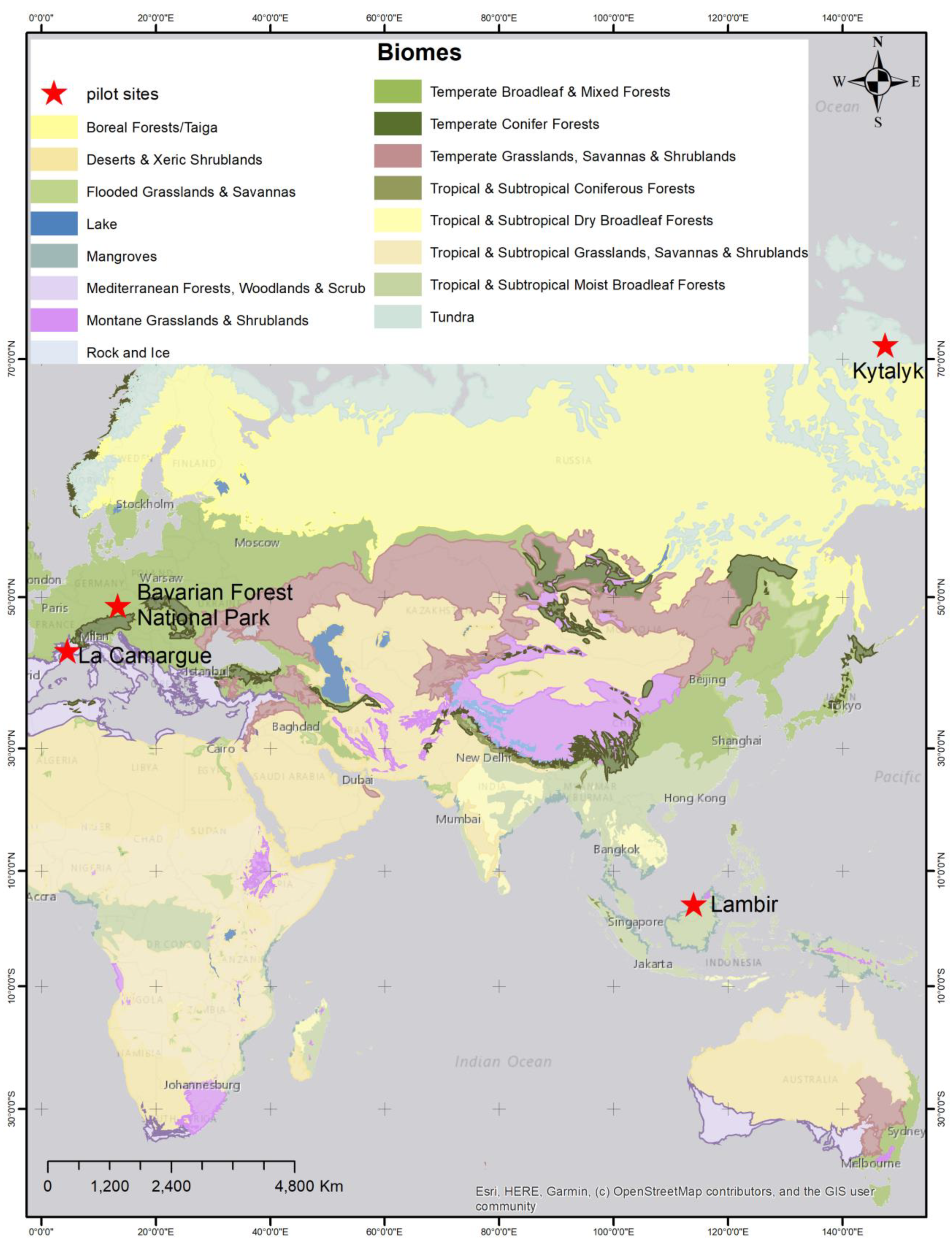
Figure 1. The four selected pilot sites from terrestrial biomes.
Remotesensing 12 01788 g001
Figure 2. CCC products derived from the Sentinel-2 image acquired on 17 July 2017 over Bavaria Forest National Park by running the SNAP toolbox (a), SRVI (b), INFORM (c), and PLSR (d). CCC is higher in deciduous stands than conifers.
Remotesensing 12 01788 g002
Figure 3. CCC map predicted from 28 June 2017 Sentinel-2 data using the candidate algorithms for the Lambir pilot site (tropical forest). the SNAP toolbox (a), SRVI (b), INFORM (c), and PLSR (d).
Remotesensing 12 01788 g003
Figure 4. CCC products retrieved from Sentinel-2 image of 19 July 2018, by running the SNAP toolbox (a), SRVI (b), PROSAIL (c), and PLSR (d) for the La Camargue pilot site.
Remotesensing 12 01788 g004
Figure 5. CCC products estimated from the Sentinel-2 image of 21 May 2018, using the SNAP toolbox (a), SRVI (b), PROSAIL inversion by LUT (c), and PLSR (d) for the Kytalyk Arctic tundra pilot site.
Remotesensing 12 01788 g005
Figure 6. Violin plots of predicted CCC (g/m2), showing the differences in frequency distribution among four biomes; (a) temperate forest, (b) wetland, (c) tropical forest, and (d) arctic tundra. The square and the plus sign indicate the median and mean of the predicted CCC by each method.
Remotesensing 12 01788 g006
Figure 7. Robustness of the selected approaches against each other in predicting CCC of Bavarian temperate forest (a–c), Lambir tropical forest (d–f), Camargue Mediterranean wetland (g–i), and Kytalyk arctic tundra biome (j–l). The lines in black show the 1:1 relationship, whereas the lines in red indicate the relationship between the estimated CCC values by the tested algorithms.
Remotesensing 12 01788 g007
Figure 8. Seasonal variability of CCC between June 2017 and September 2018 in the Bavarian Forest National Park. The broken lines show the seasonal variation in broadleaf stands, and the solid lines in a conifer stand for randomly selected two pixels.
Remotesensing 12 01788 g008
Figure 9. The goodness of fit between CCC values predicted by SRVI vs. SNAP toolbox (a), INFORM inversion vs. SRVI (b), and INFORM inversion vs. SNAP toolbox (c) for seven dates of Sentinel-2 data available for BFNP. The lines in black show the 1:1 relationship, whereas the lines in red, demonstrate the relationship between the CCC estimates by the selected algorithms.
Remotesensing 12 01788 g009
Figure 10. The goodness of fit between CCC predicted values by SRVI vs. SNAP toolbox (a), PROSAIL inversion vs. SRVI (b), and PROSAIL inversion vs. SNAP toolbox (c) for 15 dates of Sentinel-2 data available for the La Camargue pilot site. The lines in black show the 1:1 relationship, whereas the lines in red, designates the relationship between the CCC estimates by the selected algorithms.
Remotesensing 12 01788 g010
Table 1. Tiles and acquisition dates of the downloaded Sentinel-2 images for the four pilot sites.
Pilot SiteSentinel-2 Tile NumberNo. ImagesDate of Acquisition
KytalykT55WEU121 May 2018
La CamargueT31TFJ15(29 July, 18 August, 7 & 8 September, 27 October & 24 December) 2017
(26 March, 25 April, 25 May, 19 &27 June, 27 July, 16 August & 27 September) 2018
Bavarian Forest National parkT33UUQ7(13 June & 13 July) 2017
(19 April, 29 May, 3 & 8 July) 2018
LambirT49NHE128 June 2018
Table 2. Specifications of the Sentinel-2 multi-spectral instrument (MSI).
Spectral BandFunctionCenter Wavelength (nm)Band Width (nm)Spatial Resolution (m)
B1Coastal aerosol4432160
B2Blue4906610
B3Green5603610
B4Red6653110
B5Vegetation red edge7051520
B6Vegetation red edge7401520
B7Vegetation red edge7832020
B8Near Infrared (NIR)84210610
B8aNIR8652220
B9Water vapor9402160
B10SWIR-Cirrus13753160
B11Short wave infrared (SWIR)16109320
B12SWIR219018020
Table 3. INFORM input parameters used to build the LUT. The inputs were defined through the literature review and sensor configuration of Sentinel-2.
ParameterSymbolUnitRange or Fixed ValuesReference
MinMax
Leaf dry mass per areaCmg/cm20.0050.03[54]
Equivalent water thicknessCwg/cm20.0060.035[54]
Leaf structural parameterNNA12.5[54]
Leaf chlorophyll contentCabµg/cm2565[40]
Single tree LAILAIsNA210[55]
Understory LAILAIuNA0.21[40]
Stem densitySDn/hr2002000[55]
Stand heightS.H.m540[55]
Crown diameterCDm310[55]
Average leaf angleALAdegree4060[55]
Sun zenith angleθsdegree2535Sentinel-2 metadata
Observation zenith angleθ0degree015Sentinel-2 metadata
Azimuth angleΦdegree50210Sentinel-2 metadata
Scale NA0.51.5[27]
Fraction of diffused radiationSky1fraction0.1[27]
Table 4. PROSAIL radiative transfer model input parameters used to build the look-up table (LUT) and the corresponding values for wetland, taiga, and tundra biomes.
ParameterSymbolUnitRange or fixed ValuesReference
MinMax
Leaf dry mass per areaCmg/cm20.0030.025[54]
Equivalent water thicknessCwg/cm20.0050.035[54]
Leaf structural parameterN 1.22.2[54]
Chlorophyll contentCabµg/cm2570[56]
Carotenoid contentCarµg/cm28 [57]
Anthocyanin contentAntµg/cm20 [57]
brown pigment contentCbrown 0 [57]
Leaf area indexLAIm2/m20.28[56]
Leaf inclination distribution function typeTypeLidf 2[57]
Leaf inclination distribution function aLIDFadegree2070[56]
Leaf inclination distribution function bLIDFb 0[57]
Hot spot factorHspot 0.5/LAI[58]
Soil reflectance factorpsoil 0.30.6[57]
Sun zenith angletsdegree2535Sentinel-2 metadata
Observation zenith anglet0degree015Sentinel-2 metadata
Azimuth anglepsidegree50210Sentinel-2 metadata
Table 5. Expected CCC range in each biome obtained from previous studies [10,60,61,62,63] and CCC ranges predicted by the candidate algorithms. Cells in bold show predicted CCC ranges by candidate methods nearer to expectation.
BiomeExpected CCC Range (g/m2)The Range of CCC Predicted by the Selected Methods
SRVISNAPINFORMPLSRPROSAIL
Temperate forest0.5–3.00.26–2.800.22–4.350.50–2.700.01–3.54
Tropical forest0.54–4.430.31–1.950.16–3.200.50–2.600.00–3.06
Wetland and crops0.0–6.00.19–2.000.03–7.16 0.05–2.820.08–4.12
Tundra0.004–0.40.32–1.640.01–2.34 0.03–2.080.05–1.52
Table 6. Results of paired t-test and Kolmogorov-Smirnov test (p = 0.01) to measure the mean difference in CCC and spatial distribution disparities among pairs of CCC products, respectively.
Bavarian Forest National Park (Temperate Forest)
Pair of MethodsPaired t-TestKolmogorov-Smirnov Test
Hp-Valuet-StatsSd.Hp-ValueK Stats
INFORM vs SRVI10.0092.660.412300.02180.1982
INFORM vs SNAP10.0010.280.246100.02180.1982
SRVI vs SNAP00.19291.310.26600.62440.0991
Lambir (Tropical forest)
INFORM vs. SRVI00.8894−0.140.35710.000.3468
INFORM vs. SNAP10.0012.190.422210.000.6532
SRVI vs. SNAP10.0024.560.211610.000.75
La Camargue (Wetland)
PROSAIL vs. SRVI10.00−5.290.138900.10340.2167
PROSAIL vs. SNAP10.00−14.310.208410.00400
SRVI vs. SNAP10.008.880.253210.0020.3333
Kytalyk (Arctic Tundra)
PROSAIL vs. SRVI10.0019.810.117210.000.91
PROSAIL vs. SNAP10.0012.190.137110.000.6911
SRVI vs. SNAP00.0138−16.400.039600.35110.1119