Evaluation of Cotton Emergence Using UAV-Based Narrow-Band Spectral Imagery with Customized Image Alignment and Stitching Algorithms

Abstract

Crop stand count and uniformity are important measures for making proper field management decisions to improve crop production. Conventional methods for evaluating stand count based on visual observation are time consuming and labor intensive, making it difficult to adequately cover a large field. The overall goal of this study was to evaluate cotton emergence at two weeks after planting using unmanned aerial vehicle (UAV)-based high-resolution narrow-band spectral indices that were collected using a pushbroom hyperspectral imager flying at 50 m above ground. A customized image alignment and stitching algorithm was developed to process hyperspectral cubes efficiently and build panoramas for each narrow band. The normalized difference vegetation index (NDVI) was calculated to segment cotton seedlings from soil background. A Hough transform was used for crop row identification and weed removal. Individual seedlings were identified based on customized geometric features and used to calculate stand count. Results show that the developed alignment and stitching algorithm had an average alignment error of 2.8 pixels, which was much smaller than that of 181 pixels from the associated commercial software. The system was able to count the number of seedlings in seedling clusters with an accuracy of 84.1%. Mean absolute percentage error (MAPE) in estimation of crop density at the meter level was 9.0%. For seedling uniformity evaluation, the MAPE of seedling spacing was 9.1% and seedling spacing standard deviation was 6.8%. Results showed that UAV-based high-resolution narrow-band spectral images had the potential to evaluate cotton emergence.

1. Introduction

Crop stand count and seedling development status, such as vigor, are important agronomic factors to assess crop emergence [1]. The evaluation of crop emergence can allow making timely and proper field management decisions in seedling stage. For example, the decision of replanting cotton (Gossypium hirsutum L.) is often made based on plant population (stand count), density and uniformity of seedlings [2,3]. Conventional methods to assess crop stand count and seedling vigor rely on visual observation by farmers or scientists that is time-consuming, labor-intensive, and not feasible when evaluating large production fields. Crop emergence in a production field is usually assessed by measuring plants in randomly-selected sampling areas, which is not accurate [4]. There is a pressing need to develop an efficient tool that can quickly and accurately evaluate stand count and uniformity for timely field management decision making.

Image sensing technology is promising to address the challenges in efficient and accurate evaluation of crop stand and seedling development status. Ground vehicles equipped with high-resolution image sensors have been used to evaluate crop emergence, including crop stand and health in early stages [5,6,7]. Although ground-based images are promising in monitoring small-size seedlings, they are inefficient to collect data in large production fields. Unmanned aerial vehicle (UAV)-based imaging systems have been used as a high-throughput tool to collect field data in different research and commercial applications. Researchers have been using UAVs equipped with RGB (red-green-blue) cameras to estimate wheat density [8] by estimating the overall number of crop pixels, to evaluate stand count for cotton [9], corn [10], and rapeseed [11] based on morphological features of crop leaves, and to evaluate rice stand count using a deep learning model [12]. Crop seedlings are relatively small in size and require a fine ground sample distance (GSD) for identification and segmentation of single plants from images. Therefore, UAV-based imaging systems usually fly at a very low altitude (e.g., 5–10 m above ground level, AGL) and slow speed to obtain sufficient numbers of pixels of plants.

Table 1. A brief summary of studies for crop emergence assessment using unmanned aerial vehicle (UAV)-based imagery.

Camera	Crop and Purpose	DAP (Days)	Imaging Height (m)	GSD (cm/pixel)	Performance	Reference
RGB	Wheat, uniformity	110 and 111	7	0.06	RMSE = 0.44–3.99	[6]
RGB	Wheat, stand count	14, 31 and 40	3–7	0.08–0.18	RMSE = 14.3%	[8]
RGB	Cotton, stand count	6–11	15–20	0.63–0.89	Accuracy = 88.6%	[9]
RGB	Corn, stand count	20 and 23	10	0.24	Accuracy = 96.0%	[10]
RGB	Rapeseed, stand count	27–37	20	0.41	MAE = 9.8%, MAE = 5.1%	[11]
RGB	Rice stand count	13	20	0.55	Accuracy = 93.36%	[12]
RGB	Sorghum, population	Not mentioned	40	Not mentioned	MAE = 6.7%	[13]
RGB	Potato, stand count	35	30	0.5	Accuracy = 96.6%	[14]
RGB	Maize, stand count	3- to 5-leaf stage	50	1.4	R2 = 0.89	[15]
RGB and Multispectral	Angustifolia seedling detection	68–92	5	RGB: 0.1, multispectral: 0.46	Only reported VIs were significant through time	[16]
RGB	Angustifolia seedling classification	1, 25, 68	5, 10, 15	0.1, 0.26, 0.4	Accuracy > 80.0%	[17]
Multispectral	Wheat, stand count	40 and 236	100	3.00	r = 0.86–0.87	[18]
Multispectral	Potato, stand count	32, 37 and 43	15	0.44	r = 0.82	[19]

Abbreviations: RGB = red, green and blue; DAP=days after planting; GSD = ground sample distance; VIs = vegetation indices; MAE = mean absolute error; RMSE = root mean square error; r = Pearson correlation coefficient.

summarizes the platforms and sensors that have been used in some recent studies for the evaluation of crop emergence based on UAV-based imaging systems, including image collection time, flight height, image resolution, and accuracy in estimation of stand count.

It can be seen from the table that the majority of the studies used RGB cameras to estimate stand count [8,9,10,11,15,19]. However, crop color in UAV images is affected by soil reflectance and is distorted when the proportion of soil in the image is high [20]. The reduction in contrast between crops and soil creates some challenges for segmentation and identification of cotton seedlings. To improve image quality, high-resolution (4K or 8K) cameras have been used in research [14,15]. For example, the studies of [16] and [17] showed the potential of using a UAV-based RGB camera (20 M pixel) for seedling detection.

Previous research [11] indicated that visible images were potentially affected by sunlight conditions [21] and suggested that using multispectral images with near infrared (NIR) spectral bands could be more efficient for crop segmentation. Multispectral images have been used to assess crop emergence using vegetation indices (VIs), such as the normalized difference vegetation index (NDVI) and green normalized difference vegetation index (GNDVI) [18,19]. However, most commercial multispectral cameras have low image resolution, ranging around 1–2 M pixels. Examples are the Micasense RedEdge-M (Micasense Inc., Seattle, WA, USA) and the Parrot Sequoia (Parrot SA Inc., Paris, France), each of which have 1.2 M pixel resolution [22]. A few customized multispectral cameras that are made by replacing the filter of one of the channels of a high-resolution RGB camera with a near-infrared filter (e.g., XNiteCanonElph130 used in [18,19]) have relatively higher resolution (e.g., 12 M pixel) and low cost. Those cameras have been successfully used in crop yield estimation [23], crop stress monitoring [24,25] and high throughput phenotyping [26]. These studies focused on areas or plots within fields at middle or late crop growth stages, where needs may be different from those for crop seedling studies. The customized multispectral cameras have broad spectral bands (e.g., around 80–100 nm for the XNiteCanonElph130) similar to those of the original cameras, and have same issues of color distortion, incorrect focus and small dynamic range [23] when they are used in seedling studies. Approaches to improve the quality of images may include collecting data at lower altitude [27] or combining VIs with a digital surface model (DSM) [28]. Studies also found that crop detection accuracy could be improved by selection of suitable VIs. The green-red vegetation index (GRVI) [29,30] and the wide-dynamic-range vegetation index (WDRVI) [31] showed promising results compared to the widely used NDVI and may be considered for seedling detection studies.

High-resolution narrow-band spectral images from a pushbroom hyperspectral camera were used for seeding evaluation in this study to address the pertinent challenges of color distortion of RGB cameras and low-resolution spectral cameras. However, the application of UAV-based pushbroom hyperspectral cameras is challenging, partly due to the difficulty in alignment and stitching of line-scanned images. Pushbroom hyperspectral imagers acquire data by scanning targeted objects line by line [32] while moving at a consistent speed relative to the target objects. Any speed variation may cause shifts in different bands during scanning and moving (flying), which may result in different spatial areas being sensed by different spectral bands [33]. Pushbroom hyperspectral imaging systems may improve the accuracy of alignment and stitching by using a high-performance GPS and inertial measurement unit (IMU) to track the variations of speed, pitch, roll and yaw angles of the imagers [34], or by using other sensors (i.e., RGB cameras or Light Detection and Ranging [LiDAR]) to provide image feature references [35]. However, adding additional sensors or devices makes the system very expensive and complicated to operate. Moreover, unlike snapshot images, current widely used stitching (or orthomosaic) software for processing UAV images, e.g., Agisoft PhotoScan (Agisoft LLC, St. Petersburg, Russia) and Pix4D (Pix4D Inc., Prilly, Switzerland), do not support pushbroom hyperspectral images for alignment and stitching. Although hyperspectral imager producers provide data processing software for their sensors, the software usually requires strict and complicated procedures for data collection, such as high-precision georeferencing, very high sampling rate, low and consistent UAV flight velocity, less wind and sufficient image features. However, crop fields are usually uniform and do not have sufficient image features, especially in early growth stages, when crops are small and there are fewer color variations to serve as features for image alignment and stitching. Meanwhile, there is always variation in flight speed, height and attitude due to guidance errors and wind, which makes it challenging to process hyperspectral images using the standard data processing software.

Therefore, this study aimed to test the performance of high-resolution narrow-band spectral imagery to evaluate cotton seedlings, focusing on stand count and uniformity. The specific objectives included: (1) to develop a novel image alignment and stitching method for processing hyperspectral cube images, and (2) to identify single seedlings and evaluate seedling emergence using high-resolution narrow-band spectral images. We also discussed the potential of the extracted information from the narrow-band spectral images for quantification of seedlings’ quality or vigor in future studies.

2. Materials and Methods

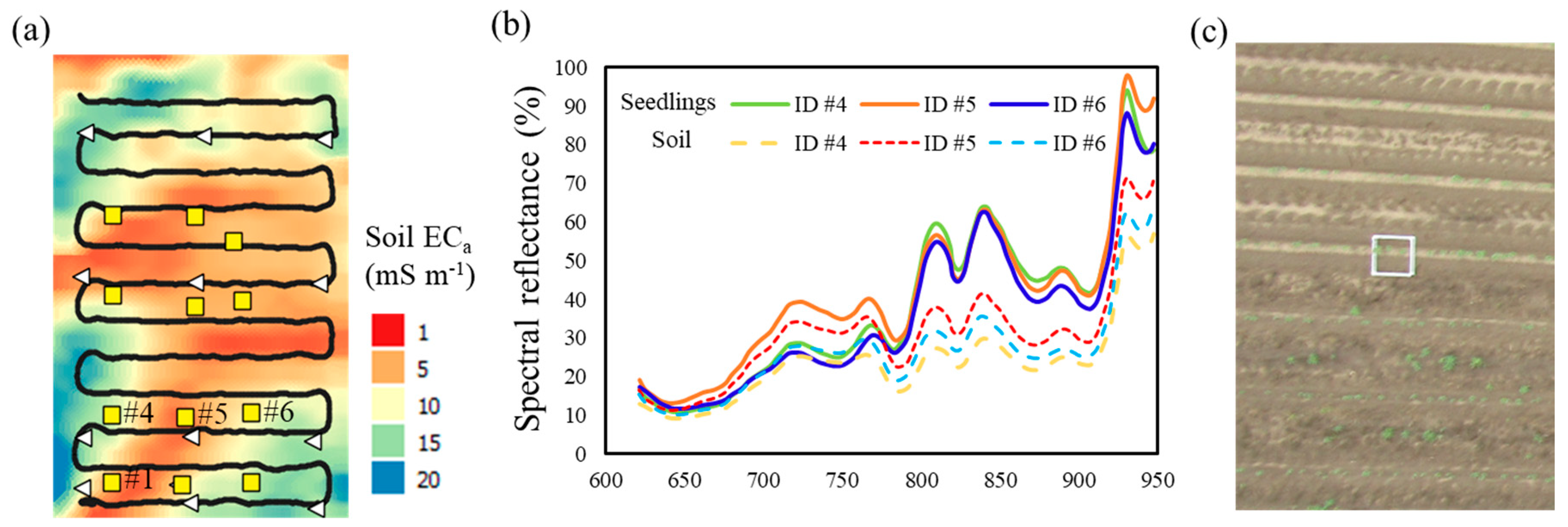
2.1. Experimental Field and Ground Data Collection

This study was conducted in a cotton research field at the Fisher Delta Research Center of the University of Missouri, located in the upper portion of the Mississippi River Delta region near Portageville, MO, USA (36.411° N, 89.697° W). The experimental field has dimensions of about 320 m × 160 m with the long dimension in the south-north direction. The spatial variability of soil texture in the field is large due to both alluvial and seismic activities. Soil texture is closely related to water holding capacity, which may significantly affect plant emergence and production [36]. Apparent soil electrical conductivity (EC_a), a good indicator of soil texture [37], was mapped using a Veris 3100 instrument (Veris Technologies, Salina, KS, USA) equipped with a GPS system in 9 May 2016.

Cotton cultivar PHY 375 WRF (Dow Agrosciences, Indianapolis, IN, USA) was planted on bedded soil using a commercial planter (John Deere 1700, Moline, IL, USA) on 16 May 2018, at a seeding rate of 12 seed/m in a south-north direction with a row spacing of 0.97 m, resulting in 148 crop rows in total. There was no irrigation applied from planting to the date of image data collection.

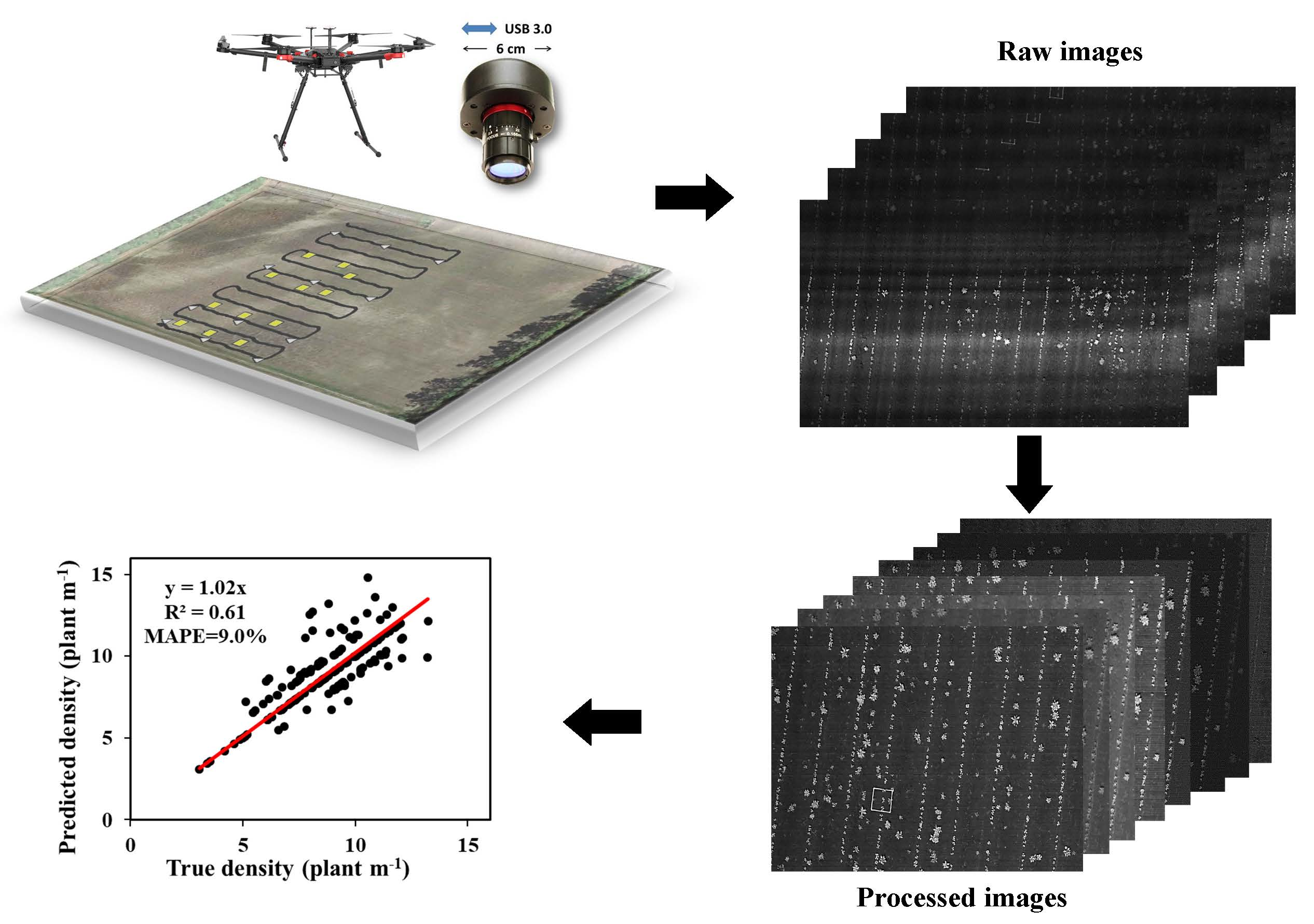
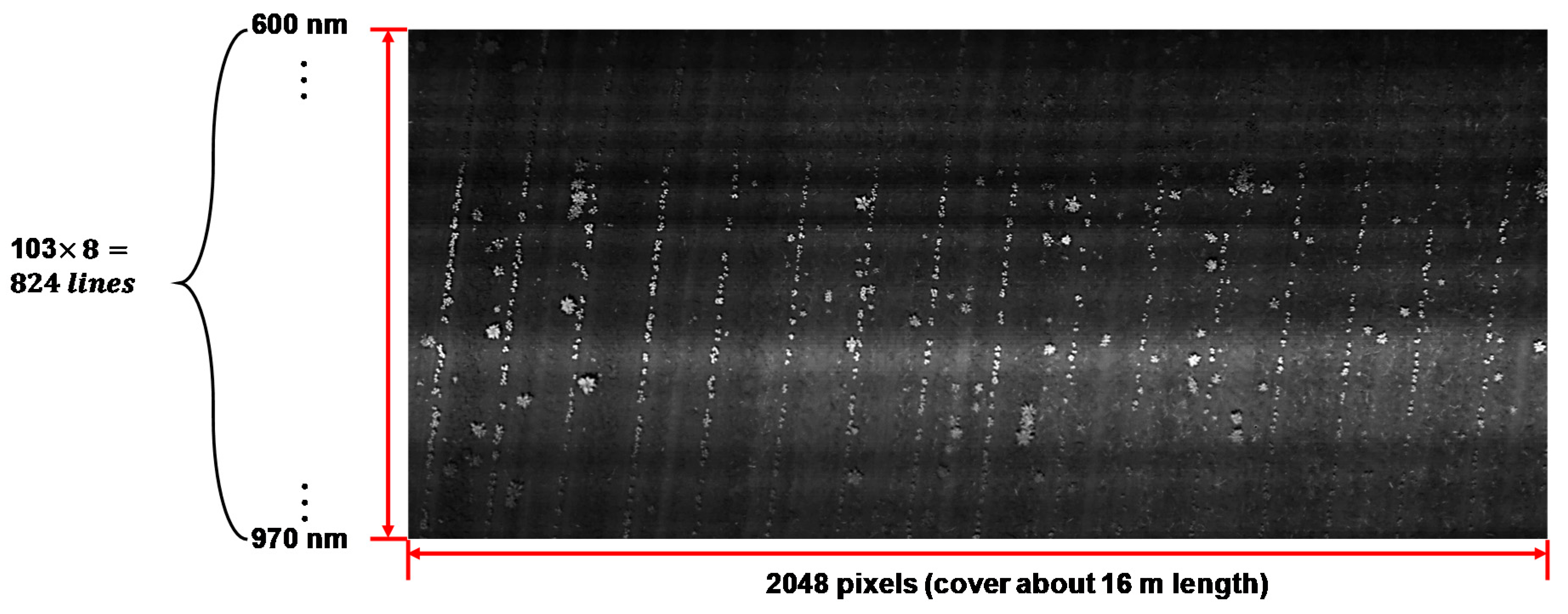
2.2. UAV Imagery Data Acquisition

Imagery data were collected using a UAV-based hyperspectral imaging system consisting of a UAV platform (DJI Matrice 600 Pro, DJI, Shenzhen, China) and a pushbroom hyperspectral camera (OCI-UAV-1000, BaySpec Inc., San Jose, CA, USA). A UAV control app (Autopilot, Hangar Technology, Austin, TX, USA) was used to plan flight paths and set way-points, flight speed, and height. Before flying, flight speed (5.5 km/h) and height (50 m AGL) were planned to achieve a high image overlap (99.3% in the forward direction in this study) required for stitching images. Images were only collected for the center part of the field (Figure 1) due to the 20-min flight limitation of the UAV batteries available at the time. The hyperspectral camera included 103 spectral bands with a bandwidth of 2–5 nm in the spectral range of 600–970 nm. A tablet computer (Surface Pro, Microsoft, Redmond, WA, USA) mounted on the UAV platform was used to control the camera and collect data using the camera control software (SpecGrabber, Bayspec Inc., San Jose, CA, USA). The GSD was 0.79 cm/pixel at the flight height of 50 m AGL with a frame size of 1088 × 2048. Before taking off, the exposure time was set properly to avoid overexposure. A white poster board, whose reflectance from 350 nm to 1000 was measured using a spectrometer (Jaz, Ocean Optics Inc., Largo, FL, USA), was used for white radiometric calibration. The initial frame rate of the camera was set as 35 frames per second (fps); however, the frame rate was reduced on occasion due to overheating of the tablet. The collected images were saved on the solid-state storage hard drive (SSD) of the tablet and were downloaded for further processing after flying. Ground reference points (GRPs) consisting of 12 fence posts (~1.1 m above ground) with white polytechnic boards (30 cm × 30 cm) and twelve 53 cm × 53 cm squares constructed with half-inch polyvinyl chloride (PVC) pipes were distributed throughout the field for GSD calibration after image alignment and stitching. Figure 1 shows the positions of the GRPs (squares in the image). Image data were collected near solar noon (around 12:50 p.m. Central Daylight Time) at 15 days after planting on 1 June 2018. Weather was stable and considered constant during data collection.

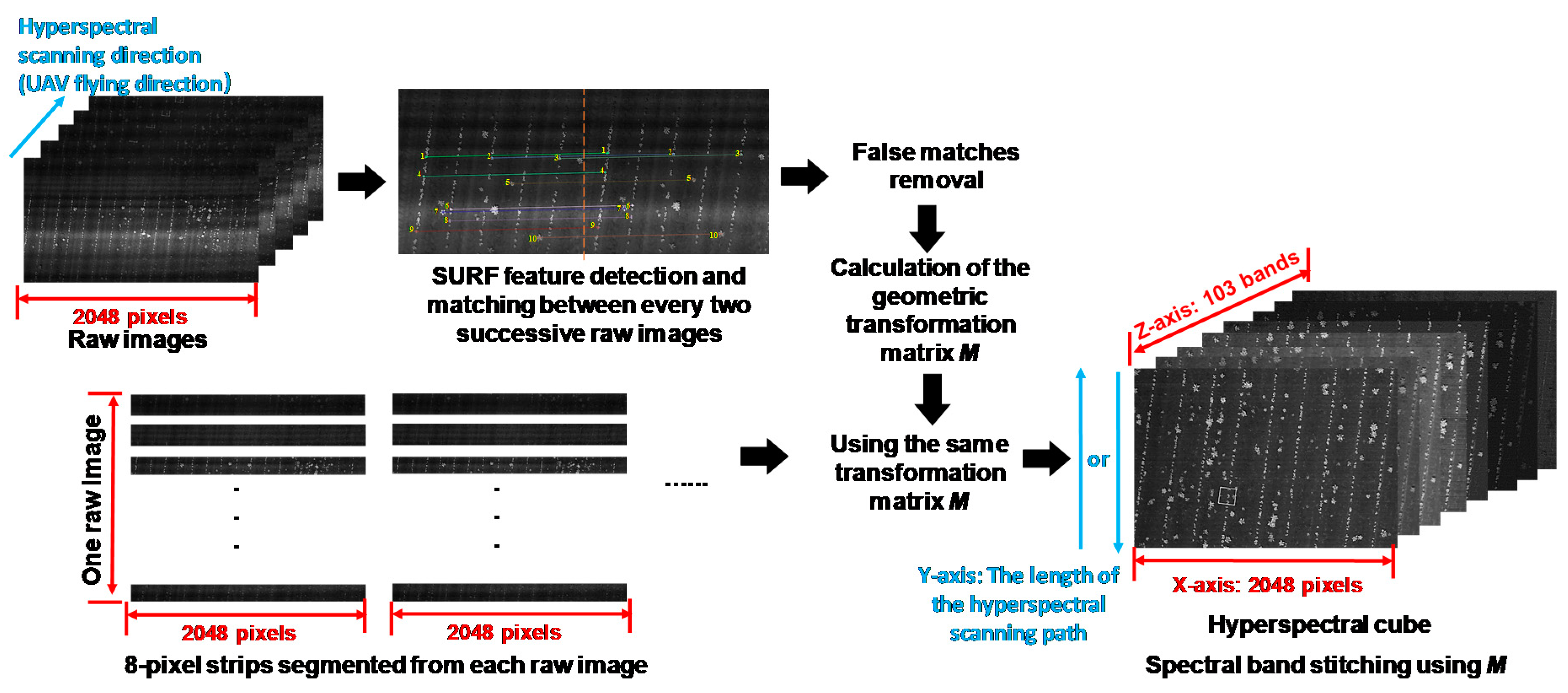
2.3. Image Alignment and Stitching

An image frame, referred to as a raw image henceforward, collected by the pushbroom hyperspectral camera was an 8-bit grey scale image. One raw image collected in the test field (Figure 2) shows that each image frame includes 824 × 2048 effective pixels. The 824 pixels in the vertical direction are generated by the 103 bands of the camera, with eight pixels per band, i.e., 103 × 8 = 824 pixels. There are 2048 pixels for each spectral band forming a so-called spectral line in the horizontal direction, which covered 16 m on the ground when acquired at 50 m AGL.

The UAV-based imaging system scanned the field along the UAV flight direction as shown by the blue arrows in Figure 1. To generate a panorama of the target field in each spectral band, an algorithm was developed to process the raw images. This was required due to low accuracy in alignment and stitching when using the CubeCreator software supplied by the camera manufacturer (BaySpec Inc., San Jose, CA, USA). The processing procedure included (1) feature detection and matching, (2) removal of false matches, (3) calculation of a geometric transformation matrix, and (4) development of spectral band stitching images. The workflow of the stitching process is illustrated in Figure 3. Raw image features were detected to stitch the successive images. Then, the matching features between every two successive raw images were used to calculate a transformation matrix M. Each raw image consisted of 103 bands, each 8 pixels wide (as described in Figure 2). To generate a panorama image for each band, the 8-pixel strips of each band were segmented from all the raw images, and stitched using the same transformation matrix M calculated from the raw image frames. In the end, spectral cubes containing 103 bands in the Z-axis (Figure 3) were generated. These cubes had the same 2048-pixel width as the raw images in the X-axis, and the Y-axis corresponding with the length of the image scanning paths of the two scanning directions (see Figure 1). The final spectral cubes were the panorama images collected for each UAV flight path.

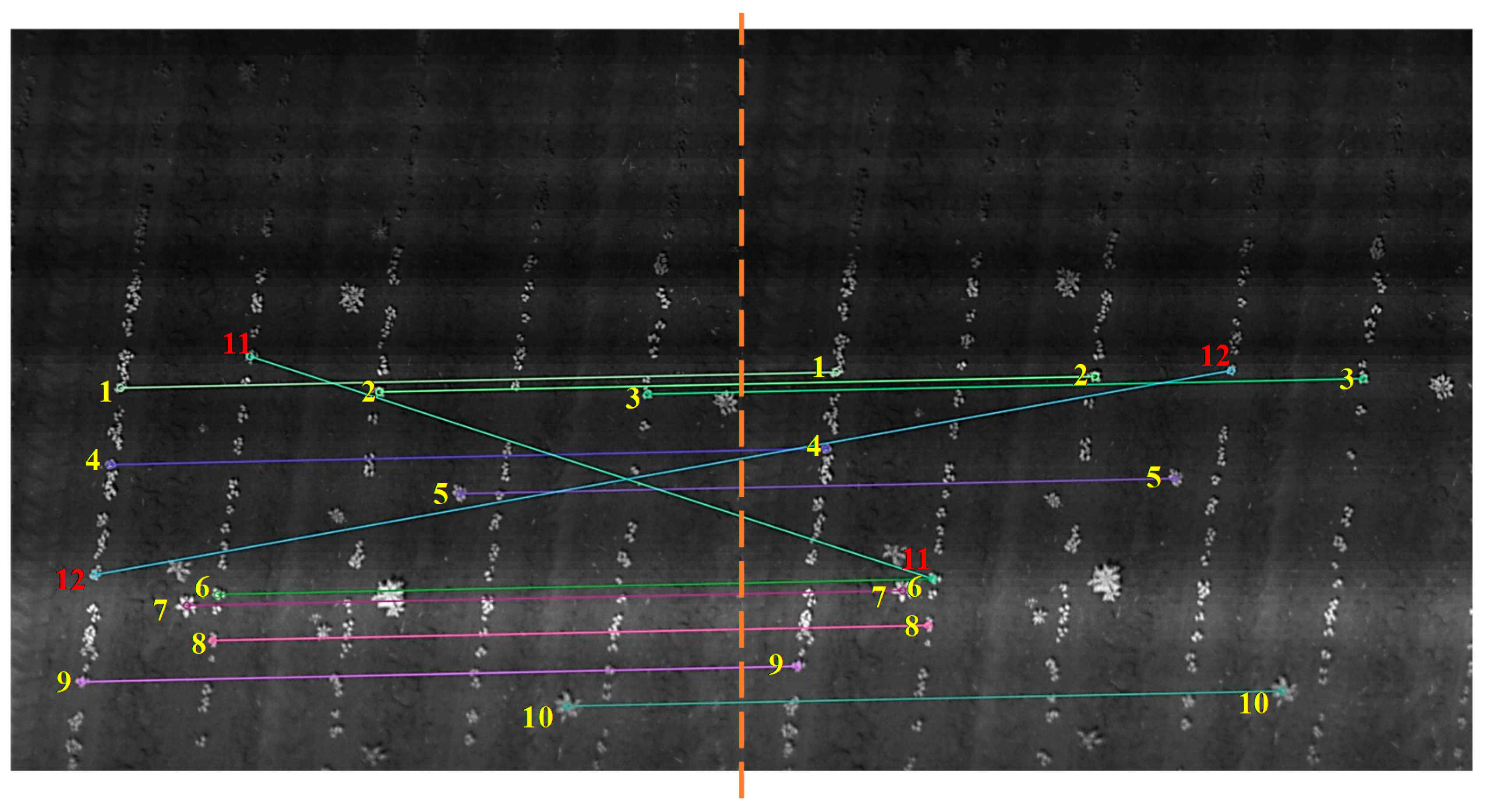
2.3.1. Feature Detection and Matching

Image features were detected using the method of Speeded-Up Robust Features (SURF), a 128-dimension (8 orientation bins for each of the 4 × 4 location bins) local feature detector and descriptor developed in [38]. As a scale-invariant feature, SURF used image pyramids and different sized box filters to find points of interest at different scale spaces [39]. The scale space of SURF was divided into octaves and each octave was subdivided into a constant number of scale levels. The number of pyramid octaves and of octave layers were both set to 4 in this study. After feature detection, the k-nearest neighbors (KNN) algorithm was used to match the most similar feature pairs in two successive raw images. The KNN calculated all of the Euclidean distances of features with each other to find the closest K matches. In this study, K was set to two (K = 2); therefore, the KNN algorithm returned the two closest key points for each key point to be matched.

2.3.2. Removal of False Matches

False matches were those pixels that had the shortest Euclidean distance but were different objects in the successive images. To detect and remove false matches, a distance ratio test was conducted to compare the Euclidean distance of the closest key point to that of the second-closest key point identified by KNN [39]. It was assumed that the first closest key point came from the same object as the key point to be matched, while the second-closest key point came from another object. Distance ratio tests checked the similarity of the two nearest matches to select the matches with high similarity in successive images that were not reliable and should be removed. All matches whose distance ratio test was greater than 0.75 were removed in this study.

The images were collected on a calm day, and the UAV was parallel flying with the ground with minimum variations in roll and pitch, but small adjustments in yaw angle due to navigation error (flight heading, speed and height). Therefore, the geometric transformations for matching any two successive images only included the operations of translation, scale and rotation. Considering the low flight speed of the UAV and the high degree of image overlap, the rotation and scale factor of two successive images were less than 0.03 degrees and 0.005 based on statistical analysis of 20,000 matches obtained in this study. Therefore, in the case where scale and rotation were small enough to be negligible, the matching lines of the correct matches should have similar slopes and lengths. The slope and length of the matching lines were calculated using Equations (1) and (2):

$$slope=\frac{y_2-y_1}{x_2-x_1}$$

(1)

$$length=\sqrt{{\left(x_2-x_1\right)}^2+{\left(y_2-y_1\right)}^2}$$

(2)

where, (x₁, y₁) and (x₂, y₂) are the coordinates of a key point and its matching point in two successive images. The matches were considered to be false matches if the slopes and lengths of the matching lines had a large difference from other matches, as for the two red matches in Figure 4. Thresholds of 0.15 degrees for slope and 30 pixels for length were used for determining false matches.

Another way to determine false matches was to calculate the ratio of the slope and the length of one matching line to the mean value of all matching lines in two successive images. The ratios of the slope and length of the correct matches would be close to 1. The thresholds for false matches were set as lower than 0.9 and greater than 1.1. Both the methods discussed above were used in this study to remove false matches.

2.3.3. Calculation of the Geometric Transformation Matrix

Once the correct matches were identified, transformation matrices of each pair of two successive images were calculated. As mentioned earlier, only translation, scale and rotation were considered in this study. The transform matrix M is shown as Equation (3) [40]:

$$M=\left[\begin{array}{ccc}{s}_x·cos\theta & -sin\theta & t_x\\ sin\theta & s_y·cos\theta & t_y\end{array}\right]$$

(3)

where, t_x and t_y are the distance in pixels of translation in the horizontal and vertical directions, s_x and s_y are the scale factors in the horizontal and vertical directions, and θ is the rotation angle. Assuming a pixel value of an image coordinate I(x, y) was to be transformed into its previous image coordinate I’(x’,y’), Equation (4) shows the transformation of these two images based on the transform matrix M:

$$M=\left[\begin{array}{ccc}{s}_x·cos\theta & -sin\theta & t_x\\ sin\theta & s_y·cos\theta & t_y\end{array}\right]$$

(4)

where, (x, y) and (x’, y’) are image coordinates of image I(x, y) and I’(x’,y’). The initial values of t_x and t_y were the mean distance of all matches in two successive images, the initial value of θ was set as 0 degrees (no rotation), and both scale factors, s_x and s_y were set to 1 (no scaling). A grid search iteration method was used to search for the optimum solutions of the five parameters in M [41]. Due to the small changes between the two successive images in this study, the search ranges of translation distance were set as ±10 pixels with an increment of 0.2 pixels, the scale factor was 0.9995 to 1.0005 with an increment of 0.00025, and the rotation range was –0.065 to 0.065 degrees with an increment of 0.005 degrees. A corresponding image $I^{\prime }\left(\widehat{x^{\prime }},\widehat{y^{\prime }}\right)$ would be generated based on each search result and I(x, y). The error was defined as the sum of Euclidean distances between I’(x’,y’) and $I^{\prime }\left(\widehat{x^{\prime }},\widehat{y^{\prime }}\right)$, shown as Equation (5):

$$error={\displaystyle \sum }_{i=0}^n\sqrt{{\left({{\mathrm{x}}^{\prime }}_i-{\widehat{{\mathrm{x}}^{\prime }}}_i\right)}^2+{\left({y^{\prime }}_i-{\widehat{y\prime }}_i\right)}^2}$$

(5)

where, n is the number of matches in both I’(x’,y’) and $I^{\prime }\left(\widehat{x^{\prime }},\widehat{y^{\prime }}\right)$.

2.3.4. Dynamic Panorama and Spectral Band Stitching

There were two main steps within the stitching algorithm (see Figure 3): (1) the raw images were used to calculate M; (2) M was used to stitch every 8-pixel spectral band strip of the raw images to generate 103 spectral band panoramas. The reason that M had to be calculated using raw images is that it was impossible to get enough feature matching using only 8-pixel spectral band strips.

When calculating each M using every two successive raw images, each raw image was added to the panorama based on Equation (4) one at a time, aligning the raw image with the previous raw images already in the panorama. The panorama expanded its original boundary dynamically according to the coordinates of the four corners of each new added raw image.

The panorama developed in this study combined approximately 2200 raw images in each flight path. It was inefficient to perform SURF feature detection on the entire panorama every time a new raw image was added. Therefore, the SURF feature detection was only conducted in one previously added raw image. With each raw image added to the panorama, the coordinates of its four corners on the panorama were recorded. The SURF feature detection was only conducted on the region bounded by these four corners instead of the entire panorama. Once the feature detection was done in this raw image, it was used for matching with the next raw image and calculating the next M for the next raw image stitching. M of every two successive images was recorded in a txt file.

When the txt file that included all the M values for every two successive raw images had been established, it was used for panorama stitching of each spectral band. A panorama of each spectral band was generated by the 8-pixel spectral strips segmented from raw images. To apply the transformation matrix M calculated from the raw images, the same image size was required instead of the 8-pixel image height of the spectral strips. Therefore, each 8-pixel spectral strip was padded with zeros to the same size as the raw image and this image was used for the spectral band panorama stitching. Only non-zero-pixel values were added to the spectral band panorama one at a time using Equation (4).

2.3.5. Alignment Error in Images of Different Bands

Ideally, images of the 103 spectral bands are aligned pixel by pixel. However, there is always error in alignment due to camera movement, sequential sensing of the 103 channels, and issues with the algorithms used to conduct the alignment [42]. To evaluate the alignment accuracy of images in all 103 bands, an indicator of alignment error was defined as the average coordinate shift (mean of Euclidean distances between image pixels) of the same objects in each two different spectral bands. In this study, the GRPs that were clearly identified were used as reference objects to test the alignment performance. We manually recorded the coordinates of the four corners of the square PVC pipes in 103 spectral panoramas and calculated the shift. The raw images collected in the first flight path that contained three PVC pipes were stitched using the commercial CubeCreator software associated with the hyperspectral camera and the algorithm of this paper to compare their alignment errors. All processing of the stitching algorithm in this section was conducted using the Opencv v3.4.2.16 package in Python [43].

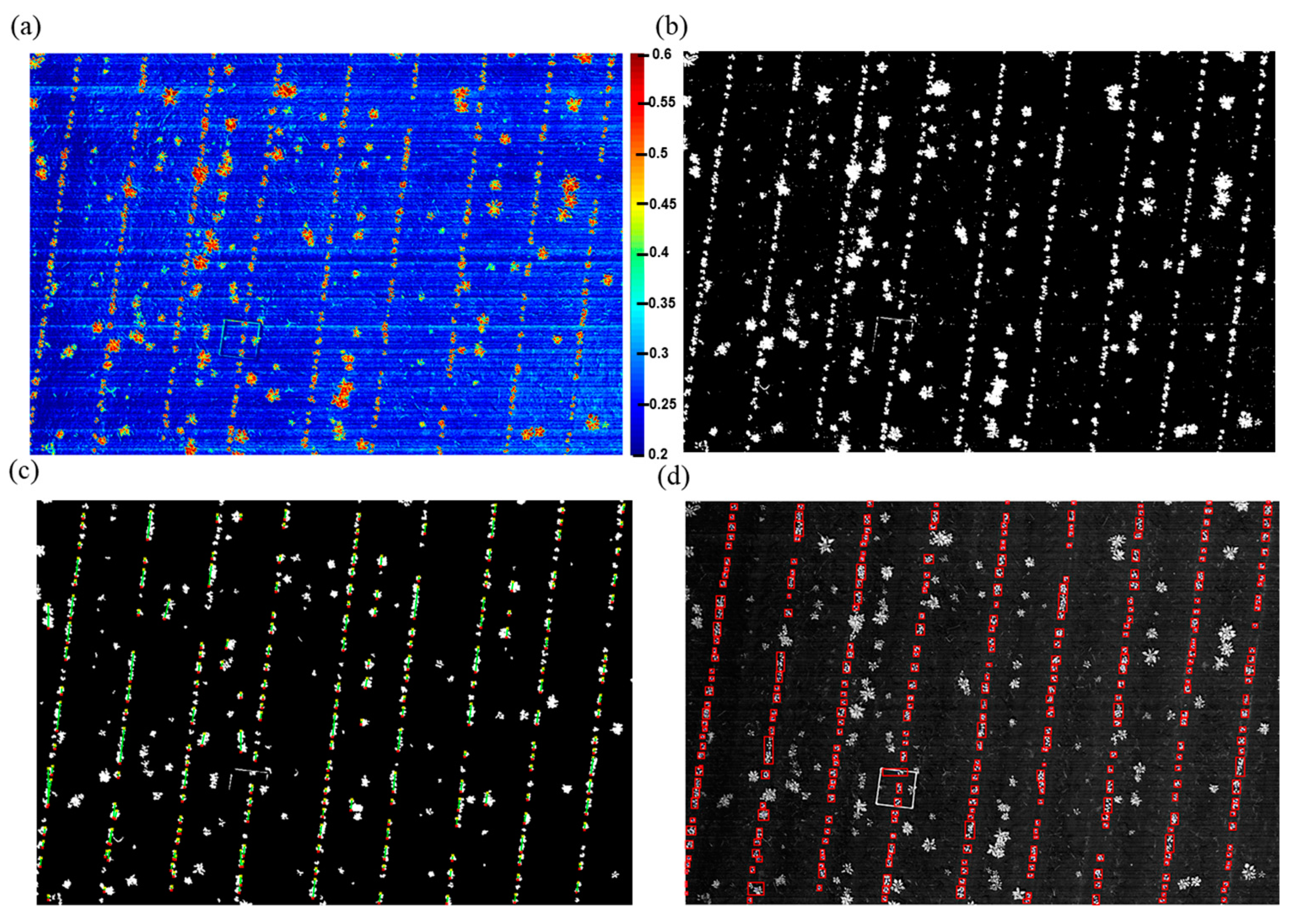
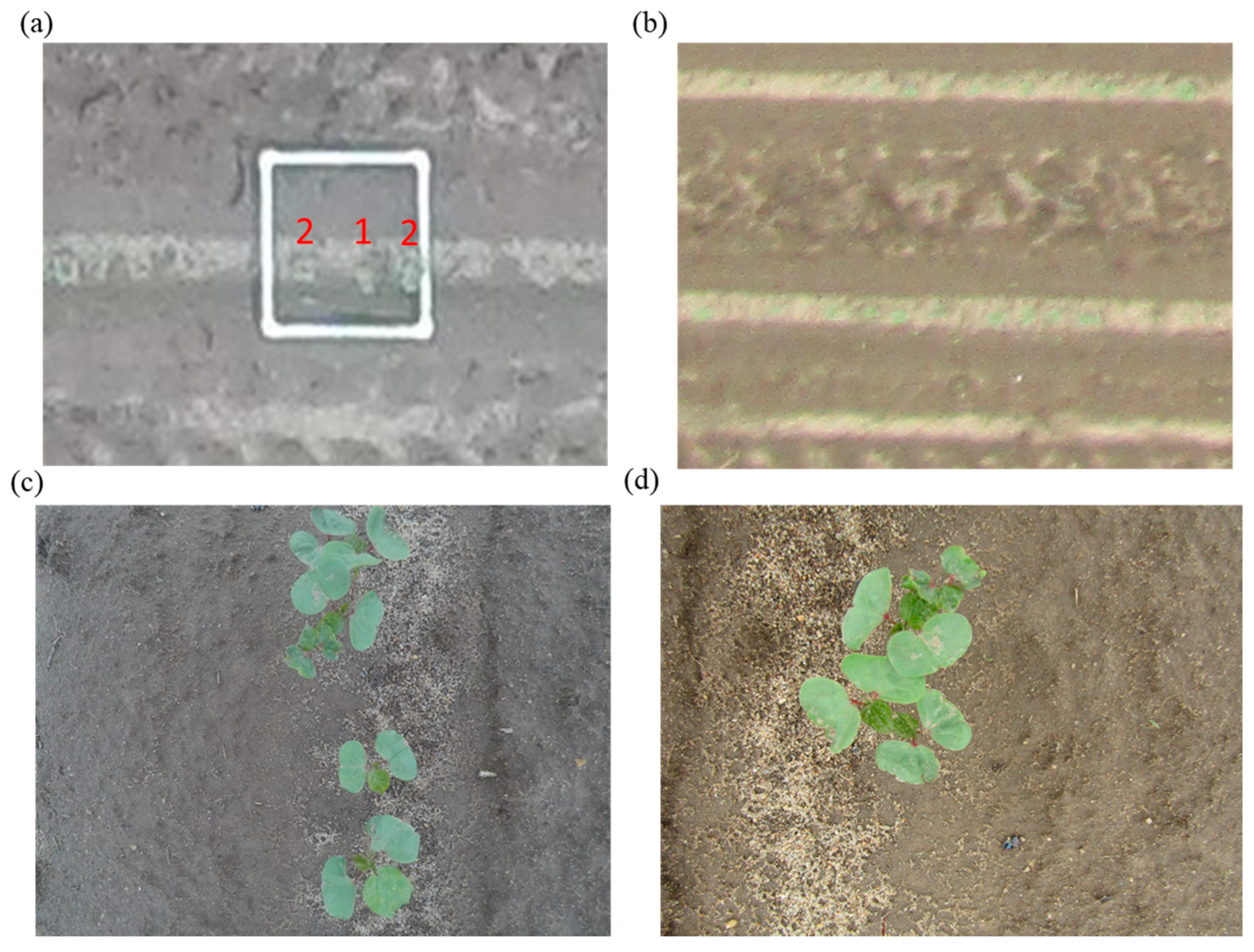
2.4. Segmentation of Cotton Stand

Two previous studies [44,45] summarized the widely used narrow-band spectral reflectance indices for various applications in different crops, including NDVI, fluorescence ratio index, and water normalized difference vegetation index. In this study, several spectral reflectance indices, including four NDVI and two normalized difference red edge (NDRE) indices calculated with different bands were examined for identifying suitable indices for seedling segmentation. To segment plants from images, it is desired to have large difference between vegetation indices of plants and soil. Figure 5 shows the histograms of three vegetation indices that have different ability to distinguish plants and soil.

Image histograms and visual observations confirmed that NDVI calculated using Equation (6) gave the largest contrast between cotton seedlings and soil:

$$NDVI=\frac{R_{841}-R_{667}}{R_{841}+R_{667}}$$

(6)

where, R₈₄₁ and R₆₆₇ are the pixel values in the images of 841 nm and 667 nm bands. Figure 6a shows that the NDVI values of soil and non-soil (crops and weeds) had sufficient contrast to remove soil with a threshold of NDVI <0.35. The threshold may need to be changed for other studies according to the soil texture and crop conditions. Figure 6b shows the binary image after soil was removed where the connected regions might be cotton seedlings, weeds and/or noise. The small objects, including most of the noise, were removed using a connected region threshold of <20 pixels. Meanwhile, the connected regions >350 pixels were considered to be weeds and were removed (Figure 6c). To segment cotton crop rows, a Standard Hough Transform (SHT) [46] was applied to search the long lines in the images. Weeds growing in inter-rows were inconsistent and had fewer pixels compared to crop rows. Therefore, the false SHT-detected lines due to weeds were removed by detecting the lines with less than 10 objects. After the crop lines were identified, the Euclidean distances between the center of each connected region and the lines were calculated, and the objects that had a distance of less than eight pixels from a crop line were assigned to the closest objects (seedling or seedling cluster) in this row while the rest were considered to be weeds in inter-rows. After the above pre-processing, each of the remaining objects was defined as one region of interest (ROI) (i.e., the object in each red box in Figure 6d). One ROI might contain one single seedling or multiple connected seedlings as a cluster. All the image processing procedures described in this section were conducted in Matlab R2018a (MathWorks, Inc., Natick, MA, USA).

2.5. Evaluation of Cotton Stand Count

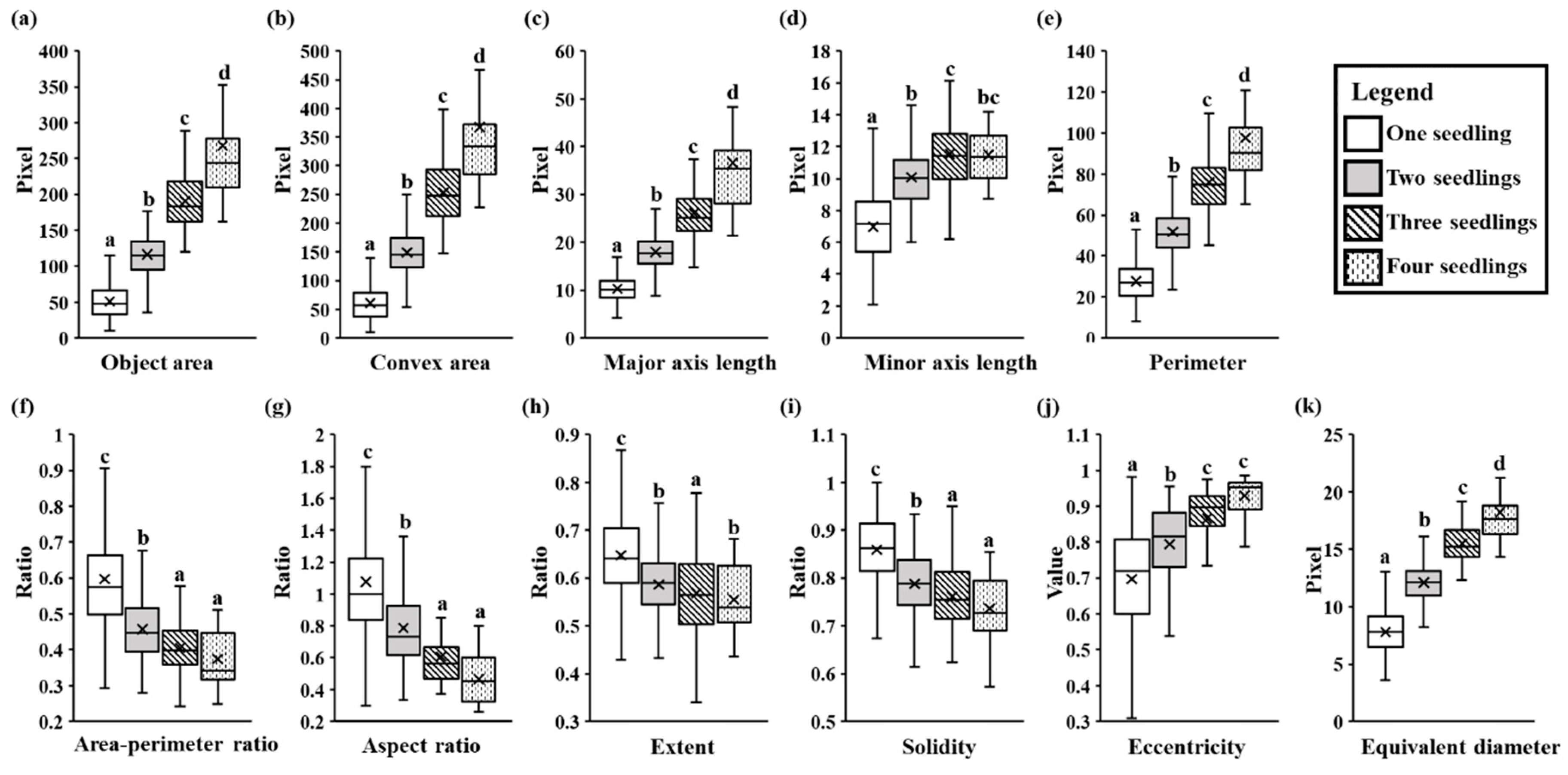
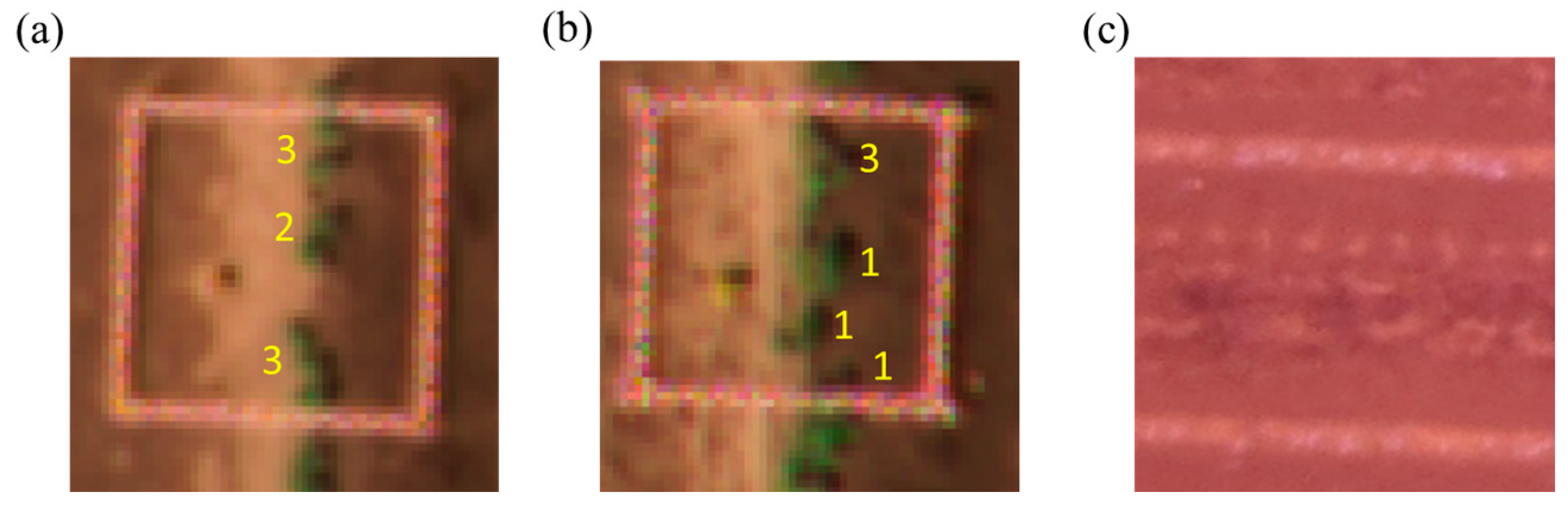
2.5.1. Image Features for Determining Number of Seedlings

Crop stand is generally quantified as the number of plants per a fixed length of crop row or a fixed unit of field area [8,11]. To obtain an accurate stand count, it is important to count the number of single plants that clustered in a ROI. Eleven morphological features [47], including shape, dimension and pattern, were defined to differentiate each ROI with multiple seedlings, as shown in

Table 2. Image features used to segment individual cotton seedlings.

Feature	Name	Definition
F1	Object area	The total number of pixels of the objects in a ROI
F2	Convex area	Area (number of pixels) of the smallest convex polygon of a ROI
F3	Major axis length	Length (in pixels) of the major axis of the ellipse in a ROI
F4	Minor axis length	Length (in pixels) of the minor axis of the ellipse in a ROI
F5	Perimeter	The perimeter (in pixels) of a ROI
F6	Area-perimeter ratio	The ratio of object area within ROI to its perimeter
F7	Aspect ratio	The ratio of width to height of the bounding box of a ROI
F8	Extent	Ratio of object area to the pixels of the bounding box
F9	Solidity	Ratio of the object area to convex area
F10	Eccentricity	Eccentricity of the ellipse that has the same second-moment as the ROI
F11	Equivalent diameter	Diameter of a circle with the same area as the ROI

.

Analysis of variance (ANOVA) was used to compare the values of the 11 features for different numbers of seedlings (i.e., one, two, three, or four) in an ROI at a significance level of 0.05 based on Tukey’s Honest significant difference test. The goal of this analysis was to determine if these features could accurately distinguish the number of seedlings in each ROI. Since feature pairs (or groups) with a strong linear relationship were considered to be redundant variables [48], Pearson correlation coefficients between each two of these features were calculated and principal component analysis (PCA) [49] was used to replace those features with strong linear relationships with fewer linearly uncorrelated variables. Variables without collinearity and PCA-derived variables were combined in a new data set for further use. The above statistical analyses were conducted using R software (RStudio Desktop 1.1.453, RStudio, Boston, MA, USA).

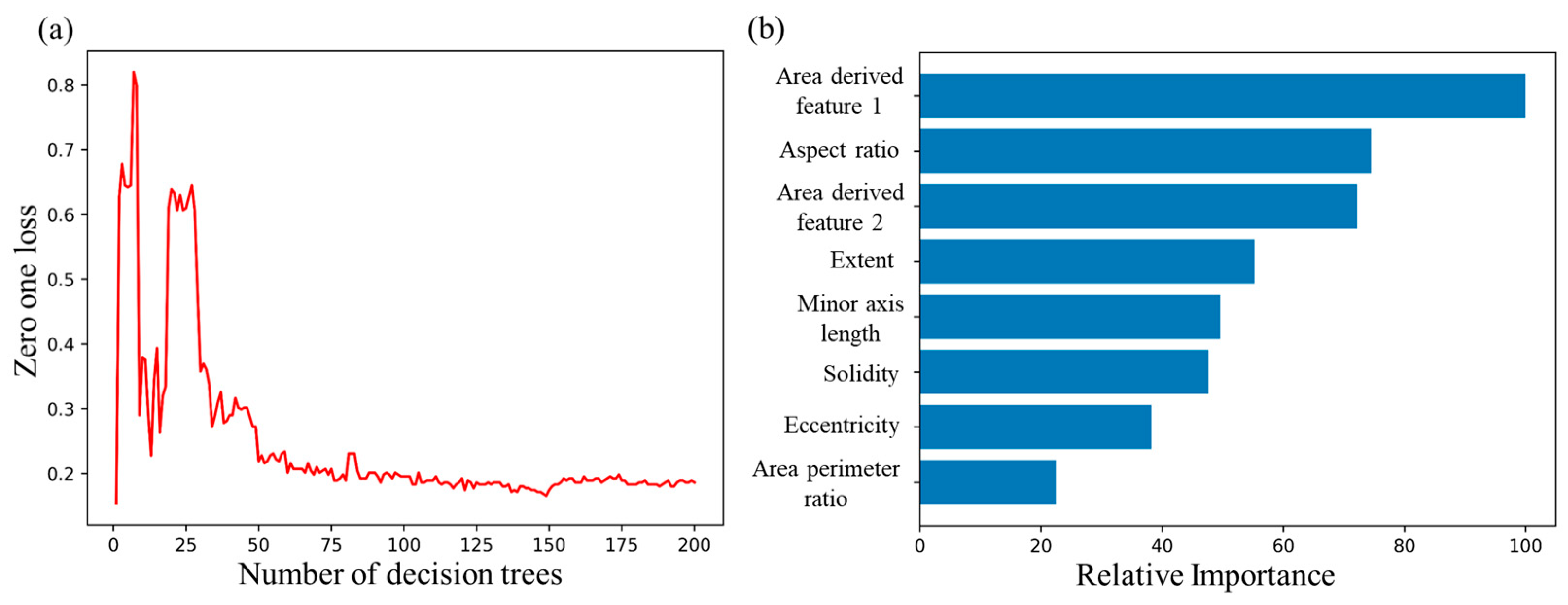
2.5.2. Development of Decision Tree Model

A decision tree classifier was used to identify the number of cotton seedlings in each ROI using the new combined data set. To establish the training and testing dataset for the decision tree model, a total of 1200 ROIs were identified using the procedure in Section 2.4 from three sections of different flight paths, and the number of seedlings in each ROI was manually counted and labelled. Before counting, a series of image pre-processing methods, including gamma correction, Laplace enhancement and contrast adjustment, were used to improve the clarity of the images to make visual counting easier. The features of the 1200 ROIs and their corresponding labels were split into two sets: 70% as the training set, and 30% as the testing set. A decision tree model is not robust with a small number of tree branches, but the model might over fit when too many branches are used [50]. In this study, an ensemble method, AdaBoost [51], that combines many simple decision trees was used to improve the robustness of classification. Decision trees with depth no more than two were used to avoid the overfitting problem. The number of decision trees used in the AdaBoost model was determined by balancing the decision tree number to have sufficient classification accuracy and lower overfitting [50]. Therefore, 20% of the training set was used as the validation data set to identify an optimal number of trees using a 5-fold cross-validation. Misclassification error was defined as zero one loss, which assigns 0 to a correct classification but 1 for an incorrect classification [52]. Accuracy was defined as the ratio of the number of correct classifications to the total number in the data set.

The descriptive statistical analysis on the labelled ROIs showed that 76.3% of the ROIs contained one single cotton seedling, 19.3% contained two connected seedlings, 3.8% had three connected seedlings and 0.6% had four connected seedlings. This is an unbalanced data set that might cause errors during the modelling process [53]. Therefore, a naive random over-sampling method was used to generate new samples by random replacement of the minority class(es) to build a balanced synthetic dataset to replace the training set [53].

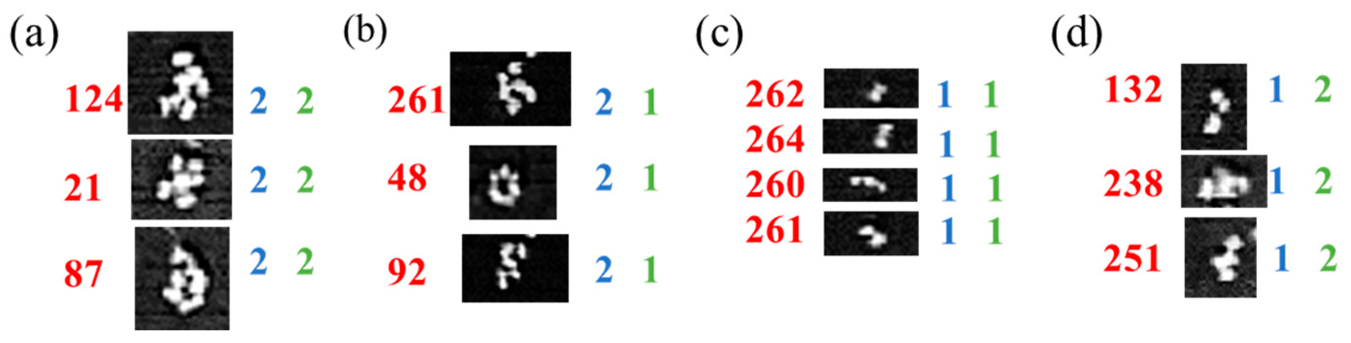
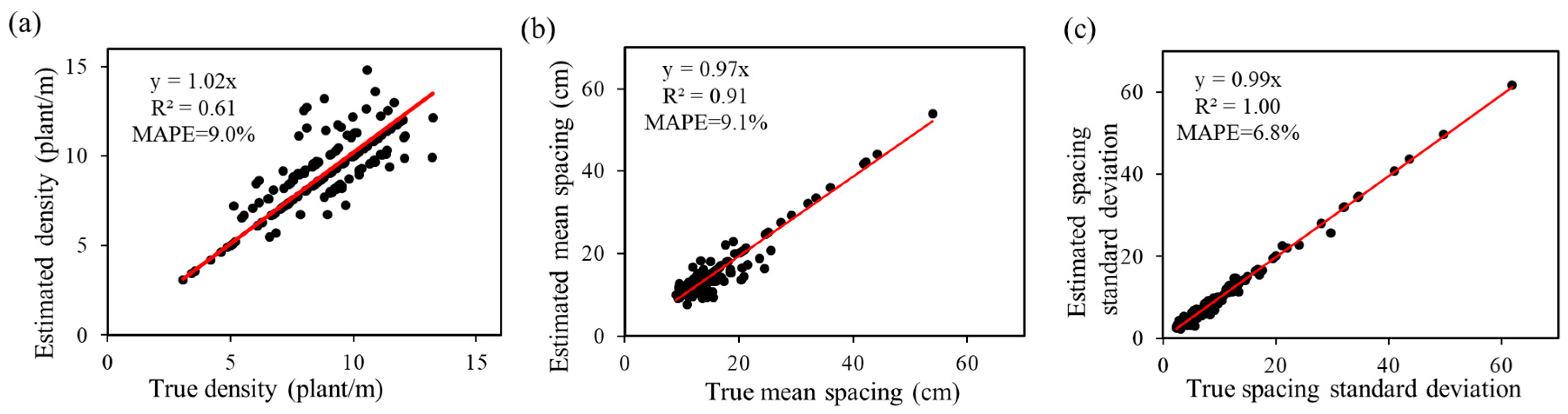
2.5.3. Evaluation of Stand Count and Uniformity

Plant density was defined as plants per meter in a row [6]. In this study we calculated plant density from the total number of cotton seedlings in all ROIs within a 1-m crop row. The GSD was calibrated using PVC pipe squares in flight paths with a dimension of 53 cm × 53 cm. The length of a side of the PVC square averaged 67.8 image pixels, which was 129 pixels per meter in the images (i.e., GSD = 0.778 cm/pixel). The mean spacing ($\overline{x}$) and the standard deviation ($\delta$) of the spacing between plants, shown as Equations (7) and (8) [54], are commonly used for describing seed spacing uniformity [55]. Mean absolute percentage error (MAPE) was used to evaluate the accuracy of the plant density and uniformity estimations:

$$\overline{x}=\frac{1}{n}{{\displaystyle \sum }}_{i=1}^n{x}_i$$

(7)

$$\delta =\sqrt{\frac{1}{n}{{\displaystyle \sum }}_{i=1}^n\left(x_i-\overline{x}\right)}$$

(8)

where, $x_i$ is the seedling spacing (cm) estimated using the imaging method. The seedling spacing was calculated using the distance between the center points of two ROIs containing only single seedlings. If a ROI included m seedlings, the $x_i$ between two neighbor seedlings in this ROI was calculated using Equation (9):

$$x_i=\frac{2L_m}{m}$$

(9)

where, L_m is the major axis length of the ROI. If a seedling is outside a ROI that includes m seedlings, the $x_i$ of the seedling to its neighbor seedling in the ROI was calculated by Equation (10):

$$x_i=D-\frac{L_m}{2m}\left(m-1\right)$$

(10)

where, D is the distance between center points of two ROIs. All processing in this section except for the two statistical analyses were conducted with the Scikit-learn package in Python [56].

3. Results

3.1. Alignment Error

Table 3. Comparison of the alignment error (pixels) using both CubeCreator and the algorithm developed in this study.

Sample Points	1	2	3	4	5	6	7	8	9	10	Average/std
CubeCreator	164.0	165.0	165.0	165.7	185.4	186.0	187.1	197.6	198.0	197.2	181.1 ± 13.9
This study	3.6	3.2	2.9	3.5	2.6	2.3	2.4	2.6	2.7	2.6	2.8 ± 0.4

shows the alignment error in pixels of shift using algorithms from CubeCreator and the one developed in this study. It can be seen from the table that the alignment errors of the 10 samples processed by the CubeCreator were substantially larger than those obtained from the algorithm developed in this study. The results indicate that the image alignment and stitching method proposed in this study provided an effective way to process data from the pushbroom imaging system.

3.2. ROI Feature Analysis

Mean values of all features defined in Table 2 for ROIs with different numbers of cotton seedlings were found to be significantly different (Figure 7). The object area (F1), convex area (F2), major axis length (F3), perimeter (F5) and equivalent diameter (F11) in the ROIs with more seedlings were significantly greater than those with fewer cotton seedlings (Figure 7a–e,k). Since cotton was planted in rows, if seedling number increased in a ROI, this tended to increase the major axis length (F3) to a greater extent than the minor axis length (F4). (Figure 7c,d). For the same reason, aspect ratio decreased when the number of cotton seedlings increased (Figure 7g). When image data were collected, cotton seedlings showed two different growth stages, whereby some had only two cotyledons, while others had two cotyledons and one true leaf [57], which might be caused by the variation of soil conditions, seed vigor and planting depth. The single cotton seedlings showed different sizes and shapes in the images. If a ROI only included one cotton seedling, eccentricity (F10) could have a large variance due to the differences in seedling shape. ROIs with more cotton seedlings were longer than those with fewer seedlings, and the eccentricity would become close to 1, while the variance decreased (Figure 7j). These results show that the features extracted in this study could effectively distinguish ROIs with different numbers of cotton seedlings.

Table 4. Correlation matrix between features. Features with * are highly correlated (r > 0.9).

Feature	F1	F2	F3	F4	F5	F6	F7	F8	F9	F10	F11
F1 *	1.00
F2 *	0.99§	1.00
F3 *	0.94	0.97	1.00
F4	0.78	0.75	0.62	1.00
F5 *	0.94	0.97	0.97	0.75	1.00
F6	0.30	0.29	0.29	0.21	0.28	1.00
F7	–0.53	–0.53	–0.54	–0.48	–0.56	–0.17	1.00
F8	–0.37	–0.43	–0.47	–0.37	–0.52	–0.11	0.27	1.00
F9	–0.47	–0.56	–0.62	–0.47	–0.69	–0.16	0.41	0.78	1.00
F10	0.35	0.39	0.53	–0.08	0.41	0.24	–0.22	–0.29	–0.37	1.00
F11 *	0.97	0.95	0.91	0.87	0.94	0.30	–0.58	–0.41	–0.53	0.32	1.00

§: bold numbers mark the numbers of r > 0.9.

shows the correlation matrix between each pair of features, which shows that the Pearson correlation coefficients among F1, F2, F3, F5 and F11 were greater than 0.9 because they were all area-derived features. These five features were normalized to the range of [0, 1] and used as for a PCA analysis to generate two area-derived features to replace the highly correlated features. After conversion, the new data set consisted of eight features.

3.3. Evaluation of Cotton Emergence

The new data set was used to develop a classification model based on the AdaBoost model for the evaluation of cotton stand count. The variation of zero one loss of models with different numbers of decision trees calculated using the validation data set is shown in Figure 8a, indicating that the classification errors were unstable [48] when the number of decision trees was less than 35. As the number of decision trees increased, the classification error decreased and became more stable. The model obtained the lowest error rate when the number of decision trees was 150 but increased slightly afterward, which might be due to over-fitting. Therefore, the number of decision trees was set at 150.

The relative importance of the eight features, which indicates that the two area-derived features and aspect ratio were the most important parameters for estimation of the number of cotton seedlings in each ROI is shown in Figure 8b. These results are consistent with those from other published papers. For example, the area feature was the most commonly used feature for crop counting in early growth stages as found by [9]. Object orientation and extent were the most important features for counting crops with slender leaves such as wheat as shown by [6], while length-width ratio, density and border length were more important for counting crops with round leaves such as rapeseed as highlighted by [11].

The manual count of cotton seedlings of the 360 ROIs in the test data set was 501, and the estimated number was 491, or 2% less than the manual count, indicating good performance in estimating the overall stand count. The accuracy for classifying the ROIs with different number of seedlings in the test dataset using the developed method was 84.1%. Figure 9 shows the confusion matrix including the number of ROIs classified in each category and their percent (e.g., percent of classified ROIs in category of one seedling is 181/[181 + 17 + 1] × 100 = 91%).

It can be seen that most of the misclassifications happened in ROIs containing two and three seedlings, which were fewer in number compared to those with one seedling. The low classification accuracy in such categories reduced the overall classification accuracy. The possible reasons for misclassification are many, but the main reason may be the large variation in seedling size, shape and the ways of leaves overlapped. The variation in seedling may due to the various characteristics of the seedbed (variation in soil moisture, soil texture, organic matter, surface residues, and soil temperature), planting equipment (variation in planting depth and seed distribution), and seed quality [58]. Figure 10 shows some examples of seedlings with different size, shape and overlap. Figure 10a,c show that number of seedlings in all three ROIs was classified correctly. However, the number was misclassified in the ROIs in Figure 10b,d due to the various sizes of seedlings that confused the algorithm. Although all the ROIs in Figure 10c,d included one seedling, they have different area sizes and shapes, which might be caused by different growth rates due to different soil conditions. All ROIs in Figure 10a,b included two cotton seedlings but they show different overlapping shapes. Combining these data with soil data to establish a spatial correlation model is an area of future study.

The density and uniformity of the cotton seedlings in the 1200 ROIs were calculated to evaluate the performance of the developed models. Figure 11 shows the fit between the manual count (true values) and the estimated number of seedlings in all ROIs. It can be seen that the estimated density and uniformity are highly correlated with the manual measured values with limited errors (MAPE = 9.0%, 9.1% and 6.8% for density, mean seedling spacing and standard deviation, respectively). All data points were close to the 1:1 line indicating a good fit between true values and estimated values. To explore the potential reason for the errors, Figure 12 shows three examples of mean spacing and standard deviation. In Figure 12a, the seedling spacing was uniform but some of them overlapped, which resulted in a smaller mean seedling spacing than that of Figure 12c, where the cotton seedlings had uniform spacing and no overlap. The seedling spacing in Figure 12b was not uniform, leading to a higher standard deviation than that of the seedlings in Figure 12a,c. It can be found from Table 1 that most published studies estimated the stand count at a plot level (18 plots in [11], 6 plots in [9], 90 plots in [8], 40 images in [12] and 30 plots in [19]), which may not provide sufficient site-specific information for precision decision making and further field operations. This study provided a potential approach to estimate the cotton stand at a meter-level scale that has potential to be used in practice.

4. Discussion

The use of narrow-band spectral images in this study addressed inherent problems with RGB and multispectral images for identification of small cotton seedlings. These problems were demonstrated in exploratory research, where two RGB cameras, two multispectral cameras and the pushbroom hyperspectral camera used in this study were compared. Figure 13 shows four frames of RGB images taken using consumer-grade cameras, a GoPro HERO Black 5 (GoPro, San Mateo, CA, USA) and a Canon PowerShot SX410 (Canon INC., Tokyo, Japan), at 15 days after planting in a cotton field. The GoPro camera had a resolution of 12 M pixels and resulted in GSD of 0.52 cm/pixel at the height of 15 m AGL (Figure 13a), while the image (Figure 13b) from the Canon camera had a GSD of 0.45 cm/pixel. Figure 13c,d are RGB images using the same two cameras at 0.3 m AGL, where the crops were clear and the color of the cotton seedlings was distinguishable from the soil. However, crop color was affected by soil reflectance and was distorted when the proportion of soil in the image was high [20]. Images were also blurred because of the focus issues on the small seedlings [12].

UAV-based multispectral cameras may provide useful spectral information for crop identification, however, their resolution is usually low. We tested a well-calibrated multispectral camera Micasense RedEdge-M for cotton seedling evaluation. The manufacturer recommended that this camera be operated at a minimum of 30 m AGL to reduce the impact of misalignment of the five separate sensors. Figure 14a,b shows two image frames collected at 15 days after planting at an altitude of 30 m AGL, resulting in 2 cm/pixel spatial resolution. However, the PVC pipe squares and cotton seedlings in the images exhibited blurred edges. The limitations of misalignment and spatial resolution in multispectral cameras are challenges to their application in evaluation of cotton seedling emergence.

A customized multispectral camera (XNiteCanonElph130, LDP LLC, Carlstadt, NJ, USA) that was modified by replacing the filter of the green channel of the RGB camera (12 M pixels, Canon Elpp 130, Canon INC., Tokyo, Japan) with a near-infrared filter was tested the same day that hyperspectral images were collected (1 June 2018).

However, half of the images were not focused on the seedling due to the small size of the cotton seedlings, resulting in blurred images, shown as Figure 14c. In addition, the NDVI dynamic range of the images was small due to the broad spectral bands in that camera [23].

The results of this study showed that high-resolution narrow-band spectral images had potential to solve the problems of blurred images, color distortion and small dynamic range in VI values. The studies of [59,60,61] also showed that narrow-band spectral images can help to distinguish crops from complex backgrounds and weeds. Compared to visual and multispectral images, hyperspectral images could provide unique advantages for studying crops in their early stages. First, hyperspectral images include more spectral details to identify subtle differences in vegetation, which may be used to detect crop biotic and abiotic stresses in early stages [62]. Secondly, different vegetation indices calculated from a large number of spectral bands can be used for detecting more advanced physiological and chemical traits of plants, such as crop vigor [45,63,64], chlorophyll content [65] and nutrition status [66]. Future study may focus on evaluating the vigor of cotton seedlings and the environmental factors (e.g., soil, weather) affecting cotton emergence. Studies have shown that environmental factors related to soil (e.g., soil texture, soil temperature, soil water content, and air quality within the soil) can affect seedling emergence date, growth rate (e.g., biomass dry matter, and size) and vigor (e.g., leaf area index, chlorophyll, nitrogen and carotenoid concentrations of seedling leaves), and ultimately crop yield [67,68]. However, seedling vigor has generally been studied in greenhouse settings or small field plots using visual observation, mainly due to the lack of effective automated tools.

Using UAV-based hyperspectral imagers may allow evaluate seedling vigor at the field scale and investigation of the effects of environmental factors such as spatial variability of soil characteristics and water availability. As shown in Figure 15, the reflectance spectra of the segmented cotton seedlings and soil next to them extracted from the processed images were different at different locations within the field. Figure 15a shows a map of soil EC_a of the research field. A lower EC_a indicates a higher sand content in the soil based on laboratory analysis (data not shown), which usually has a lower water holding capacity. The soil at location #5 had a higher sand content than the soil at the #4 and #6 locations, and the reflectance spectrum of the cotton seedlings at #5 was noticeably different than the spectra at #4 and #6. The soil having different soil texture and water content showed different color (Figure 15c) and spectral reflectance (Figure 15b), which may cause challenges for separating plants and soil using a fixed threshold. Other methods, e.g., multiple endmember spectral mixture analysis (MESMA) [69], may improve the classification (or segmentation) of plants from soil. However, the spectral reflectance of different soil textures has not been established in this study. We may explore this potential in the future studies. This study focused on evaluation of crop stand density and uniformity to evaluate crop growth in early stages. However, the hyperspectral vegetation indices could be used to quantify seedling vigor [70,71,72]. This study evaluated the feasibility of using a UAV-based hyperspectral imager to quantify cotton emergence, focusing on developing a better method for processing images collected with a UAV-based pushbroom camera, and precisely identifying individual cotton seedlings from a cluster, which is important to assess their vegetative characteristics in the future studies.

Due to the 20 min flight time limitation imposed by the UAV batteries, we only collected data on one third of the field, an area which had significant spatial variability in soil texture. More UAV battery sets would be required for a large field experiment. Future studies based on the methods developed in this paper will include investigation of relationships between seedling performance and EC_a, soil moisture, plant development and yield. The algorithms developed in this study could be automated to stitch the line-scan images, segment cotton seedlings and determine cotton stand count. However, full automation of the data processing and analysis was not tested in this study. There is a high potential to develop a framework to make the overall procedures of cotton seedling evaluation automatic, which would benefit end-users (farmers and researchers). Time cost in data collection in this study was about 1 h per 0.06 km², 7 h for stitching of 2500 raw images, and less than 0.5 h for seedling segmentation and stand count.

5. Conclusions

A methodology for evaluating cotton stand count, density and uniformity using UAV-based high-resolution narrow-band spectral images from a pushbroom hyperspectral camera was established. The proposed pushbroom hyperspectral image alignment and stitching method, including feature detection and matching, removal of false matches, calculation of the geometric transformation matrix, and dynamic panorama and spectral band stitching, provided an effective processing method for the application of pushbroom hyperspectral images. Spectral information was used for cotton stand segmentation and a Hough transform was used for row identification and weed removal. Eleven ROI features were extracted and AdaBoost was used to estimate the cotton stand count. Results show the feasibility of assessment of cotton emergence by estimation of density, mean seedling spacing and seedling spacing standard deviation using UAV-based high-resolution narrow-band spectral images. In addition to the applications demonstrated in this study, the proposed UAV-based hyperspectral image processing method in this study has broader application prospects than RGB or multispectral images, and these will be explored in future studies.

References

1. Goodell, P.B.; Davis, R.M.; Godfrey, L.D.; Hutmacher, R.B.; Roberts, P.A.; Wright, S.D.; Barlow, V.M.; Haviland, D.R.; Munier, D.J.; Natwick, E.T. UC IPM Pest Management Guidelines Cotton; UC ANR Publication: Oakland, CA, USA, 2015. [Google Scholar]
2. Sansone, C.; Isakeit, T.; Lemon, R.; Warrick, B. Texas Cotton Production: Emphasizing Integrated Pest Management; Texas Cooperative Extension Service, The Texas A & M University System: College Station, TX, USA, 2002. [Google Scholar]
3. Supak, J. Making replant decisions. In Proceedings of the 1990 Beltwide Cotton Production Conference, Las Vegas, NV, USA, 10–13 January 1990; pp. 45–48. [Google Scholar]
4. Wiles, L.J.; Schweizer, E.E. The cost of counting and identifying weed seeds and seedlings. Weed Sci. 1999, 47, 667–673. [Google Scholar] [CrossRef]
5. Liu, S.; Baret, F.; Allard, D.; Jin, X.; Andrieu, B.; Burger, P.; Hemmerlé, M.; Comar, A. A method to estimate plant density and plant spacing heterogeneity: Application to wheat crops. Plant Methods 2017, 13, 38. [Google Scholar] [CrossRef] [PubMed] [Green Version]
6. Liu, T.; Li, R.; Jin, X.; Ding, J.; Zhu, X.; Sun, C.; Guo, W. Evaluation of Seed Emergence Uniformity of Mechanically Sown Wheat with UAV RGB Imagery. Remote Sens. 2017, 9, 1241. [Google Scholar] [CrossRef] [Green Version]
7. Nakarmi, A.; Tang, L. Automatic inter-plant spacing sensing at early growth stages using a 3D vision sensor. Comput. Electron. Agric. 2012, 82, 23–31. [Google Scholar] [CrossRef]
8. Jin, X.; Liu, S.; Baret, F.; Hemerlé, M.; Comar, A. Estimates of plant density of wheat crops at emergence from very low altitude UAV imagery. Remote Sens. Environ. 2017, 198, 105–114. [Google Scholar] [CrossRef] [Green Version]
9. Chen, R.; Chu, T.; Landivar, J.A.; Yang, C.; Maeda, M.M. Monitoring cotton (Gossypium hirsutum L.) germination using ultrahigh-resolution UAS images. Precis. Agric. 2018, 19, 161–177. [Google Scholar] [CrossRef]
10. Varela, S.; Dhodda, P.R.; Hsu, W.H.; Prasad, P.; Assefa, Y.; Peralta, N.R.; Griffin, T.; Sharda, A.; Ferguson, A.; Ciampitti, I.A. Early-season stand count determination in corn via integration of imagery from unmanned aerial systems (UAS) and supervised learning techniques. Remote Sens. 2018, 10, 343. [Google Scholar] [CrossRef] [Green Version]
11. Zhao, B.; Zhang, J.; Yang, C.; Zhou, G.; Ding, Y.; Shi, Y.; Zhang, D.; Xie, J.; Liao, Q. Rapeseed seedling stand counting and seeding performance evaluation at two early growth stages based on unmanned aerial vehicle imagery. Front. Plant Sci. 2018, 9, 1362. [Google Scholar] [CrossRef]
12. Wu, J.; Yang, G.; Yang, X.; Xu, B.; Han, L.; Zhu, Y. Automatic counting of in situ rice seedlings from UAV images based on a deep fully convolutional neural network. Remote Sens. 2019, 11, 691. [Google Scholar] [CrossRef] [Green Version]
13. Ribera, J.; Chen, Y.; Boomsma, C.; Delp, E. Counting plants using deep learning. In Proceedings of the 2017 IEEE Global Conference on Signal and Information Processing (GlobalSIP), Montreal, QC, Canada, 14–16 November 2017; pp. 1344–1348. [Google Scholar]
14. Li, B.; Xu, X.; Han, J.; Zhang, L.; Bian, C.; Jin, L.; Liu, J. The estimation of crop emergence in potatoes by UAV RGB imagery. Plant Methods 2019, 15, 15. [Google Scholar] [CrossRef] [Green Version]
15. Gnädinger, F.; Schmidhalter, U. Digital counts of maize plants by unmanned aerial vehicles (UAVs). Remote Sens. 2017, 9, 544. [Google Scholar] [CrossRef] [Green Version]
16. Buters, T.M.; Belton, D.; Cross, A.T. Multi-sensor UAV tracking of individual seedlings and seedling communities at millimetre accuracy. Drones 2019, 3, 81. [Google Scholar] [CrossRef] [Green Version]
17. Buters, T.; Belton, D.; Cross, A. Seed and seedling detection using unmanned aerial vehicles and automated image classification in the monitoring of ecological recovery. Drones 2019, 3, 53. [Google Scholar] [CrossRef] [Green Version]
18. Sankaran, S.; Quirós, J.J.; Knowles, N.R.; Knowles, L.O. High-resolution aerial imaging based estimation of crop emergence in potatoes. Am. J. Potato Res. 2017, 94, 658–663. [Google Scholar] [CrossRef]
19. Sankaran, S.; Khot, L.R.; Carter, A.H. Field-based crop phenotyping: Multispectral aerial imaging for evaluation of winter wheat emergence and spring stand. Comput. Electron. Agric. 2015, 118, 372–379. [Google Scholar] [CrossRef]
20. Huete, A.R. A soil-adjusted vegetation index (SAVI). Remote Sens. Environ. 1988, 25, 295–309. [Google Scholar] [CrossRef]
21. Crusiol, L.G.T.; Nanni, M.R.; Furlanetto, R.H.; Cezar, E.; Silva, G.F.C. Reflectance calibration of UAV-based visible and near-infrared digital images acquired under variant altitude and illumination conditions. Remote Sens. Appl. Soc. Environ. 2020, 18, 100312. [Google Scholar]
22. Aasen, H.; Honkavaara, E.; Lucieer, A.; Zarco-Tejada, P.J. Quantitative remote sensing at ultra-high resolution with UAV spectroscopy: A review of sensor technology, measurement procedures, and data correction workflows. Remote Sens. 2018, 10, 1091. [Google Scholar] [CrossRef] [Green Version]
23. Feng, A.; Zhou, J.; Vories, E.D.; Sudduth, K.A.; Zhang, M. Yield estimation in cotton using UAV-based multi-sensor imagery. Biosyst. Eng. 2020, 193, 101–114. [Google Scholar] [CrossRef]
24. Zhou, J.; Khot, L.R.; Boydston, R.A.; Miklas, P.N.; Porter, L. Low altitude remote sensing technologies for crop stress monitoring: A case study on spatial and temporal monitoring of irrigated pinto bean. Precis. Agric. 2018, 19, 555–569. [Google Scholar] [CrossRef]
25. Zhao, T.; Stark, B.; Chen, Y.; Ray, A.L.; Doll, D. A detailed field study of direct correlations between ground truth crop water stress and normalized difference vegetation index (NDVI) from small unmanned aerial system (sUAS). In Proceedings of the 2015 International Conference on Unmanned Aircraft Systems (ICUAS), Denver, CO, USA, 9–12 June 2015; pp. 520–525. [Google Scholar]
26. Haghighattalab, A.; Pérez, L.G.; Mondal, S.; Singh, D.; Schinstock, D.; Rutkoski, J.; Ortiz-Monasterio, I.; Singh, R.P.; Goodin, D.; Poland, J. Application of unmanned aerial systems for high throughput phenotyping of large wheat breeding nurseries. Plant Methods 2016, 12, 35. [Google Scholar] [CrossRef] [PubMed] [Green Version]
27. Yang, C. Detection of Rape Canopy SPAD Based on Multispectral Images of Low Altitude Remote Sens.Platform. In Proceedings of the 2017 ASABE Annual International Meeting, Washington, DC, USA, 16–19 July 2017; p. 1. [Google Scholar]
28. D’Odorico, P.; Besik, A.; Wong, C.Y.; Isabel, N.; Ensminger, I. High-throughput drone based remote sensing reliably tracks phenology in thousands of conifer seedlings. New Phytol. 2020. [Google Scholar] [CrossRef] [PubMed]
29. Chen, A.; Orlov-Levin, V.; Meron, M. Applying high-resolution visible-channel aerial scan of crop canopy to precision irrigation management. Multidiscip. Digit. Publ. Inst. Proc. 2018, 2, 335. [Google Scholar] [CrossRef] [Green Version]
30. Motohka, T.; Nasahara, K.N.; Oguma, H.; Tsuchida, S. Applicability of green-red vegetation index for remote sensing of vegetation phenology. Remote Sens. 2010, 2, 2369–2387. [Google Scholar] [CrossRef] [Green Version]
31. Cao, Y.; Li, G.L.; Luo, Y.K.; Pan, Q.; Zhang, S.Y. Monitoring of sugar beet growth indicators using wide-dynamic-range vegetation index (WDRVI) derived from UAV multispectral images. Comput. Electron. Agric. 2020, 171, 105331. [Google Scholar] [CrossRef]
32. Wang, Y.W.; Reder, N.P.; Kang, S.; Glaser, A.K.; Liu, J.T. Multiplexed optical imaging of tumor-directed nanoparticles: A review of imaging systems and approaches. Nanotheranostics 2017, 1, 369. [Google Scholar] [CrossRef]
33. Coulter, D.; Hauff, P.; Kerby, W. Airborne hyperspectral remote sensing. In Proceedings of the 5th Decennial International Conference on Mineral Exploration, Toronto, ON, Canada, 9–12 Septembar 2007; pp. 375–378. [Google Scholar]
34. Barbieux, K. Pushbroom hyperspectral data orientation by combining feature-based and area-based co-registration techniques. Remote Sens. 2018, 10, 645. [Google Scholar] [CrossRef] [Green Version]
35. Habib, A.; Han, Y.; Xiong, W.; He, F.; Zhang, Z.; Crawford, M. Automated ortho-rectification of UAV-based hyperspectral data over an agricultural field using frame RGB imagery. Remote Sens. 2016, 8, 796. [Google Scholar] [CrossRef] [Green Version]
36. Saxton, K.E.; Rawls, W.J. Soil water characteristic estimates by texture and organic matter for hydrologic solutions. Soil Sci. Soc. Am. J. 2006, 70, 1569–1578. [Google Scholar] [CrossRef] [Green Version]
37. Sudduth, K.A.; Kitchen, N.; Bollero, G.; Bullock, D.; Wiebold, W. Comparison of electromagnetic induction and direct sensing of soil electrical conductivity. Agron. J. 2003, 95, 472–482. [Google Scholar] [CrossRef]
38. Bay, H.; Ess, A.; Tuytelaars, T.; Van Gool, L. Speeded-up robust features (SURF). Comput. Vis. Image Underst. 2008, 110, 346–359. [Google Scholar] [CrossRef]
39. Lowe, D.G. Distinctive image features from scale-invariant keypoints. Int. J. Comput. Vis. 2004, 60, 91–110. [Google Scholar] [CrossRef]
40. Szeliski, R. Image alignment and stitching: A tutorial. Found. Trends Comput. Graph. Vis. 2007, 2, 1–104. [Google Scholar] [CrossRef]
41. Szeliski, R. Computer Vision: Algorithms and Applications; Springer Science & Business Media: Berlin/Heidelberg, Germany, 2010. [Google Scholar]
42. Luo, J.; Gwun, O. SURF applied in panorama image stitching. In Proceedings of the 2010 2nd International Conference on Image Processing Theory, Tools and Applications, Paris, France, 7–10 July 2010; pp. 495–499. [Google Scholar]
43. Bradski, G. The opencv library. Dr Dobb’s J. Softw. Tools 2000, 25, 120–125. [Google Scholar]
44. Katsoulas, N.; Elvanidi, A.; Ferentinos, K.P.; Kacira, M.; Bartzanas, T.; Kittas, C. Crop reflectance monitoring as a tool for water stress detection in greenhouses: A review. Biosyst. Eng. 2016, 151, 374–398. [Google Scholar] [CrossRef]
45. Yue, J.; Yang, G.; Li, C.; Li, Z.; Wang, Y.; Feng, H.; Xu, B. Estimation of winter wheat above-ground biomass using unmanned aerial vehicle-based snapshot hyperspectral sensor and crop height improved models. Remote Sens. 2017, 9, 708. [Google Scholar] [CrossRef] [Green Version]
46. Duan, T.; Zheng, B.; Guo, W.; Ninomiya, S.; Guo, Y.; Chapman, S.C. Comparison of ground cover estimates from experiment plots in cotton, sorghum and sugarcane based on images and ortho-mosaics captured by UAV. Funct. Plant Biol. 2017, 44, 169–183. [Google Scholar] [CrossRef]
47. Wilhelm, B.; Mark, J.B. Principles of Digital Image Processing: Core Algorithms; Springer: New York, NY, USA, 2009. [Google Scholar]
48. James, G.; Witten, D.; Hastie, T.; Tibshirani, R. An Introduction to Statistical Learning; Springer: New York, NY, USA, 2013; Volume 112. [Google Scholar]
49. Shlens, J. A tutorial on principal component analysis. arXiv 2014, arXiv:1404.1100. [Google Scholar]
50. Friedman, J.; Hastie, T.; Tibshirani, R. The Elements of Statistical Learning; Springer series in statistics; Springer: New York, NY, USA, 2001; Volume 1. [Google Scholar]
51. Freund, Y.; Schapire, R.E. Experiments with a new boosting algorithm. In Proceedings of the International Conference on Machine Learning, Bari, Italy, 3–6 July 1996; pp. 148–156. [Google Scholar]
52. Sammut, C.; Webb, G.I. Encyclopedia of Machine Learning; Springer Science & Business Media: Berlin/Heidelberg, Germany, 2011. [Google Scholar]
53. Chawla, N.V. Data mining for imbalanced datasets: An overview. In Data Mining and Knowledge Discovery Handbook; Springer: Berlin, Germany, 2009; pp. 875–886. [Google Scholar]
54. Hulugalle, N.; Weaver, T.; Finlay, L.; Hare, J.; Entwistle, P. Soil properties and crop yields in a dryland Vertisol sown with cotton-based crop rotations. Soil Tillage Res. 2007, 93, 356–369. [Google Scholar] [CrossRef]
55. Celik, A.; Ozturk, I.; Way, T. Effects of various planters on emergence and seed distribution uniformity of sunflower. Appl. Eng. Agric. 2007, 23, 57–61. [Google Scholar] [CrossRef]
56. Pedregosa, F.; Varoquaux, G.; Gramfort, A.; Michel, V.; Thirion, B.; Grisel, O.; Blondel, M.; Prettenhofer, P.; Weiss, R.; Dubourg, V. Scikit-learn: Machine learning in Python. J. Mach. Learn. Res. 2011, 12, 2825–2830. [Google Scholar]
57. Ritchie, G.L.; Bednarz, C.W.; Jost, P.H.; Brown, S.M. Cotton Growth and Development; Cooperative Extension Service and the University of Georgia College of Agricultural and Environmental Sciences: Athens, GA, USA, 2007. [Google Scholar]
58. Egli, D.; Rucker, M. Seed vigor and the uniformity of emergence of corn seedlings. Crop Sci. 2012, 52, 2774–2782. [Google Scholar] [CrossRef]
59. Williams, D.; Britten, A.; McCallum, S.; Jones, H.; Aitkenhead, M.; Karley, A.; Loades, K.; Prashar, A.; Graham, J. A method for automatic segmentation and splitting of hyperspectral images of raspberry plants collected in field conditions. Plant Methods 2017, 13, 74. [Google Scholar] [CrossRef] [PubMed] [Green Version]
60. Okamoto, H.; Lee, W.S. Green citrus detection using hyperspectral imaging. Comput. Electron. Agric. 2009, 66, 201–208. [Google Scholar] [CrossRef]
61. Gao, J.; Nuyttens, D.; Lootens, P.; He, Y.; Pieters, J.G. Recognising weeds in a maize crop using a random forest machine-learning algorithm and near-infrared snapshot mosaic hyperspectral imagery. Biosyst. Eng. 2018, 170, 39–50. [Google Scholar] [CrossRef]
62. Maes, W.H.; Steppe, K. Perspectives for remote sensing with unmanned aerial vehicles in precision agriculture. Trends Plant Sci. 2019, 24, 152–164. [Google Scholar] [CrossRef]
63. Adão, T.; Hruška, J.; Pádua, L.; Bessa, J.; Peres, E.; Morais, R.; Sousa, J. Hyperspectral imaging: A review on Uav-based sensors, data processing and applications for agriculture and forestry. Remote Sens. 2017, 9, 1110. [Google Scholar] [CrossRef] [Green Version]
64. Sankey, T.T.; McVay, J.; Swetnam, T.L.; McClaran, M.P.; Heilman, P.; Nichols, M. UAV hyperspectral and lidar data and their fusion for arid and semi-arid land vegetation monitoring. Remote Sens. Ecol. Conserv. 2018, 4, 20–33. [Google Scholar] [CrossRef]
65. Cho, M.A.; Skidmore, A.; Corsi, F.; Van Wieren, S.E.; Sobhan, I. Estimation of green grass/herb biomass from airborne hyperspectral imagery using spectral indices and partial least squares regression. Int. J. Appl. Earth Obs. Geoinf. 2007, 9, 414–424. [Google Scholar] [CrossRef]
66. Peng, Y.; Zhang, M.; Xu, Z.; Yang, T.; Su, Y.; Zhou, T.; Wang, H.; Wang, Y.; Lin, Y. Estimation of leaf nutrition status in degraded vegetation based on field survey and hyperspectral data. Sci. Rep. 2020, 10, 1–12. [Google Scholar] [CrossRef] [Green Version]
67. Forcella, F.; Arnold, R.L.B.; Sanchez, R.; Ghersa, C.M. Modeling seedling emergence. Field Crops Res. 2000, 67, 123–139. [Google Scholar] [CrossRef]
68. Ghassemi-Golezani, K.; Dalil, B. Effects of seed vigor on growth and grain yield of maize. Plant Breed. Seed Sci. 2014, 70, 81–90. [Google Scholar] [CrossRef] [Green Version]
69. Quintano, C.; Fernández-Manso, A.; Roberts, D.A. Multiple Endmember Spectral Mixture Analysis (MESMA) to map burn severity levels from Landsat images in Mediterranean countries. Remote Sens. Environ. 2013, 136, 76–88. [Google Scholar] [CrossRef]
70. Haboudane, D.; Miller, J.R.; Pattey, E.; Zarco-Tejada, P.J.; Strachan, I.B. Hyperspectral vegetation indices and novel algorithms for predicting green LAI of crop canopies: Modeling and validation in the context of precision agriculture. Remote Sens. Environ. 2004, 90, 337–352. [Google Scholar] [CrossRef]
71. Thenkabail, P.S.; Smith, R.B.; De Pauw, E. Hyperspectral vegetation indices and their relationships with agricultural crop characteristics. Remote Sens. Environ. 2000, 71, 158–182. [Google Scholar] [CrossRef]
72. Guo, D.; Zhu, Q.; Huang, M.; Guo, Y.; Qin, J. Model updating for the classification of different varieties of maize seeds from different years by hyperspectral imaging coupled with a pre-labeling method. Comput. Electron. Agric. 2017, 142, 1–8. [Google Scholar] [CrossRef]
Figure 1. UAV flight paths and the position of GRPs. The black line shows the UAV flight path recorded by the UAV onboard GPS system. The white triangles mark the positions of the fence post GRPs. The yellow rectangles mark the positions of the PVC pipes. The blue arrows mark the UAV flight direction, which was the same as the scanning direction of the pushbroom camera.
Remotesensing 12 01764 g001
Figure 2. One raw image includes 103 spectral bands in the range of 600–970 nm with eight spectral lines per band. Each spectral line includes 2048 pixels in the horizontal direction, resulting in an effective resolution of 824 × 2048 pixels for each raw image.
Remotesensing 12 01764 g002
Figure 3. Workflow of the spectral band stitching process.
Remotesensing 12 01764 g003
Figure 4. Illustration of identification of false matches using the slope and length of matching lines that connected every two key points in two successive images. The slopes and the lengths of all lines of the yellow matches were similar (parallel lines). However, the lines of two false matches (the red matches of No. 11 and 12) had obviously steeper slopes and longer or shorter lengths than the rest of the matching lines.
Remotesensing 12 01764 g004
Figure 5. Image histograms of three example indices. (a) NDVI calculated using bands at 841 nm and 667 nm, which had large difference between mean soil NDVI and crop NDVI and had small overlap between the edge of soil NDVI and crops NDVI. (b) NDRE calculated using bands at 841 nm and 716 m. (c) NDVI calculated using bands at 900 nm and 667 nm.
Remotesensing 12 01764 g005
Figure 6. Illustration of the segmentation process of cotton seedlings based on an NDVI image. (a) An NDVI image of a portion of field. There was a square of PVC pipe in the fourth cotton row from the left; (b) Binary image converted using a threshold NDVI <0.35 to remove soil; (c) Binary image after removing noise (small objects) and large weeds. The green dotted lines shown in the image were the detected rows based on the Standard Hough Transform. The red dots and yellow dots mark the beginning and the end of the detected parts within a row; (d) Detected cotton seedlings or clusters of seedlings. The red boxes mark the regions of interest (ROIs) that contained a single cotton seedling or a cluster of connected cotton seedlings.
Remotesensing 12 01764 g006
Figure 7. Boxplot of each ROI feature for different numbers of cotton seedlings. The legend at the right upper applies to plots (ak) and represents the number of cotton seedlings in each ROI. Different lower-case letters indicate a significant difference at the 5% level of the ANOVA test.
Remotesensing 12 01764 g007
Figure 8. Parameter decision for the number of trees (a) and the relative importance of the eight features (b).
Remotesensing 12 01764 g008
Figure 9. Confusion matrix of seedling number classification results. The red lower digits in each box are the number of ROI in each case and their upper digits were the related rate.
Remotesensing 12 01764 g009
Figure 10. Cotton seedling images. The red numbers are the IDs of the ROI. Blue numbers are the manual count and green numbers are the estimated number of seedlings in the ROIs. (a,c) are the correct estimation of two and one seedlings respectively. (b,d) are the incorrect estimation of two and one seedlings respectively.
Remotesensing 12 01764 g010
Figure 11. Fitness between manually measured and estimated plant density (a) and uniformity that described as plant mean spacing (b) and plant spacing standard deviation (c).
Remotesensing 12 01764 g011
Figure 12. Examples to illustrate of the mean seedling spacing and standard deviation. The true mean and standard deviation were calculated based on the manual count of ROIs. The estimated mean and standard deviation were calculated based on the estimated cotton stand numbers of ROIs. The ‘a’, ‘b’ and ‘c’ were three example positions having different mean seedling spacing and standard deviation.
Remotesensing 12 01764 g012
Figure 13. RGB images taken 15 days after planting in the test field. (a,b) are images flying at 15 m AGL. (c,d) are images taken at 0.30 m from the ground. The cotton seedlings in (a) could not be seen clearly due to image color distortion. The red text marks the number of seedlings counted in the field. The color of cotton seedlings in (b) is very close to the color of soil, creating a challenge for seedling segmentation.
Remotesensing 12 01764 g013
Figure 14. PVC pipe squares and seedlings in multispectral images taken at 15 days after planting in the test field at 30 m AGL with Micasense RedEdge-M (a,b, shown as RGB channels) and (c) at 15 m AGL with XNiteCanonElph130. Images show that misalignment and low resolution make it challenging to evaluate seedling vigor and stand count using multispectral images. The yellow text in (a,b) shows the number of cotton seedlings which were counted visually in field.
Remotesensing 12 01764 g014
Figure 15. (a) Soil ECa map marked with flight paths and ground reference points. The triangles and rectangles have the same meaning as in Figure 2. (b) Spectral reflectance of the cotton seedlings and soil at the selected locations #4, #5 and #6 in the research field as shown in (a). (c) An RGB image taken at 15 m AGL in location #1 of (a) showing soil color differences due to different soil texture and water content.
Remotesensing 12 01764 g015