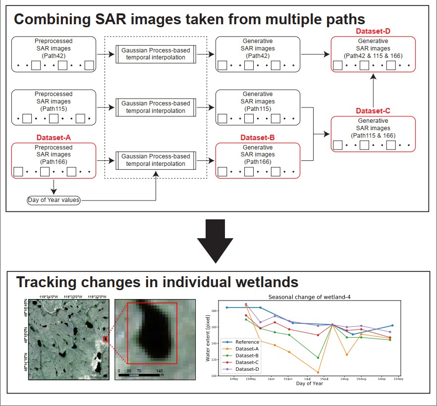
Wetland Surface Water Detection from Multipath SAR Images Using Gaussian Process-Based Temporal Interpolation

Abstract

Wetlands provide society with a myriad of ecosystem services, such as water storage, food sources, and flood control. The ecosystem services provided by a wetland are largely dependent on its hydrological dynamics. Constant monitoring of the spatial extent of water surfaces and the duration of flooding of a wetland is necessary to understand the impact of drought on the ecosystem services a wetland provides. Synthetic aperture radar (SAR) has the potential to reveal wetland dynamics. Multitemporal SAR image analysis for wetland monitoring has been extensively studied based on the advances of modern SAR missions. Unfortunately, most previous studies utilized monopath SAR images, which result in limited success. Tracking changes in individual wetlands remains a challenging task because several environmental factors, such as wind-roughened water, degrade image quality. In general, the data acquisition frequency is an important factor in time series analysis. We propose a Gaussian process-based temporal interpolation (GPTI) method that enables the synergistic use of SAR images taken from multiple paths. The proposed model is applied to a series of Sentinel-1 images capturing wetlands in Okanogan County, Washington State. Our experimental analysis demonstrates that the multiple path analysis based on the proposed method can extract seasonal changes more accurately than a single path analysis.

1. Introduction

Anthropogenic climate change has increased the damage caused by weather-related disasters, such as droughts [1]. Severe droughts can completely alter hydrological landscapes and create tipping points that alter the condition and function of individual wetlands. In some periods of severe drought, the surface water of wetlands and other water bodies may completely disappear [2]. Many regions across the globe have suffered from extreme drought [3]. One of the most vulnerable ecosystems to droughts are wetlands, which are inundated or saturated by surface or groundwater seasonally. Because wetlands provide many benefits to plants and animals, a change in flooding duration can cause a large reduction in species diversity. For example, Jolly et al. (2008) reported that some riparian tree species are vulnerable to the increase in soil salinity caused by droughts [4]. Walls et al. (2013) reported that some amphibians are sensitive to water availability and fail to breed in dried wetlands [5]. Johnson et al. (2005) reported that climate change causes habitat shifts of waterfowl in wetlands [6]. Although the importance of preserving wetlands has been well documented, landscape-level data for drought impacts are scarce [7], which is mainly because tracking changes in wetlands over weeks and months requires the installation of expensive monitoring equipment or frequent visits for field observations.

Remote-sensing technologies have the potential to reveal multitemporal wetland dynamics [8]. Many researchers have successfully detected seasonal changes in land cover using optical images, which can provide spectral information with high spatial resolution [9]. Object-based image analysis (OBIA) is especially useful for aggregating pixels and accurately delineating water shorelines [10]. The major drawback of optical data is the sensitivity to the presence of clouds and haze because optical sensors usually fail to acquire images on cloudy days. Synthetic aperture radar (SAR) has attracted substantial interest as an alternative to optical sensors because of its weather-independent characteristics. SAR consists of an active acquisition instrument that transmits microwaves and captures the signals backscattered from the earth’s surface [11]. The intensity of the backscattered signal depends on the physical (i.e., roughness) and electrical (i.e., permittivity) properties of the imaged object. Because water surfaces act as specular reflectors, microwaves entering into them are generally reflected away from the sensor, which results in a significant reduction in backscattered intensity in theory. Nevertheless, extracting water surfaces from a single SAR image is a challenging task [12] because radar backscatter from the earth’s surfaces is affected by several factors, including local incidence angle [13], speckle noise [14], soil moisture [15], and wind speed [16].

With the advances in SAR instruments, the data acquisition frequency and swath coverage have dramatically improved in the past decade. For example, the Sentinel-1 mission that includes a constellation of two SAR satellites operated by the European Space Agency (ESA) can provide high spatial resolution C-band (5.405 GHz) SAR images at a repeat cycle of 6 to 12 days [17]. Taking advantage of modern SAR missions, many researchers have successfully analyzed series of SAR images taken at different times for a variety of earth observation tasks, such as agriculture management [18,19] and disaster response [20,21]. Under the assumption that land cover remains unchanged over time, multitemporal images allow us to reduce the ambiguity of scattering mechanisms, such as speckle noise [22]. For example, in the context of open water detection, Santoro and Wegmüller reported that the combination of multitemporal images suppresses the effect of capillary waves [23]. However, the above assumption is unsuitable for most real applications because the spatial extent of ground objects may change frequently. In wetland observations, the spatial extent of water is completely different depending on acquisition timing due to the seasonal variation in precipitation. Although many methods for multitemporal image analysis for wetland monitoring have been proposed [24,25,26], few studies have successfully tracked water extent changes for individual wetlands.

In general, the number of available images and their temporal resolution are important factors in time series analysis. Unfortunately, most previous studies on wetland monitoring have utilized SAR images taken from a single path, although modern SAR missions can observe areas of interest from multiple paths. To increase the quality of time series information, we should take full advantage of multipath SAR images. The usefulness of SAR images taken from multiple paths has been demonstrated in several applications, such as deforestation detection [27] and disaster debris estimation [28]. These successes are mainly derived from the relationship between radar direction and topographic aspect as shown in Figure 1. Although multipath images can also contribute to water body detection, this approach cannot be incorporated into operational wetland monitoring in a straightforward manner because of the discrepancy in the acquisition timing of each path. Suppose that the actual water extent changes over time and we take SAR images from Path-A and Path-B as shown in Figure 2. If each path has a specific misclassification, such as radar shadow, retrieving actual changes from alternate observations is a challenging task.

One solution to this problem is to treat either acquisition path as missing data and conduct interpolation using time series information. Missing data represent a common issue in almost every real dataset, and this problem has been thoroughly studied from a statistical perspective [29]. In the field of remote sensing, mismatched acquisition dates have occasionally been discussed in relation to a fusion of optical and SAR time series [30,31]. For example, Reiche et al. (2015) proposed a deforestation detection method that uses a weighted regression model to interpolate missing observations of Landsat and ALOS PALSAR [32]. Stendardi et al. (2019) linearly interpolated scarce time series of Sentinel-1 and Sentinel-2 data to monitor meadows on mountains [33]. Pipia et al. (2019) used a Gaussian process for the synergistic use of Sentinel-1 and Sentinel-2 to estimate the leaf area index from a series of images [34]. The application of multipath analysis to nonstationary environments requires the interpolation of missing observations. However, when interpolating a series of SAR images that capture wetlands, we must consider the possibility that the recorded intensity is affected by several types of noise. Moreover, the water extent may change dramatically between image acquisitions.

To overcome this problem, this research proposes a Gaussian process-based temporal interpolation (GPTI) method. The Gaussian process is a supervised learning method that formulates the learning of a regressor within a Bayesian framework [35]. When solving a regression problem, the Gaussian process enables us to reconstruct the underlying function by removing contaminating factors. The advantage of the Gaussian process is that such regressions can be performed exactly using matrix operations. In the field of remote sensing, this stochastic approach has been successfully applied to several real applications. For example, Savory et al. (2017) proposed a Gaussian process-based model to measure urbanization trends based on nighttime light imagery [36]. Pasolli et al. (2010) applied the Gaussian process to datasets obtained from multispectral medium-resolution imaging spectrometers to estimate chlorophyll concentrations in subsurface waters [37]. In our method, retrieved series SAR images from each path are coregistered so that the time series of each pixel can be extracted. Subsequently, the underlying relationships between day of year and extracted time series are reconstructed using the Gaussian process at each pixel. Based on our assumption, the Gaussian process enables the interpolation between any observation and simulation of generative SAR images, which eliminates the discrepancy of multipath acquisition. Therefore, the proposed method has the potential to detect wetland water bodies using multipath images, even if surface conditions change dramatically.

To validate our assumption, we apply the proposed model to a series of Sentinel-1 images that capture wetlands in Washington State, United States during the dry season in 2018. These wetlands are known to suffer from recent severe droughts. The accuracy of detecting water bodies is evaluated using reference data derived from Sentinel-2 images obtained during the same period. To gain a deeper understanding of the proposed model, this study experimentally conducts water body detection analysis under several conditions.

2. Study Area and Dataset

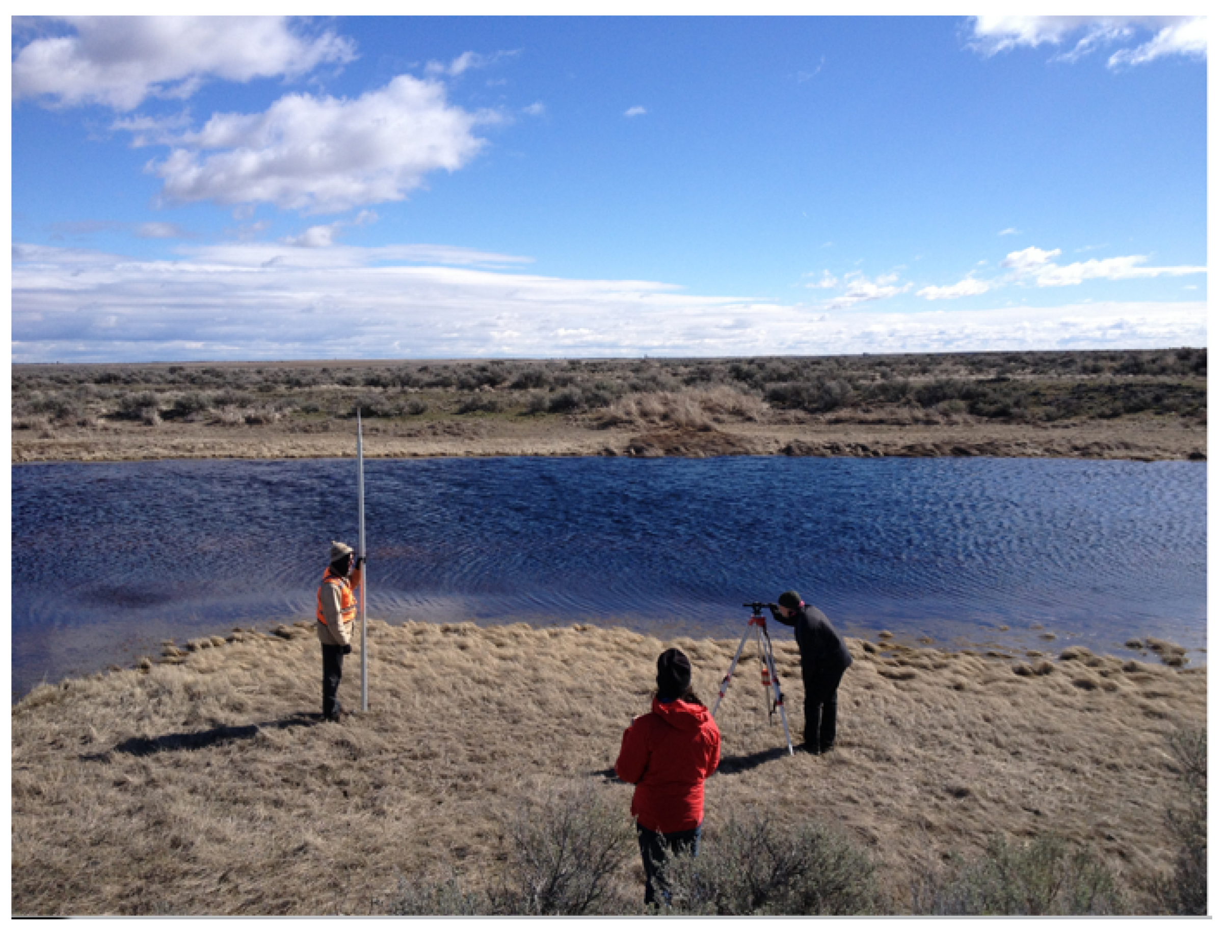
2.1. Study Area—Okanogan County, WA, US

The southern part of Okanagan County, Washington (United States), which belongs to the Columbia Plateau ecoregion, was selected as the study area (Figure 3). Because this ecoregion is home to a number of threatened species, including sharp-tailed grouse (Tympanuchus phasianellus) and pygmy rabbit (Brachylagus idahoensis), conservation planning has attracted considerable interest [38,39]. Our study area is located approximately 20 kilometers south of Omak. A summary of the climate statistics in Omak is shown in Figure 4. As shown in Figure 5, the surface of our study area is covered by sparse vegetation, including sagebrush (Artemisia tridentata), because the rain shadow of the Cascade Mountains limits the amount of precipitation, which results in a semiarid climate [40]. The wetlands in the study area generally fill up during the winter months and draw down in the drier summer months. Because of glacial tills that were sedimented during the last ice age, the surface water of the wetlands rarely interacts with the ground water [41]. These wetlands mainly depend on precipitation as their source of water and are known to be vulnerable to climate change. Moreover, anthropogenic impacts, such as farming and grazing, make them a high-priority area for conservation.

2.2. Sentinel-1 Images

The overlapping observations of Sentinel-1 enable us to obtain SAR images from multiple paths. In the case of our study area, SAR images can be obtained from four types of acquisition geometry as shown in Figure 3. The properties of each acquisition path are summarized in

Table 1. Properties of each acquisition path that can capture our study area.

	Platform	Orbit	Local Iincidence Angle
Path42	Sentinel-1B	Descending	43.4$°$
Path64	Sentinel-1B	Ascending	43.9$°$
Path115	Sentinel-1B	Descending	34.5$°$
Path166	Sentinel-1B	Ascending	35.0$°$

. This study uses images taken from Path42, Path115 and Path166 because many observations from Path64 were skipped in 2018 because of onboard satellite problems. In total, 39 images acquired in interferometric wideswath (IW) mode from April 2018 to September 2018 are selected for analysis (Figure 6) The ground range detected (GRD) products of these images can be downloaded from the Copernicus Open Access Hub (https://scihub.copernicus.eu/dhus/#/home). They have a spatial resolution of approximately $20\mathrm{m}\times 22\mathrm{m}$ in the ground range and azimuth direction.

Downloaded data were preprocessed using the Python module snappy (Version 6.0.10), which enables access to the Sentinel Application Platform (SNAP) Java API from Python scripts (Version 3.6.8). Preprocessing steps include orbit correction, calibration, Lee filtering ($3\times 3$), geometric correction, coregistration and conversion to decibel scale. In orbit correction, the satellite position at image acquisition is modified using auxiliary files provided by the ESA. Subsequently, radar brightness is calibrated and converted into radar reflectivity per unit area. Using Lee filtering, we can mitigate speckle noise generated by the random interference of many elementary reflectors within a unit area [42]. In the geometric correction, preprocessed images are resampled to a 10 m grid and projected onto UTM 10N/WGS84 based on the Shuttle Radar Topography Mission-based digital elevation model [43]. Projected images are coregistered using bilinear interpolation so that the time series of each pixel can be extracted. Note that our study area basically does not include steep slopes. If area of interest have topographical variations that cause serious layover, an advanced coregistration method should be incorporated into the preprocessing. Finally, the intensity of each pixel is converted to a logarithmic scale. Examples of preprocessed SAR images are shown in Figure 7. As shown in these figures, SAR images taken from Path166 have different shadowing properties than those from Path42 and Path115 because of the orbit direction. Additionally, because Path42’s incident angle is larger than Path115’s incident angle, the average intensity of the example images of Path42 is lower than the average intensity of the example images of Path115.

2.3. Sentinel-2 Images

Sentinel-2 is an Earth observation satellite operated by the ESA that provides 10 m resolution multispectral images around the world [44]. Because the appearance of clouds degrades the quality of optical images, this study uses only 6 cloud-free Sentinel-2 images that capture our study area during the period (Figure 6). The original data can be downloaded from Copernicus Open Access Data Hub and are typically in the form of Level-1C products, which record top-of-atmosphere reflectance [44]. These products are converted into Level-2A products, which record bottom-of-atmosphere reflectance, using the ESA’s Sen2Cor module (Version 2.5.5) [45]. This module implements atmospheric corrections based on the atmospheric precorrected differential absorption algorithm [46]. Sentinel-2 images are also terrain-corrected using the Shuttle Radar Topography Mission-based digital elevation model and projected onto UTM 10N/WGS84.

Subsequently, these images were converted into reference data that include water masks and land masks. We first visually inspected the Sentinel-2 image taken on 22 July 2018, and each pixel was manually classified as either a water pixel or land pixel. Manually annotated pixels were used to train a pixel-based logistic regression model that used blue, green, red, and near-infrared reflectance as features. Although pixel-based classification ignores the spatial context and might cause the mixed pixel problem [47], this problem is negligible compared to the complexity of Sentinel-1 images. Before creating reference data, we conducted a field survey around our study area. Using photographs we took in field survey, we manually selected training points that obviously belong to water or land pixels in a Sentinel-2 image. Subsequently, a classifier for Sentinel-2 images was trained. In this study, water pixels in reference data include open water surface and submerged area. The trained classifier was applied to all the images, and the classification results were treated as reference data. The preprocessed Sentinel-2 images and derived reference data are shown in Figure 8.

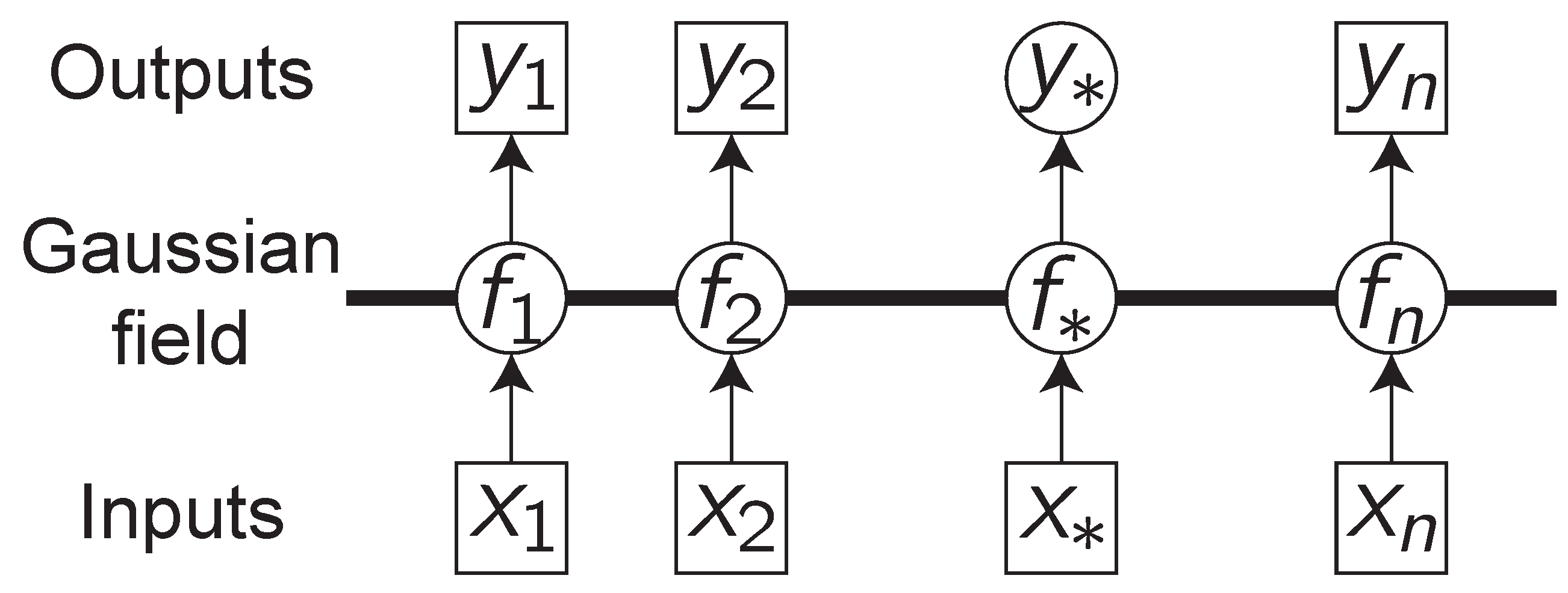
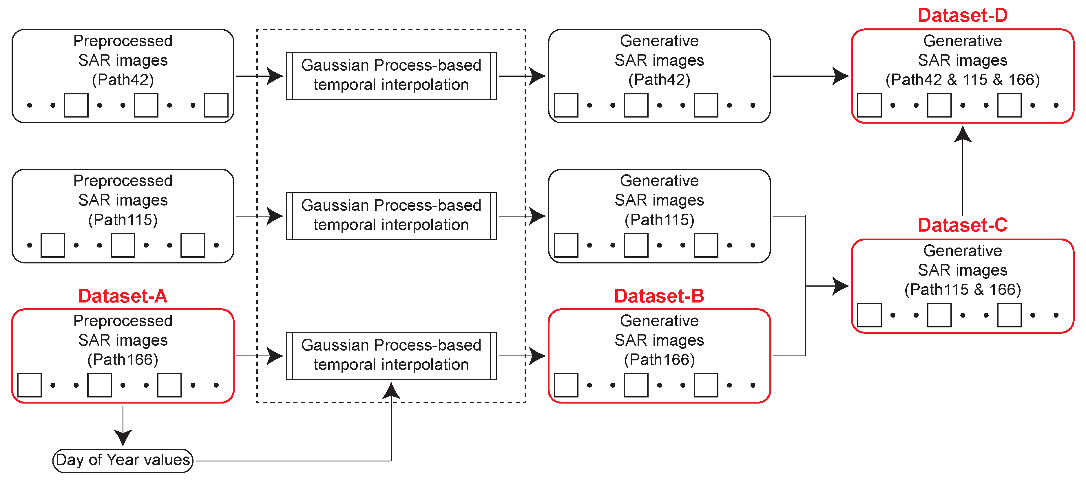
3. Gaussian Process-Based Temporal Interpolation (GPTI)

3.1. Mathematical Formulation of the Gaussian Process

Let $\mathbf{x}={\left(x_1,x_2,\dots ,x_n\right)}^{\mathrm{T}}$ be the input variables of the training data, and let $\mathbf{y}={\left(y_1,y_2,\dots ,y_n\right)}^{\mathrm{T}}$ be the output variables of the training data. The final goal is to estimate an underlying function $\mathbf{f}$. In Gaussian process regression, the underlying function $\mathbf{f}$ is defined as a collection of random variables, any finite number of which have a joint Gaussian distribution $N\left(\mu ,\mathbf{K}\right)$, where $\mu$ is the mean of the output variables. A graphical model representation of a Gaussian process is given in Figure 9.

Hereafter, the input variables are normalized such that $\mu =0$ for simplicity. Elements of the covariance matrix are given as a kernel function $k_{ij}\left(x_i,x_j\right)=\varphi {\left(x_i\right)}^{\mathrm{T}}\varphi \left(x_j\right)$. This study uses the radial basis kernel function, which can be defined as

$$\begin{array}{ccc}\hfill k_{ij}\left(x_i,x_j\right)& =& {\theta }_{1}exp\left(-\frac{1}{2{\theta }_2^2}{|x_i-x_j|}^2\right)\hfill \end{array}$$

where ${\theta }_1$ and ${\theta }_2$ are a scale parameter and a length parameter, respectively. Depending on the length parameter, the covariance is almost unity between variables whose corresponding inputs are very close and decreases as their distance in the input space increases. In practice, we must select or develop an appropriate kernel function so that prior knowledge is incorporated into the regression. If the output variables have a downward or upward trend relative to the input variables, a nonstationary covariance function can be selected [48]. If the output variables have periodic dependency on the input variables, a periodic covariance function can be selected [49].

Supposing that Gaussian noise is added to the observations, the output variables can be denoted as $\mathbf{y}={\mathbf{f}}_x+N\left(0,{ϵ}^2\mathbf{I}\right)$. The conditional distribution of $\mathbf{y}$ given $\mathbf{x}$ can be expressed as follows:

$$\begin{array}{ccc}\hfill P\left(\mathbf{y}|\mathbf{x}\right)& =& \int P\left(\mathbf{y}|\mathbf{f}\right)P\left(\mathbf{f}|\mathbf{x}\right)d\mathbf{f}\hfill \\ & =& N\left(\mathbf{0},\mathbf{K}+{ϵ}^2\mathbf{I}\right)=N\left(\mathbf{0},{\mathbf{K}}^{\prime }\right)\hfill \end{array}$$

A component covariance matrix ${\mathbf{K}}^{\prime }$ can be defined as

$$\begin{array}{ccc}\hfill k_{ij}^{\prime }\left(x_i,x_j\right)& =& {\theta }_{1}exp\left(-\frac{1}{2{\theta }_2^2}{|x_i-x_j|}^2\right)+{\theta }_3\delta \left(x_i,x_j\right)\hfill \end{array}$$

where ${\theta }_3={ϵ}^2$. Considering the above equations, we predict the output variable $y^{\ast }$ for new input variable $x^{\ast }$. To begin, the joint probability of the training data and testing data can be written as

$$\begin{array}{ccc}\hfill P\left(\begin{array}{c}\mathbf{y}\\ y^{\ast }\end{array}|\begin{array}{c}\mathbf{x}\\ x^{\ast }\end{array}\right)& =& N\left(\mathbf{0},\left(\begin{array}{cc}{\mathbf{K}}^{\prime }& {\mathbf{k}}_{\ast }\\ {\mathbf{k}}_{\ast }^{\mathrm{T}}& k^{\prime }\left(x^{\ast },x^{\ast }\right)\end{array}\right)\right)\hfill \end{array}$$

where ${\mathbf{k}}_{\ast }={\left(k\left(x^{\ast },x_1\right),k\left(x^{\ast },x_2\right),\dots ,k\left(x^{\ast },x_n\right)\right)}^{\mathrm{T}}$. For prediction purposes, the conditional distribution of $y^{\ast }$ given $x^{\ast }$, $\mathbf{x}$ and $\mathbf{y}$ must be computed. Notably, this distribution also follows a multivariate Gaussian distribution with the following mean and variance.

$$\begin{array}{ccc}\hfill P\left(y^{\ast }|x^{\ast },\mathbf{x},\mathbf{y}\right)& =& N\left({\mathbf{k}}_{\ast }^{\mathrm{T}}{\mathbf{K}\prime }^{-1}\mathbf{y},k^{\prime }\left(x^{\ast },x^{\ast }\right)-{\mathbf{k}}_{\ast }^{\mathrm{T}}{\mathbf{K}\prime }^{-1}{\mathbf{k}}_{\ast }\right)\hfill \end{array}$$

The predictive mean is a linear combination of observations $\mathbf{y}$. The advantage of the Gaussian process formulation is that the combination of the prior and noise models can be calculated exactly using matrix operations. This solution is the same as that obtained for kernel ridge regression, where the noise variance term appears as the regularization factor. [50] provided a comprehensive review of the differences between the Gaussian process and kernel ridge regression. Compared with kernel ridge regression, the type-2 maximum likelihood can be applied to the Gaussian process to optimize hyperparameters $\mathit{\theta }=\left({\theta }_1,{\theta }_2,{\theta }_3\right)$ automatically. The negative log marginal likelihood of the training data can be expressed as follows.

$$\begin{array}{ccc}\hfill logp\left(\mathbf{y}|\mathbf{x},\mathit{\theta }\right)& =& logN\left(\mathbf{y}|\mathbf{0},{\mathbf{K}}^{\prime }\right)\hfill \\ & =& -\frac{n}{2}log\left(2\pi \right)-\frac{1}{2}log\left|{\mathbf{K}}^{\prime }\right|-\frac{1}{2}{\mathbf{y}}^{\mathrm{T}}{\mathbf{K}\prime }^{-1}\mathbf{y}\hfill \end{array}$$

Notably, we can analytically express the partial derivatives of the log likelihood, which forms the basis of an efficient learning scheme.

$$\begin{array}{ccc}\hfill \frac{\partial logp\left(\mathbf{y}|\mathbf{x},\mathit{\theta }\right)}{\partial {\mathit{\theta }}_j}& =& -\frac{1}{2}\mathrm{Tr}\left({\mathbf{K}\prime }^{-1}\frac{\partial {\mathbf{K}}^{\prime }}{\partial {\theta }_j}\right)+\frac{1}{2}{\mathbf{y}}^{\mathrm{T}}{\mathbf{K}\prime }^{-1}\frac{\partial {\mathbf{K}}^{\prime }}{\partial {\theta }_j}{\mathbf{K}\prime }^{-1}\mathbf{y}\hfill \end{array}$$

Gradient-based optimization, such as the scaled conjugate gradient (SCG) [51], enables updating of these parameters. Because these parameters can converge to local minima, the initial values and ranges must be selected carefully.

3.2. Applying GPTI to Preprocessed SAR Images

A graphical overview of the proposed method is shown in Figure 10. Series of SAR images are coregistered first so that the time series of each pixel can be extracted. Subsequently, the Gaussian process is applied to each time series to obtain a regression function whose input value x corresponds to the day of the year and output value y corresponds to intensity. Note that this regression function is estimated in each polarization (VH and VV) separately. The initial values of parameters ${\theta }_1$, ${\theta }_2$ and ${\theta }_3$ are set to 1, 10 and 10, respectively. The variable range of these parameters is [0.01, 100]. These hyperparameters are updated at each pixel using evidence approximation. Afterward, a fully interpolated image stack can be obtained by combining all the estimated functions, and we can reconstruct generative SAR images. In this study, the Gaussian process was implemented using the Python module Scikit-Learn (Version 0.21.2).

Examples of generative SAR images based on the proposed method are shown in Figure 11. Four types of classification datasets are compared in terms of water detectability in the following sections, and they are created based on a combination of acquisition paths. Figure 12 provides an overview of the workflow for dataset creation. Dataset-A consists of series of preprocessed SAR images taken from Path166. By applying the proposed interpolation to each path image, we can reconstruct generative SAR images whose acquisition timings are the same as those of Path166. To verify the effect of the Gaussian process itself, we defined generative SAR images from Path166 as Dataset-B. Dataset-C consists of a combination of generative images from Path115 and Path166, and Dataset-D consists of a combination of generative images from Path42, Path115 and Path166. Note that in path-combined datasets, such as Dataset-C, each pixel has multiple dual-polarization values. For example, the SAR images in Dataset-C have four pixel values: VH-Path115, VV-Path166, VH-Path115 and VV-Path166.

4. Experimental Analysis

A schematic overview of the experimental analysis is shown in Figure 13. Our experimental analysis can be separated into two parts. In the first part, we create a water body classifier for each dataset. A pair of Sentinel-1 and Sentinel-2 images taken on 22 July 2018 are treated as training data in our analysis. In the training phase, all of the pixels are split into two categories, with one for estimating coefficients the of classification and the other for producing the error matrix. This error matrix can provide insights into the classification model, although spatial data leakage may limit independency of error matrix derived from 22 July 2018 [52]. Subsequently, images taken on 22 May 2018 are used for further validation, which is completely independent from training data. As shown in Figure 6, the acquisition timing of Sentinel-1 and Sentinel-2 does not match due to the confliction of revisit time. Thus, we only use Sentinel-2 images taken on 22 May 2018 and 23 July 2018 to produce the error matrix because Sentinel-1 images taken on the same date are available. In the second part, we apply the trained model to all the images in each dataset. A series of water maps derived from the classification is used to construct surface-water hydrographs for the selected wetlands. In the following two subsections, we will provide details of the analyses. Note that these procedures are implemented using Python (Version 3.6.8).

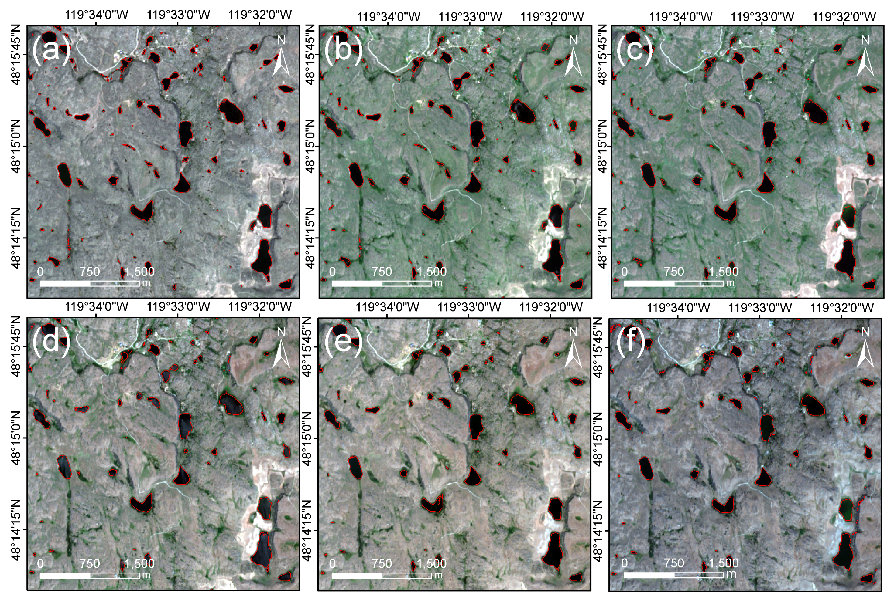
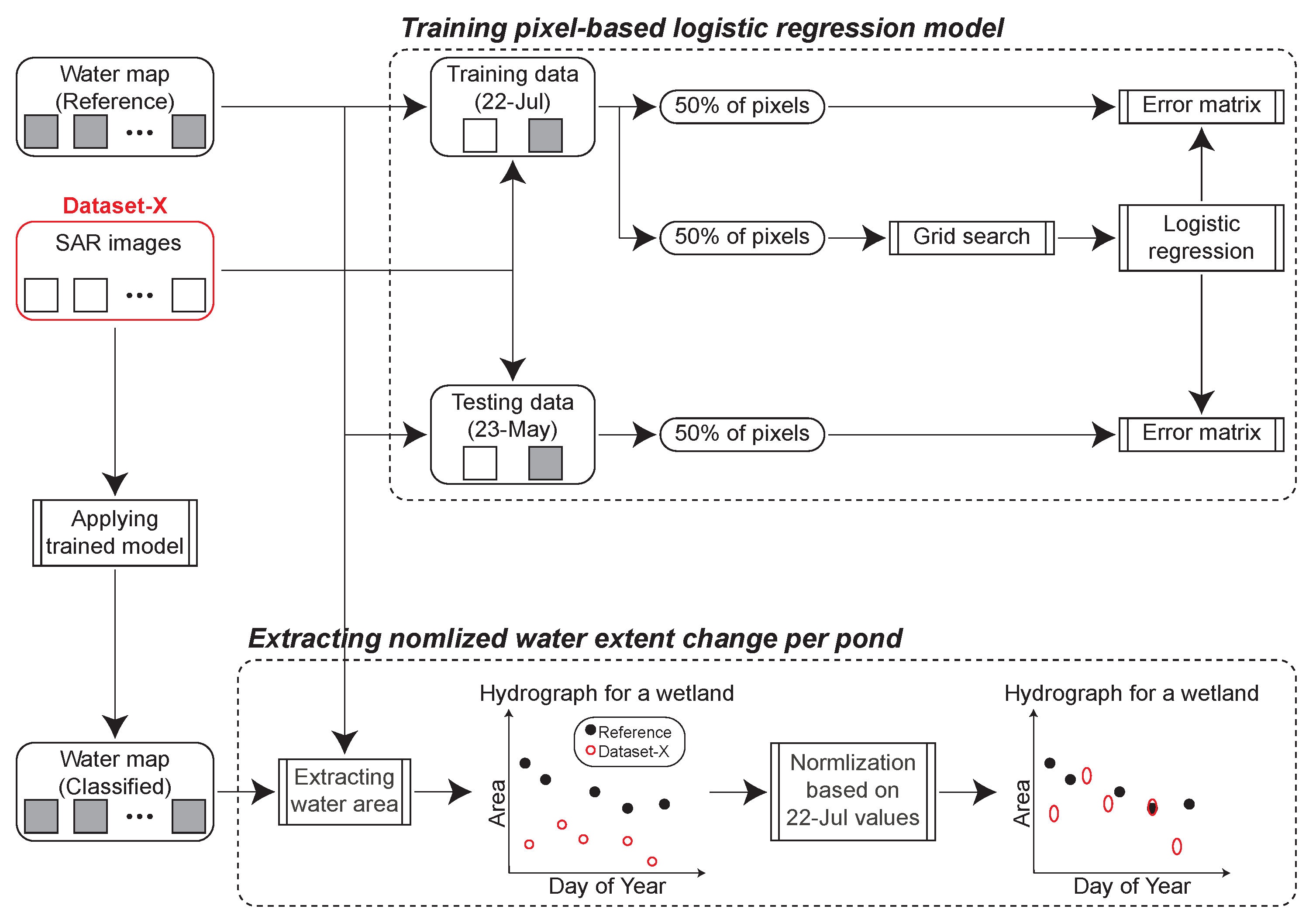
4.1. Water Body Classification

This study uses logistic regression for pixel-based water body classification. As discussed previously, the number of intensities used as input values $\mathbf{x}={\left(x_1,x_2,\dots ,x_i\right)}^{\mathrm{T}}$ differs depending on the dataset. Suppose that a subset of training data is ${\left\{\left({\mathbf{x}}_i,y_i\right)\right\}}_{i=1}^N$, where $y_i\in \left\{0,1\right\}$ is the true label derived from the reference data. Half of the pixels within the image are randomly selected for training data, and the other half of the dataset is used for testing. The output value of the model, which corresponds to the probability that a pixel belongs to the water mask (i.e., $y=1$), can be defined as

$$\begin{array}{c}\hfill \mathrm{Pr}\left[y=1|\mathbf{x},\mathit{\omega },b\right]=\frac{1}{1+exp(-{\mathit{\omega }}^{\mathrm{T}}\mathbf{x}-b)}\end{array}$$

where $\mathit{\omega }$ and b are parameters estimated using the maximum likelihood method. The objective function we need to minimize is defined as

$$\begin{array}{c}\hfill E\left(\mathit{\omega },b\right)=-Clog\sum _{i=1}^N\mathrm{Pr}\left[y_i|{\mathbf{x}}_i,\mathit{\omega },b\right]+\frac{1}{2}\left({\mathit{\omega }}^{\mathrm{T}}\mathit{\omega }+b^2\right)\end{array}$$

where C is a regularization factor to prevent overfitting. To select this hyperparameter, a 5-fold cross validation grid search is applied to the training data. The range of C is set to ${log}_{10}C\in \{-4,-3.5,-3,\dots ,4\}$. Subsequently, classification parameters $\mathit{\omega }$ and b are trained using training data. An error matrix derived from the testing dataset is used to quantitatively assess the overall accuracy and F-score, which is the harmonic mean of precision and recall [53]. Let $TP$, $FP$, $TN$ and $FN$ be a number of true positives, false positives, true negatives and false negatives. The F-score can be calculated as follows.

$$\begin{array}{ccc}\hfill \mathrm{Precision}& =& \frac{TP}{TP+FP}\hfill \\ \hfill \mathrm{Recall}& =& \frac{TP}{TP+FN}\hfill \\ \hfill \mathrm{Fscore}& =& \frac{2·\mathrm{Precision}·\mathrm{Recall}}{\mathrm{Precision}+\mathrm{Recall}}\hfill \end{array}$$

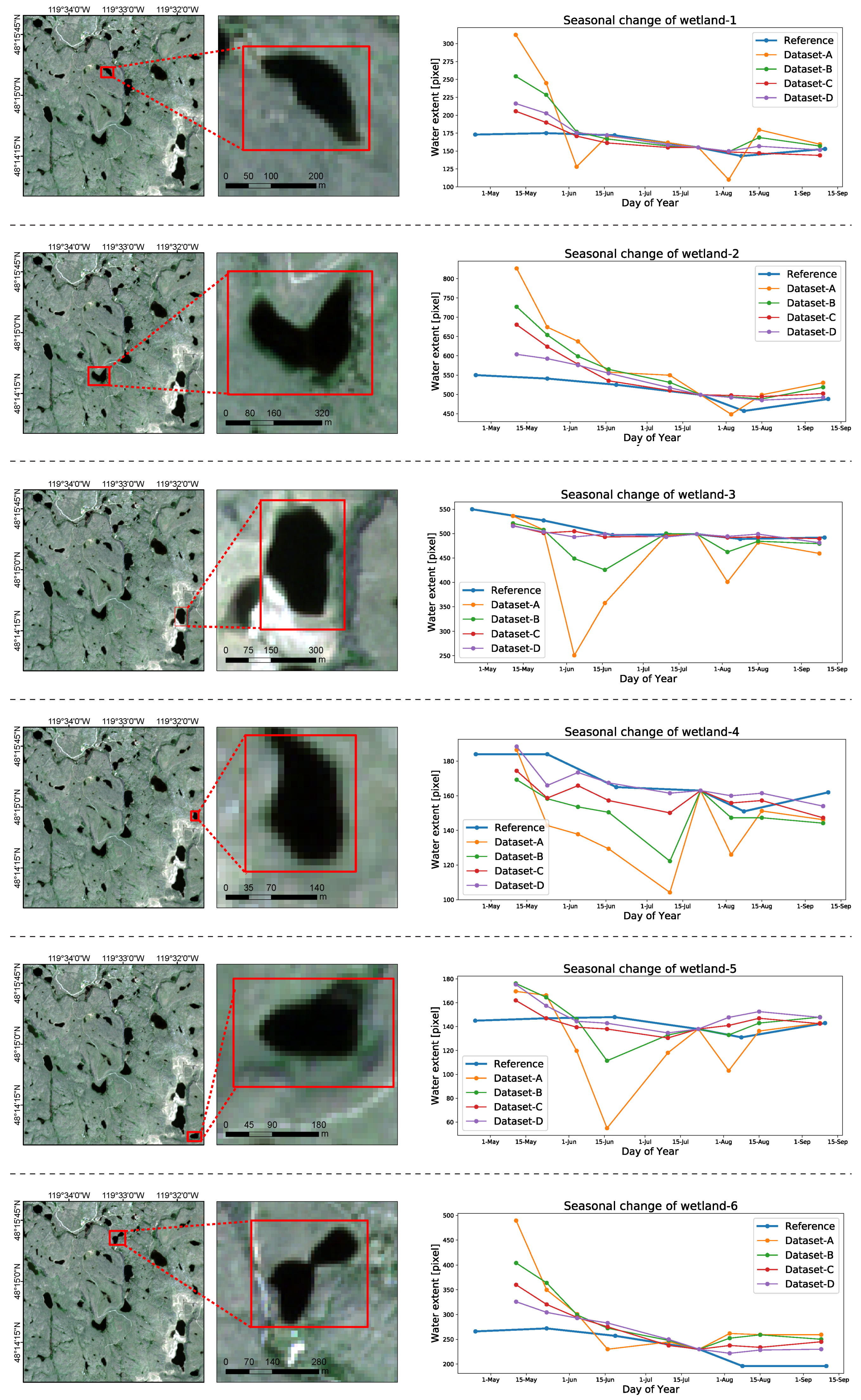
4.2. Extracting Seasonal Water Extent Change

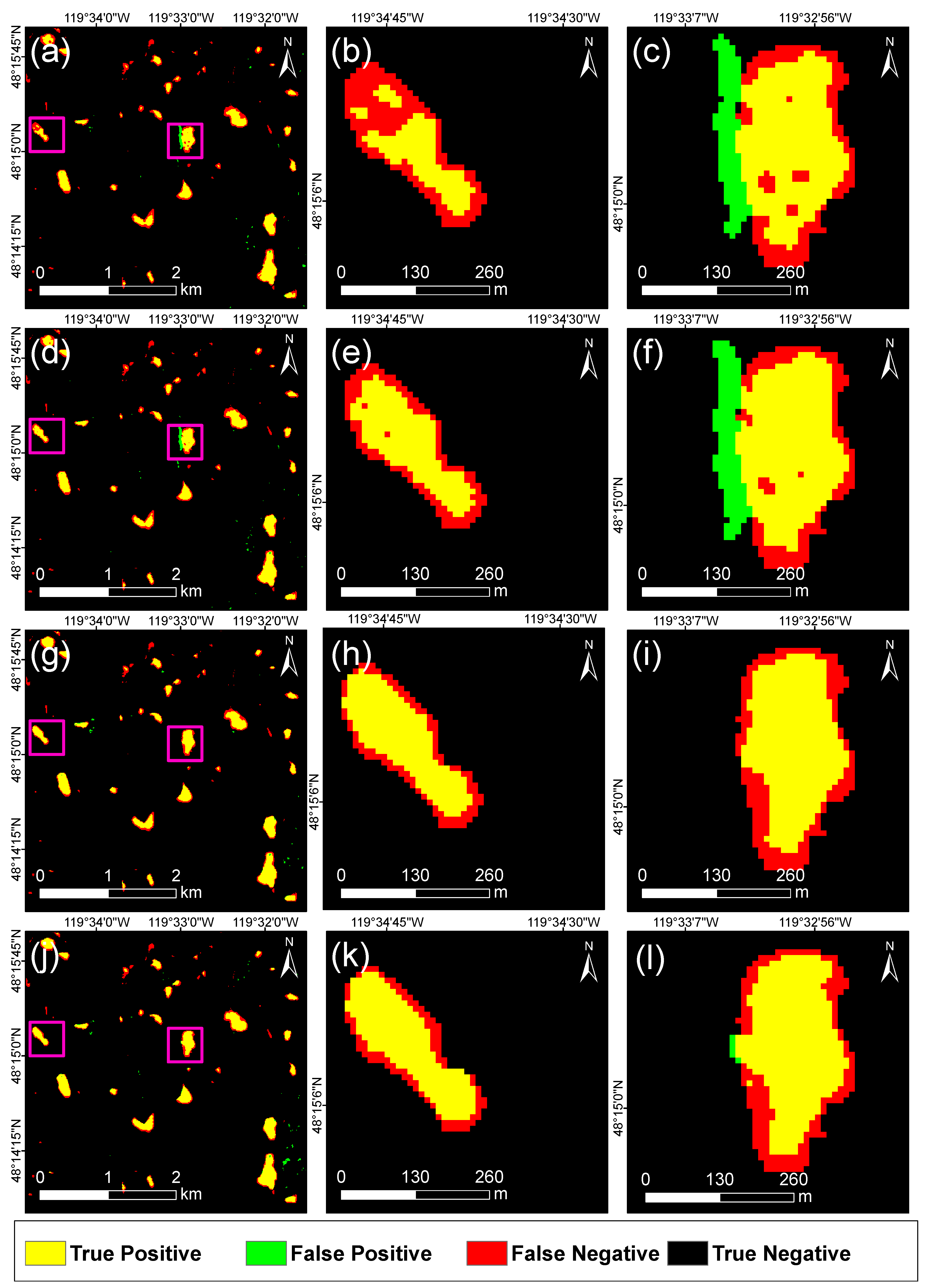
The trained model is applied to all images in each dataset to obtain 10 water maps. As shown in Figure 6, because available Sentinel-2 images range from 25 April 2018 to 10 September 2018, we omit generative images taken on 25 April 2018 and 20 September 2018. The water maps derived from the classification enable reconstruction of surface-water hydrographs for each pond with better temporal resolution than that provided by Sentinel-2-based reference data. In this study, we selected 6 ponds for water extent tracking as shown in Figure 14. In each water map, the number of pixels within a target rectangle that are classified as water are counted.

Subsequently, the transitions of the water areas are visualized. To validate the derived transition graphs, we also extract seasonal changes from the Sentinel-2 image stack. Note that the acquisition dates of Sentinel-2 do not match those of Sentinel-1 except for 22 July 2018. Thus, the consistency between the water extent derived from classification and reference data is visually verified. To mitigate misestimations derived from the flooding boundary, we normalize the water extent using Sentinel-1 and Sentinel-2 images taken on 22 July 2018 as the reference water extent. Let the water area estimated from Sentinel-1 and Sentinel-2 images be x pixels and y pixels, respectively. In this case, the normalized coefficient N is the ratio of x to y. This coefficient is computed for each pond and multiplied by the estimated water extent when drawing the seasonal change figures.

5. Results

The coefficients of the logistic regression motel estimated from training data are summarized in

Table 2. Coefficients and bias estimated from training data.

		Dataset-A	Dataset-B	Dataset-C	Dataset-D
Coefficients of original intensity	${\omega }_{166\left(\mathrm{VH}\right)}$	−0.52
	${\omega }_{166\left(\mathrm{VV}\right)}$	−0.57
Coefficients of generative images	${\omega }_{166\left(\mathrm{VH}\right)}$		−0.68	−0.42	−0.28
	${\omega }_{166\left(\mathrm{VV}\right)}$		−0.53	−0.30	−0.38
	${\omega }_{115\left(\mathrm{VH}\right)}$			−0.42	−0.22
	${\omega }_{115\left(\mathrm{VV}\right)}$			−0.33	−0.53
	${\omega }_{42\left(\mathrm{VH}\right)}$				−0.46
	${\omega }_{42\left(\mathrm{VV}\right)}$				0.46
Bias	b	−22.34	−25.26	−28.93	−29.64

. Note that, the number of images combined for classification differs depending on datasets. Empty fields in the table means corresponding intensities are not used for classification. For example, the logistic regression model for Dataset-C can be described as

$$\begin{array}{c}\hfill \frac{1}{1+exp(0.47x_{166\left(\mathrm{VH}\right)}-0.42x_{166\left(\mathrm{VV}\right)}+0.13x_{115\left(\mathrm{VH}\right)}+0.51x_{115\left(\mathrm{VV}\right)}+28.92)}\end{array}$$

where VH and VV intensity in the SAR images taken from Path166 are denoted as $x_{166\left(VH\right)}$ and $x_{166\left(VV\right)}$, respectively, and VH and VV intensity in the SAR images taken from Path115 are denoted as $x_{115\left(VH\right)}$ and $x_{115\left(VV\right)}$, respectively. The validity of estimated parameters will be discussed later.

Visual comparisons between reference data and classification results of 22 July 2018 and 23 May 2018 are summarized in Figure 15 and Figure 16, respectively, in which the true positives, false positives, false negatives, and true negatives are marked in yellow, green, red and black, respectively. Error matrices derived from the testing data in 22 July 2018 and 23 May 2018 are shown in

Table 3. Error matrices derived from images taken on 22 July 2018.

		Reference Data
		Water	Land
Classified	Water	2062	120	F-score
(Dataset-A)	Land	1671	82,260	69.7%
Classified	Water	2114	113	F-score
(Dataset-B)	Land	1479	82,407	73.5%
Classified	Water	2390	48	F-score
(Dataset-C)	Land	1314	82,361	77.8%
Classified	Water	2434	82	F-score
(Dataset-D)	Land	1281	82,316	78.1%

and

Table 4. Error matrices derived from images taken from 23 May 2018.

		Reference Data
		Water	Land
Classified	Water	2509	111	F-score
(Dataset-A)	Land	1850	81,643	71.9%
Classified	Water	2615	134	F-score
(Dataset-B)	Land	1725	81,639	73.8%
Classified	Water	2676	8	F-score
(Dataset-C)	Land	1613	81,816	76.8%
Classified	Water	2823	12	F-score
(Dataset-D)	Land	1566	81,712	78.2%

, respectively. These tables demonstrate two interesting outcomes. First, the synergistic use of multipath images increases the water mapping accuracy. For example, Dataset-C (F-score = 77.8% in 22 July 2018 and F-score = 76.8% in 23 May 2018) is superior in terms of water detectability to Dataset-B (F-score = 73.5% in July and F-score = 73.8%). This superiority is partly because the number of false positives in Dataset-C (48 pixels in 22 July 2018 and 8 pixels in 23 May 2018) is drastically reduced compared to the number of false positives in Dataset-B (113 pixels in 22 July 2018 and 134 pixels in 22 May 2018). Interestingly, a similar reduction tendency is observed in (f) and (i) of Figure 15 and in (f) and (i) of Figure 16. Second, applying the GPTI increases water detectability without combining multipath images. Dataset-B is superior in terms of its ability to detect water to Dataset-A (F-score = 69.8% in 22 July 2018 and F-score = 71.9% in 23 May 2018), although both datasets use images taken from a single path. This superiority is partly because the number of false negatives in Dataset-B (1479 pixels in 22 July 2018 and 1725 pixels in May 23) is slightly reduced compared to the number of false negatives in Dataset-B (1314 pixels in 22 July 2018 and 1613 pixels in May 23). As shown in (b) and (e) of Figure 15, a similar trend is observed in the graphical comparison. However, in (b) and (e) of Figure 16, such a tendency cannot be confirmed in the wetland.

The extracted seasonal changes for each pond are shown in Figure 17. According to these figures, the water extent estimated from Dataset-A is unnaturally fluctuating and sometimes much lower than the reference data; moreover, the water extent estimated from Dataset-A of wetland-3 on 4 June 2018 is completely different from the reference data. Although the water extents estimated from Dataset-B are more similar to the actual changes, they often show the same tendency as that of Dataset-A (i.e., sudden decrease) in some wetlands, such as wetland-5. Note that both datasets use SAR images taken only from Path166, and the difference is whether the Gaussian process is applied. Compared with the error matrices, significant differences between Dataset-C and Dataset-D are not observed. Dataset-C and Dataset-D both occasionally capture the wetland changes more accurately. This trend is remarkable, especially in the surface-water hydrographs for wetland-2 and wetland-4. However, these datasets allow us to reconstruct water extent changes with a higher accuracy than Dataset-A and Dataset-B.

6. Discussion

Coefficients of classification are discussed in this paragraph. Most of the coefficients took negative values as shown in Table 2. Such coefficients increase the pixel’s probability of inundation if the corresponding polarization has low intensity. However, the coefficient ${\omega }_{42\left(VV\right)}$ only took a positive value. This result can be explained by considering complex backscatter from inundated vegetation. Basically, inundated vegetation induces a combination of double-bounce and volume backscattering [54]. Cazals et al. (2016) also used Sentinel-1 images to monitor coastal marsh. Their study reported that flooded grassland shows higher VV intensity than non-flooded grassland [24]. Interestingly, significant differences in VH intensity were not observed from their study area. As discussed in Section 2, our study area does not support tall trees. The vegetation in our study area causes similar backscattering effects as observed in their study area. Thus, the combination of positive coefficients ${\omega }_{42\left(VV\right)}$ and negative coefficients ${\omega }_{42\left(VV\right)}$ can be interpreted as the index for detecting inundated vegetation. Note that we designed a simple classification scheme (i.e., linear discriminator) to investigate the effect of the GPTI. From an electrical scattering perspective, we should incorporate the polarization ratio in the classification model [55]. As shown in Figure 15 and Figure 16, most of the omission errors occur around the edge of wetlands. Such misclassifications are seemingly derived from the limitation of the linear discriminator, which results in an underestimation of the water extent. However, the amount of such misclassifications seems to be proportional to the size of wetland in our study area. Thus, normalization of the time series, which is described in Figure 13, enables the extraction of seasonal variation among individual wetlands.

There are no noticeable differences between the original preprocessed SAR images (Figure 7) and generative SAR images (Figure 11). However, our experimental water body detection shows that we can detect water bodies more accurately from generative images than from original images. This improvement can be considered in terms of the effect of capillary waves on water. As discussed in the introduction, wind-roughened surface water shows high backscatter intensity in original SAR images. Such open water may be misclassified as land due to the effect of capillary waves. In our understanding, because the location of the capillary wave differs depending on the weather conditions at the acquisition time, (e) Figure 16 does not include considerable false negative pixels. Although generative images are effective for water mapping for the above reason, the wind effect is not entirely removed. For example, extremely roughened water, whose intensity contaminates a regression function, may still lead to the underestimation of the water extent. We believe that this is the reason that the water-surface hydrographs of Dataset-A and Dataset-B show a similar sudden declining tendency.

Our experimental analysis also demonstrated that multipath analysis can reveal wetland dynamics more accurately than monopath analysis. This effect can be justified from two perspectives: the diversity of the radar direction and the probability of emergence of wind-roughened water. First, combining ascending and descending images dramatically increases the method’s ability to detect water because misclassifications derived from the shadowing effect can be mitigated. In the visual comparison map of Dataset-B, false positive pixels in (c) and (f) of Figure 15 and in (c) and (f) of Figure 16 clearly correspond to shadow areas in (c) and (f) of Figure 11. These pixels are successfully classified in Dataset-C because of the combination of different radar directions. We can mask the radar shadow using a ray tracing method in theory when high-resolution topographical models are available [56]. Moreover, incorporating high-quality elevation data into classification algorithms increases the detectability of water bodies [57]. Unfortunately, the high cost of operating airborne scanners limits the use of high-resolution elevation models for water detection. In relation to the diversity of radar direction, we should discuss why there are no differences between the F-scores of Dataset-C and Dataset-D. This lack might be related to the lower importance of the incident angle difference between Path42 and Path115 relative to the range direction difference. Second, when more intensities derived from several paths are considered as feature values, water pixels are less frequently misclassified as land pixels. As shown in Figure 17, even if Dataset-B and Dataset-C are affected by underestimations due to the wind effect, Dataset-D provides accurate information.

As we mentioned in the introduction, many studies have conducted multiple SAR images for wetland monitoring. Compared to these studies, our approach enables the detection of temporal changes of wetlands in detail. Most previous research studies have utilized multi-temporal images to improve the accuracy of land cover mapping by sacrificing the temporal resolution of the analysis. For example, Furtado et al. (2016) demonstrated that dual-season (i.e., dry season and rainy season) Radarsat-2 images can be used to map flooded vegetation in wetlands [58]. Banks et al. (2019) reported that using dual-season Radarsat-2 images taken from different angles further improves the accuracy for wetland mapping [59]. The critical problem is that these approaches do not provide time series variations of land cover change between seasons. On the other hand, our experimental analysis successfully demonstrated that interpolated images can be effectively used to monitor monthly changes of individual wetlands. Note that time series analyses using Fourier transformation have also been used to extract seasonal inundation in wetlands [25]. The major drawback of Fourier transformation is that available SAR images should span several years [60]. Suppose that a region of interest suffered from unprecedented drought in 2019 and we analyze SAR images that range from 2016 to 2019. Unfortunately, because Fourier transformation only allows us to extract yearly average trends, severe droughts that only occur in 2019 might be ignored. Therefore, as far as detecting severe changes is concerned, the GPTI method has the potential to contribute to operational wetland monitoring.

In addition to the strength of the model, we should stress some limitations related to either its theoretical formulation or our specific implementation. The main theoretical drawback is the high computational cost of the per-pixel Gaussian process, which hampers scaling up the target area. One possible solution is to exploit spatial homogeneities. Thus, the underlying function is estimated based on the time series of the average values within each object but not the time series of each pixel value. When incorporating OBIA into time series data, we must carefully choose the criteria for clustering homogeneous pixels [61]. As an alternative approach to reduce the computing cost, cloud or distributed computing environments, such as Amazon Web Server (AWS) and Data and Information Access Services (DIAS), are worthy of attention because such systems enable the rapid analysis of time series data. In particular, the Google Earth Engine (GEE) is gradually taking the place of local computing environments in a variety of Earth observation fields [3,62,63]. Its parallel processing ability has the potential to make our model more practical. Moreover, the availability of multipath images may also limit the practical use of our model. Note that GEE does not support complex computing methods, such as Gaussian processes, at this moment. Areas where both orbit orientations are available are limited due to potential conflicts among users. The Sentinel-1 observation scenarios are available in the ESA’s mission guide (https://sentinel.esa.int/web/sentinel/missions/sentinel-1/observation-scenario). For example, Barringer Slough, which is one of the richest wetland areas in the prairie pothole region, can only be observed from the ascending direction (Path63). It is desirable that Sentinel-1C and -1D, which are scheduled to be launched in the near future [64], extend the current observation scenarios. Finally, the validity of isolated points in time series should be discussed. In Figure 17, most of the datasets cause an overestimation of the water extent in wetland-1, wetland-2 and wetland-6, especially at the beginning of the time series. Because the Gaussian process is a kind of interpolation method, our approach may not be able to ensure sufficient accuracy at the start and end of the time series. However, if we just expand the range of the time series, this systematic error can be mitigated in theory. The validity of isolated points in time series should be further analyzed in future research.

7. Conclusions

The demand for disaster loss monitoring in wetlands is rapidly increasing because of recent climate changes. Time series analysis for synthetic aperture radar (SAR) images has the potential to track changes in individual wetlands. Unfortunately, most previous studies utilized monopath SAR images, which results in limited success because the availability of such images is deficient for operational monitoring. To improve the temporal density of available images, we propose the GPTI method to implement the synergistic use of SAR images taken from multiple paths. Applying the GPTI method to SAR images enables the reconstruction of generative SAR images that interpolate each observation. The proposed model was applied to a series of Sentinel-1 images capturing wetlands in Okanogan County, Washington State, and the water extent of the wetlands was extracted under several combinations of multiple paths. We evaluated the accuracy of the extracted hydrological dynamics using ground reference data derived from Sentinel-2 images. Our experimental analysis yielded two interesting insights. First, the synergistic use of multipath images increases water mapping accuracy. Second, applying the GPTI increases water detectability without combining multipath images.

In our experimental analysis, we only considered acquisition discrepancies between Sentinel-1 images. However, in theory, we can apply the GPTI to arbitrary datasets, including ALOS and Landsat. Thus, our model has the potential to open new possibilities for data fusion. Moreover, this study reconstructed only 9 generative images for comparison with original SAR images taken from Path166. In operational monitoring, the GPTI has the potential to reconstruct generative SAR images for arbitrary days. Thus, surface-water hydrographs can provide information about daily changes in wetlands. This possibility must be discussed in future work to preserve important ecosystems from disastrous droughts.

References

1. Bouwer, L.M. Have disaster losses increased due to anthropogenic climate change? Bull. Am. Meteorol. Soci. 2011, 92, 39–46. [Google Scholar] [CrossRef] [Green Version]
2. Banach, K.; Banach, A.M.; Lamers, L.P.; De Kroon, H.; Bennicelli, R.P.; Smits, A.J.; Visser, E.J. Differences in flooding tolerance between species from two wetland habitats with contrasting hydrology: Implications for vegetation development in future floodwater retention areas. Ann. Bot. 2008, 103, 341–351. [Google Scholar] [CrossRef] [Green Version]
3. Pekel, J.F.; Cottam, A.; Gorelick, N.; Belward, A.S. High-resolution mapping of global surface water and its long-term changes. Nature 2016, 540, 418. [Google Scholar] [CrossRef] [PubMed]
4. Jolly, I.D.; McEwan, K.L.; Holland, K.L. A review of groundwater–surface water interactions in arid/semi-arid wetlands and the consequences of salinity for wetland ecology. Ecohydrol. Ecosyst. Land Water Process Interact. Ecohydrogeomorphol. 2008, 1, 43–58. [Google Scholar] [CrossRef]
5. Walls, S.; Barichivich, W.; Brown, M. Drought, deluge and declines: The impact of precipitation extremes on amphibians in a changing climate. Biology 2013, 2, 399–418. [Google Scholar] [CrossRef] [PubMed] [Green Version]
6. Johnson, W.C.; Millett, B.V.; Gilmanov, T.; Voldseth, R.A.; Guntenspergen, G.R.; Naugle, D.E. Vulnerability of northern prairie wetlands to climate change. BioScience 2005, 55, 863–872. [Google Scholar] [CrossRef]
7. Wilhite, D.A.; Svoboda, M.D.; Hayes, M.J. Understanding the complex impacts of drought: A key to enhancing drought mitigation and preparedness. Water Resour. Manag. 2007, 21, 763–774. [Google Scholar] [CrossRef] [Green Version]
8. Guo, M.; Li, J.; Sheng, C.; Xu, J.; Wu, L. A review of wetland remote sensing. Sensors 2017, 17, 777. [Google Scholar] [CrossRef] [Green Version]
9. Van der Meer, F.D.; Van der Werff, H.M.; Van Ruitenbeek, F.J.; Hecker, C.A.; Bakker, W.H.; Noomen, M.F.; Van Der Meijde, M.; Carranza, E.J.M.; De Smeth, J.B.; Woldai, T. Multi-and hyperspectral geologic remote sensing: A review. Int. J. Appl. Earth Observ. Geoinf. 2012, 14, 112–128. [Google Scholar] [CrossRef]
10. Dronova, I. Object-based image analysis in wetland research: A review. Remote Sens. 2015, 7, 6380–6413. [Google Scholar] [CrossRef] [Green Version]
11. Moreira, A.; Prats-Iraola, P.; Younis, M.; Krieger, G.; Hajnsek, I.; Papathanassiou, K.P. A tutorial on synthetic aperture radar. IEEE Geosci. Remote Sens. Mag. 2013, 1, 6–43. [Google Scholar] [CrossRef] [Green Version]
12. White, L.; Brisco, B.; Dabboor, M.; Schmitt, A.; Pratt, A. A collection of SAR methodologies for monitoring wetlands. Remote Sens. 2015, 7, 7615–7645. [Google Scholar] [CrossRef] [Green Version]
13. Wagner, W.; Lemoine, G.; Borgeaud, M.; Rott, H. A study of vegetation cover effects on ERS scatterometer data. IEEE Trans. Geosci. Remote Sens. 1999, 37, 938–948. [Google Scholar] [CrossRef]
14. Argenti, F.; Lapini, A.; Bianchi, T.; Alparone, L. A tutorial on speckle reduction in synthetic aperture radar images. IEEE Geosci. Remote Sens. Mag. 2013, 1, 6–35. [Google Scholar] [CrossRef] [Green Version]
15. Kornelsen, K.C.; Coulibaly, P. Advances in soil moisture retrieval from synthetic aperture radar and hydrological applications. J. Hydrol. 2013, 476, 460–489. [Google Scholar] [CrossRef]
16. Vachon, P.W.; Wolfe, J. C-band cross-polarization wind speed retrieval. IEEE Geosci. Remote Sens. Lett. 2010, 8, 456–459. [Google Scholar] [CrossRef]
17. Torres, R.; Snoeij, P.; Geudtner, D.; Bibby, D.; Davidson, M.; Attema, E.; Potin, P.; Rommen, B.; Floury, N.; Brown, M.; et al. GMES Sentinel-1 mission. Remote Sens. Environ. 2012, 120, 9–24. [Google Scholar] [CrossRef]
18. Torbick, N.; Chowdhury, D.; Salas, W.; Qi, J. Monitoring rice agriculture across myanmar using time series Sentinel-1 assisted by Landsat-8 and PALSAR-2. Remote Sens. 2017, 9, 119. [Google Scholar] [CrossRef] [Green Version]
19. Vreugdenhil, M.; Wagner, W.; Bauer-Marschallinger, B.; Pfeil, I.; Teubner, I.; Rüdiger, C.; Strauss, P. Sensitivity of Sentinel-1 backscatter to vegetation dynamics: An Austrian case study. Remote Sens. 2018, 10, 1396. [Google Scholar] [CrossRef] [Green Version]
20. Karimzadeh, S.; Matsuoka, M.; Miyajima, M.; Adriano, B.; Fallahi, A.; Karashi, J. Sequential SAR coherence method for the monitoring of buildings in Sarpole-Zahab, Iran. Remote Sens. 2018, 10, 1255. [Google Scholar] [CrossRef] [Green Version]
21. Li, Y.; Martinis, S.; Wieland, M.; Schlaffer, S.; Natsuaki, R. Urban Flood Mapping Using SAR Intensity and Interferometric Coherence via Bayesian Network Fusion. Remote Sens. 2019, 11, 2231. [Google Scholar] [CrossRef] [Green Version]
22. Trouvé, E.; Chambenoit, Y.; Classeau, N.; Bolon, P. Statistical and operational performance assessment of multitemporal SAR image filtering. IEEE Trans. Geosci. Remote Sens. 2003, 41, 2519–2530. [Google Scholar] [CrossRef]
23. Santoro, M.; Wegmüller, U. Multi-temporal synthetic aperture radar metrics applied to map open water bodies. IEEE J. Sel. Top. Appl. Earth Observ. Remote Sens. 2014, 7, 3225–3238. [Google Scholar] [CrossRef]
24. Cazals, C.; Rapinel, S.; Frison, P.L.; Bonis, A.; Mercier, G.; Mallet, C.; Corgne, S.; Rudant, J.P. Mapping and characterization of hydrological dynamics in a coastal marsh using high temporal resolution Sentinel-1A images. Remote Sens. 2016, 8, 570. [Google Scholar] [CrossRef] [Green Version]
25. Schlaffer, S.; Chini, M.; Dettmering, D.; Wagner, W. Mapping wetlands in Zambia using seasonal backscatter signatures derived from ENVISAT ASAR time series. Remote Sens. 2016, 8, 402. [Google Scholar] [CrossRef] [Green Version]
26. Huang, W.; DeVries, B.; Huang, C.; Lang, M.; Jones, J.; Creed, I.; Carroll, M. Automated extraction of surface water extent from Sentinel-1 data. Remote Sens. 2018, 10, 797. [Google Scholar] [CrossRef] [Green Version]
27. Bouvet, A.; Mermoz, S.; Ballère, M.; Koleck, T.; Le Toan, T. Use of the SAR Shadowing Effect for Deforestation Detection with Sentinel-1 Time Series. Remote Sens. 2018, 10, 1250. [Google Scholar] [CrossRef] [Green Version]
28. Koyama, C.N.; Gokon, H.; Jimbo, M.; Koshimura, S.; Sato, M. Disaster debris estimation using high-resolution polarimetric stereo-SAR. ISPRS J. Photogramm. Remote Sens. 2016, 120, 84–98. [Google Scholar] [CrossRef] [Green Version]
29. Peng, L.; Lei, L. A review of missing data treatment methods. Intell. Inf. Manag. Syst. Technol. 2005, 1, 412–419. [Google Scholar]
30. Lu, D.; Li, G.; Moran, E. Current situation and needs of change detection techniques. Int. J. Image Data Fus. 2014, 5, 13–38. [Google Scholar] [CrossRef]
31. Schmitt, M.; Tupin, F.; Zhu, X.X. Fusion of SAR and optical remote sensing data—Challenges and recent trends. In Proceedings of the 2017 IEEE International Geoscience and Remote Sensing Symposium (IGARSS), Fort Worth, TX, USA, 23–28 July 2017; pp. 5458–5461. [Google Scholar]
32. Reiche, J.; Verbesselt, J.; Hoekman, D.; Herold, M. Fusing Landsat and SAR time series to detect deforestation in the tropics. Remote Sens. Environ. 2015, 156, 276–293. [Google Scholar]
33. Stendardi, L.; Karlsen, S.R.; Niedrist, G.; Gerdol, R.; Zebisch, M.; Rossi, M.; Notarnicola, C. Exploiting Time Series of Sentinel-1 and Sentinel-2 Imagery to Detect Meadow Phenology in Mountain Regions. Remote Sens. 2019, 11, 542. [Google Scholar]
34. Pipia, L.; Muñoz-Marí, J.; Amin, E.; Belda, S.; Camps-Valls, G.; Verrelst, J. Fusing optical and SAR time series for LAI gap fillingwith multioutput Gaussian processes. Remote Sens. Environ. 2019, 235, 111452. [Google Scholar] [CrossRef]
35. Rasmussen, C.E.; Williams, K.I.C. Gaussian Processes for Machine Learning; MIT Press: Cambridge, MA, USA, 2006. [Google Scholar]
36. Savory, D.J.; Andrade-Pacheco, R.; Gething, P.W.; Midekisa, A.; Bennett, A.; Sturrock, H.J. Intercalibration and Gaussian process modeling of nighttime lights imagery for measuring urbanization trends in Africa 2000–2013. Remote Sens. 2017, 9, 713. [Google Scholar] [CrossRef] [Green Version]
37. Pasolli, L.; Melgani, F.; Blanzieri, E. Gaussian process regression for estimating chlorophyll concentration in subsurface waters from remote sensing data. IEEE Geosci. Remote Sens. Lett. 2010, 7, 464–468. [Google Scholar] [CrossRef]
38. Meir, E.; Andelman, S.; Possingham, H.P. Does conservation planning matter in a dynamic and uncertain world? Ecol. Lett. 2004, 7, 615–622. [Google Scholar]
39. Schloss, C.A.; Lawler, J.J.; Larson, E.R.; Papendick, H.L.; Case, M.J.; Evans, D.M.; DeLap, J.H.; Langdon, J.G.; Hall, S.A.; McRae, B.H. Systematic conservation planning in the face of climate change: Bet-hedging on the Columbia Plateau. PLoS ONE 2011, 6, e28788. [Google Scholar]
40. Siler, N.; Roe, G.; Durran, D. On the dynamical causes of variability in the rain-shadow effect: A case study of the Washington Cascades. J. Hydrometeorol. 2013, 14, 122–139. [Google Scholar]
41. Winter, T.C. The vulnerability of wetlands to climate change: A hydrologic landscape perspective 1. JAWRA J. Am. Water Resour. Assoc. 2000, 36, 305–311. [Google Scholar] [CrossRef]
42. Lee, J.S. A simple speckle smoothing algorithm for synthetic aperture radar images. IEEE Trans. Syst. Man Cybern. 1983, 85–89. [Google Scholar] [CrossRef]
43. Rodriguez, E.; Morris, C.S.; Belz, J.E. A global assessment of the SRTM performance. Photogramm. Eng. Remote Sens. 2006, 72, 249–260. [Google Scholar]
44. Vuolo, F.; Żółtak, M.; Pipitone, C.; Zappa, L.; Wenng, H.; Immitzer, M.; Weiss, M.; Baret, F.; Atzberger, C. Data service platform for Sentinel-2 surface reflectance and value-added products: System use and examples. Remote Sens. 2016, 8, 938. [Google Scholar] [CrossRef] [Green Version]
45. Louis, J.; Debaecker, V.; Pflug, B.; Main-Knorn, M.; Bieniarz, J.; Mueller-Wilm, U.; Cadau, E.; Gascon, F. Sentinel-2 sen2cor: L2a processor for users. In Proceedings of the Living Planet Symposium, Prague, Czech Republic, 9–13 May 2106; pp. 9–13. [Google Scholar]
46. Schläpfer, D.; Borel, C.C.; Keller, J.; Itten, K.I. Atmospheric precorrected differential absorption technique to retrieve columnar water vapor. Remote Sens. Environ. 1998, 65, 353–366. [Google Scholar] [CrossRef]
47. Lu, D.; Weng, Q. A survey of image classification methods and techniques for improving classification performance. Int. J. Remote Sens. 2007, 28, 823–870. [Google Scholar]
48. Brahim-Belhouari, S.; Bermak, A. Gaussian process for nonstationary time series prediction. Comput. Stat. Data Anal. 2004, 47, 705–712. [Google Scholar]
49. Chandola, V.; Vatsavai, R.R. A gaussian process based online change detection algorithm for monitoring periodic time series. In Proceedings of the 2011 SIAM International Conference on Data Mining, Mesa, AZ, USA, 28–30 April 2011; pp. 95–106. [Google Scholar]
50. Kanagawa, M.; Hennig, P.; Sejdinovic, D.; Sriperumbudur, B.K. Gaussian processes and kernel methods: A review on connections and equivalences. arXiv 2018, arXiv:1807.02582. [Google Scholar]
51. Møller, M.F. A scaled conjugate gradient algorithm for fast supervised learning. Neural Netw. 1993, 6, 525–533. [Google Scholar] [CrossRef]
52. Roberts, D.R.; Bahn, V.; Ciuti, S.; Boyce, M.S.; Elith, J.; Guillera-Arroita, G.; Hauenstein, S.; Lahoz-Monfort, J.J.; Schröder, B.; Thuiller, W.; et al. Cross-validation strategies for data with temporal, spatial, hierarchical, or phylogenetic structure. Ecography 2017, 40, 913–929. [Google Scholar]
53. Sokolova, M.; Lapalme, G. A systematic analysis of performance measures for classification tasks. Inf. Process. Manag. 2009, 45, 427–437. [Google Scholar]
54. Brisco, B.; Li, K.; Tedford, B.; Charbonneau, F.; Yun, S.; Murnaghan, K. Compact polarimetry assessment for rice and wetland mapping. Int. J. Remote Sens. 2013, 34, 1949–1964. [Google Scholar] [CrossRef] [Green Version]
55. Tsyganskaya, V.; Martinis, S.; Marzahn, P.; Ludwig, R. Detection of temporary flooded vegetation using Sentinel-1 time series data. Remote Sens. 2018, 10, 1286. [Google Scholar]
56. Mason, D.C.; Dance, S.L.; Vetra-Carvalho, S.; Cloke, H.L. Robust algorithm for detecting floodwater in urban areas using synthetic aperture radar images. J. Appl. Remote Sens. 2018, 12, 045011. [Google Scholar]
57. Jahncke, R.; Leblon, B.; Bush, P.; LaRocque, A. Mapping wetlands in Nova Scotia with multi-beam RADARSAT-2 Polarimetric SAR, optical satellite imagery, and Lidar data. Int. J. Appl. Earth Observ. Geoinf. 2018, 68, 139–156. [Google Scholar]
58. de Almeida Furtado, L.F.; Silva, T.S.F.; de Moraes Novo, E.M.L. Dual-season and full-polarimetric C band SAR assessment for vegetation mapping in the Amazon várzea wetlands. Remote Sens. Environ. 2016, 174, 212–222. [Google Scholar] [CrossRef] [Green Version]
59. Banks, S.; White, L.; Behnamian, A.; Chen, Z.; Montpetit, B.; Brisco, B.; Pasher, J.; Duffe, J. Wetland Classification with Multi-Angle/Temporal SAR Using Random Forests. Remote Sens. 2019, 11, 670. [Google Scholar] [CrossRef] [Green Version]
60. Schlaffer, S.; Matgen, P.; Hollaus, M.; Wagner, W. Flood detection from multi-temporal SAR data using harmonic analysis and change detection. Int. J. Appl. Earth Observ. Geoinf. 2015, 38, 1–24. [Google Scholar]
61. Belgiu, M.; Csillik, O. Sentinel-2 cropland mapping using pixel-based and object-based time-weighted dynamic time warping analysis. Remote Sens. Environ. 2018, 204, 509–523. [Google Scholar]
62. Gorelick, N.; Hancher, M.; Dixon, M.; Ilyushchenko, S.; Thau, D.; Moore, R. Google Earth Engine: Planetary-scale geospatial analysis for everyone. Remote Sens. Environ. 2017, 202, 18–27. [Google Scholar]
63. Mandal, D.; Kumar, V.; Bhattacharya, A.; Rao, Y.S.; Siqueira, P.; Bera, S. Sen4Rice: A processing chain for differentiating early and late transplanted rice using time-series Sentinel-1 SAR data with Google Earth engine. IEEE Geosci. Remote Sens. Lett. 2018, 15, 1947–1951. [Google Scholar]
64. Torres, R.; Davidson, M. Overview of Copernicus SAR Space Component and its Evolution. In Proceedings of the IGARSS 2019-2019 IEEE International Geoscience and Remote Sensing Symposium, Yokohama, Japan, 28 July–2 August 2019; pp. 5381–5384. [Google Scholar]
Figure 1. Schematic overview of differences in multipath images; (a) the left side and the right side of the shore show low and high intensities, respectively, and (b) the left side and the right side of the shore show high and low intensities, respectively.
Remotesensing 12 01756 g001
Figure 2. (a) Supposing that the water extent changes over time, (b) SAR can capture this wetland from Path-A and Path-B and (c) Processed SAR images in which water and low intensity derived from the angle effect cannot be distinguished.
Remotesensing 12 01756 g002
Figure 3. Study area: (a) Washington State scale map showing the location as a star mark and the acquisition geometries of Sentinel-1 as blue rectangles; (b) local scale map showing the location as a red rectangle; and (c) high-resolution image of the entire study area.
Remotesensing 12 01756 g003
Figure 4. Mean monthly temperature (Orange line) and precipitation (Blue bar) around the study area. These climate statistics were recorded at a weather station in the Omak airport in 2018 and provided by the National Center for Environmental Information (https://www.ncdc.noaa.gov/).
Remotesensing 12 01756 g004
Figure 5. Photograph of the field survey conducted in the Eastern Washington, in March 2012. The geospatial characteristics of wetlands were investigated.
Remotesensing 12 01756 g005
Figure 6. Acquisition timing of the Sentinel-1 and Sentinel-2 images taken during the dry season in 2018.
Remotesensing 12 01756 g006
Figure 7. Examples of preprocessed SAR images (VH polarization): (a) SAR image taken from Path42 on 25 July 2018. The average intensity of the image is −20.41 dB. (b) SAR image taken from Path 115 on 18 July 2018. The average intensity of the image is −19.18 dB. (c) SAR image taken from Path166 on 22 July 2018. The average intensity of the image is −19.25 dB. Examples of preprocessed SAR images (VV polarization): (d) SAR image taken from Path42 on 25 July 2018. The average intensity of the image is −13.16 dB. (e) SAR image taken from Path 115 on 18 July 2018. The average intensity of the image is −12.08 dB. (f) SAR image taken from Path166 on 22 July 2018. The average intensity of the image is −12.17 dB.
Remotesensing 12 01756 g007
Figure 8. Examples of preprocessed optical images and reference data in which the water boundary is indicated as red lines: (a) Optical image taken on 25 April 2018, (b) Optical image taken on 23 May 2018, (c) Optical image taken on 19 June 2018, (d) Optical image taken on 22 July 2018, (e) Optical image taken on 8 August 2018 and (f) Optical image taken on 10 September 2018.
Remotesensing 12 01756 g008
Figure 9. Graphical representation of Gaussian process regression. Squares and circles represent observed variables and unknown variables, respectively. The horizontal bar is a set of fully connected nodes. Each y i is conditionally independent given f i .
Remotesensing 12 01756 g009
Figure 10. Graphical overview of Gaussian process-based temporal interpolation.
Remotesensing 12 01756 g010
Figure 11. Examples of generative SAR images (VH polarization): (a) SAR image taken from Path42 on 22 July 2018. The average intensity of the image is −20.63 dB. (b) SAR image taken from Path 115 on 22 July 2018. The average intensity of the image is −19.26 dB. (c) SAR image taken from Path166 on 22 July 2018. The average intensity of the image is −19.19 dB. Examples of generative SAR images (VV polarization): (d) SAR image taken from Path42 on 22 July 2018. The average intensity of the image is −13.31 dB. (e) SAR image taken from Path 115 on 22 July 2018. The average intensity of the image is −12.15 dB. (f) SAR image taken from Path166 on 22 July 2018. The average intensity of the image is −12.12 dB.
Remotesensing 12 01756 g011
Figure 12. Workflow for creating datasets.
Remotesensing 12 01756 g012
Figure 13. Schematic overview of the experimental analyses. We denote an arbitrary dataset as Dataset-X.
Remotesensing 12 01756 g013
Figure 14. This analysis extracts hydrographs for wetlands surrounded by red frames. The numbers attached to rectangles denote the indexes of the wetlands.
Remotesensing 12 01756 g014
Figure 15. Comparison of the classification results for 22 July 2018, derived from each dataset: (a) Dataset-A, (d) Dataset-B, (g) Dataset-C, (j) Dataset-D. Moreover, (b,e,h,k) shows that the highlighted area in (a,d,g,j) is enlarged. (c,f,i,l) shows that the right highlighted area in (a,d,g,j) is enlarged.
Remotesensing 12 01756 g015
Figure 16. Comparison of the classification results for 23 May 2018, derived from each dataset: (a) Dataset-A, (d) Dataset-B, (g) Dataset-C, (j) Dataset-D. Moreover, (b,e,h,k) shows that the highlighted area in (a,d,g,j) is enlarged. (c,f,i,l) shows that the left highlighted area in (a,d,g,j) is enlarged.
Remotesensing 12 01756 g016
Figure 17. Extracted water extent change in the selected wetlands.
Remotesensing 12 01756 g017