Article

Aboveground Biomass Estimation in Amazonian Tropical Forests: a Comparison of Aircraft- and GatorEye UAV-borne LiDAR Data in the Chico Mendes Extractive Reserve in Acre, Brazil

by
Marcus V. N. d’Oliveira
1,*,
Eben N. Broadbent
2,
Luis C. Oliveira
1,
Danilo R. A. Almeida
2,3,
Daniel A. Papa
1,
Manuel E. Ferreira
4,
Angelica M. Almeyda Zambrano
2,
Carlos A. Silva
5,6,
Felipe S. Avino
7,
Gabriel A. Prata
2,
Ricardo A. Mello
7,
Evandro O. Figueiredo
1,
Lúcio A. de Castro Jorge
8,
Leomar Junior
4,
Rafael W. Albuquerque
9,
Pedro H. S. Brancalion
3,
Ben Wilkinson
5 and
Marcelo Oliveira-da-Costa
7
1
Embrapa Acre, Rodovia BR-364, km 14, CEP 69900-056 Rio Branco, Acre, Brazil
2
Spatial Ecology and Conservation (SPEC) Lab, School of Forest Resources and Conservation, University of Florida, Gainesville, FL 32611, USA
3
Department of Forest Sciences, “Luiz de Queiroz” College of Agriculture, University of São Paulo (USP/ESALQ), 1289 Piracicaba-SP, Brazil
4
Image Processing and GIS Lab (LAPIG), Universidade Federal de Goiás, 74001-970 Goiânia-GO, Brazil
5
Department of Geographical Sciences, School of Forest Resources and Conservation, University of Florida, Gainesville, FL 32611, USA
6
Department of Geographical Sciences, University of Maryland, College Park, MD 20742, USA
7
WWF-Brazil, CLS 114, Bloco D-35, 70377-540 Brasília-DF, Brazil
8
Embrapa Instrumentação, Rua XV de Novembro, 1452, CEP 13564-030 São Carlos-SP, Brazil
9
Institute of Energy and Environment, University of São Paulo, Prof. Luciano Gualberto Avenue, 1289 São Paulo-SP, Brazil
*
Author to whom correspondence should be addressed.
Remote Sens. 2020, 12(11), 1754; https://doi.org/10.3390/rs12111754
Submission received: 22 April 2020 / Revised: 23 May 2020 / Accepted: 26 May 2020 / Published: 29 May 2020
(This article belongs to the Special Issue Drones for Ecology and Conservation)

Abstract

:
Tropical forests are often located in difficult-to-access areas, which make high-quality forest structure information difficult and expensive to obtain by traditional field-based approaches. LiDAR (acronym for Light Detection And Ranging) data have been used throughout the world to produce time-efficient and wall-to-wall structural parameter estimates for monitoring in native and commercial forests. In this study, we compare products and aboveground biomass (AGB) estimations from LiDAR data acquired using an aircraft-borne system in 2015 and data collected by the unmanned aerial vehicle (UAV)-based GatorEye Unmanned Flying Laboratory in 2017 for ten forest inventory plots located in the Chico Mendes Extractive Reserve in Acre state, southwestern Brazilian Amazon. The LiDAR products were similar and comparable among the two platforms and sensors. Principal differences between derived products resulted from the GatorEye system flying lower and slower and having increased returns per second than the aircraft, resulting in a much higher point density overall (11.3 ± 1.8 vs. 381.2 ± 58 pts/m2). Differences in ground point density, however, were much smaller among the systems, due to the larger pulse area and increased number of returns per pulse of the aircraft system, with the GatorEye showing an approximately 50% higher ground point density (0.27 ± 0.09 vs. 0.42 ± 0.09). The LiDAR models produced by both sensors presented similar results for digital elevation models and estimated AGB. Our results validate the ability for UAV-borne LiDAR sensors to accurately quantify AGB in dense high-leaf-area tropical forests in the Amazon. We also highlight new possibilities using the dense point clouds of UAV-borne systems for analyses of detailed crown structure and leaf area density distribution of the forest interior.

1. Introduction

Tropical forests are often located in remote and difficult-to-access areas. Therefore, field data collection costs are high, which forces compromises in the measurements collected or the number of locations sampled. As a consequence, high-quality forest structure information is difficult and expensive to obtain by traditional ground surveys in these areas. Airborne Light Detection And Ranging (LiDAR) data have been widely used to produce structural parameter estimates of both temperate and tropical forests and to monitor native and commercial forests [1,2,3,4,5].
This technology provides a quick and complete assessment of forest structure, which allows the calculation of metrics such as canopy height, wood volume, biomass, and carbon stocks [4,6]. In addition, LiDAR also has multiple applications in the planning and monitoring of activities related to forest management through the assessment of digital elevation and surface models with sub-meter accuracy [7,8,9,10,11], enabling surveying of areas difficult to access at relatively low cost. Forest monitoring, particularly of areas undergoing forest management, require repeat LiDAR estimates of damages produced by logging, changes in the canopy cover [12], and biomass stock dynamics [5,13]. The benefits for scientists and forest companies of LiDAR data are immense. However, despite the great usefulness of this technology, its acquisition is still expensive [14] and limited to large, contiguous areas. Challenges in obtaining data are considerable for regions that are furthest away from population centers where the companies providing these services are usually located (e.g., [7]), which limits the use of LiDAR surveys—notably those that require repeated flights over the same area or that do not have large budgets for data acquisition.
In the last few years, we have observed an increase in the use of unmanned aerial vehicles (UAVs) for forest use [15,16,17] and as a complementary tool to aircraft-borne LiDAR for forest studies [18]. For example, UAV-borne visual sensors have provided 3D products through photogrammetric analyses and high-resolution orthomosaics, creating a revolution in landscape mapping through its combined low-cost hardware and high-resolution outputs [17,19,20]. This approach is limited, however, to mapping areas visible from multiple perspectives, and as such, visibility is typically unable to penetrate most forest canopies to the ground and therefore has significantly limited products [19,21]; for example, it is unable to produce digital elevation models, which require ground points, and therefore tree height models—which are critical for most studies of aboveground biomass.
In the search for alternatives, LiDAR sensors have very recently become sufficiently small to be mounted on UAVs and have been used to generate models similar to those produced by standard aircraft-borne LiDAR systems, substantially extending the usefulness of UAVs [21,22,23,24]. UAV-borne LiDAR—which usually employs a flight above ground level (AGL), below 100 m, at a low (10–40 km/h) speed, with wider scanning angles, and high pulse frequency—are capable of producing very high-density point clouds, which largely exceed the ones produced by aircraft-borne LiDAR. The development of allometric models to estimate aboveground dry biomass stored in dominant and co-dominant individual trees in tropical forests is feasible with the typical 5–10 pts/m2 LiDAR data obtained from aircraft-borne LiDAR sensors [25]. However, the much higher point-density clouds produced by UAV-borne LiDAR enable more extensive and varied uses, including assessing interior forest structure with higher precision and accuracy [21,26], digital terrain model with very high resolution [27], direct diameter-at-breast height (DBH) estimates [24], and individual tree detection and detailed crown segmentation [28].
The objective of this study was to compare LiDAR data and its products obtained from two different platforms: aircraft and UAV. Specifically, we compared: (a) LiDAR point clouds and metrics; (b) digital terrain, surface and canopy models, and (c) aboveground biomass (AGB) models for a group of forest inventory plots located in an Amazonian tropical forest in the Chico Mendes Extractive Reserve in Acre, Brazil.

2. Materials and Methods
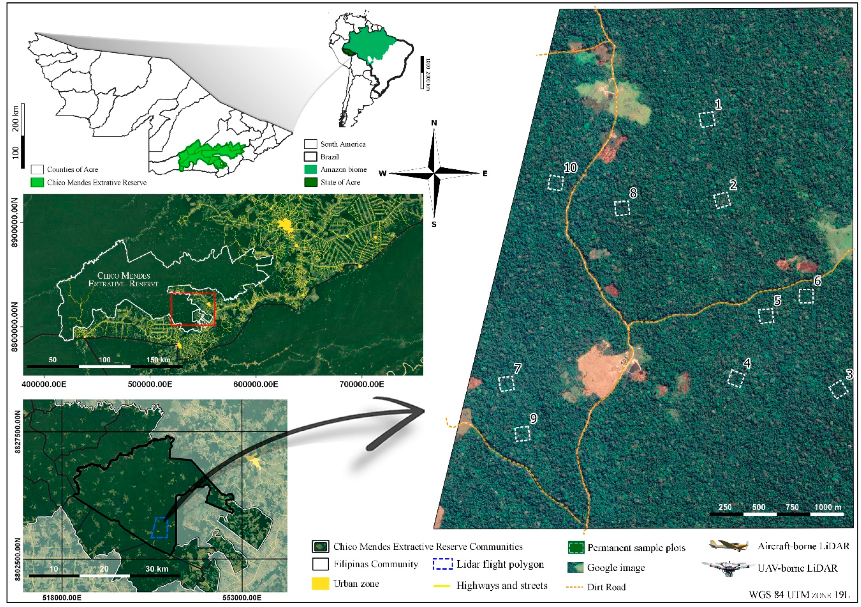
2.1. Study Site

Seringal Filipinas is a small rural community located in the Chico Mendes Extractive Reserve (locally known as Resex Chico Mendes), which is an International Union for Conservation of Nature (IUCN) category VI Protected Area with sustainable use of natural resources, located about 30 km from Brasileia city (Figure 1). The community has little structure for agricultural production and storage, and the primary economic income is from non-timber product extraction. The forest is predominantly open with a transition to a dense forest with a relatively high occurrence of the species Hevea brasiliensis L. and Bertholletia excelsa Bonpl. The climate is classified as Awi (Köppen) with annual precipitation of around 2000 mm and an average temperature of 24 °C, with a dry season between the months of June and September. The area has gentle topography with a maximum elevation range of around 75 m. Because it is contained in an extractive reserve, the forest is typically well conserved with only small areas of secondary forest, pasture, and crops, not exceeding 5% of the total area. However, there have been indications of increased deforestation and selective logging in this area in the last decade [29,30].

2.2. Forest Inventory Plots

A forest inventory was conducted in March 2017. During the inventory, 10 randomly distributed 1 ha (100 × 100 m) permanent sample plots (PSP) were established. The plot boundaries were defined using a handheld compass for azimuths and a measuring tape for length. GPS coordinates of all plot corners were calculated using a differentially corrected GPS with at least 30 minutes of acquisition per point. All woody stems greater than 10 cm in diameter at breast height (DBH) were labeled, measured, and identified. For each tree, oven-dried AGB was estimated with Equation (1), which was developed for a similar forest in the southern Amazon [31]. Ground measurement data were summarized to the plot level for further analysis (Table 1).
AGB = ((DBH)^2.671 × 0.064)/1000

2.3. LiDAR Data Acquisition

Aircraft-borne LiDAR: Discrete return LiDAR data were collected in September 2015 using a Trimble Harrier 68i sensor set to 300 kHz, installed in a Cessna 206 aircraft, flying at 600 m above ground level (AGL) with an average speed of 198 km/h. This system employs full-waveform digitization, and each waveform is then analyzed by Trimble software to identify return peaks, allowing for a theoretically unlimited number of discrete returns per waveform, but typically 3–6. In our landscape dataset (which covers all PSPs), we identified a maximum of 6 returns being present. LiDAR sidelap was 50%, resulting in a point cloud with a minimum (average) density of 5 (14) pts m−2, covering an area of 1000 ha (Table 2). Estimated point absolute spatial accuracy is < 0.25 m horizontal and < 0.15 m vertical (Trimble provided specifications sheet).
UAV-borne LiDAR: Discrete dual return (strongest and last) LiDAR data was collected in August 2017 using the GatorEye Unmanned Flying Laboratory (www.GatorEye.org). The complete sensor suite includes radiometric thermal, high-resolution visual, dual hyperspectral sensors, and LiDAR. The flight platform is a DJI Matrice 600 Pro hexacopter capable of vertical takeoff and landing, with 16 minute flight autonomy for smaller areas and a five km telemetry/control range. In this study, we used only data from the LiDAR sensor. The GatorEye Generation 1 used in this study (the system is now on Gen 3 with a higher-power LiDAR sensor) features a Phoenix Scout integration, including a Velodyne VLP-16 puck lite sensor with dual returns, capable of 600,000 returns per second (Table 2). The system has an L1/L2 dual-frequency Global Navigation Satellite System (GNSS) receiver, and the inertial measurement unit (IMU) is a tactical grade STIM 300. UAV trajectories are obtained through post-process fusion of the IMU and GNSS data in Novatel Inertial Explorer software, differentially corrected to a mobile base station (X900-OPUS) set within 500 m of each launch location. The location of the base station itself was determined using the online Trimble CenterPoint RTX post-processing website. GatorEye flights were conducted at 60 m AGL and an average speed of 30 km/h. LiDAR sidelap was approximately 90%. Point absolute spatial accuracy has been estimated to be <5 cm [32].

2.4. LiDAR Data Processing

The FUSION LiDAR processing package [33] was used for processing the LiDAR all-returns data (first, intermediates, and last returns per pulse) for both GatorEye and aircraft data. LiDAR returns that occurred within each of the ten ground plot polygons were extracted from the acquisition datasets to create an all-returns point cloud file for each plot (Appendix 1). The ground surface elevation (interpolated from the LiDAR digital terrain model) was then subtracted from each return to remove topographic variation within the plot. Descriptive statistics of the LiDAR point cloud vertical structure, using all returns above 1 m, were computed for each plot. The one-meter minimum height above ground was used to reduce noise within the near-ground point cloud caused by low vegetation and imperfections in the ground point filtering.
First, the following layers were produced at a 1 × 1 m spatial resolution: (1) a reference image which serves as a background image for data exploration and display, and which provides sufficient resolution to clearly recognize overstory tree crowns as well as areas of agricultural crops and pastures; (2) digital terrain (DTM) (e.g., elevation-ground), surface (DSM) (top-of-canopy), and canopy height (CHM) models (CHM = DSM − DTM). Second, we computed a suite of forest structural metrics at different spatial resolutions. A list of all computed metrics is provided in Table 3, and a detailed description of each metric is provided in [33]. In overview, the metrics provide information on the vertical distribution of LiDAR points across the forest profile and the shape and heterogeneity of this distribution.
For canopy cover metrics, we used a canopy overstory threshold height of 2 m. Plot-level LiDAR metrics were merged with the summarized field plot data for regression modeling. Raster layers of forest canopy metrics were created using FUSION, following the same methodology used by [7]. All rasters produced were automatically aligned [34]. We then created from the LiDAR point clouds, at a 100 × 100 m resolution, raster layers for the forest structure metrics selected as predictor variables to the AGB models at a raster cell resolution equal to the nominal ground plot size over the entire 1000 ha study area.

2.5. LiDAR Point Cloud, Metrics, and Digital Terrain, Surface, and Height Models Comparison

Comparisons were made between the aircraft- and GatorEye-derived point cloud and filtered ground point density (points m−2) within each PSP polygon (FUSION LiDAR processing package [33]). Pearson correlation analysis was used to determine the linear correlations among metrics from systems (PROC CORR, SAS 9.2). The PROC MIXED (SAS 9.2) procedure was used to test the equivalency of slopes for the adjusted equations between the predicted values. The produced digital terrain models were tested by covariance analysis and the differences between regression parameters (intercept and slope) by means of least squares means test using the SAS 9.2 PROC MIXED.

2.6. Regression Modeling of Aboveground Biomass

Multiple linear regression techniques were used to develop relationships between plot-level LiDAR metrics and field-measured AGB. LiDAR predictor variables were selected using the best subsets approach. The variance inflation factor (VIF) statistics and a Pearson correlation test were used to eliminate highly collinear predictor variables [35,36]. If VIF exceeded 5.0 or ρ above 0.7 for a candidate predictor variable, it was dropped from the regression model. The hypothesis of equal slopes for the adjusted equations between the predicted values for both AGB models was tested by covariance analysis and the differences between parameters by means of least squares means test using the SAS 9.2 PROC MIXED and extrapolated to the entire area covered by LiDAR.

3. Results

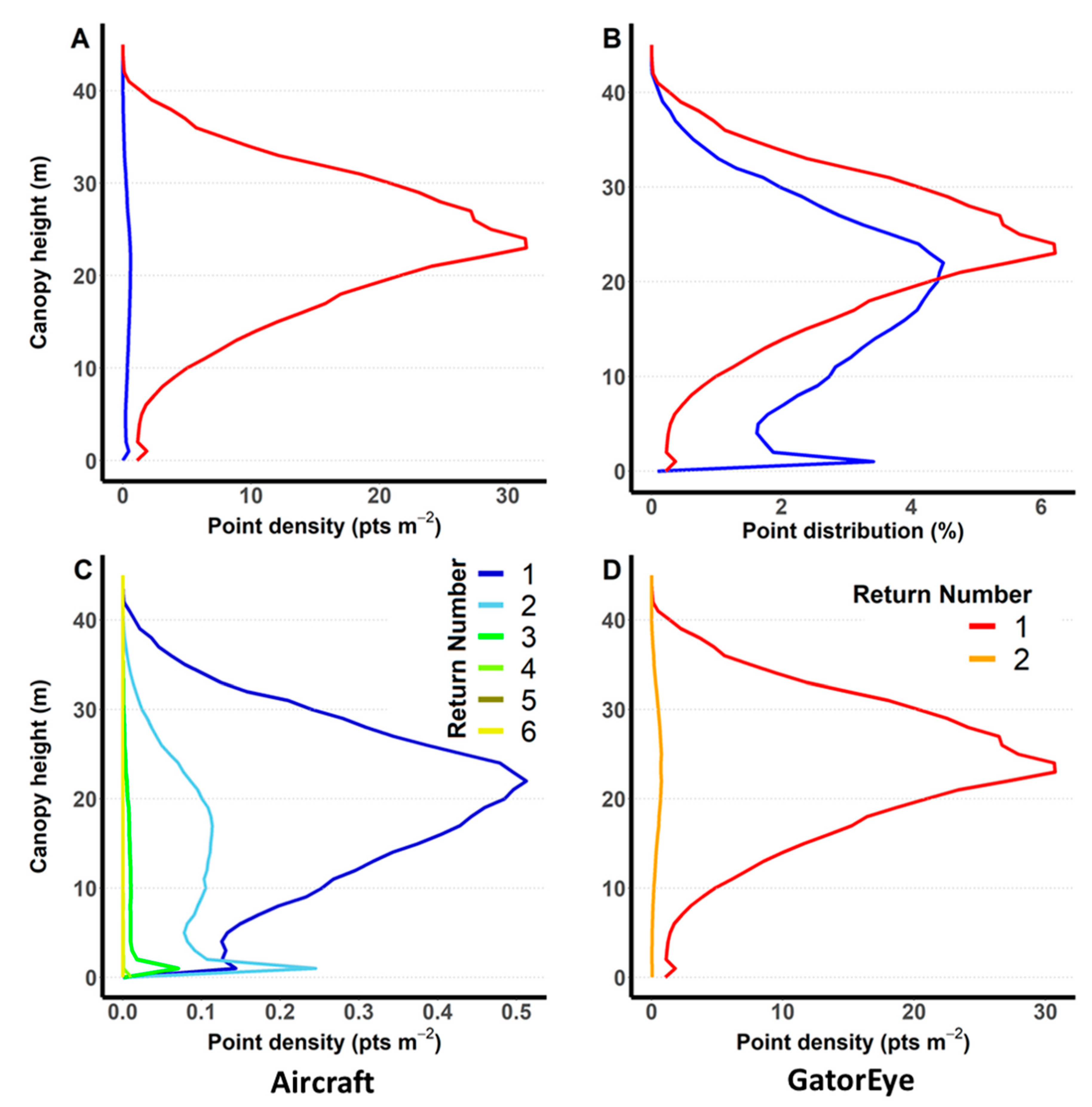
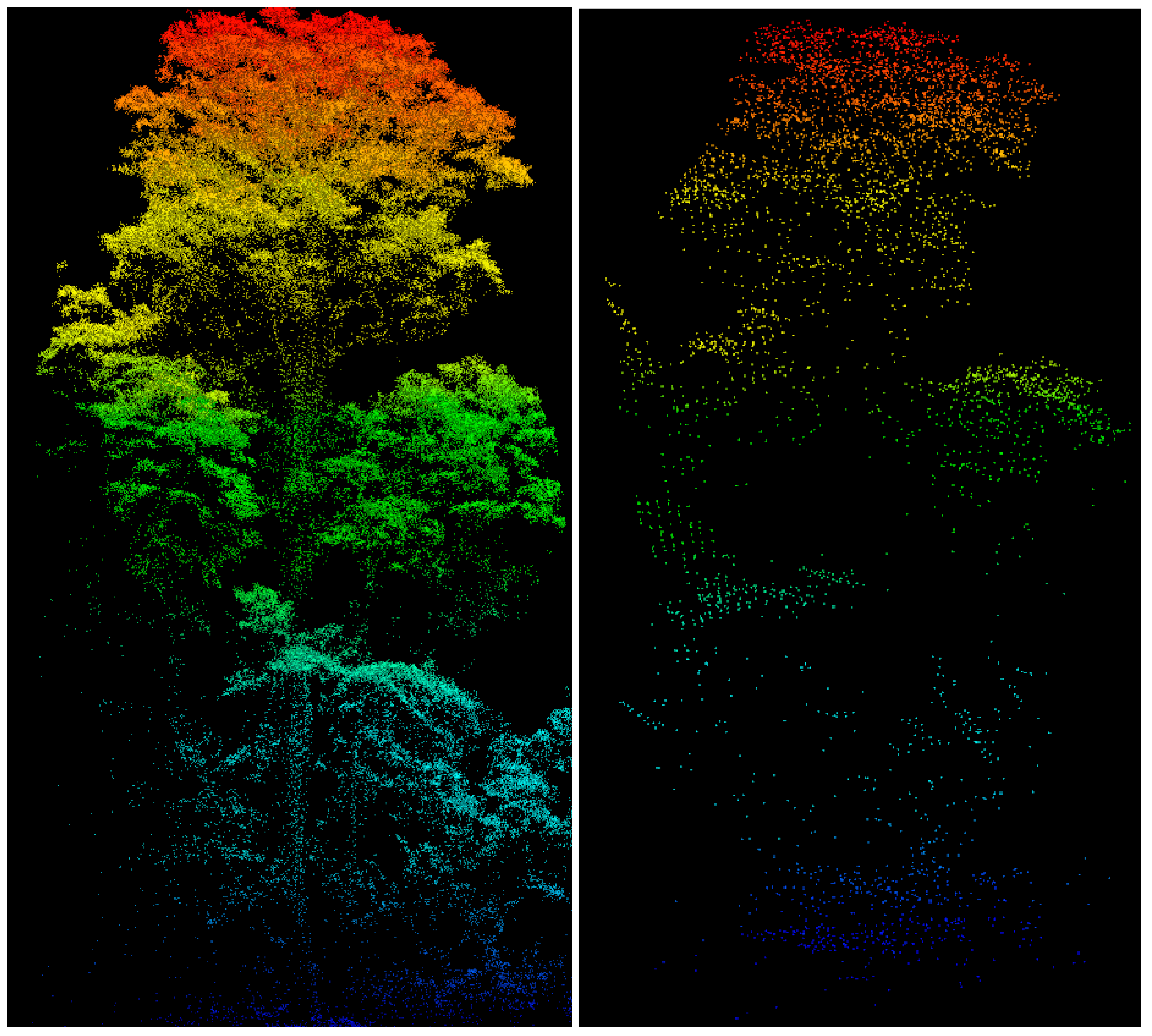
3.1. Comparison of LiDAR Points Clouds

The GatorEye produced about 35 times greater density point clouds than the aircraft system, averaging 381.2 ± 58.2 returns m−2 versus 11.0 ± 1.8 returns m−2, respectively (Table 4, Figure 2A,B). Although in much greater number, the GatorEye LiDAR sensor produces only two returns per pulse (Table 4, Figure 2D), while the aircraft one multiple (4–6 per pulse, Table 4, Figure 2C). The points density profile of the returns reflects the studied area canopy structure with a peak of return numbers around 22 m for both cases. Looking to the point distribution percentage height profile, we observed a higher proportion of aircraft returns below 20 m height produced by the larger LiDAR footprint and the higher number of returns per pulse (Figure 2D). The GatorEye’s higher point cloud number and density resulted in its point clouds producing visibly higher resolution delineation of tree branches and leaf area distribution (Figure 3). The GatorEye’s filtered ground points remained about 1.5 times greater than the aircraft system, with point densities averaging 0.42 ± 0.09 and 0.29 ± 0.09 returns m−2, respectively (Table 4).

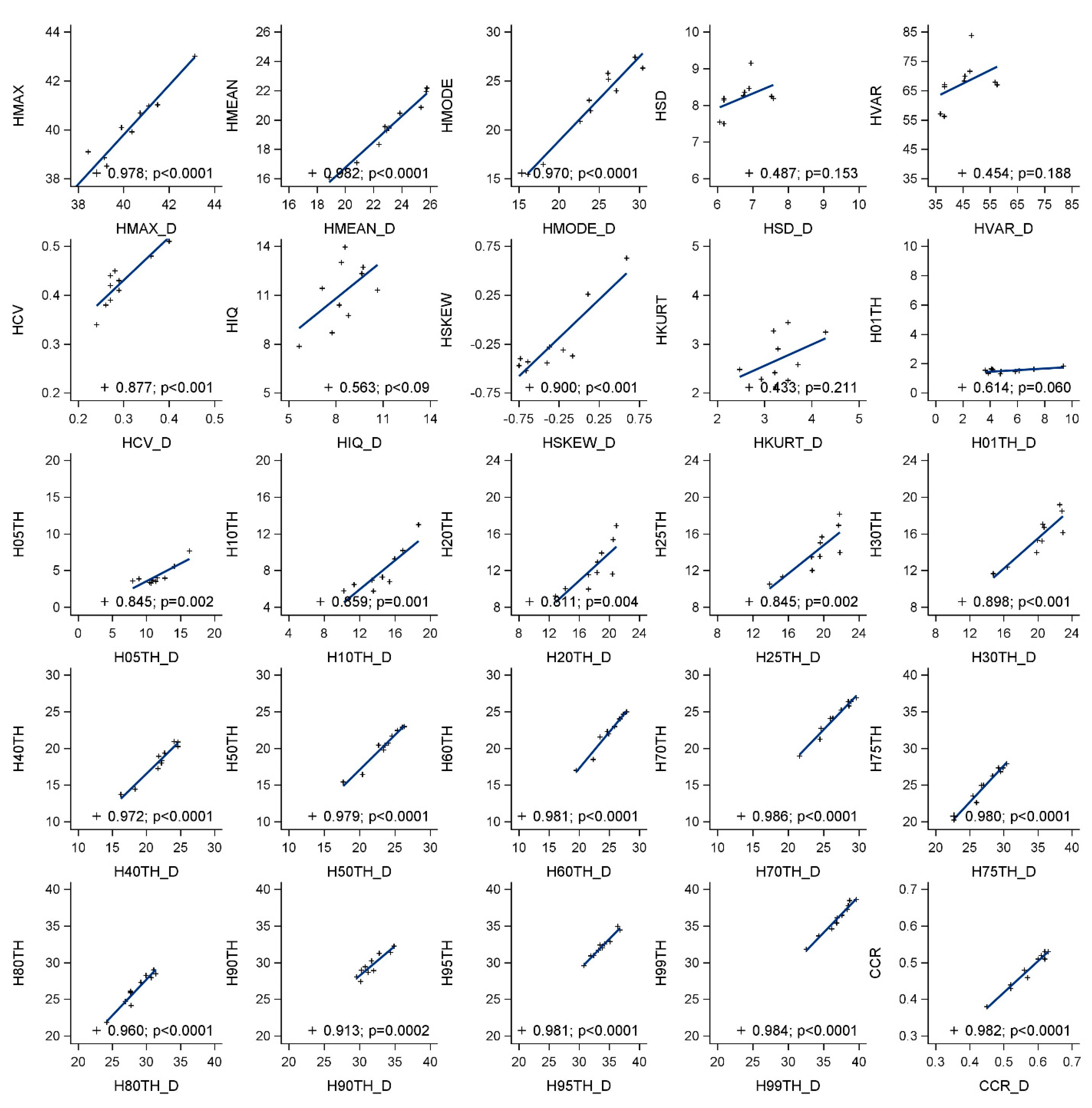
3.2. Comparison of LiDAR Metrics

Plot-scale LiDAR metrics for aircraft and GatorEye systems are presented in Table 5 and Table 6, respectively. Figure 4 shows their statistical comparison and highlights that most metrics were significantly correlated. Metric in the lower height quartiles (H05TH to H20TH) had lower correlations than those in the higher quartiles. Overall, metrics having a poor correlation (p < 0.05; e.g., HSD, HVAR, and HCV) were influenced by point cloud density. Complete tables of Aircraft- and GatorEye-derived LiDAR structural metrics are provided in the Supplementary Materials.

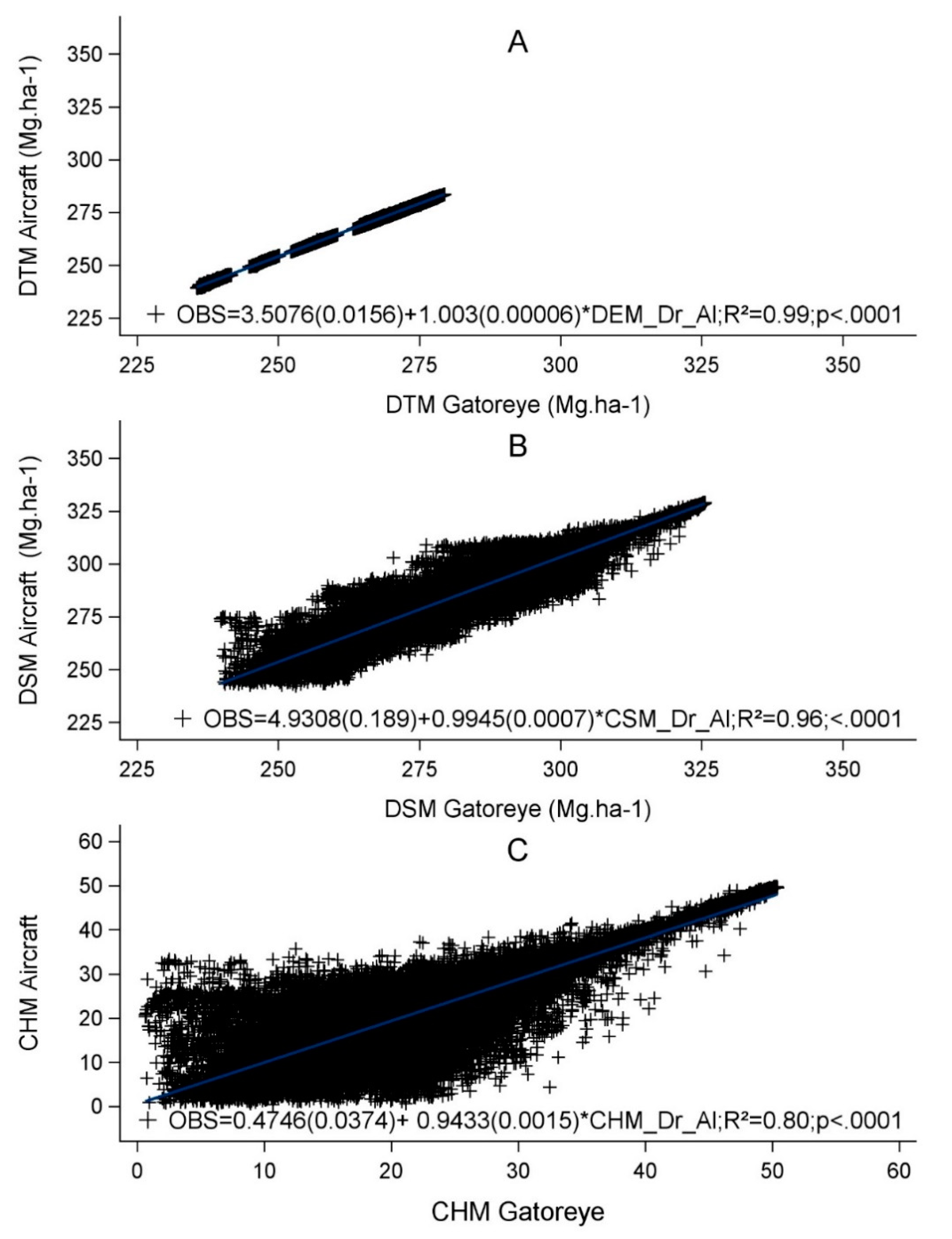
3.3. Comparison of DTM, DSM, and CHM

Figure 4 provides comparisons of the DTM, DSM, and CHM models derived from aircraft and GatorEye system point clouds. The digital terrain models (Figure 5A) were statistically indistinguishable (R2 > 0.99, RMSE = 0.26 m), and the digital surface models (Figure 5B; R2 = 0.96, RMSE = 3.33 m) were significantly and highly positively correlated. The CHM models also present a significant correlation (Figure 5C; R2 = 0.80, RMSE = 3.29 m), but in this case, a height dispersion can be observed, especially at low tree heights, where above 20 m tree heights differences could be identified.

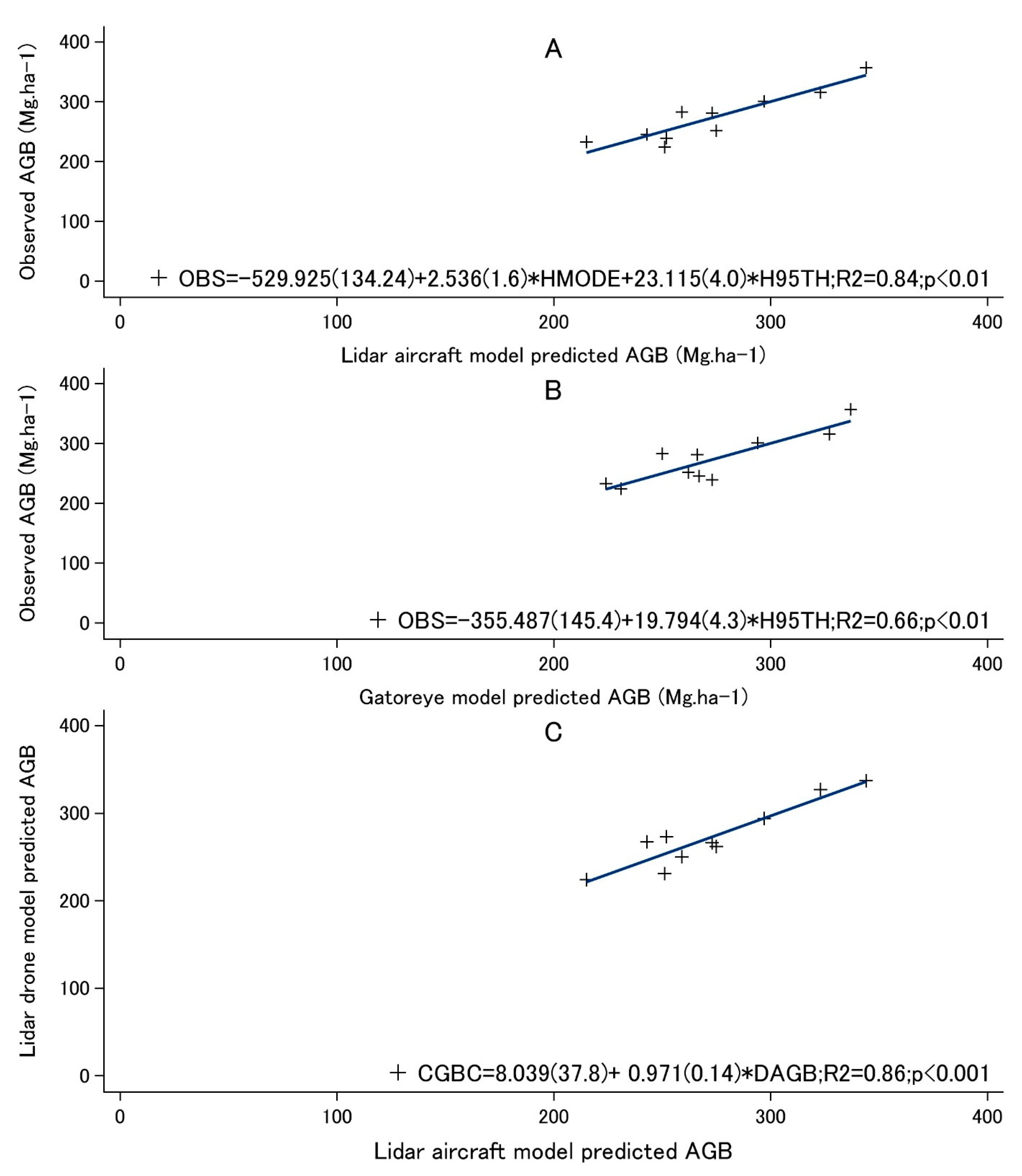
3.4. Regression Modeling of AGB between LiDAR and Field Data

Table 5 summarizes the models evaluated for AGB produced by the two systems. The metrics for the height mode and 95th percentile height above ground for aircraft-borne LiDAR provided the most parsimonious multivariate model (Adj. R2 = 0.79, RMSE = 19.3 Mg·ha−1). For the GatorEye, the best fit was obtained with the 90th percentile height above ground (Adj. R2 = 0.65, RMSE = 24.8 Mg·ha−1). Other models were generated, but all of them presented VIF above 5 or Pearson correlation test > 0.7 and were discarded.
Figure 6 displays the predicted and observed AGB values for each plot for models from the aircraft (6A) and GatorEye systems (6B) and their inter-comparison (C). The predicted values from the models were highly correlated (R2 = 0.90, RMSE = 13.23 Mg·ha−1). Table 6 summarizes the AGB estimates by the models for each PSP. The mean AGB estimates by the aircraft and GatorEye systems were 273.1 ± 12.2 and 273.1 ± 11.1 Mg·ha−1, respectively. Although variations can be observed between modeled and field derived estimates, the mean for the plots by all approaches was close to the same (273 Mg·ha−1).

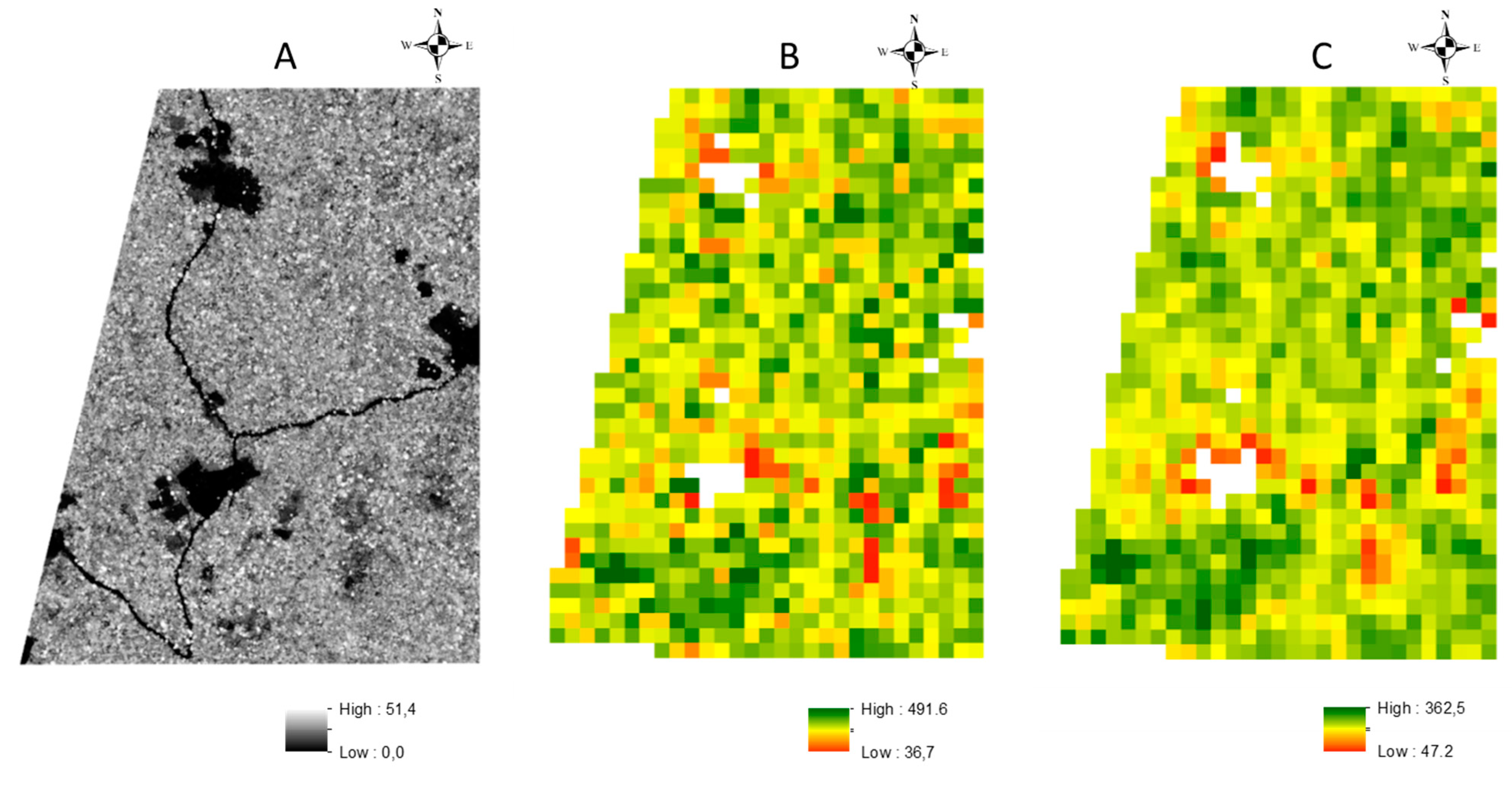
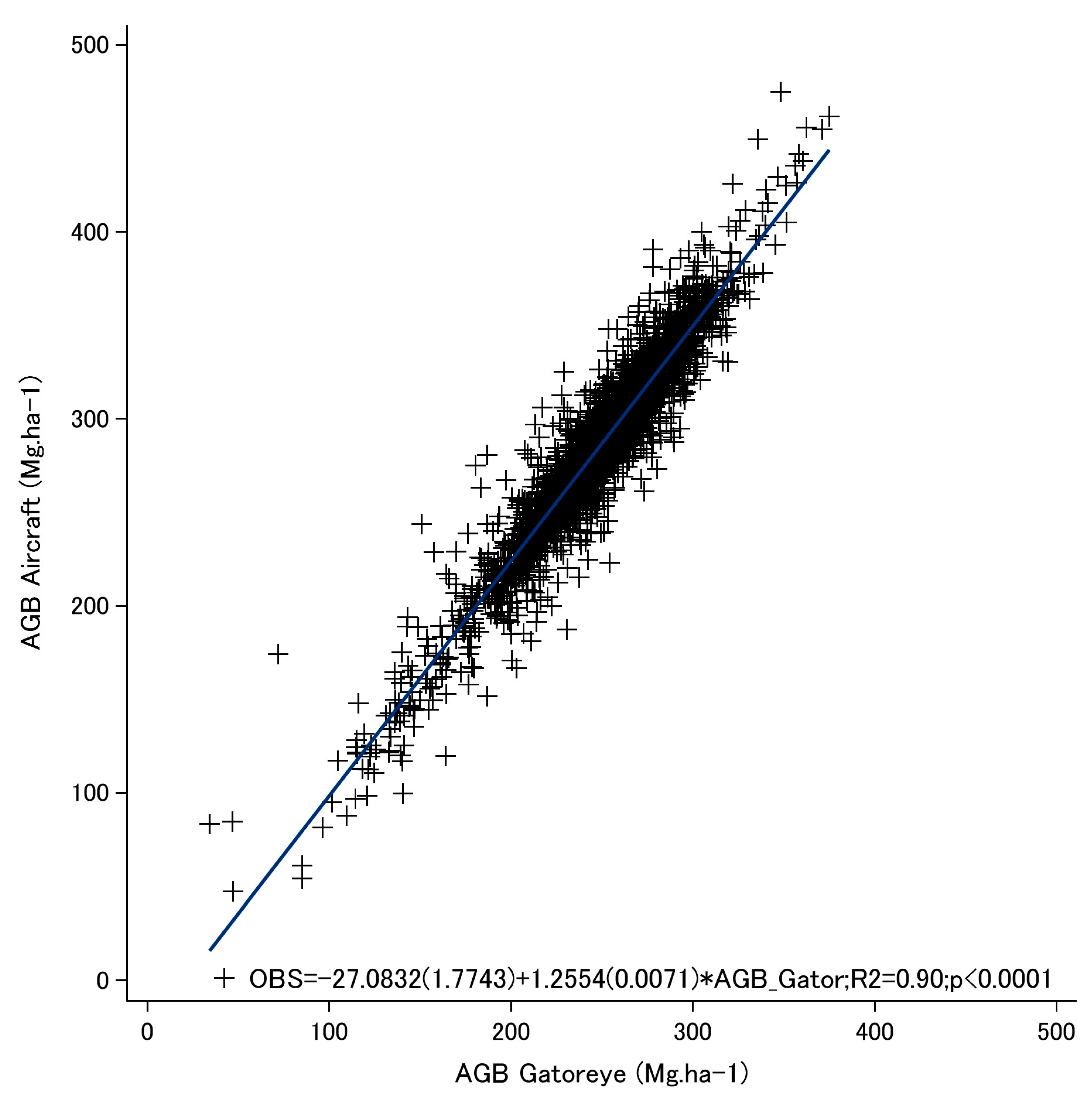
3.5. Landscape-scale Analysis

Figure 7 illustrates an extrapolation of the aircraft-system AGB models to the full 1000 ha landscape at a plot-scale 100 × 100 m resolution. We can observe non-forest areas occupied by agriculture crops, pastures, and secondary forests (7A). These areas were mapped as no data (blank cells in Figure 7B,C) as their AGB values were out of the range of the model input data. The predicted AGB across the entire landscape for the aircraft and GatorEye predictive equations averaged 247.7 ± 37.2 Mg·ha−1 (B) and 283.9 ± 61.6 Mg·ha−1 (C), respectively, and they were highly correlated: R2 = 0.90, RMSE = 14.2, N = 3.330 (Figure 8). However, the AGB values estimated by the two models do not correspond 1:1; in other words, intercept and slope coefficients values are statistically different from 0 and 1, respectively (Figure 8).

4. Discussion

Our study demonstrates the potential of UAV-borne LiDAR to assess the structure and biomass of tropical forests in the Amazon. To our knowledge, this is the first study to compare aircraft- and UAV-borne LiDAR AGB predictions for tropical forests. The plots did not suffer significant natural or anthropogenic disturbances during the two-year interval (2015–2017) between the aircraft and GatorEye flights. As, during this time, only limited natural changes in the forest canopy occurred, we were able to robustly compare vegetation metrics and models produced by the two systems, similar to as if they had happened synchronously [37].
The GatorEye sensor pulse frequency was only twice the Harrier 68i Trimble, but, in part due to having 16 lasers versus the one used in the Harrier system, it produced a point cloud almost 35 times denser. The main differences between the point clouds generated by these sensors were due to the GatorEye lower flight height and speed (60 m AGL at 12 m/s) when compared with the aircraft (600 m at 55 m/s), and due to the number of lasers. Low-altitude flight at relatively slow speeds can produce point densities much higher than traditional aircraft LiDAR approaches [38]. The dense point cloud generated by GatorEye in this study was similar to or higher than that of other UAV-borne LiDAR systems [28,39], which allowed the identification of individual tree and branch structure with results similar, in the overstory, to terrestrial laser scanners. That allows a broader use of these data for applications such as individual canopy tree detection, stem segmentation, tree height, and estimation of understory leaf area index [21,24]. The differences in point cloud density were possibly responsible for the main differences observed among the extracted LiDAR metrics. Even when the density of the points is not as high as in this study, they can significantly improve CHM-based metrics derived from vegetation in both temperate and tropical forests [40].
Some UAV-borne LiDAR sensors are capable of producing multi-return per pulse (e.g., RIEGL VUX series); however, the GatorEye’s Velodyne VLP-16 sensor returns the strongest and last returns. When we compared the ground-filtered clouds of both sensors, we observed that even when flying at a higher altitude and speed, the Harrier 68i was capable of producing up to five useful returns per pulse. The second and particularly third pulse echoes mostly exist beneath trees [22]; thus analyzing the Harrier 68i ground filtered point cloud, we observe more second and third returns than first. The cloud density of the ground returns of the GatorEye’s cloud was still higher than that from the aircraft system but had a higher standard deviation in the number of ground returns per area, indicating the GatorEye ground points were not as uniformly distributed across the ground as the returns produced by the aircraft system. We attribute this difference to the GatorEye acquiring very dense point in areas of lower leaf area index (LAI), with more limited returns in areas of dense coverage, while the aircraft-system more fully penetrated across the entire forest floor.
The differences highlighted above did not affect the correlation of the high-resolution (1 × 1 m) digital terrain models (DTM) produced by both systems within the PSPs. Typically, at high resolutions, the relatively low-density point clouds of both systems would force estimation of ground location and forest structure through statistical interpolation approaches [14]. However, we found an almost total agreement between the DTMs from both systems, indicating that the ground returns from both systems were sufficient to fully and accurately represent the forest ground surface—a critical aspect for post-process work such as AGB calculation.
Different from the DTM, although highly correlated, the much higher GatorEye point cloud density, and the time interval between the flights, did produce some noticeable differences between the DSM and CHM models. Changes observed in the forest structure, through natural tree falls and growth canopy trees as well as within previously existing gap areas in the PSP, produced height differences. Thus, some negative height differences (CHM 2017–CHM2015) can be attributed to tree- and branch-fall gap creation and positive height differences made by pioneer species rapidly growing in the previously existing forest gaps. However, due to the large dispersion observed between CHM models, other factors such as i. crown delineation inconsistencies created by individual tree growth or absence of returns to computed tree height in a cell (in particular for the lower density aircraft data); ii. differences in flight and LiDAR sensors specifications (e.g., with a much higher number of returns per area, the GatorEye data resulted in a higher number of heights in the cells, generating a better chance to identify the highest part of the treetop); iii. phenological phases differences (e.g., flowering or leaves fall); and iv. crown movement by wind [14] also contributed to the observed differences between models.
The AGB model produced by the aircraft system presented a higher R2 value and lower RMSE. In similar studies, despite technical differences in the LiDAR data acquisition, the AGB models produced by UAV-borne LiDAR (e.g., [41]) had similar accuracy to those produced by aircraft systems (e.g., [8,12]). Other factors, such as the quality of fieldwork on the establishment, measurement, and geolocation of the ground plots, also can strongly affect the accuracy of the models. Still, in this study, the models were developed from the same PSP data and geolocation.
All AGB models produced presented high accuracy, and the uncertainty at 1 ha resolution was lower or comparable with values previously reported in other tropical forests for both aircraft and UAV-based LiDAR systems [5,13,41]. The inclusion of more LiDAR independent variables produced models with higher R2 statistics. The use of more than two independent variables to compose a LiDAR AGB model is considered acceptable (e.g., [42]); however, to avoid highly collinear LiDAR metrics that would limit the model’s predictive usefulness over the range of forest structure condition in the study site [7], we only accepted models with VIF below 5 and Pearson correlation test below 0.7. In our study, the best model to the aircraft was a combination of two LiDAR metrics representing the forest higher stratum (Elev P95) and the elevation mode (Elev mode) [43] and to GatorEye an univariate model based only in the 90th percentile above ground height. Correlation coefficients above 0.8 are not typical in tropical forests, but we found a study [37] where, in similar conditions, the authors found a very high accuracy in a model built with three independent variables. In our study, we built models for both GatorEye and Aircraft with Adj. R2 > 0.9 with acceptable VIF (below 5), but we discarded these models because they present Pearson correlation > 0.7.
The AGB models produced by both systems were highly correlated; however, there was no 1:1 statistical correspondence. Therefore, both systems proved to be equally efficient for estimating ABG, but the models of both systems were not statistically equal. Although the average biomass estimated at the landscape scale was very similar, the reduced statistical correspondence was likely due to the canopy structure changing during the two-year difference between LiDAR data collections. We believe that studies using data collected in the same period may achieve the statistical correspondence match between the models from the two systems.
One current use of the AGB models produced by LiDAR is through the use of satellite images to upscale AGB estimates to a regional scale. Usually, when large LiDAR samples are available, a first upscale is performed from the field plot scale to LiDAR sampled area [44,45]. Here, we tested the possibility to upscale the AGB model produced by GatorEye. AGB LiDAR models can be, when functioning correctly, generalized [46] or applied in different regions [42]. In our extrapolation of both models to the entire area covered by the 2015 LiDAR flight, the AGB maps produced presented a surprisingly high correlation, as both models used the same LiDAR metrics as independent variables, and these metrics were unaffected by the difference in cloud point density (see Figure 3). When the same procedure was performed with the GatorEye univariate regression model, although the model correlation was still high, there was a tendency for the model to slightly underestimate AGB values.

5. Conclusions

The aircraft and GatorEye systems produced highly correlated LiDAR products, including DTMs, DSMs and CHMs, forest structural metrics, and AGB models. In general, the main differences were a result of the GatorEye providing a much higher point cloud density, resulting from a lower and slower flight pattern with a higher return per time period and a complete 360-degree horizontal and 30-degrees vertical scan angle field-of-view (FOV) sensor incorporating 16x the number of lasers. A small number of natural disturbances that occurred during the two years between flights was visible by comparing the DSMs. Ground returns of the GatorEye were still higher but less so than the overall point cloud due to the aircraft system’s multiple returns. The LiDAR AGB models produced by both systems presented similar accuracy and AGB estimation at the plot level, as well as when upscaled across the entire 1000 ha landscape scale flown by the aircraft system in 2015.
Our results highlight the advantages of and recommend the use of UAV-borne LiDAR sensors as an effective approach for monitoring forest AGB stock dynamics in areas where previously only aircraft-borne LiDAR could be considered. We also highlight new possibilities feasible with these uniquely high-density point clouds, including multi-temporal 3D monitoring and analyses of detailed crown structure and interior forest leaf area density distribution, which can be indicators of forest structure and AGB stocks and dynamics.

Supplementary Materials

The following are available online at https://www.mdpi.com/2072-4292/12/11/1754/s1, Table S1.1: Aircraft system derived LiDAR forest structural metrics for the PSP, Table S1.2: GatorEye system derived LiDAR forest structural metrics for the PSP.

Author Contributions

Conceptualization, M.V.N.d., E.N.B., A.M.A.Z., D.R.A.A., F.S.A., R.A.M., E.O.F., M.O.-d.-C., and L.C.O.; methodology, M.V.N.d., E.N.B., A.M.A.Z., D.R.A.A., and L.C.O.; software, M.V.N.d., E.N.B., A.M.A.Z., D.R.A.A., G.A.P., and L.C.O.; validation, M.V.N.d., E.N.B., A.M.A.Z., and D.R.A.A.; analysis, M.V.N.d., E.N.B., A.M.A.Z., and D.R.A.A.; investigation, M.V.N.d., E.N.B., A.M.A.Z., and D.R.A.A.; resources, M.V.N.d., E.N.B., A.M.A.Z., D.R.A.A., and L.C.O.; data curation, M.V.N.d., E.N.B., A.M.A.Z., and L.C.O.; writing—original draft preparation, M.V.N.d., E.N.B., D.R.A.A., D.A.P., and L.C.O.; writing—review and editing, M.V.N.d., E.N.B., A.M.A.Z., D.R.A.A., D.A.P., C.A.S., M.E.F., F.S.A., G.A.P., R.A.M., E.O.F., B.W., L.A.d.C.J., L.J., R.W.A., P.H.S.B., M.O.-d.-C., and L.C.O.; visualization, D.A.P., M.V.N.d., E.N.B., G.A.P., A.M.A.Z., and L.C.O.; supervision, M.V.N.d., and E.N.B.; project administration, M.V.N.d., E.N.B., M.O.-d.-C., F.S.A., and R.A.M.; funding acquisition, M.V.N.d., E.N.B., A.M.A.Z., R.A.M., F.S.A., and M.O.-d.-C.; All authors have read and agreed to the published version of the manuscript.

Acknowledgments

We thank the Acre State government, BID, and CAPES for the support of the inventory plots establishment and aircraft LiDAR flight. We thank the Embrapa Acre parabotanic team for their support during fieldwork. We thank the McIntire-Stennis USDA funding program for financial support assisting the development of the GatorEye Unmanned Flying Laboratory. We thank the donors to the WWF Brazil program who helped fund the field logistics related to the GatorEye data collection in the Resex Chico Mendes. We thank the School of Forest Resources and Conservation at the University of Florida for financial support for the development of the GatorEye system and for supporting work by Broadbent and Almeyda Zambrano during the field campaign and in subsequent post-processing and analysis. We thank the families in the Chico Mendes Extractive Reserve for providing us access to their properties where the PSPs are situated and for providing excellent field support, great meals, and good conversation during our field campaigns. D. Almeida was supported by the São Paulo Research Foundation (#2018/21338-3 and #2019/14697-0). Finally, we thank the Fototerra team for the 2015 LiDAR datum adjustment.

Conflicts of Interest

The authors declare no conflict of interest.

References

  1. Beets, P.N.; Brandon, A.M.; Goulding, C.J.; Kimberley, M.O.; Paul, T.S.H.; Searles, N. The inventory of carbon stock in New Zealand’s post-1989 planted forest for reporting under the Kyoto protocol. For. Ecol. Manag. 2011, 262, 1119–1130. [Google Scholar] [CrossRef]
  2. Bottalico, F.; Chirici, G.; Giannini, R.; Mele, S.; Mura, M.; Puxeddu, M.; McRoberts, R.E.; Valbuena, R.; Travaglini, D. Modeling Mediterranean forest structure using airborne laser scanning data. Int. J. Appl. Earth Obs. Geoinf. 2017, 57, 145–153. [Google Scholar] [CrossRef]
  3. Liu, K.; Shen, X.; Cao, L.; Wang, G.; Cao, F. Estimating forest structural attributes using UAV-LiDAR data in Ginkgo plantations. ISPRS J. Photogramm. Remote Sens. 2018, 146, 465–482. [Google Scholar] [CrossRef]
  4. Meyer, V.; Saatchi, S.; Clark, D.B.; Keller, M.; Vincent, G.; Ferraz, A.; Espírito-Santo, F.; d’Oliveira, M.V.N.; Kaki, D.; Chave, J. Canopy area of large trees explains aboveground biomass variations across nine neotropical forest landscapes. Biogeosciences 2018, 15, 3377–3390. [Google Scholar] [CrossRef] [Green Version]
  5. Zhao, K.; Suarez, J.K.; Garcia, M.; Hu, T.; Wange, C.; Londo, A. Utility of multitemporal LiDAR for forest and carbon monitoring: Tree growth, biomass dynamics, and carbon flux. Remote Sen. Environ. 2018, 204, 883–897. [Google Scholar] [CrossRef]
  6. Meyer, V.; Saatchi, S.S.; Chave, J.; Dalling, J.W.; Bohlman, S.; Fricker, G.A.; Robinson, C.; Neumann, M.; Hubbell, S. Detecting tropical forest biomass dynamics from repeated airborne LiDAR measurements. Biogeosciences 2013, 10, 5421–5438. [Google Scholar] [CrossRef] [Green Version]
  7. D’Oliveira, M.V.N.; Reutebuch, S.E.; McGaughey, R.J.; Andersen, H. Estimating forest biomass and identifying low-intensity logging areas using airborne scanning LiDAR in Antimary State Forest, Acre State, Western Brazilian Amazon. Remote Sen. Environ. 2012, 124, 479–491. [Google Scholar] [CrossRef]
  8. Ellis, P.; Griscom, B.; Walker, W.; Gonçalvez, F.; Cormier, T. Mapping selective logging impacts in Borneo with GPS and airborne LiDAR. For. Ecol. Manag. 2016, 365, 184–196. [Google Scholar] [CrossRef] [Green Version]
  9. Melendy, L.; Hagen, S.C.; Sullivan, F.B.; Pearson, T.R.H.; Walker, S.M.; Ellis, P.; Kustiyo; Sambodo, A.K.; Roswintiarti, O.; Hanson, M.A. Automated method for measuring the extent of selective logging damage with airborne LiDAR data. ISPRS J. Photogramm. Remote Sens. 2018, 139, 228–240. [Google Scholar] [CrossRef]
  10. Griscom, B.M.; Ellis, P.W.; Burivalova, Z.; Halperin, J.; Marthinus, D.; Runting, R.K.; Ruslandi; Shochh, D.; Putz, F.E. Reduced-impact logging in Borneo to minimize carbon emissions and impacts on sensitive habitats while maintaining timber yields. For. Ecol. Manag. 2019, 438, 176–185. [Google Scholar] [CrossRef]
  11. Papa, D.A.; de Almeida, D.R.A.; Silva, C.A.; Figueiredo, E.O.; Stark, S.C.; Valbuena, R.; d’Oliveira, M.V.N. Evaluating tropical forest classification and field sampling stratification from LiDAR to reduce effort and enable landscape monitoring. For. Ecol. Manag. 2020, 457, 117634. [Google Scholar] [CrossRef]
  12. Andersen, H.E.; Reutebuch, S.E.; McGaughey, R.J.; d’Oliveira, M.V.N.; Keller, M. Monitoring selective logging in western Amazonia with repeat LIDAR flights. Remote Sens. Environ. 2014, 151, 157–165. [Google Scholar] [CrossRef] [Green Version]
  13. Réjou-Méchain, M.; Tymena, B.; Blanc, L.; Fauset, S.; Feldpausch, T.R.; Monteagudo, A.; Phillips, O.L.; Richard, H.; Chave, J. Using repeated small-footprint LiDAR acquisitions to infer spatial and temporal variations of a high-biomass Neotropical forest. Remote Sens. Environ. 2015, 169, 93–101. [Google Scholar] [CrossRef]
  14. Brede, B.; Lau, A.; Bartholomeus, H.M.; Kooistra, L. Comparing RIEGL RiCOPTER UAV LiDAR derived canopy height and DBH with terrestrial LiDAR. Sensors 2017, 17, 2371. [Google Scholar] [CrossRef] [PubMed]
  15. Colomina, I.; Molina, P. Unmanned aerial systems for photogrammetry and remote sensing: A review. ISPRS J. Photogramm. Remote Sens. 2014, 92, 79–97. [Google Scholar] [CrossRef] [Green Version]
  16. Paneque-Gálvez, J.; McCall, M.K.; Napoletano, M.M.; Wich, S.A.; Koh, L.P. Small drones for community-based forest monitoring: An assessment of their feasibility and potential in tropical areas. Forests 2014, 5, 1481–1507. [Google Scholar] [CrossRef] [Green Version]
  17. Tang, L.; Shao, G. Drone remote sensing for forestry research and practices. J. For. Res. 2015, 26, 791–797. [Google Scholar] [CrossRef]
  18. Messinger, M.; Asner, G.P.; Silman, M. Rapid Assessments of Amazon forest structure and biomass using Small Unmanned Aerial Systems. Remote Sens. 2016, 8, 615. [Google Scholar] [CrossRef] [Green Version]
  19. Zahawi, R.A.; Dandois, J.P.; Holl, K.D.; Nadwodny, D.; Reid, J.L.; Ellis, E.C. Using lightweight unmanned aerial vehicles to monitor tropical forest recovery. Biol. Conserv. 2015, 186, 287–295. [Google Scholar] [CrossRef] [Green Version]
  20. Thiel, C.; Schmullius, C. Comparison of UAV photograph-based and airborne LiDAR-based point clouds over forest from a forestry application perspective. Int. J. Remote Sens. 2017, 38, 2411–2426. [Google Scholar] [CrossRef]
  21. Almeida, D.R.A.; Stark, S.C.; Shao, G.; Schietti, J.; Nelson, B.W.; Silva, C.A.; Brancalion, P.H.S. Optimizing the remote detection of tropical rainforest structure with airborne LiDAR: Leaf area profile sensitivity to pulse density and spatial sampling. Remote Sens 2019, 11, 92. [Google Scholar] [CrossRef] [Green Version]
  22. Lin, Y.; Hyyppä, J.; Jaakkola, A.A. Mini-UAV-Borne LIDAR for fine-scale mapping. IEEE Geosci. Remote Sens. Lett. 2011, 8, 426–430. [Google Scholar] [CrossRef]
  23. Wallace, L.; Lucier, A.; Watson, C.; Turner, D. Development of a UAV-LiDAR system with application to forest inventory. Remote Sens. 2012, 4, 1519–1543. [Google Scholar] [CrossRef] [Green Version]
  24. Corte, A.P.D.; Rex, F.E.; Almeida, D.R.A.D.; Sanquetta, C.R.; Silva, C.A.; Moura, M.M.; Wilkinson, B.; Zambrano, A.M.A.; Neto, C.; Veras, H.F.; et al. Measuring individual tree diameter and height using GatorEye High-Density UAV-Lidar in an integrated crop-livestock-forest system. Remote Sens. 2020, 12, 863. [Google Scholar] [CrossRef] [Green Version]
  25. Figueiredo, E.O.; d’Oliveira, M.V.N.; Braz, E.M.; Papa, D.A.; Fearnside, P.M. Lidar-based estimation of bole biomass for precision management of an Amazonian forest: Comparisons of ground-based and remotely sensed estimates. Remote Sens. Environ. 2016, 187, 281–293. [Google Scholar] [CrossRef] [Green Version]
  26. Almeida, D.R.A.; Broadbent, E.N.; Zambrano, A.M.A.; Wilkinson, B.E.; Ferreira, M.E.; Chazdon, R.; Melia, P.; Gorgen, E.B.; Silva, C.A.; Stark, S.C.; et al. Monitoring the structure of forest restoration plantations with a drone-LiDAR system. Int. J. Appl. Earth Obs. Geoinf. 2019, 79, 192–198. [Google Scholar] [CrossRef]
  27. Barbour, T.E.; Sassaman, K.E.; Zambrano, A.M.A.; Broadbent, E.N.; Wilkinson, B.; Kanaski, R. Rare pre-Columbian settlement on the Florida Gulf Coast revealed through high-resolution drone LiDAR. Proc. Natl. Acad. Sci. USA 2019, 116, 23493–23498. [Google Scholar] [CrossRef]
  28. Yin, D.; Wang, L. Individual mangrove tree measurement using UAV-based LiDAR data: Possibilities and challenges. Remote Sens. Environ. 2019, 223, 34–49. [Google Scholar] [CrossRef]
  29. Vadjunec, J.M.; Rocheleau, D. Beyond forest cover: Land use and biodiversity in rubber trail forests of the Chico Mendes Extractive Reserve. Ecol. Soc. 2009, 14, 29. Available online: http://www.ecologyandsociety.org/vol14/iss2/art29/ (accessed on 24 January 2020). [CrossRef] [Green Version]
  30. Duchelle, A.E.; Guariguata, M.R.; Less, G.; Albornoz, M.A.; Chavez, A.; Melo, T. Evaluating the opportunities and limitations to multiple use of Brazil nuts and timber in Western Amazonia. For. Ecol. Manag. 2012, 268, 39–48. [Google Scholar] [CrossRef]
  31. De Melo, A.W.F. Alometria de Árvores e Biomassa Florestal na Amazônia Sul-Ocidental. Ph.D. Thesis, Instituto Nacional de Pesquisas da Amazônia, Manaus, Brazil, 2017. [Google Scholar]
  32. Wilkinson, B.; Lassiter, H.A.; Abd-Elrahman, A.; Carthy, R.R.; Ifju, P.; Broadbent, E.; Grimes, N. Geometric Targets for UAS Lidar. Remote Sens. 2019, 11, 3019. [Google Scholar] [CrossRef] [Green Version]
  33. McGaughey, R.J. FUSION/LDV: Software for LIDAR Data Analysis and Visualization; United States Department of Agriculture, Forest Service, Pacific Northwest Research Station: Washington, DC, USA, 2018; 154p. [Google Scholar]
  34. Environmental Systems Research Institute (ESRI). ArcMap software, ArcGIS Release 10.4; Environmental Systems Research Institute (ESRI): Redlands, CA, USA, 2019. [Google Scholar]
  35. Fox, J.; Monette, G. Generalized collinearity diagnostics. J. Am. Stat. Assoc. 1992, 87, 178–183. [Google Scholar] [CrossRef]
  36. Dou, J.; Yunus, A.P.; Merghadi, A.; Shirzadi, A.; Nguyen, H.; Hussain, Y.; Avtar, R.; Chen, Y.L.; Pham, B.T.; Yamagishi, H. Different sampling strategies for predicting landslide susceptibilities are deemedless consequential with deep learning. Sci. Total Environ. 2020, 720, 137320. [Google Scholar] [CrossRef] [PubMed]
  37. Bater, C.W.; Wulder, M.A.; Coops, N.C.; Nelson, R.F.; Hilker, T.; Nasset, E. Stability of Sample-Based Scanning-LiDAR-Derived vegetation metrics for forest monitoring. IEEE Trans. Geosci. Remote Sens. 2011, 49, 2385–2392. [Google Scholar] [CrossRef]
  38. Mohan, M.; Silva, C.A.; Klauberg, C.; Jat, P.; Catts, G.; Cardil, A.; Hudak, A.T.; Dia, M. Individual tree detection from Unmanned Aerial Vehicle (UAV) derived canopy height model in an open canopy Mixed Conifer Forest. Forests 2017, 8, 340. [Google Scholar] [CrossRef] [Green Version]
  39. Guerra-Hernández, J.; Cosenza, D.N.; Estraviz, L.C.; Silva, R.M.; Tomé, M.; Díaz-Varela, R.A.; González-Ferreiro, E. Comparison of ALS- and UAV(SfM)-derived high density point clouds for individual tree detection in Eucalyptus plantations. Int. J. Remote Sens. 2018, 39, 5211–5235. [Google Scholar] [CrossRef]
  40. Garcia1, M.; Saatchi, S.; Ferraz, A.; Silva, C.A.; Ustin, S.; Koltunov, A.; Balzter, H. Impact of data model and point density on aboveground forest biomass estimation from airborne LiDAR. Carbon Balance Manag. 2017, 12, 4. [Google Scholar] [CrossRef] [Green Version]
  41. Wang, D.; Wana, B.; Liuc, J.; Sue, Y.; Guoe, Q.; Qiuf, P.; Wu, X. Estimating aboveground biomass of the mangrove forests on northeast Hainan Island in China using an upscaling method from field plots, UAVLiDAR data and Sentinel-2 imagery. Int. J. Appl. Earth Obs. Geoinf. 2020, 85, 101986. [Google Scholar] [CrossRef]
  42. Drake, J.B.; Dubayaha, R.O.; Clark, D.B.; Knox, R.G.; Blair, J.B.; Hofton, M.A.; Chazdon, R.L.; Weishampel, J.F.; Prince, S.D. Estimation of tropical forest structural characteristics using large-footprint LiDAR. Remote Sens. Environ. 2002, 79, 305–319. [Google Scholar] [CrossRef]
  43. Mura, M.; McRoberts, R.E.; Chirici, G.; Marchetti, M. Estimating and mapping forest structural diversity using airborne laser scanning data. Remote Sens. Environ. 2015, 170, 133–142. [Google Scholar] [CrossRef]
  44. Asner, G.P.; Mascaro, J.; Anderson, C.; Knapp, D.E.; Martin, R.E.; Kennedy-Bowdoin, T.; van Breugel, B.; Davies, S.; Hall, J.S.; Muller-Landau, H.C.; et al. High-fidelity national carbon mapping for resource management and REDD+. Carbon Balance Manag. 2013, 8, 7. [Google Scholar] [CrossRef] [PubMed] [Green Version]
  45. Saatchi, S.; Xu, A.; Meyer, V.; Ferraz, Y.; Shapiro, A.; Witteger, L.; Lee, M.; Tshibasu, E.; Banks, N. Carbon Map of DRC: A Summary Report of UCLA Institute of Environment & Sustainability; UCLA: Los Angeles, CA, USA, 2017; 62p. [Google Scholar]
  46. Asner, G.P.; Mascaro, J.; Muller-Landau, H.C.; Vieilledent, G.; Vaudry, R.; Rasamoelina, M.; Hall, J.S.; Van Breugel, M. A universal airborne LiDAR approach for tropical forest carbon mapping. Oecologia 2011, 168, 1147–1160. [Google Scholar] [CrossRef] [PubMed]
Figure 1. Map of Acre State and its location in South America (top left), the Resex Chico Mendes (middle and bottom left), the BR 317, and the surrounding urban areas (Brasileia and Epitaciolândia cities). The black polygon in the bottom left map is the Seringal Filipinas, and the blue polygon is the 1000 ha area covered by Light Detection And Ranging (LiDAR) flight in 2015. The Google map on the right represents the area covered by the 2015 LiDAR flight and the 15 established permanent sample plots (PSPs).
Remotesensing 12 01754 g001
Figure 2. (A,B) GatorEye (red) and Aircraft (blue) LiDAR point density (pts m−2) and distribution (% per 1 m vertical zone) vertical profiles. (C) Vertical profile of point density for all returns for aircraft (1–6) and (D) for GatorEye (2).
Remotesensing 12 01754 g002
Figure 3. Example LiDAR point clouds of a canopy tree located in Permanent Sample Plot (PSP) 14 produced by the GatorEye (A) and Aircraft (B) systems, highlighting the increased crown, branch, and trunk resolution of the GatorEye system.
Remotesensing 12 01754 g003
Figure 4. Comparison of the metrics produced by LiDAR sensors on the aircraft and GatorEye systems. Metrics ending with “D” were those calculated using GatorEye LiDAR (a.k.a, drone).
Remotesensing 12 01754 g004
Figure 5. Comparison of the digital terrain model ((A)—DTM), digital surface model ((B)—DSM), and digital height model ((C)—DHM/canopy height model (CHM)) produced by aircraft and GatorEye systems. Numbers in parentheses are the standard errors for each coefficient.
Remotesensing 12 01754 g005
Figure 6. Predicted versus observed ground plot values for aboveground biomass (Mg·ha−1) for models produced by the (A) aircraft system and (B) GatorEye system, and (C) their comparison. Numbers in parentheses are the standard errors for each coefficient.
Remotesensing 12 01754 g006
Figure 7. (A) Canopy height model (CHM) at 1 × 1 m resolution, showing forest canopy gaps and anthropogenic features, including roads, crops, pastures, and secondary forests, and aboveground biomass (AGB; Mg ha−1) estimates from the (B) aircraft and (C) GatorEye predictive equations, at a 100 × 100 m plot-scale resolution. Blank cells in the AGB models are non-forest areas. All maps are based on the aircraft-derived LiDAR data acquired in 2015.
Remotesensing 12 01754 g007
Figure 8. Predicted AGB across the entire landscape for the aircraft and GatorEye predictive models correlation: Aircraft: −529.761 + (2.536 × HMODE) + (23.115 × H95TH), R2 = 0.79, RMSE = 19.3 and GatorEye: −355.4877 + (19.794 × H90TH), R2 = 0.65, RMSE = 24.87) and GatorEye: −418.01 + (7.2625 × HMODE) + ( 24.2363 × H95TH) + (−535.1370 × CRR), R2 = 0.77, RMSE = 20.16. Numbers in parentheses are the standard errors for each coefficient.
Remotesensing 12 01754 g008
Table 1. Plot identification (ID), number of trees and aboveground biomass (AGB Mg·ha−1) to the permanent sample plots established at the Seringal Filipinas in the Resex Chico Mendes.
Plot IDNumber of TreesAGB Mg·ha−1
1543252.17
2498224.44
3596239.16
4576283.38
5628280.81
6667233.07
7548244.82
8579300.85
9519315.95
10590356.50
Mean558.33293.99
SE15.2810.66
Table 2. Aircraft and GatorEye LiDAR acquisition and product specifications.
SpecificationAircraftGatorEye
Lidar sensorHarrier 68i Trimble (300 kHz)Velodyne VLP-16 Puck Lite (600 kHz)
Flying altitude (AGL)600 m60 m
Laser number116
Beam divergence0.25 mrad (1/e)3.0 mrad (1/e)
Scan angle: horizontal field of view±15 degrees off-nadirFull 360 degrees off-nadir
Vertical field of view±1±15 degrees
Swath sidelap50%80%
Approximate pulse density>4 m2>500 m2
Datum (Horizontal)WGS 84WGS-84
ProjectionUTM, Zone 19SUTM, Zone 19S
Datum (Vertical)WGS 84ITRF 2014
Pulse diameter at target15–30 cm2–8 cm
Horizontal accuracy50–75 cm2–5 cm
Vertical accuracy15–50 cm2–5 cm
Lidar raw point cloud formatLAS format with classified ground points identifiedLAS format with classified ground points identified
Table 3. LiDAR-derived forest structure metrics.
Metric AbbreviationMetric Description
HMAXMaximum height above ground
HMEANMean height above ground
HMEDIANMedian height above ground
HMODEMode height above ground
HSDStandard deviation of height above ground
HVARVariance of height above ground
HCVCoefficient of variation of height above ground
HIQInterquartile distance of height above ground
HSKEWSkewness of height above ground
HKURTHeight kurtosis of height above ground
H.% (e.g., H05TH–H99TH)Percentiles of height above the ground (AGL): 5th, 10th, 20th, 25th, 30th, 40th, 50th, 60th, 70th, 75th, 80th, 90th, 95th, 99th
CCRCanopy relief rate (CCR)
Table 4. Summary statistics for aircraft- and GatorEye-system-derived LiDAR point clouds extracted from the permanent sample plots.
GatorEye—all returns
Return number123456Total
Total49,166,9751,406,827000050,573,802
Maximum return density461.3
Average return density381.2
Standard deviation of return density58.2
GatorEye—filtered ground returns
Return number123456Total
Total51,5713383 54,954
Maximum return density 0.60
Average return density 0.42
Standard deviation0.09
Aircraft—all returns
Return number123456Total
Total1,068,490333,99042,54321313911,447,194
Maximum return density14.2
Average return density11.0
Standard deviation of return density1.8
Aircraft—filtered ground returns
Return number123456Total
Total544320,817769763516134,609
Maximum return density0.43
Average return density0.27
Standard deviation of return density0.09
Table 5. Regression models for aboveground biomass (AGB; Mg·ha−1) relating field-estimated AGB and forest metrics calculated with aircraft and GatorEye LiDAR data.
LiDARRegression ModelFAdj. R2RMSE
Aircraft
Model−529.761 + (2.536 × HMODE) + (23.115 × H95TH)18.030.7919.3
GatorEye
Model−355.4877 + (19.794 × H90TH)18.000.6524.8
Table 6. Aboveground biomass estimates (AGB; Mg·ha−1) produced by the LiDAR models and field measurements for each Permanent Sample Plot (PSP).
PSPFieldAircraftGatorEye
1252.2275.20261.6694
2224.4250.58253.9894
3239.2252.37277.7421
4283.4258.72241.4598
5280.8273.08271.7643
6233.1214.78229.2271
7244.8243.30243.0037
8300.9297.36293.7159
9316.0322.73324.7331
10356.5343.69333.8977
Mean273.1273.18273.12
SE12.712.2411.12

