Assessing the Accuracy and Feasibility of Using Close-Range Photogrammetry to Measure Channelized Erosion with a Consumer-Grade Camera


Abstract
1. Introduction
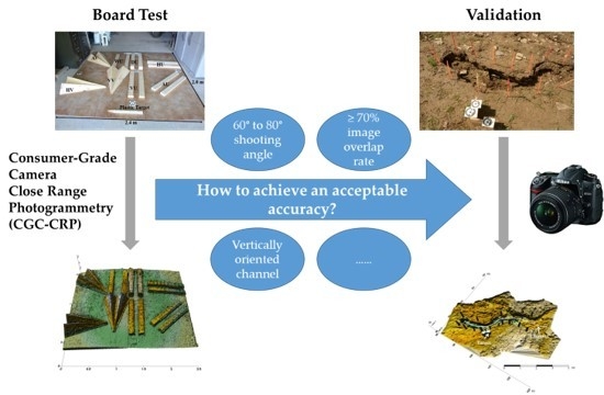
- To estimate the accuracies of the CGC-CRP method under different settings on detecting erosion channels and similar morphological features.
- To assess the applicability of the CGC-CRP method under scenarios with various spatial, temporal, and resource constraints.
2. Materials and Methods
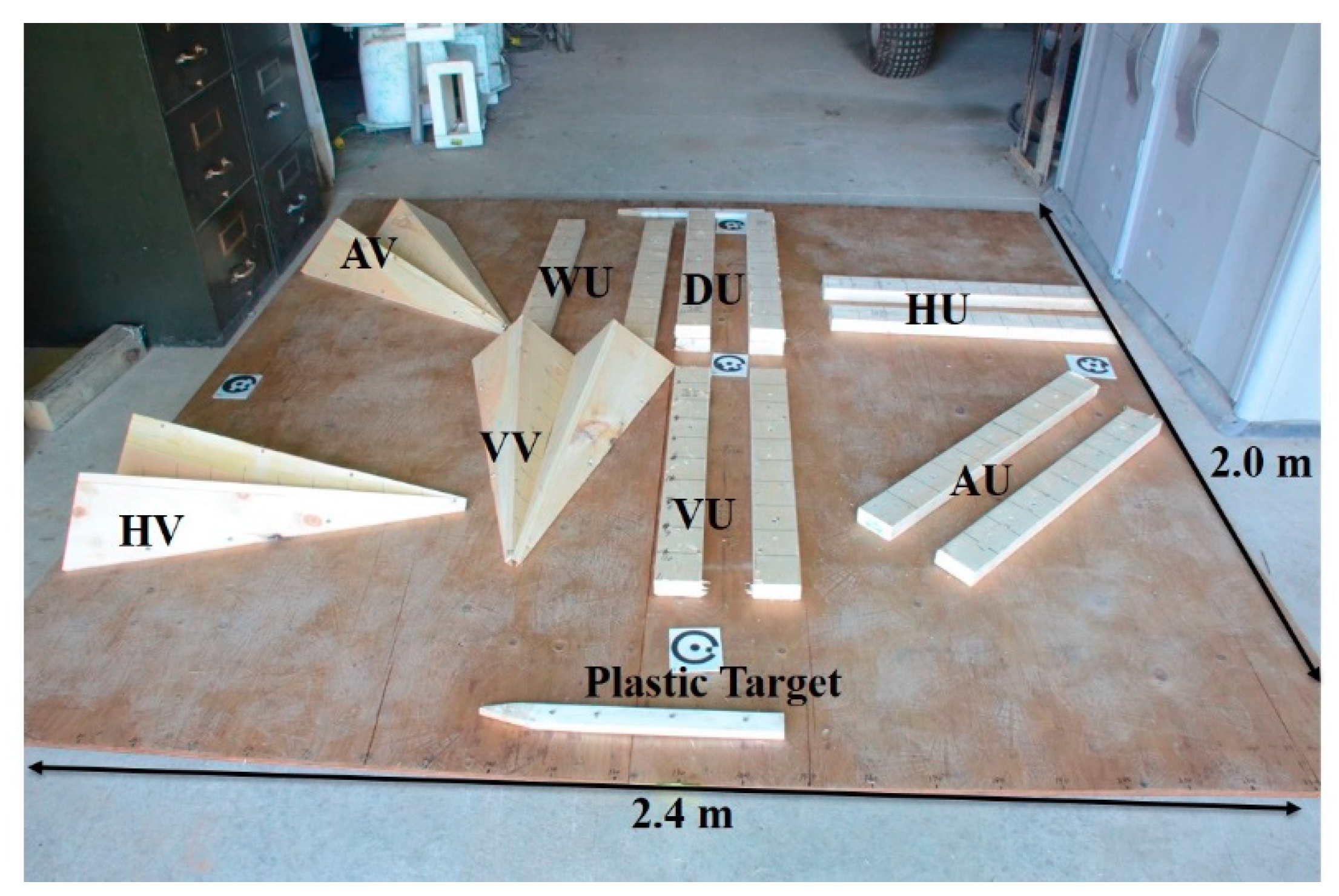
2.1. Study Surfaces
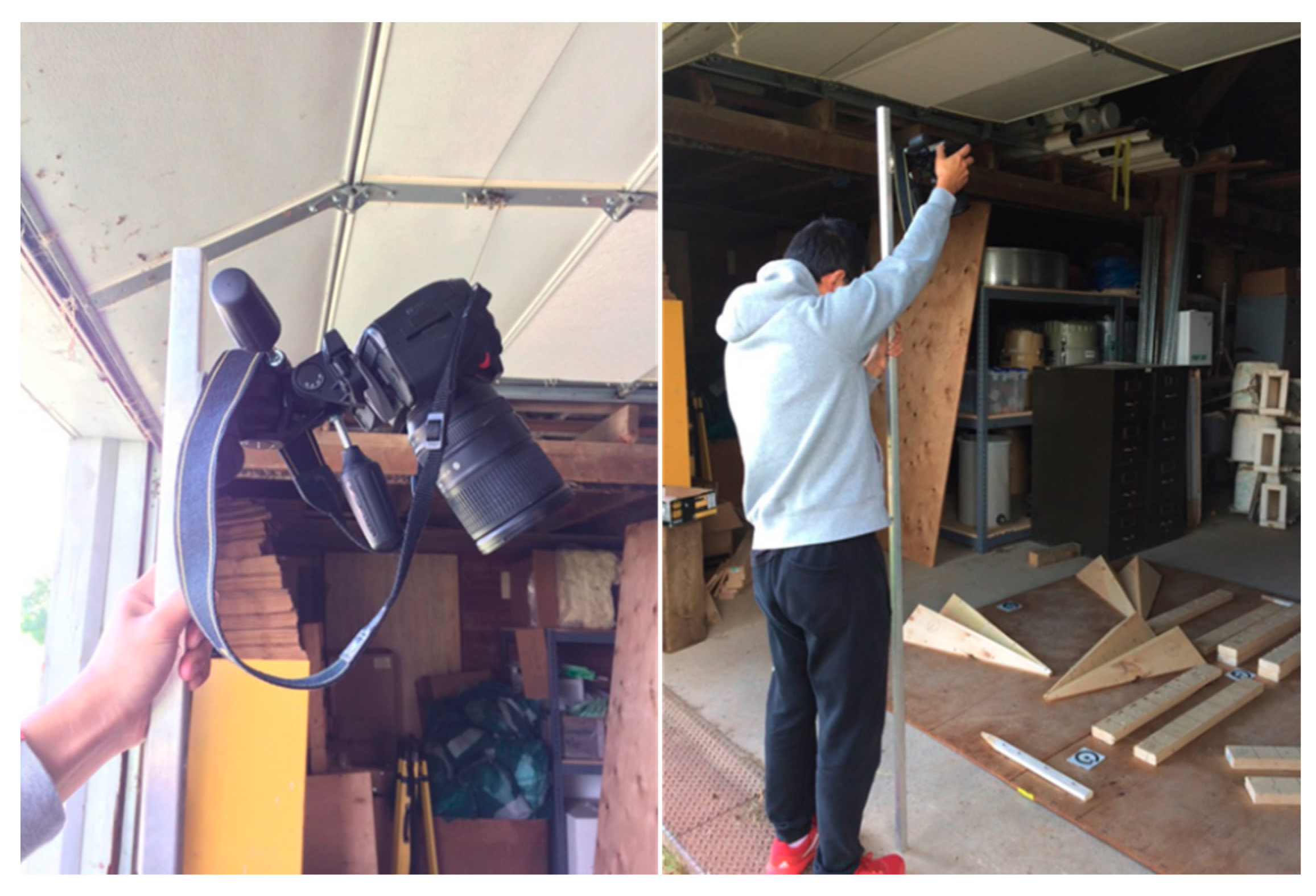
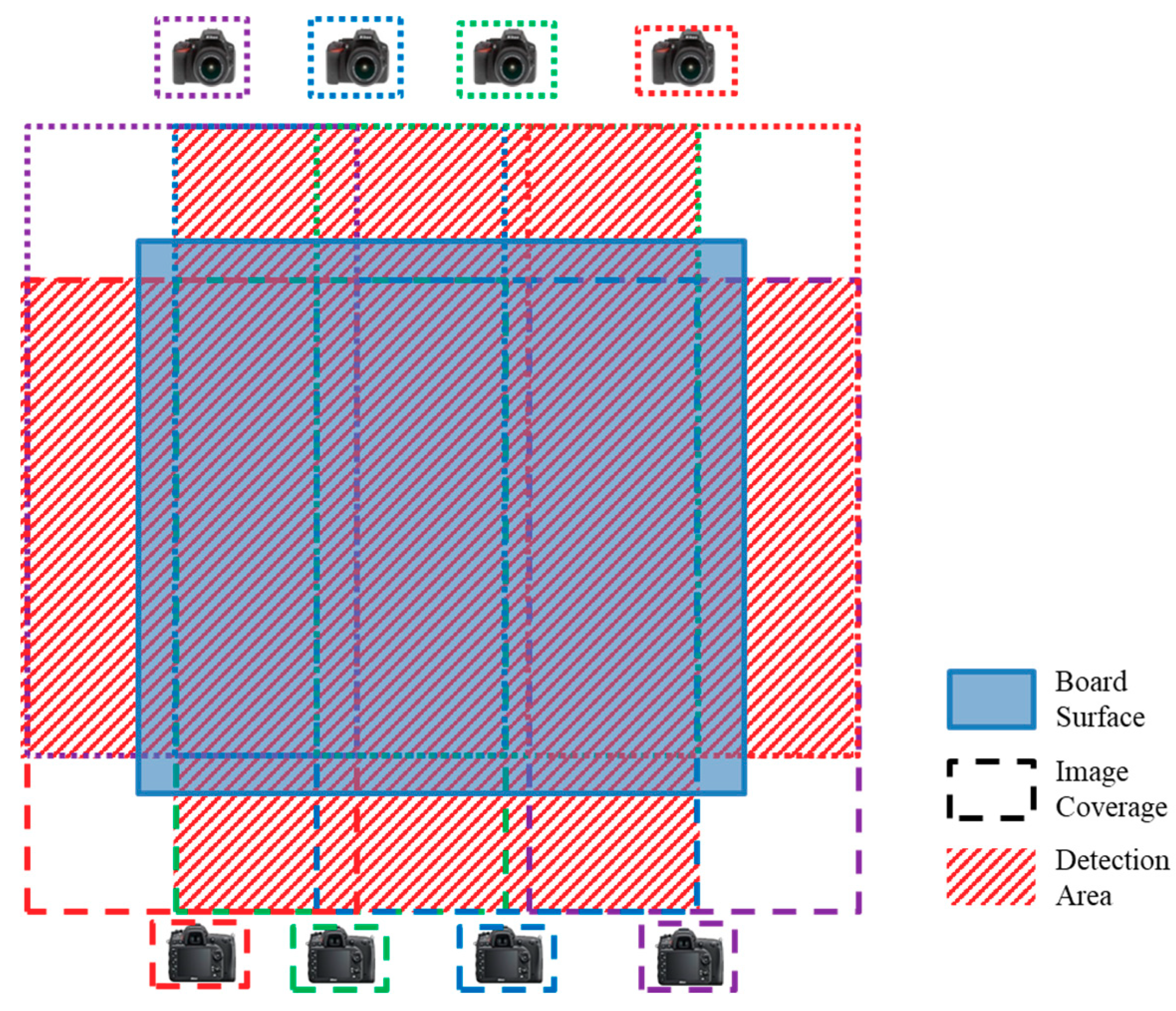
2.2. Data Collection
2.2.1. Manual Measurement
2.2.2. Consumer-Grade Camera Based Photogrammetry (CGC-CRP)
2.3. Data Extraction and Analysis
2.4. Applicability Measures
3. Results
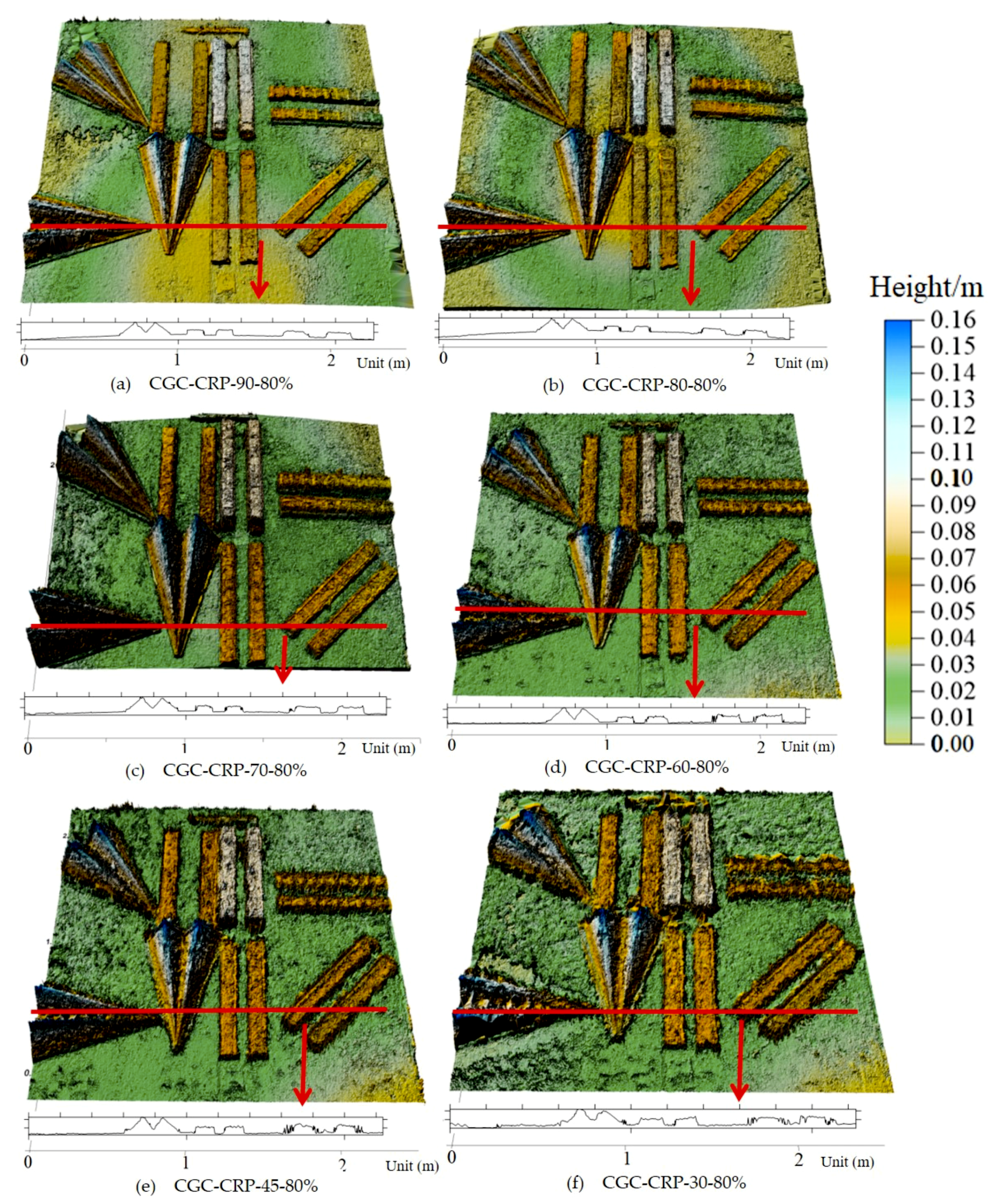
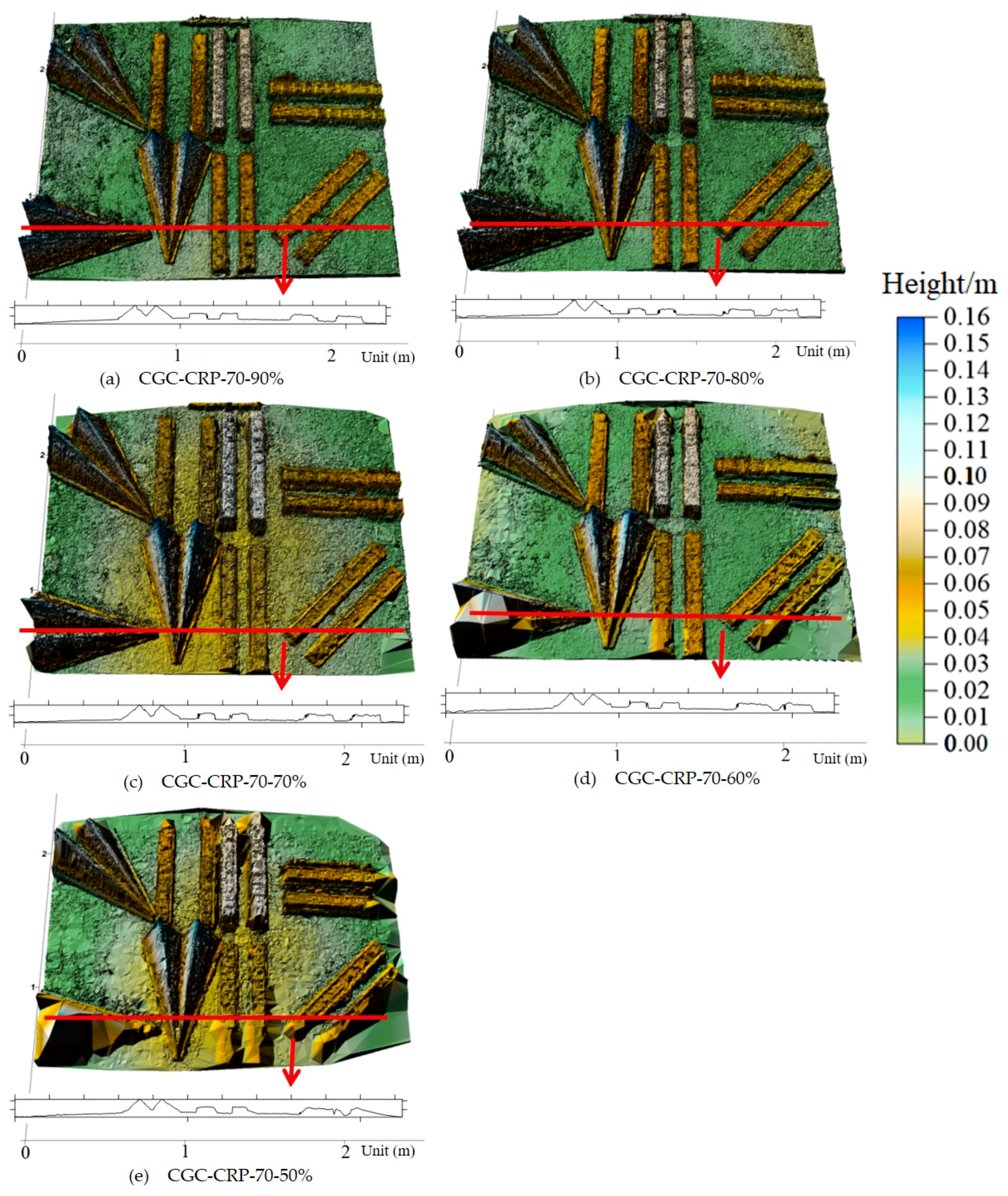
3.1. Artificial Surface
3.1.1. Visual Observation of the DEMs
3.1.2. U-Channels
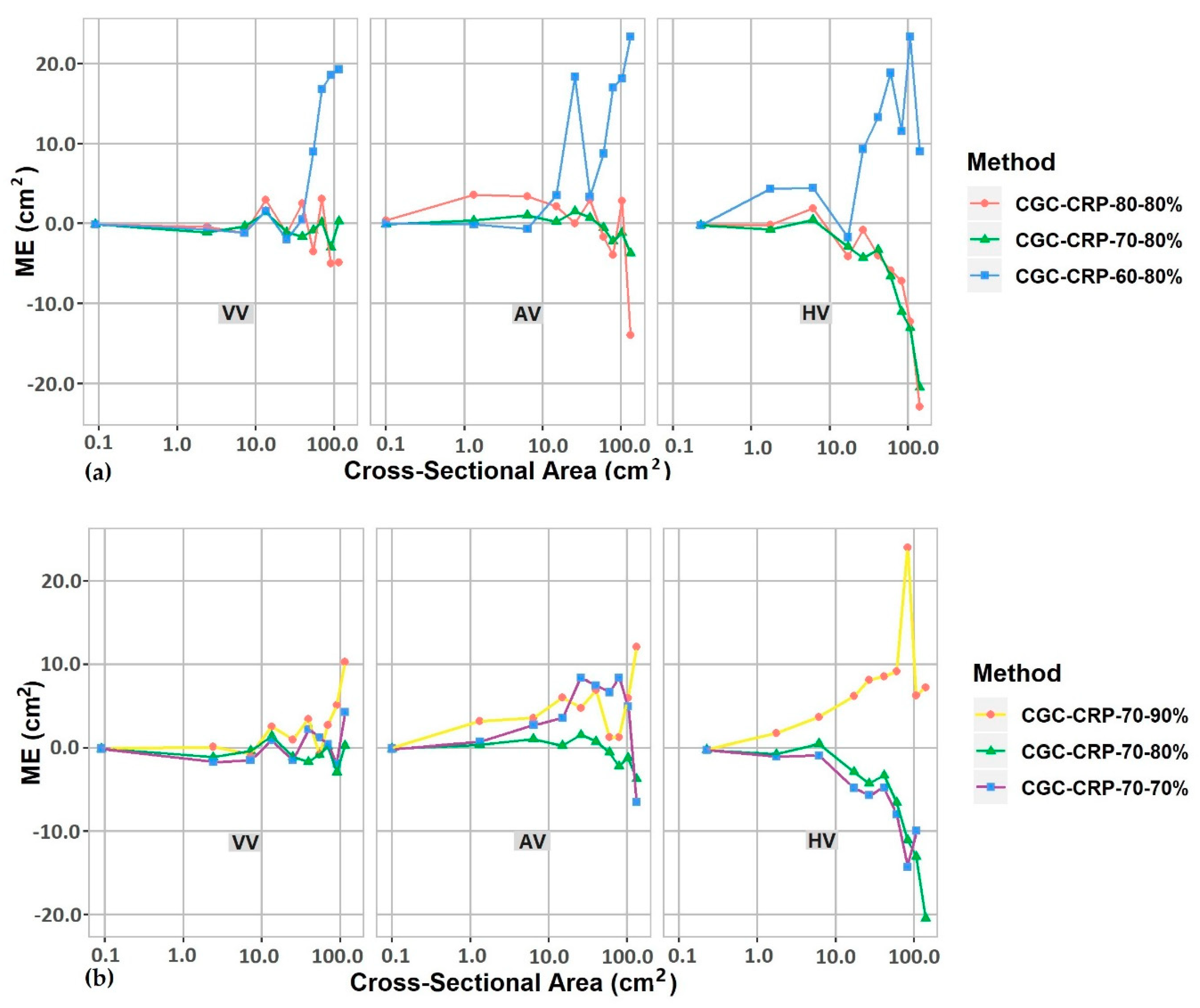
3.1.3. V-Channels
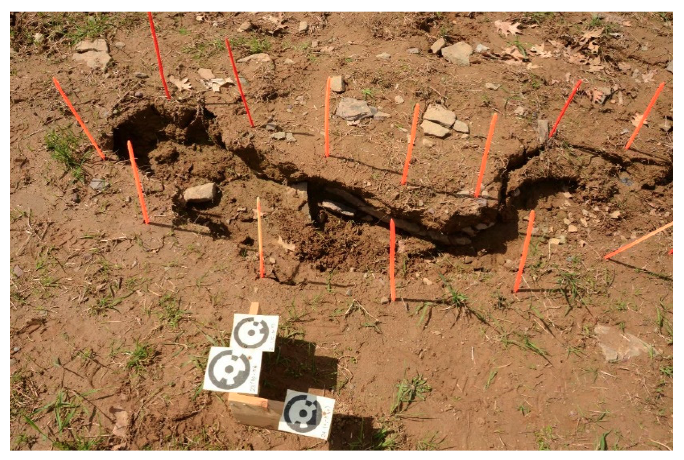
3.2. Soil Surface
3.3. Applicability Analysis
4. Discussion
4.1. Guidance for Using a Consumer-Grade Camera to Measure Water-Induced Channels
4.2. Comparison to Other Methods
4.3. Applications and Future Studies
5. Conclusions
Author Contributions
Funding
Conflicts of Interest
References
- Lal, R. Soil degradation by erosion. Land Degrad. Dev. 2001, 12, 519–539. [Google Scholar] [CrossRef]
- Pimental, D.; Sparks, D.L. Soil as an endangered ecosystem. Bioscience 2000, 50, 947. [Google Scholar] [CrossRef][Green Version]
- Pimentel, D. Soil erosion: A food and environmental threat. Environ. Dev. Sustain. 2006, 8, 119–137. [Google Scholar] [CrossRef]
- Vereecken, H.; Schnepf, A.; Hopmans, J.W.; Javaux, M.; Or, D.; Roose, T.; Vanderborght, J.; Young, M.; Amelung, W.; Aitkenhead, M. Modeling soil processes: Review, key challenges, and new perspectives. Vadose Zone J. 2016, 15. [Google Scholar] [CrossRef]
- Li, S.; Lobb, D.A.; Tiessen, K.H. Soil erosion and conservation based in part on the article “soil erosion and conservation” by w. S. Fyfe, which appeared in the encyclopedia of environmetrics. In Encyclopedia of Environmetrics; El-Shaarawi, A.H., Piegorsch, W.W., Chebana, F., Ouarda, T.B., Eds.; John Wiley & Sons: Hoboken, NJ, USA, 2013; ISBN 0470973889. [Google Scholar]
- Lal, R. Soil Erosion Research Methods, 2nd ed.; St. Lucie Press: Delray Beach, FL, USA, 1994; ISBN 1884015093. [Google Scholar]
- Morgan, R.P.C. Soil Erosion and Conservation, 3rd ed.; Blackwell Pub.: Malden, MA, USA, 2005; ISBN 1405117818. [Google Scholar]
- Hill, W.W.; Kaiser, V.G. Method of Measuring Soil Erosion Losses; Rill and Sheet Erosion; Soil Conservation Service: Washington, DC, USA, 1965; pp. 13–14. [Google Scholar]
- Hudson, N. Field measurements of accelerated soil erosion in localized areas. Rhod. Agric. J. 1964, 31, 46–48. [Google Scholar]
- Casalí, J.; Loizu, J.; Campo, M.; De Santisteban, L.; Álvarez-Mozos, J. Accuracy of methods for field assessment of rill and ephemeral gully erosion. CATENA 2006, 67, 128–138. [Google Scholar] [CrossRef]
- McCool, D.; Dossett, M.; Yecha, S. Portable Rill Meter for Field Measurement of Soil Loss; Erosion and Sediment Transport Measurement: Symposium IAHS Publication: Florence, Italy, 1981; pp. 479–484. [Google Scholar]
- Herweg, K. Field Manual for Assessment of Current Erosion Damage; University of Berne, Switzerland: Berne, Switzerland, 1996; ISBN 3906151077. [Google Scholar]
- Goodwin, N.R.; Armston, J.D.; Muir, J.; Stiller, I. Monitoring gully change: A comparison of airborne and terrestrial laser scanning using a case study from aratula, queensland. Geomo 2017, 282, 195–208. [Google Scholar] [CrossRef]
- Liu, H.; Qian, F.; Ding, W.; Gómez, J.A. Using 3d scanner to study gully evolution and its hydrological analysis in the deep weathering of southern china. CATENA 2019, 183, 104218. [Google Scholar] [CrossRef]
- Wang, Q.; Liu, J.; Wu, L.; Xu, Z.; Fan, S.; Qian, A. Analysis of Gully Erosion Hazard Using High Resolution Terrestrial Lidar. In Proceedings of the 2016 IEEE International Geoscience and Remote Sensing Symposium (IGARSS), Beijing, China, 10–15 July 2016; pp. 7469–7472. [Google Scholar]
- Yermolaev, O.; Gafurov, A.; Usmanov, B. Evaluation of erosion intensity and dynamics using terrestrial laser scanning. Eurasian Soil Sci. 2018, 51, 814–826. [Google Scholar] [CrossRef]
- Obu, J.; Lantuit, H.; Grosse, G.; Günther, F.; Sachs, T.; Helm, V.; Fritz, M. Coastal erosion and mass wasting along the canadian beaufort sea based on annual airborne Lidar elevation data. Geomo 2017, 293, 331–346. [Google Scholar] [CrossRef]
- Ciprian Margarint, M.; Niculita, M.; Tarolli, P. Using UAV and Lidar Data for Gullies Erosion Monitoring; EGU General Assembly: Vienna, Austria, 2019; p. 8461. [Google Scholar]
- Lindsay, J.B.; Francioni, A.; Cockburn, J.M. Lidar DEM smoothing and the preservation of drainage features. Remote Sens. 2019, 11, 1926. [Google Scholar] [CrossRef]
- Fink, C.M.; Drohan, P.J. High resolution hydric soil mapping using Lidar digital terrain modeling. Soil Sci. Soc. Am. J. 2016, 80, 355–363. [Google Scholar] [CrossRef]
- Maune, D.F. Digital Elevation Model Technologies and Applications: The DEM Users Manual, 3rd ed.; Asprs Publications: Bethesda, MA, USA, 2017; ISBN 1570830827. [Google Scholar]
- Matthews, N.A.; U.S. Department of the Interior, Bureau of Land Management. Aerial and Close-Range Photogrammetric Technology: Providing Resource Documentation, Interpretation, and Preservation; U.S. Department of the Interior, Bureau of Land Management, National Operations Center: Denver, CO, USA, 2008.
- Ullman, S. The interpretation of structure from motion. Proc. R. Soc. B 1979, 203, 405–426. [Google Scholar] [CrossRef]
- Lowe, D.G. Distinctive image features from scale-invariant keypoints. Int. J. Comput. Vis. 2004, 60, 91–110. [Google Scholar] [CrossRef]
- Stafford, D.B.; Coastal Engineering Research Center. An Aerial Photographic Technique for Beach Erosion Surveys in North Carolina; U. S. Army Coastal Engineering Research Center: Washington, DC, USA, 1971; p. 115. [Google Scholar]
- Stafford, D.B.; Langfelder, J. Air photo survey of coastal erosion. Photogramm. Eng. 1971, 37, 565–575. [Google Scholar]
- Thomas, A.; Welch, R. Measurement of ephemeral gully erosion. Trans. ASAE 1988, 31, 1723–1728. [Google Scholar] [CrossRef]
- Thomas, A.; Welch, R.; Jordan, T. Quantifying concentrated-flow erosion on cropland with aerial photogrammetry. J. Soil Water Conserv. 1986, 41, 249–252. [Google Scholar]
- Welch, R.; Jordan, T.; Thomas, A. A photogrammetric technique for measuring soil erosion. J. Soil Water Conserv. 1984, 39, 191–194. [Google Scholar]
- Carollo, F.G.; Di Stefano, C.; Ferro, V.; Pampalone, V. Measuring rill erosion at plot scale by a drone-based technology. Hydrol. Processes 2015, 29, 3802–3811. [Google Scholar] [CrossRef]
- Di Stefano, C.; Ferro, V. Measurements of rill and gully erosion in sicily. Hydrol. Processes 2011, 25, 2221–2227. [Google Scholar] [CrossRef]
- D’Oleire-Oltmanns, S.; Marzolff, I.; Peter, K.; Ries, J. Unmanned Aerial Vehicle (UAV) for monitoring soil erosion in morocco. Remote Sens. 2012, 4, 3390–3416. [Google Scholar] [CrossRef]
- Giménez, R.; Marzolff, I.; Campo, M.; Seeger, M.; Ries, J.; Casalí, J.; Alvarez-Mozos, J. Accuracy of high-resolution photogrammetric measurements of gullies with contrasting morphology. Br. Soc. Geomorphol. 2009, 34, 1915–1926. [Google Scholar] [CrossRef]
- Martínez-Casasnovas, J.; Antón-Fernández, C.; Ramos, M. Sediment production in large gullies of the mediterranean area (ne spain) from high-resolution digital elevation models and geographical information systems analysis. Br. Soc. Geomorphol. 2003, 28, 443–456. [Google Scholar] [CrossRef]
- Marzolff, I.; Poesen, J. The potential of 3d gully monitoring with gis using high-resolution aerial photography and a digital photogrammetry system. Geomo 2009, 111, 48–60. [Google Scholar] [CrossRef]
- Marzolff, I.; Poesen, J.; Ries, J.B. Short to medium-term gully development: Human activity and gully erosion variability in selected spanish gully catchments. Landf. Anal. 2011, 17, 111–116. [Google Scholar]
- Smith, M.W.; Vericat, D. From experimental plots to experimental landscapes: Topography, erosion and deposition in sub-humid badlands from structure-from-motion photogrammetry. Earth Surf. Process. Landf. 2015, 40, 1656–1671. [Google Scholar] [CrossRef]
- Wells, R.R.; Momm, H.G.; Castillo, C. Quantifying uncertainty in high-resolution remotely sensed topographic surveys for ephemeral gully channel monitoring. Earth Surf. Dynam. 2017, 5, 347. [Google Scholar] [CrossRef]
- Kropáček, J.; Schillaci, C.; Salvini, R.; Maerker, M. Assessment of gully erosion in the upper awash, central ethiopian highlands based on a comparison of archived aerial photographs and very high resolution satellite images. Geogr. Fis. Din. Quat. 2016, 39, 161–170. [Google Scholar] [CrossRef]
- Balaguer-Puig, M.; Marqués-Mateu, Á.; Lerma, J.L.; Ibáñez-Asensio, S. Estimation of small-scale soil erosion in laboratory experiments with structure from motion photogrammetry. Geomo 2017, 295, 285–296. [Google Scholar] [CrossRef]
- Castillo, C.; Marín-Moreno, V.; Pérez, R.; Muñoz-Salinas, R.; Taguas, E. Accurate automated assessment of gully cross-section geometry using the photogrammetric interface freexsapp. Earth Surf. Process. Landf. 2018, 43, 1726–1736. [Google Scholar] [CrossRef]
- Castillo, C.; Pérez, R.; James, M.R.; Quinton, J.; Taguas, E.V.; Gómez, J.A. Comparing the accuracy of several field methods for measuring gully erosion. Soil Sci. Soc. Am. J. 2012, 76, 1319–1332. [Google Scholar] [CrossRef]
- Eltner, A.; Kaiser, A.; Abellan, A.; Schindewolf, M. Time lapse structure-from-motion photogrammetry for continuous geomorphic monitoring. Earth Surf. Process. Landf. 2017, 42, 2240–2253. [Google Scholar] [CrossRef]
- Gessesse, G.D.; Fuchs, H.; Mansberger, R.; Klik, A.; Rieke-Zapp, D.H. Assessment of erosion, deposition and rill development on irregular soil surfaces using close range digital photogrammetry. Photogramm. Rec. 2010, 25, 299–318. [Google Scholar] [CrossRef]
- Kaiser, A.; Neugirg, F.; Rock, G.; Müller, C.; Haas, F.; Ries, J.; Schmidt, J. Small-scale surface reconstruction and volume calculation of soil erosion in complex moroccan gully morphology using structure from motion. Remote Sens. 2014, 6, 7050–7080. [Google Scholar] [CrossRef]
- Prosdocimi, M.; Burguet, M.; Di Prima, S.; Sofia, G.; Terol, E.; Comino, J.R.; Cerdà, A.; Tarolli, P. Rainfall simulation and structure-from-motion photogrammetry for the analysis of soil water erosion in mediterranean vineyards. Sci. Total Environ. 2017, 574, 204–215. [Google Scholar] [CrossRef] [PubMed]
- Wells, R.R.; Momm, H.G.; Bennett, S.J.; Gesch, K.R.; Dabney, S.M.; Cruse, R.; Wilson, G.V. A measurement method for rill and ephemeral gully erosion assessments. Soil Sci. Soc. Am. J. 2016, 80, 203–214. [Google Scholar] [CrossRef]
- Rieke-Zapp, D.H.; Nearing, M.A. Digital close range photogrammetry for measurement of soil erosion. Photogramm. Rec. 2005, 20, 69–87. [Google Scholar] [CrossRef]
- Butler, J.B.; Lane, S.N.; Chandler, J.H. Assessment of DEM quality for characterizing surface roughness using close range digital photogrammetry. Photogramm. Rec. 1998, 16, 271–291. [Google Scholar] [CrossRef]
- Dai, F.; Feng, Y.; Hough, R. Photogrammetric error sources and impacts on modeling and surveying in construction engineering applications. Vis. Eng. 2014, 2, 2. [Google Scholar] [CrossRef]
- Golparvar-Fard, M.; Bohn, J.; Teizer, J.; Savarese, S.; Peña-Mora, F. Evaluation of image-based modeling and laser scanning accuracy for emerging automated performance monitoring techniques. Automat. Constr. 2011, 20, 1143–1155. [Google Scholar] [CrossRef]
- Mellerowicz, K.T.; Rees, H.W.; Chow, T.L.; Ghanem, I. Soils of the Black Brook Watershed St. Andre parish, Madawaska county, New Brunswick; New Brunswick Dept. of Agriculture and Agriculture Canada: Fredericton, NB, Canada, 1993; p. 42.
- Dall’Asta, E.; Thoeni, K.; Santise, M.; Forlani, G.; Giacomini, A.; Roncella, R. Network design and quality checks in automatic orientation of close-range photogrammetric blocks. Sensors 2015, 15, 7985–8008. [Google Scholar] [CrossRef] [PubMed]
- Klaus, D.T. Surface Triangulation by Linear Interpolation in Intersecting Planes; Proc.SPIE: Paris, France, 1989. [Google Scholar]
- DeRose, R.; Gomez, B.; Marden, M.; Trustrum, N. Gully erosion in Mangatu Forest, New Zealand, estimated from digital elevation models. Earth Surf. Process. Landf. 1998, 23, 1045–1053. [Google Scholar] [CrossRef]
- Glendell, M.; McShane, G.; Farrow, L.; James, M.R.; Quinton, J.; Anderson, K.; Evans, M.; Benaud, P.; Rawlins, B.; Morgan, D. Testing the utility of structure-from-motion photogrammetry reconstructions using small Unmanned Aerial Vehicles and ground photography to estimate the extent of upland soil erosion. Earth Surf. Process. Landf. 2017, 42, 1860–1871. [Google Scholar] [CrossRef]
- James, L.A.; Watson, D.G.; Hansen, W.F. Using Lidar data to map gullies and headwater streams under forest canopy: South carolina, USA. CATENA 2007, 71, 132–144. [Google Scholar] [CrossRef]
- Robichaud, P.R.; Wagenbrenner, J.W.; Brown, R.E. Rill erosion in natural and disturbed forests: 1. Measurements. Water Resour. Res. 2010, 46. [Google Scholar] [CrossRef]


| Acronym | VU | AU | HU | DU | WU | VV | AV | HV |
|---|---|---|---|---|---|---|---|---|
| Shape | U-shape | U-shape | U-shape | U-shape | U-shape | V-shape | V-shape | V-shape |
| Orientation | Vertical | Angled | Horizontal | Vertical | Vertical | Vertical | Angled | Horizontal |
| Size | Regular | Regular | Regular | Deep | Wide | N/A | N/A | N/A |
| Tech Specs | |
|---|---|
| Effective Pixels (Megapixels) | 16.2 million |
| Image Sensor Size (mm) | 23.6 × 15.6 |
| Image Sensor Format | DX |
| Image Sensor Type | CMOS |
| Total Pixels (Megapixels) | 16.9 million |
| Image Pixel Size (μm) | 4.78 |
| Image Area (pixels) | 4928 × 3262 |
| Approx. Weight (g) | 690 |
| Channel | Shooting Angle (with 80% Overlap) | Image Overlap Rate (with 70° Angle) | ||||||||||
|---|---|---|---|---|---|---|---|---|---|---|---|---|
| 90° | 80° | 70° | 60° | 45° | 30° | 90% | 80% | 70% | 60% | 50% | ||
| VU | Average | 29.0 | 30.0 | 31.0 | 28.6 | 27.0 | 21.3 | 27.4 | 31.0 | 26.9 | 25.8 | 20.4 |
| SD | 3.8 | 1.2 | 3.4 | 3.7 | 3.6 | 5.6 | 2.9 | 3.4 | 3.8 | 3.3 | 13.6 | |
| ME | −10.0 | −9.0 | −8.0 | −10.4 | −12.0 | −17.7 | −5.5 | −8.0 | −12.1 | −13.1 | −18.6 | |
| RMSE | 10.6 | 9.0 | 8.6 | 10.9 | 12.5 | 18.5 | 6.1 | 8.6 | 12.6 | 13.5 | 22.4 | |
| AU | Average | 26.7 | 27.3 | 28.6 | 30.6 | 27.9 | 19.6 | 24.6 | 28.6 | 29.0 | 27.2 | 13.8 |
| SD | 4.9 | 3.5 | 2.9 | 3.1 | 13.0 | 9.2 | 3.5 | 2.9 | 2.0 | 4.7 | 7.1 | |
| ME | −14.4 | −13.8 | −12.4 | −10.6 | −13.2 | 21.4 | −9.7 | −12.4 | −12.0 | −14.0 | −27.4 | |
| RMSE | 15.1 | 14.3 | 12.7 | 11.0 | 18.0 | 23.2 | 10.3 | 12.7 | 12.2 | 14.7 | 28.3 | |
| HU | Average | 28.4 | 25.5 | 33.1 | 34.6 | 22.4 | 18.0 | 27.3 | 33.1 | 34.0 | 24.6 | 18.7 |
| SD | 5.1 | 3.4 | 3.0 | 7..8 | 7.6 | 9.9 | 3.3 | 3.0 | 2.9 | 7.4 | 11.8 | |
| ME | −10.4 | −13.4 | −5.7 | −4.2 | −16.4 | −20.8 | −3.4 | −5.7 | −4.8 | −14.2 | −20.1 | |
| RMSE | 11.6 | 13.8 | 6.3 | 8.4 | 17.8 | 22.7 | 4.7 | 6.3 | 5.5 | 16.0 | 23.1 | |
| DU | Average | 60.6 | 56.5 | 52.1 | 63.4 | 55.0 | 44.5 | 64.5 | 52.1 | 48.8 | 50.6 | 72.3 |
| SD | 4.9 | 4.5 | 4.0 | 8.5 | 6.3 | 12.0 | 3.1 | 4.0 | 2.9 | 4.4 | 27.4 | |
| ME | −17.8 | −21.8 | −26.3 | −14.9 | −23.4 | −33.7 | −22.3 | −26.3 | −29.6 | −27.8 | −6.5 | |
| RMSE | 18.2 | 22.1 | 26.5 | 17.0 | 24.1 | 35.5 | 22.6 | 26.5 | 29.7 | 28.2 | 27.0 | |
| WU | Average | 64.8 | 59.9 | 62.8 | 67.0 | 72.2 | 65.6 | 64.7 | 62.8 | 66.7 | 63.6 | 49.7 |
| SD | 3.0 | 2.5 | 3.0 | 9.4 | 6.8 | 16.7 | 2.8 | 3.0 | 5.0 | 3.7 | 11.9 | |
| ME | −9.6 | −18.1 | −15.2 | −11.0 | −5.6 | −12.4 | −8.4 | −15.2 | −11.2 | −14.4 | −28.3 | |
| RMSE | 13.5 | 18.4 | 15.6 | 14.0 | 8.8 | 19.9 | 9.0 | 15.6 | 12.4 | 14.7 | 30.6 | |
| Channel | Shooting Angle (with 80% Overlap) | Image Overlap Rate (with 70° Angle) | ||||||||||
|---|---|---|---|---|---|---|---|---|---|---|---|---|
| 90° | 80° | 70° | 60° | 45° | 30° | 90% | 80% | 70% | 60% | 50% | ||
| VV | ME | 1.5 | −0.8 | −0.6 | 6.2 | 5.1 | 4.8 | 2.3 | −0.6 | 0.2 | 0.1 | −1.5 |
| RMSE | 2.7 | 3.0 | 1.3 | 10.4 | 8.3 | 8.6 | 4.0 | 1.3 | 1.9 | 2.4 | 2.4 | |
| AV | ME | 3.8 | −0.4 | −0.4 | 9.2 | 3.8 | −12.9 | 4.5 | −0.4 | 3.6 | −8.4 | −3.7 |
| RMSE | 4.9 | 5.1 | 1.6 | 12.7 | 9.1 | 18.3 | 5.6 | 1.6 | 5.7 | 7.9 | 21.8 | |
| HV | ME | −2.5 | −5.5 | −6.2 | 9.2 | 6.0 | −1.6 | 7.5 | −6.2 | −5.5 | N/A | N/A |
| RMSE | 9.3 | 8.9 | 8.9 | 11.9 | 8.4 | 19.0 | 9.7 | 8.9 | 7.0 | N/A | N/A | |
| Transect | 1 | 2 | 3 | 4 | 5 | 6 | 7 | 8 | 9 | 10 | Average | RMSE (cm2) |
|---|---|---|---|---|---|---|---|---|---|---|---|---|
| Manual measurement | 482.0 | 506.2 | 498.8 | 480.1 | 376.2 | 487.1 | 489.7 | 853.1 | 749.1 | 537.4 | ||
| ME (cm2) | 6.8 | 4.2 | −7.5 | −3.9 | 11.7 | 0.2 | −7.8 | 17.7 | −7.3 | 6.0 | 2.0 | 8.6 |
| ME (%) | 1.4 | 0.8 | −1.5 | −0.8 | 3.1 | 0.0 | −1.6 | 2.1 | −1.0 | 1.1 | 0.3 |
| Shooting Angle (°) | Image Overlapping Rate (%) | Data Collection Time (min) | Detection Area Limit (m2) |
|---|---|---|---|
| 90 | 80 | 13 | 3.6 |
| 80 | 80 | 13 | 4.1 |
| 70 | 80 | 13 | 5.5 |
| 60 | 80 | 13 | 6.2 |
| 45 | 80 | 13 | 10.8 |
| 30 | 80 | 13 | 18 |
| 70 | 90 | 15 | 5.5 |
| 70 | 80 | 13 | 5.5 |
| 70 | 70 | 10 | 5.5 |
| 70 | 60 | 9 | 5.5 |
| 70 | 50 | 8 | 5.5 |
© 2020 by the authors. Licensee MDPI, Basel, Switzerland. This article is an open access article distributed under the terms and conditions of the Creative Commons Attribution (CC BY) license (http://creativecommons.org/licenses/by/4.0/).
Share and Cite
Zheng, F.; Wackrow, R.; Meng, F.-R.; Lobb, D.; Li, S. Assessing the Accuracy and Feasibility of Using Close-Range Photogrammetry to Measure Channelized Erosion with a Consumer-Grade Camera. Remote Sens. 2020, 12, 1706. https://doi.org/10.3390/rs12111706
Zheng F, Wackrow R, Meng F-R, Lobb D, Li S. Assessing the Accuracy and Feasibility of Using Close-Range Photogrammetry to Measure Channelized Erosion with a Consumer-Grade Camera. Remote Sensing. 2020; 12(11):1706. https://doi.org/10.3390/rs12111706
Chicago/Turabian StyleZheng, Fangzhou, Rene Wackrow, Fan-Rui Meng, David Lobb, and Sheng Li. 2020. "Assessing the Accuracy and Feasibility of Using Close-Range Photogrammetry to Measure Channelized Erosion with a Consumer-Grade Camera" Remote Sensing 12, no. 11: 1706. https://doi.org/10.3390/rs12111706
APA StyleZheng, F., Wackrow, R., Meng, F.-R., Lobb, D., & Li, S. (2020). Assessing the Accuracy and Feasibility of Using Close-Range Photogrammetry to Measure Channelized Erosion with a Consumer-Grade Camera. Remote Sensing, 12(11), 1706. https://doi.org/10.3390/rs12111706