RL-AKF: An Adaptive Kalman Filter Navigation Algorithm Based on Reinforcement Learning for Ground Vehicles

Abstract

Kalman filter is a commonly used method in the Global Navigation Satellite System (GNSS)/Inertial Navigation System (INS) integrated navigation system, in which the process noise covariance matrix has a significant influence on the positioning accuracy and sometimes even causes the filter to diverge when using the process noise covariance matrix with large errors. Though many studies have been done on process noise covariance estimation, the ability of the existing methods to adapt to dynamic and complex environments is still weak. To obtain accurate and robust localization results under various complex and dynamic environments, we propose an adaptive Kalman filter navigation algorithm (which is simply called RL-AKF), which can adaptively estimate the process noise covariance matrix using a reinforcement learning approach. By taking the integrated navigation system as the environment, and the opposite of the current positioning error as the reward, the adaptive Kalman filter navigation algorithm uses the deep deterministic policy gradient to obtain the most optimal process noise covariance matrix estimation from the continuous action space. Extensive experimental results show that our proposed algorithm can accurately estimate the process noise covariance matrix, which is robust under different data collection times, different GNSS outage time periods, and using different integration navigation fusion schemes. The RL-AKF achieves an average positioning error of 0.6517 m within 10 s GNSS outage for GNSS/INS integrated navigation system and 14.9426 m and 15.3380 m within 300 s GNSS outage for the GNSS/INS/Odometer (ODO) and the GNSS/INS/Non-Holonomic Constraint (NHC) integrated navigation systems, respectively.

1. Introduction

Precise positioning and navigation of ground vehicles in complex urban environments is fundamental and necessary for the development of efficient stroke planning, unmanned driving, and autonomous operation. With the worldwide deployment of the Global Navigation Satellite System (GNSS) and the Inertial Navigation System (INS), many research efforts have been made to estimate the dynamic states of ground vehicles and improve the estimation accuracy using GNSS and INS data [1,2,3,4,5], among which the Kalman filtering (KF) techniques play an essential role [6].

The KF is an optimal state estimator for linear Gaussian state-space models and is the most common technique for carrying out the GNSS/INS integrated navigation task [7]. KF series algorithms can provide optimal solutions if the system process noise models are correctly defined, and the process noise statistics are completely known [1,8]. The conventional method of determining the covariance matrices of process noise (Q) for KF mostly relies on the calibrated results provided by the manufacturer using the Allan variance algorithm [9] from each type of sensor and then fixing them. The process noise represents the feature that the state of the system changes in accordance with time, the environment, and the sensor device itself. However, it is difficult to know the exact details of when and how these changes occur [10]. Assume that the Q are perturbed, how would such perturbations affect the optimality of the filter? One stability consideration was presented in [8,11], where it is shown that incorrect values of the process noise covariance matrix can cause the filter to diverge; i.e., the variance of a linear combination of the estimation error becomes unbounded [12,13]. We experimentally verified the influence of different process noise covariance matrices on the integrated navigation positioning performance. Taking the calibration results of sensor manufacturers as the standard value, the variation of positioning error with matrix Q is plotted in Figure 1, which confirms that matrix Q has an obvious influence on positioning accuracy.

Several results which deal with the deviation from the basic assumptions that guarantee optimality, for example, zero-mean and constant-variance Gaussian models of the errors, are presented in the literature, such as in [14,15,16,17], where the robustness of the filter is considered. There are some online identification schemes which identify Q from the innovation sequence, but their assumptions are rather restrictive and are not applicable for general system [18]. The results of [12] constrain the uncertainties to a scalar multiple of the ideal model; e.g., for the process noise covariance matrix, we have $Q^{\prime }=\alpha Q$, where $\alpha$ is the learned zoom factor. This constraint appears to be quite restrictive.

Accurate and continuous positioning of ground vehicles is a main requirement of autonomous vehicle mapping systems [19]. GNSS is a key technology to meet this demand in outdoor environments [20]. However, in densely built-up areas such as urban canyons and through tunnels, GNSS observations, which may suffer from outages, jamming, and multipath effects, are not properly available [21]. Inertial Navigation Systems (INS), on the other hand, are autonomous systems that are immune to external interference, but their accuracy deteriorates in the long term due to the sensor’s bias error drift, scale factor instability, and misalignment [22,23]. Integrating both INS and GNSS with KF can provide superior performance than any of them operating alone. There are many different types of sensors that can be used to navigate ground vehicles and are highly adaptable to complex urban environments, such as Lidar [24], lane-boundary [25,26,27], map matching [26,28], and stereo visual [19,29,30,31,32]. However, comprehensively considering the equipment cost and positioning accuracy, the GNSS/INS integrated navigation system is currently still the most widely used. In the integrated navigation system, the KF as an effective optimal state estimation method has been widely used [33]. However, the KF performs unsatisfactorily when applied to nonlinear system problems [34]. An approach coupled with the extended Kalman filter (EKF) [35] algorithm and interactive multi-model has therefore been proposed to deal with unrealistic noise considerations and allows the use of highly dynamic models in no maneuvering situations. Because the EKF is sensitive to linearization errors, an unscented Kalman filter (UKF) [36,37,38,39] with different noise covariances integrated with the interactive multi-model has been introduced into the framework of integration to compensate for filter divergence. However, there is a limitation of the KF algorithm due to the necessity of having a prior statistical value of process and measurement noise. If the mathematical model of the integrated navigation system (including the system dynamics model and statistical properties of process noise and measurement noise, etc.) is precisely known, the KF algorithms can be used to get the real-time accurate state estimation [7,8,40].

However, the constructions of accurate mathematical models are very difficult and need a lot of experimentation, especially concerning the accurate statistical properties of process noise covariance matrices. To solve this problem, many studies have been carried out which constantly estimate or correct the process noise covariance matrix online or offline [1,6,7,8,10,12,41]. The existing process noise covariance estimation algorithms of KF can be roughly categorized as innovation-based estimation, covariance scaling, and feedback correction. When the variance of Kalman gain is assumed to be negligible for stable Kalman estimation, Wang et al. [1] and Akhlaghi et al. [6] calculated the process noise covariance from the innovation sequence for the adaptive estimation of Q. Ngoc et al. [10] modeled the process noise covariance as a function of the speed noise power spectral densities, the clock bias noise, and frequency drift noise. However, concerning the dynamic case, this innovation-based estimation algorithm is not accurate or even inapplicable. To improve the robustness of the adaptive filtering algorithm for the process noise covariance matrix estimation, Ding et al. [41] proposed a scaling method. It assumes that the Q matrix between adjacent moments has a proportional relationship. Moreover, the scaling factor implies a rough ratio between the calculated process noise covariance and the predicted one. On the basis of this work, Rui et al. [42] propose a method to automatically identify and eliminate the instantaneous interference based on K-means clustering, which guarantees that only stable measurement errors can be used to calibrate noise estimation. This method is more robust due to fewer parameters, but it can only zoom in and out on the magnitude of the process noise covariance matrix rather than individual elements. Riboni et al. [43] take both Q and R into consideration and establish a back propagation model of the positioning error to study both of them. Not exactly using the chain rule to calculate the gradient, this paper uses the Nelder–Mead algorithm to approximate it.

To overcome the problems of difficult gradient feedback and model limitation in the above literature, we use reinforcement learning, which has a strong automatic exploitation ability, to adaptively search for the optimal process noise covariance matrix in the continuous space through the reward maximization mechanism. In [44], RL was applied to Gaussian processes for mobile robots. A similar method is used in [45], where they are used to find parameters of a controller for a small blimp. However, these methods do not find the Q parameters of KF, which play an important role in determining the system stability [46]. The deep-Q-network (DQN) based method was developed to solve these problems [47]. However, the DQN-based [48] method has the following problems: (1) The action space is limited because the DQN is only applicable to the discrete action space; (2) the size of the neural network becomes larger as the discretization step becomes smaller, which requires much training time and memory. To alleviate the problem of the DQN-based method, the deep deterministic policy gradient (DDPG) [49] algorithm, which is a variant of the actor–critic algorithm for deep reinforcement learning, is used. The DDPG algorithm has been successfully applied to high-dimensional and end-to-end reinforcement learning problems such as simulation games and virtual physical environments.

In summary, the process noise covariance matrix has a great influence on the positioning performance of KF but the previous studies have not yet provided a comprehensive estimation method which can give a definite process noise covariance matrix and maintain accuracy and robustness. In this study, we demonstrate an adaptive Kalman filter navigation algorithm (RL-AKF) to adjust the process noise covariance matrix elastically using the DDPG method. By taking the integrated navigation system as the environment and the opposite of the current positioning error as the reward, the adaptive Kalman filter navigation algorithm uses the deep deterministic policy gradient to obtain the most optimal process noise covariance matrix estimation from the continuous action space. Extensive experiments are performed to demonstrate that the developed method successfully finds the Q parameters so as to obtain the most optimal navigation accuracy.

To solve the above-mentioned problems, we propose an adaptive process noise covariance estimation algorithm driven by the positioning accuracy using reinforcement learning (RL). RL [50] is a class of machine learning methods for solving sequential decision-making problems that can be described as Markov decision processes (MDPs) [51] by the trial and error method using the environment information, which has a strong automatic exploitation ability [52]. By taking the integrated navigation system as the environment and the negative of the positioning error as the reward, our proposed adaptive Kalman filter navigation algorithm uses the deep deterministic policy gradient to obtain the most optimal state estimation, i.e., the process noise covariance matrix in the continuous action space.

The main contributions of this paper are summarized as follows:

• We propose a novel adaptive Kalman filter navigation algorithm RL-AKF based on reinforcement learning. This algorithm can achieve accurate and robust navigation performance by automatically learning an optimal process noise covariance matrix online from low-cost MEMS IMU and GNSS data over a short period of time without affecting the normal navigation process.
• We design the reward of reinforcement learning as the negative of the location error. This scheme solves the difficulty of the gradient calculation and enables the current process noise covariance matrix to be updated effectively toward the direction of reducing the position error.
• We design the state and action space for adaptive process noise covariance matrix estimation. We introduce the Deep Deterministic Policy Gradient (DDPG) method to obtain an optimal state estimation from continuous action space. We also propose an exponential strategy to meet the semi-positive definite requirement of the covariance matrix.
• We evaluate our proposed algorithm with extensive practical data. The experimental results demonstrate that our proposed RL-AKF algorithm can obtain excellent performances, including position, velocity, and course angle, under different data collection times, various GNSS outage periods, and different integration navigation schemes.

The rest of this paper is organized as follows. Within discussing the related work, we provide several existing algorithms of adaptive navigation. We then show how we establish the RL network for adaptive estimation of the process noise covariance matrix in the Kalman filter from the raw sensor data in Section 3, followed by an experimental evaluation and comparison with other state-of-art algorithms. We conclude our work in Section 5.

Table 1. Description of Notation.

Field	Symbol	Description
Kalman filter	$\delta x$	Error state in the prediction phase
	$P$	The covariance matrix of the predicted error
	$\delta z$	Error state obtained from the measurement
	H	The observation matrix
	$Q$	Process noise covariance matrix
	$R$	Measurement noise covariance matrix
RL	$s$	State of RL, which is defined as the value of the current process noise
	$\alpha$	Action of RL, which is defined as the change of the current process noise
	$r$	Reward of RL
	$E$	Environment of RL
DDPG	${\theta }^{\mu }$,${\theta }^{\mu \prime }$	The parameters of Actor network
	${\theta }^{\nu }$,${\theta }^{\nu \prime }$	The parameters of Critic network
Sensors	${\omega }_t^{IMU},{\alpha }_t^{IMU}$	Gyroscope and acceleration output at time t
	$r_t^{IMU}$	The predicted position at time t
	$r_t^{RTK}$	The measurement position at time t

lists the main mathematical notations used in this paper.

2. Materials and Methods

2.1. System Overview

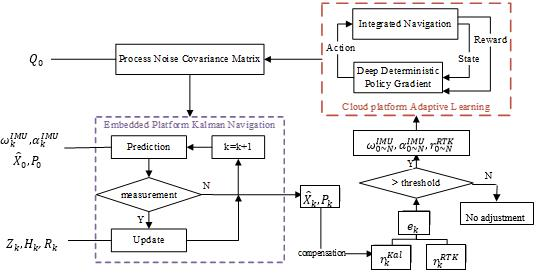
Our proposed adaptive Kalman filter navigation algorithm RL-AKF is mainly composed of integrated navigation based on the Kalman filter and adaptive process noise covariance matrix estimation using reinforcement learning. The system overview is shown in Figure 2.

The idea of the RL-AKF algorithm is to realize the high-accuracy positioning of the integrated navigation system by adaptively adjusting the Q matrix. The algorithm obtains the input ${\omega }_k^{IMU}$ of the gyroscope and the input ${\alpha }_k^{IMU}$ of the acceleration at each IMU data update time. Given the initial state ${\widehat{X}}_0$ and initial state covariance matrix $P_0$, the embedded platform Kalman navigation module calculates the prediction error state $X_k$ once the IMU data is updated. If the GNSS measurement inputs $Z_k, H_k$ and $R_k$ exist at the current moment, the module will carry out a measurement update to obtain the final error state estimation result ${\widehat{X}}_k$. Then the current position estimation result $r_k^{Kal}$ is obtained after the error compensation.

At the beginning of the algorithm’s operation, the Q matrix in this process is provided by the default value $Q_0$ (calibration result of the product or the estimation result of the previous RL-AKF). Considering that the GNSS carrier phase differential positioning results (RTK) have the characteristics of high accuracy but high environmental requirements, the RL-AKF algorithm will consistently monitor the GNSS positioning status. Once it is detected that the current positioning result is RTK differential positioning, the algorithm will calculate the positioning error of the current KF system. If the calculated error is greater than the threshold, it means that there is a certain deviation in the Q matrix, which leads to inaccurate KF results. Then the RL-AKF algorithm collects N seconds of IMU and GNSS data nearest to the current moment, performs adaptive learning of the process noise covariance matrix, and finally feedbacks the learned Q matrix to the previous KF system to continue filtering and positioning.

The target of the cloud platform adaptive learning module is to learn a process noise covariance matrix which is able to minimize the location error of the collected data using the RL algorithm. The elements of RL are defined as follows.

State$\mathrm{s}$: The current value of process noise vector W. The estimation target Q matrix is the covariance of the W vector.

Action$\mathsf{\alpha }$: The change of noise vector W. The $\mathsf{\alpha }$’s dimension is six because six noise values make up the W vector. Obviously, the action is defined in the continuous real number space.

Reward$r:$ The opposite of the location error. The bigger the reward, the better the current navigation result.

Environment: The GNSS/INS integration navigation model. Once the environment receives a new action, it updates the current state and calculates the location error to get a reward. Then it passes the reward to the agent.

Agent: The decision model of RL. We use the Deep Deterministic Policy Gradient (DDPG) algorithm, which adopts a network to fit the strategy function in the aspect of action output, to deal with the challenge of continuous action space.

The implemented tasks conform to the standard interface of an infinite-horizon discounted Markov decision process (MDP), defined by the tuple ($\mathrm{s},\mathsf{\alpha },\mathrm{P},\mathrm{r},{\rho }_0$), where $\mathrm{s}$ is an infinite set of states, $\mathsf{\alpha }$ is a set of actions, $\mathrm{P}:\mathrm{s}\times \mathsf{\alpha }\times \mathrm{s}\to {\mathbb{R}}_{\ge 0}$ is the transition probability distribution represented by the agent, $\mathrm{r}:\mathrm{s}\times \mathsf{\alpha }\to \mathbb{R}$ is the reward value obtained from the environment, and ${\rho }_0:\mathrm{s}\to {\mathbb{R}}_{\ge 0}$ is the initial state. These characteristics allow the RL-AKF to be formalized as an MDP where operator actions cause state transitions, which affect the ramp-up value of reward. Capturing the dependencies between actions and reactions allows the machine learning methods to be used to find good policies for the ramp-up of observed states, from which we can also obtain the learned optimal state.

2.2. Environment Definition

Inertial navigation is a kind of projection and integral operation. Its navigation error accumulates with time. Therefore, INS needs to be combined with other navigation and positioning methods to solve the problem of accuracy divergence. Integrated navigation is a technique that uses the complementary information provided by multiple sensors to improve the accuracy and redundancy of the navigation system. The effective fusion of data from multiple sensors requires the selection of an appropriate optimal estimation algorithm.

The value of the process noise covariance matrix has a direct impact on the positioning accuracy of the integrated navigation system. In this paper, we locate the environment factor of reinforcement learning as the integrated navigation system based on the Kalman filter. This environment will give an evaluation of the pros and cons of the current covariance matrix. The overall calculation process can be divided into forwarding INS mechanization, error model update, and feedback correction.

2.2.1. Forwarding INS Mechanization

To initialize the INS system, the alignments of the position ($r_0$), the velocity ($v_0$) and the attitude (${\psi }_0$) have to be done. The first two can be obtained directly from the GNSS measurement, and the attitude alignment can be achieved by stationary alignment [22] or in-motion alignment [53] methods.

Shin et al. [37] have covered the forward INS mechanization algorithm in detail. It takes the attitude ${\psi }_{k-1}$, velocity $v_{k-1}$, and position $r_{k-1}$ at time $t_{k-1}$, gyrometer incremental angles $\mathsf{\Delta }{\tilde{\theta }}_k$, and acceleration incremental velocities due to the specific force $\mathsf{\Delta }{\tilde{v}}_k$ from $t_{k-1}$ to $t_k$ as the input to calculate the attitude ${\widehat{\psi }}_k^{IMU}$, velocity ${\widehat{v}}_k^{IMU}$, and postion ${\widehat{r}}_k^{IMU}$ at time $t_k$.

2.2.2. Error Model Based on Kalman Filter

In our navigation system, an error model is used to describe the relationship between the prediction, i.e., ${\widehat{r}}_k^{IMU}$, and the measurement, i.e., $r_k^{RTK}$. The error state vector of the prediction stage is defined as

$$\delta x={\left[\begin{array}{ccc}\delta r^T& \delta v^T& \begin{array}{ccc}{\varphi }^T& b_g^T& \begin{array}{ccc}{b}_a^T& s_g^T& s_a^T\end{array}\end{array}\end{array}\right]}^T$$

(1)

where $\delta r$, $\delta v$, and $\varphi$ represent the error of position, velocity, and attitude, which can be written as follows:

$$\delta r=\left[\begin{array}{ccc}\delta r_N& \delta r_E& \delta r_D\end{array}\right]$$

(2)

$$\delta v=\left[\begin{array}{ccc}\delta v_N& \delta v_E& \delta v_D\end{array}\right]$$

(3)

$$\varphi =\left[\begin{array}{ccc}{\varphi }_{roll}& {\varphi }_{pitch}& {\varphi }_{course}\end{array}\right]$$

(4)

where $b_g$ denotes the gyro biases; $b_a$, the accelerometer biases; $s_g$, the gyro scale; and $s_a$, the accelerometer scale. These errors are all represented by a three-dimensional vector. In the prediction stage, the estimate and its error covariance are projected ahead as follows:

$$\delta {\widehat{x}}_{k|k-1}={\mathsf{\Phi }}_{k-1}\delta {\widehat{x}}_{k-1|k-1}+{\mathsf{\Gamma }}_{k|k-1}{W}_{k-1}$$

(5)

$$P_{k|k-1}={\mathsf{\Phi }}_{k-1}{P}_{k-1|k-1}{\mathsf{\Phi }}_{k-1}^T+Q_{k-1}$$

(6)

where $\delta {\widehat{x}}_{k-1|k-1}$ and $P_{k-1|k-1}$ are the integrated navigation result at time k-1, while $\delta {\widehat{x}}_{k|k-1}$ and $P_{k|k-1}$ represent the INS prediction result at time k from the navigation result at time k-1. ${\mathsf{\Phi }}_{k-1}$ is the state transition matrix, ${\Gamma }_{k|k-1}$ is the process noise distribution matrix, and $W_{k-1}$ is the process noise vector, where $E\left[W_k{W}_k^T\right]=Q_k$.

Once receiving a new measurement $r_k^{RTK}$, the error measurement $\mathsf{\delta }{z}_k$ will be calculated first as Equation (7) shows:

$$\delta z_k={\widehat{r}}_k^{IMU}-r_k^{RTK}$$

(7)

After the Kalman gain $K_k$ is computed, the error state vector and the error covariance are updated using the predicted estimate, $\mathsf{\delta }{\widehat{x}}_{k|k-1}$, and its covariance matrix, $P_{k|k-1}$:

$$K_k=P_{k|k-1}{H}_k^T{\left(H_k{P}_{k|k-1}{H}_k^T+R_k\right)}^{-1}$$

(8)

$$\mathsf{\delta }{\widehat{x}}_{k|k}=\mathsf{\delta }{\widehat{x}}_{k|k-1}+K_k\left(\delta z_k-H_k\mathsf{\delta }{\widehat{x}}_{k|k-1}\right)$$

(9)

$$P_{k|k}=\left(I-K_k{H}_k\right)P_{k|k-1}{\left(I-K_k{H}_k\right)}^T+K_k{R}_k{K}_k^T$$

(10)

where $R_k$ is the measurement noise covariance matrix and $H_k$ is a matrix used to unify the units and scales between the prediction and the measurement.

2.2.3. Feedback Correction

The $\delta r_{k|k}$ in the error state vector explicitly represents the difference between the mechanization result and the final navigation position. In low latitudes, the navigation position can be obtained directly through the error compensation as:

$$r_k^{IMU}={\widehat{r}}_k^{IMU}+\delta r_k$$

(11)

2.3. State Definition

2.3.1. Components of the Q Matrix

The sensor manufacturer usually provides a set of default calibration values for the corresponding type of the sensor. In this section we provide the components and the initial value of the process noise covariance matrix, which is shown in Equation (12).

$$W_k={[w_{\delta r},w_{\delta v},w_{\phi },w_q,w_{\nabla },w_{\delta kii}]}^T$$

(12)

$$Q=E[W_k{W}_k^T]$$

(13)

where $W_k$ is the process noise vector with $21\mathrm{x}1$ dimension, and Q is the covariance of this vector. The meaning of each component of the noise vector and its initial value are shown in

Table 2. Initial Values of Matrix Q.

Symbol	Meaning	Dim	M39	CPT
$w_{\delta r}$	position walk coefficient	3	0$m/\sqrt{h}$	0$m/\sqrt{h}$
$w_{\delta v}$	velocity random walk	3	0.09$m/s/\sqrt{h}$	~$m/s/\sqrt{h}$
$w_{\varphi }$	angle random walk	3	0.12$deg/\sqrt{h}$	0.067$deg/\sqrt{h}$
$w_q$	angular rate random walk	3	180$deg/\sqrt[2]{h^3}$	~$deg/\sqrt[2]{h^3}$
$w_{\nabla }$	acceleration random walk	3	8$\mu Gal/\sqrt{h}$	~$\mu Gal/\sqrt{h}$
$w_{\delta kii}$	scale error random walk	6	1000$ppm/\sqrt{h}$	4000$ppm/\sqrt{h}$

, which is based on the manufacturer’s calibration results.

2.3.2. Construction of Positive Semi-Definiteness for Matrix Q

The prerequisite of calculating matrix Q using Equation (13) is that all the estimated states of reinforcement learning are positive semi-definite matrices. The current state transition method cannot guarantee this requirement. We refactor the calculation method of Q so that the new state always satisfies this condition.

Since Q is a diagonal matrix, the Q matrix is a positive semi-definite matrix as long as the diagonal elements are constrained to non-negative. We propose a simple way to enforce this constraint by adding an element-wise exponential function to the diagonal vector, i.e., updating the Q matrix according to Equation (14).

$$Q=E[e^{W_k}{(e^{W_k})}^T]$$

(14)

The state change is defined on the current $W_k$. When a new action $a_k$ is executed, the new state Q’ will be expressed as:

$$Q\prime =E[e^{W_k+a_k}{(e^{W_k+a_k})}^T]$$

(15)

2.4. Reward Definition

When the environment receives an action that causes a state change, we need to define a sufficient reward mechanism to evaluate the current action. For this problem, we modeled the reward as the opposite of the location error over the N seconds of IMU and GNSS data.

We select $\mathrm{m}$ segments with the length of $l_m$ from the N seconds of data. To simulate the outage of GNSS signals, we will not carry out the GNSS measurement update during these segments in the Kalman filter navigation process. We calculate the positioning error at the end of each segment and then obtain the root mean square error over m errors as the final navigation accuracy under the current process noise covariance matrix. The reward value is configured to the opposite of the final localization error. By maximizing the reward, we will finally obtain the process noise covariance matrix, which can minimize the positioning error.

2.5. Agent Definition

For the adaptive process noise covariance matrix estimation problem, the action space is defined in the real number field, $\left[{\mathcal{L}}_p,{\mho }_p\right]$. We need an algorithm that can choose optimal action from the continuous space instead of a simple Q(s, a) table.

2.5.1. Action Generation with DDPG

DDPG is an actor–critic, model-free algorithm based on the deterministic policy gradient that can operate over continuous action spaces and it includes two neural networks (NNs), a critic NN introduced to evaluate the long-time performance of the designed control in the current time step and an action NN used to output continuous action in the corresponding state [49]. Moreover, in order to improve learning efficiency and prevent local optimality, an experience replay memory is created to store historical samples, each time a certain number of samples are randomly selected for training. The application framework of DDPG in adaptive process noise covariance matrix estimation of integrated navigation is shown in Figure 3.

In each episode, the DDPG executes a certain time step. At each time step, the action $a_i$ is selected by the action evaluation network of the ACTOR module, which is based on the cost function that maximizes the reward from taking accurate action. Then Uhlenbeck–Ornstein stochastic process (UO process) is added to the learned action as a random noise since it has a good correlation in time, which can make the agent explore the environment much better. The GNSS/INS integration navigation model executes this action, calculates the reward, and stores the transition data in the experience replay memory. When the size of the memory meets the requirements, the DDPG will randomly sample batch-sized training samples to calculate the gradient of the value evaluation net and action evaluation network, separately. Then, it updates the network weight for the next round of calculation. The algorithm process is described in Algorithm 1.

Algorithm 1. Adaptive process noise covariance matrix estimation based on DDPG.

Input: Continuous-time series IMU sensor data and GNSS data Output: Final state as the optimal process noise covariance matrix.

Construct an action evaluation network and a value evaluation network. The input size of the action net is $\mathrm{s}\_\dim$=21, and the output size is $\mathrm{a}\_\dim$=6. As for value net, the former is $\mathrm{s}\_\dim +\mathrm{a}\_\dim$=27 and the latter represents $\mathsf{\upsilon }\left(\mathrm{s},\mathrm{a}\right)$ with dimension 1 Initialize the weights of the two networks as ${\theta }^{\mu }$ and ${\theta }^{\upsilon }$. Copy the network and parameters as the action target network and the value target network: ${\theta }^{\mu }\to {\theta }^{{\mu }^{\prime }},{\theta }^{\upsilon }\to {\theta }^{{\upsilon }^{\prime }}$ Initialize experience replay memory with capacity 100. Initialize the batch size as 32 For each episode:     For each time step t:         Action evaluation net selects a possible action $a_t$ under the current state $s_i$         The navigation model calculates the next state: $s_{t+1}=s_t\times e^{a_t}$         Calculate the new Q matrix, return the location error $e_t$ by the navigation model and get the reward: $r_t=-e_t$         Save the transition $\left(s_t,a_t,s_{t+1},r_t\right)$ to the experience replay memory;         If memory.size() > memory.capacity:             Sample batch-size data as training data             Calculate the gradient of value eval net and update the ${\theta }^{\upsilon }$                            ${\theta }_{t+1}^{\upsilon }={\theta }_t^{\upsilon }-\eta \times {\nabla }_{{\theta }_t^{\upsilon }}L\left({\theta }_t^{\upsilon }\right)={\theta }_t^{\upsilon }-\eta \times {\nabla }_{{\theta }_t^{\upsilon }}\left(\frac{1}{N}{\displaystyle \sum _{i=1}^N{\left(y_i-\upsilon (s_i,a_i|{\theta }_t^{\upsilon })\right)}^2}\right)$             Calculate the gradient of action evaluation net and update the ${\theta }^{\mu }$ with                                ${\theta }_{t+1}^{\mu }={\theta }_t^{\mu }-\eta \times {\nabla }_{{\theta }_t^{\mu }}L\left({\theta }_t^{\mu }\right)$                                          $\approx {\theta }_t^{\mu }-\eta \times {\nabla }_{{\theta }_t^{\mu }}\left(\frac{1}{N}{\displaystyle \sum _{i=1}^N\left({\nabla }_a\upsilon (a_i,\mu (s_i)|{\theta }_t^{\upsilon })\times {\nabla }_{{\theta }_t^{\mu }}\mu \left(s_i|{\theta }_t^{\mu }\right)\right)}\right)$             Soft update target net with the exponential average strategy:                                            ${\theta }^{\mu \prime }=\beta {\theta }^{\mu }+\left(1-\beta \right){\theta }^{\mu \prime },{\theta }^{\upsilon \prime }=\beta {\theta }^{\upsilon }+\left(1-\beta \right){\theta }^{\upsilon \prime }$       End time step End episode Return $\mathsf{\mu }(s_0|{\theta }^{\mu })$

DDPG builds an actor network for an agent to select actions via the actor–critic system, instead of using the traditional greedy algorithm. This method has been proved to be able to learn good policies for many tasks using low-dimensional observations. The performance of DDPG learned optimal states will be evaluated in Section 3.

2.5.2. Deep Network Architecture

The network structure used in DDPG is Multi-Layer Perception (MLP) through multiple fully connected (FC) layers. The structure of the actor part is not the same as that of the critic part since the meanings of the input and output are different. The network structure diagram is fixed as in Figure 4 because that way the dimensions of state and action will not change in the problem.

The actor evaluation network and the actor target network are three-layer fully connected networks. The dimension of the input layer is 21 and that of the hidden layer is 30, followed by a ReLU activation function. The output layer size is equal to the action. After applying a tanh activation function to the neurons of the output layer, we can finally obtain the predicted action.

The network of value evaluation net and value target net is just like in Figure 4, a four-layer network. The input dimension is s_dim + a_dim = 27. The state input and the action input, respectively, learn to obtain the 30-dimensional hidden layers h1 and h2. After adding the two layers, an ReLU activation function is used to obtain the hidden layer result. Finally, the value estimation of the current state and action is obtained through a fully connected layer.

3. Results

3.1. Evaluation Metrics and Compared Methods

Considering the data source that can be collected in the practical application, this paper takes the positioning result of RTK fixed solution, which appears opportunistically as the ground-truth, and then carries out error calculation compared with out integrated navigation result. As long as the ambiguity is fixed and the satellite distribution meets the requirements, the positioning accuracy of RTK can reach the centimeter level at any time, which meets the accuracy requirements for the truth value of this algorithm.

The RL-AKF algorithm needs position error calculation in two modules. First, we will calculate the positioning error to determine whether Q matrix adjustment is needed when an RTK signal is detected as shown in the lower right of Figure 2. This calculation process is simple and only needs to calculate the distance between two latitude and longitude. Second, it is necessary to calculate the positioning error for each Q matrix estimated by reinforcement learning and take its negative number as the reward. Since this module will only be triggered when there is an RTK result and the training sequence collection is the nearest N seconds from the current moment, the training data must contain RTK solutions. Therefore, we only need to calculate the distance between the latitude and longitude pairs at the moments when we have the RTK solution.

In the references, the calculation method of position error is unified, which is the same as that in this paper, but there are differences between the source of the truth value and the statistical time. In terms of the truth value source, it can be divided into two types: From RTK or from other high-accuracy integrated navigation equipment. The statistics time can be divided into time-based, such as 10 s, 20 s and 60 s, or distance-based, such as 100 m, 200 m and 300 m.

The position error calculation method is shown in the following formula, where la and lo represent latitude and longitude and subscripts true and pred represent truth and predicted value.

$$e=2\times a\times \mathrm{asin}\sqrt{\begin{array}{c}si{n}^2\left(\frac{l{a}_{pred}-l{a}_{true}}{2}\right)+\\ cos\left(l{a}_{pred}\right)\times cos\left(l{a}_{true}\right)\times si{n}^2\left(\frac{l{o}_{pred}-l{o}_{true}}{2}\right)\end{array}}$$

(16)

Considering that it is impossible to carry another piece of high-accuracy integrated navigation equipment in the actual vehicle operation, we adopt the RTK fixed solution as the truth value. Above all, we finally make the following test plan:

• Apply the current Q matrix to the Kalman filter.
• Starting from the position where the GNSS time and the IMU time can match for the first time, perform the GNSS measurement update every second for 100 s, which makes the Kalman filter converge.
• During the 10 seconds from 100 s to 110 s, we do not perform the GNSS measurement update to simulate the GNSS signal loss. At 110 s, we calculate the error between the current inertial prediction position and the real GNSS position. After that, the system runs a 10 s GNSS measurement update to make the Kalman filter converge again.
• Repeat step 3 until the end of the IMU or the GNSS signal.
• Calculate the root mean square of the above-mentioned errors as the final positioning error. The smaller the positioning error, the better the process noise covariance matrix obtained by the current algorithm.

As comparisons, we implement another four methods, which estimate the process noise covariance matrix using Nelder–Mead, covariance-scale, NN-feedback, separately:

• Nelder–Mead (N-M) [43]: An optimization method based on the simplex algorithm rather than explicit gradient computations. This method uses the prediction error minimization technique to seek the value of R and Q, which can minimize the quadratic deviation of $y_t$ and expectation, as Equation (17) shows.

  $$\begin{array}{l}\langle R_{res},Q_{res}\rangle =\\ \underset{R,Q}{\arg \min }{\displaystyle \sum _{t=0}^T{(y_t-h({\mu }_t))}^T{P}^{-1}(y_t-h({\mu }_t))}\end{array}$$

  (17)
• Covariance-scale (Cov-scale) [41]: A robust algorithm with fewer adaptive parameters. Starting from the covariance matching principles, develop an innovative process noise scaling algorithm. The scalping strategy is as Equation (18) shows.

  $${\widehat{Q}}_k=Q_{k-1}\sqrt{\frac{trace\{H_k({\mathsf{\Phi }}_{k-1}{\widehat{P}}_{k-1}{Q}_{k-1}^T+{\tilde{Q}}_{k-1})H_k^T\}}{trace\{H_k({\mathsf{\Phi }}_{k-1}{\widehat{P}}_{k-1}{Q}_{k-1}^T+Q_{k-1})H_k^T\}}}$$

  (18)
• NN-feedback (NN-fb): A Multi-Layer Perceptron. The input is a 180-dimensional vector, the index [30i, 30i+30] of which represents the possible value of the ith value of the Q matrix. This MLP will obtain a six-dimensional vector, which is the vector form of the Q matrix. Since the Q matrix has no truth value, we take the positioning error with the current Q matrix as the loss function. The smaller the loss is, the more consistent the current Q is with the actual value.
• Default: Calculated from the parameters calibrated by the sensor manufacturer.
• RL-AKF: Our proposed approach. It uses the RL to estimate the process noise covariance matrix adaptively.

The key settings in all strategies to be compared are listed in

Table 3. The key setting in all strategies to be compared.

Strategy	Hyper-Parameter	Value
N-M	Reflection coefficient	1
	Expansion coefficient	2
	Tightening coefficient	0.5
	Contraction coefficient	0.5
Cov-scale	No artificial or empirical parameters
NN-fb	FullyConnected. input layer size	180
	FullyConnected. hidden layer size	100
	FullyConnected. output layer size	6
	Model. optimizer	Adam
Default	calculated from the initial value
RL-AKF	Actor. learning rate	0.001
	Critic. learning rate	0.002
	DDPG. max_episodes	20
	DDPG. max_episodes_steps	5
	DDPG. memory_capacity	100
	DDPG. soft_update	0.01
	Structure of the action and value net	Figure 4

.

3.2. Data Collection and Train Test Split

To generate training data, we collected IMU and GNSS data of the ground vehicle along with the common urban environment with M39 and SPAN-CPT equipment. The equipment installation diagram for data acquisition is shown in Figure 5.

M39 [54] is a navigation device produced by Maipu Space & Time Navigation Technology Co., Ltd. with low-precision MEMS gyro. The angle random walk of the gyroscope is 0.1$\mathrm{deg}/\sqrt{\mathrm{hr}}$. The velocity random walk of the accelerometer is 0.09$\mathrm{m}/\sec /\sqrt{\mathrm{hr}}$. SPAN-CPT [55] is a compact, all-in-one package GNSS/INS integrated navigation system manufactured by NovAtel, Canada. The built-in IMU module contains a high-precision triaxial fiber optic gyroscope with an angle random walk of only 0.0667 $\mathrm{deg}/\sqrt{\mathrm{hr}}$. The antenna connected to the GNSS receivers is GPS500 produced by Shenzhen Huaxin Antenna Technology Co. Ltd., and its size is 152 mm $\times$ 62.2 mm.

3.3. Experimental Setup

M39 records the original IMU and GNSS data at 200 Hz while the frequency of SPAN-CPT is 100 Hz. Both of them support GNSS/INS integration navigation post-processing operations. After data preprocessing, the final IMU data file contains seven columns, which are GPS time(s), gyro-forward, gyro-right, gyro-down(rad), acc-forward, acc-right, acc-down (m/s). The GNSS file is formatted into 13 columns, which are GPS time(s), latitude, longitude (deg), height (m), velocity-north, velocity-east, velocity-down (m/s) and six columns corresponding to the variances of the position and velocity.

We collected 77 minutes of IMU and GNSS data on July 10, 2019, at Wuhan, from GPS time 198423 to 203059. The trajectory of the data is shown in Figure 6.

Excluding the stationary static data that was initially used for static base alignment, we start at the timestamp 199200 and cut out 100, 200, 300, or 400 seconds data for training, separately. Take 300 seconds of data as an example; in this route, we use the data between 199200 s and 199500 s to train the RL network and calculate the Q matrix. Then test the optimal estimate of Q on the 3500 s of data from 199500 s to 203000 s and calculate the position error to verify the validity of the algorithm.

We provide in this section the setting and the implementation details of our proposed method. We implement the full approach in Python3.5 with the tensorflow library for the process noise covariance matrix adaptive estimation.

As for the state, the default value of the Q matrix can be obtained from Table 2. The current action is generated by the state through the action evaluation network and is constrained by the upper bound ${\mho }_p$ and lower bound ${\mathcal{L}}_p$. Moreover, the algorithm will add a Gaussian noise with a mean of zero and a variance of ${\sigma }^2$ to the predicted action. These parameters are defined as super-parameters and are configured as follows:

$$\begin{array}{c}{U}_p=[0,{10}^{-7},{10}^{-9},{10}^{-13},{10}^{-9},{10}^{-10}]\\ L_p=[0,-{10}^{-8},-{10}^{-10},-{10}^{-14},-{10}^{-10},-{10}^{-11}]\\ {\sigma }^2=[5\times {10}^{-8},5\times {10}^{-8},,5\times {10}^{-10},5\times {10}^{-14},5\times {10}^{-10},5\times {10}^{-11}]\end{array}$$

(19)

The training platform is based on Intel Core i5-4440 64-bit Windows 10 system. CPU’s main frequency is 3.1 GHz. The memory model is DDR3—a total of 16 G.

3.4. Results of Training

Following the procedure described in Section 3.1, the proposed method will have different positioning accuracies and training times on different training sequences of 100 s, 200 s, 300 s, and 400 s. We first trained the Q matrix of M39 and SPAN-CPT under different sequence lengths, as shown in

Table 4. Parameters of Q matrix and training time with different train sequence length.

Seq len	Device	Q[1:3]	Q[4:6]	Q[7:9]	Q[10:12]	Q[13:15]	Q[16:21]	Train Time(s)
100s	M39	0	$7.1668\times {10}^{-7}$	$3.3580\times {10}^{-9}$	$8.2571\times {10}^{-13}$	$2.0095\times {10}^{-9}$	$1.0617\times {10}^{-10}$	7889
	CPT	0	$1.5860\times {10}^{-6}$	$8.6049\times {10}^{-10}$	$1.2858\times {10}^{-12}$	$1.9014\times {10}^{-9}$	$5.9887\times {10}^{-10}$	3176
200s	M39	0	$6.8444\times {10}^{-7}$	$3.2846\times {10}^{-9}$	$8.2571\times {10}^{-13}$	$2.4998\times {10}^{-9}$	$1.2317\times {10}^{-10}$	7918
	CPT	0	$1.4703\times {10}^{-6}$	$1.0001\times {10}^{-10}$	$1.4058\times {10}^{-12}$	$1.8014\times {10}^{-9}$	$6.5556\times {10}^{-10}$	4926
300s	M39	0	$6.8444\times {10}^{-7}$	$3.3161\times {10}^{-9}$	$8.2571\times {10}^{-13}$	$1.9000\times {10}^{-9}$	$1.3424\times {10}^{-10}$	10240
	CPT	0	$1.5320\times {10}^{-6}$	$9.0008\times {10}^{-10}$	$1.3958\times {10}^{-12}$	$1.9014\times {10}^{-9}$	$5.3925\times {10}^{-10}$	6558
400s	M39	0	$6.8444\times {10}^{-7}$	$3.4921\times {10}^{-9}$	$9.3571\times {10}^{-13}$	$1.9762\times {10}^{-9}$	$1.5427\times {10}^{-10}$	12521
	CPT	0	$1.5316\times {10}^{-6}$	$6.7272\times {10}^{-10}$	$1.2558\times {10}^{-12}$	$2.2013\times {10}^{-9}$	$5.3867\times {10}^{-10}$	7410

. The results on the test set of July 10 data are described in

Table 5. Positioning errors on July 10 test data under different train sequence length.

Device.	Error 1	Seq_100	Seq_200	Seq_300	Seq_400
M39	p_67%(m)	0.6762	0.5782	0.5775	0.5693
	p_90%(m)	0.8564	0.7625	0.7600	0.7568
	p_rms(m)	0.7477	0.6517	0.6457	0.6424
	v_67%(m/s)	0.0578	0.0579	0.0578	0.0574
	v_90%(m/s)	0.1433	0.0987	0.0931	0.0958
	v_rms(m/s)	0.1023	0.0904	0.0896	0.0826
	c_67%(deg)	0.1717	0.1437	0.1423	0.1256
	c_90%(deg)	0.3024	0.2974	0.2972	0.2961
	c_rms(deg)	0.2415	0.1663	0.1659	0.1543
CPT	p_67%(m)	0.4504	0.4012	0.3928	0.3498
	p_90%(m)	0.6982	0.6787	0.6361	0.5918
	p_rms(m)	0.5629	0.4963	0.4937	0.4846
	v_67%(m/s)	0.0369	0.0351	0.0346	0.0337
	v_90%(m/s)	0.0979	0.0828	0.0812	0.0710
	v_rms(m/s)	0.0736	0.0586	0.0573	0.0524
	c_67%(deg)	0.3924	0.3809	0.3736	0.3294
	c_90%(deg)	0.8649	0.8184	0.7841	0.6943
	c_rms(deg)	0.4710	0.4651	0.4525	0.4186

^1. p, v, and c represent position error, velocity error, and course error, respectively. *_rms is the root mean square of the error. After the error list is sorted, 67% and 90% of the error correspond to *_67% and *_90% in the table. We count the course errors only here to simplify the statistics.

.

Table 4 lists the final values of the Q matrix obtained using our proposed RL-AKF algorithm with the training time listed in the last column. The training time of M39 is nearly twice as long as that of CPT equipment caused by the high sampling frequency of the former. Taking CPT equipment with training sequence length of 200 as an example, the training time is about 82 minutes, which is a bit long. According to the calculation process of the RL-AKF algorithm, we divided it into three parts, actor network update, environment feedback, and critic network update, and also calculated the time consumption of each component in the training process, separately. The statistical results show that the environment feedback accounts for 99.65% of training time, which is caused by the inherent computational overhead of the Kalman filter while the actor and critic take only 0.35% due to their low complexity and computational simplicity. However, the subsequent experiments demonstrate that the matrix Q obtained from RL-AKF can maintain high positioning accuracy in a certain time range without drastic changes in the environment, which makes up for the disadvantage of the long training time of the RL-AKF algorithm.

As can be seen from Table 5, the positioning performance varies with the length of the selected sequence of the training data. In general, the longer the training sequence, the higher the navigation accuracy, and the longer the training will take. In the case of M39, when the sequence length of the training data increased from 100 s to 200 s, the positioning error decreased by 12.84% while the training duration increased by only 0.36%. When the length increased to 300 s, the training duration increased by 29.32%, but the positioning error decreased by only 0.92%. A similar result can also be obtained for SPAN-CPT.

The length of the training sequence also has a direct impact on the storage capacity requirements of the embedded platform. Taking the SPAN-CPT equipment as an example, the data collection frequency of IMU is 100 Hz. Each collection contains the data of time, acceleration, and gyroscope. Assuming that the data is stored in a 32-bit format, the IMU data need 2.8 KB of storage space per second. GNSS has 7 data per second in terms of time, position, and velocity. So GNSS data requires 0.028 KB of storage space per second. Then, if the training sequence length is N, the embedded platform needs at least 2.828$\times$N KB of additional storage space.

Taking the positioning performance, the training time, and the storage requirements into consideration, we finally choose the Q matrix trained from a sequence length of 200 as the calibration result of the current inertial sensor device. At this point, the CPT device requires only 0.57 MB of additional storage space.

3.5. Accuracy of RL-AKF

In the integrated navigation system, both the GNSS signal outage period and measurement fusion strategy have an impact on the positioning performance. In this section, we take M39 as an example to test the positioning robustness of the process noise covariance matrix outlined in Section 3.4 under different application environments and make a comparison.

3.5.1. Accuracy with Data Collected on Different Time

When the navigation environment does not change obviously, the process noise covariance matrix of the same devices will maintain stability. To test whether the learning results in the training stage can maintain robustness during a time period, we collected another set of data using M39 on 17 July, 2019.

As shown in Figure 7, this route is relatively flat and has less turning behavior, which is quite different from the data route on July 10. In the data acquisition process, there are three times when manual operations unplug the GNSS antenna, which is more compatible with the real positioning environment. The navigation results are illustrated in Figure 8, Figure 9 and Figure 10.

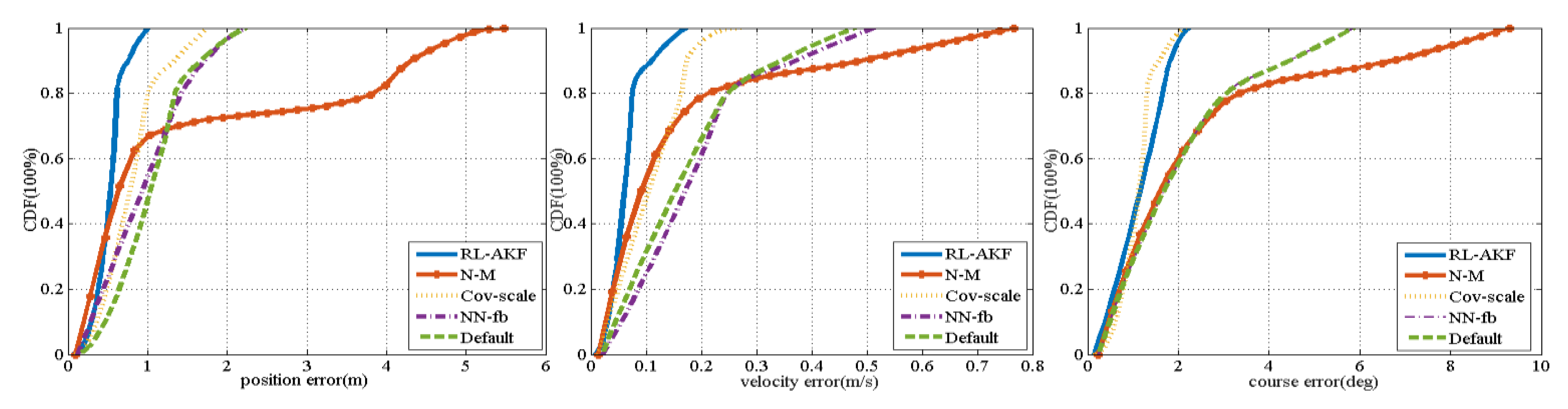
Figure 8 depicts the cumulative probability distribution of various errors of the process noise covariance matrix learnt from July 10 and tested on the July 17 data. The experimental results show that the positioning error is still at the sub-meter level. The forward and rightward position errors are substantially flat. Figure 9 and Figure 10 demonstrate detailed positioning results under a section of the path in the positioning process. The blue triangle periods simulate the GNSS signal loss by not performing the GNSS measurement update. It can be seen from the figure that our integrated navigation algorithm has strong positioning robustness for GNSS hopping, vehicle turning, and long-term GNSS loss.

Figure 11 and

Table 6. Accuracy comparison on the 17 July test data.

Item	RL-AKF	N-M	Cov-scale	NN-fb	Default
p_67%(m)	0.5959	0.9847	0.9174	1.2035	1.2309
p_90%(m)	0.7558	4.3011	1.3387	1.7144	1.6722
p_rms(m)	0.6075	2.8496	0.9978	1.4251	1.3425
v_67%(m/s)	0.0703	0.1354	0.1371	0.2145	0.2034
v_90%(m/s)	0.1105	0.4911	0.1709	0.3725	0.3459
v_rms(m/s)	0.0741	0.6116	0.1341	0.2457	0.2478
c_67%(deg)	1.4520	2.3270	1.2643	2.3326	2.3425
c_90%(deg)	1.8238	6.7497	1.5780	4.4513	4.4615
c_rms(deg)	1.6548	3.3338	1.2132	3.0215	3.0524

compare the navigation results using different algorithms on the July 17 test data. As can be seen from the experimental results, our proposed RL-AKF performs best overall. The NN-feedback algorithm has the weakest learning ability and finally performs as well as the default process noise covariance matrix. The positioning accuracy of the Nelder–Mead algorithm at 67% is better than the default process noise covariance matrix, but the position error at 90% diverges too much. The course error estimated by Cov-scale algorithm is slightly smaller than that of RL-AKF algorithm, but the latter still outperforms in position and velocity estimation.

To evaluate the robustness of our proposed RL-AKF on different time, we use the process noise covariance matrix learnt by the RL-AKF on July 10 to test with a completely new dataset collected on 17 July, and find that the RL-AKF still can obtain reasonable positioning accuracy, as Table 5 shows. The experimental results demonstrate that the process noise covariance matrix estimated with our proposed method can be used for integrated navigation for a rather long period of time with good accuracy.

3.5.2. Accuracy Comparison of Different GNSS Outage Periods

In the actual positioning scene, the GNSS outage moment is difficult to predict and the duration is uncertain. Therefore, we need the RL-AKF learnt process noise covariance matrix to be adaptive to different GNSS outage time periods. To evaluate the accuracy with different GNSS outage time periods, we compare the positioning error under the learnt covariance matrix and other algorithms with 10 s, 20 s, …, 60 s GNSS outage, separately. The error variations with different GNSS outage time periods are shown in

Table 7. Accuracy comparison with different GNSS outage periods.

Periods	RL-AKF	N-M	Cov-scale	NN-fb	Default
10s	0.6517	0.7724	0.8773	1.1024	1.0578
20s	1.9730	5.7627	2.4160	3.9617	4.2157
30s	5.1794	28.8819	7.2712	9.2458	9.6138
40s	8.3244	46.1954	11.8819	17.3697	16.3254
50s	14.9237	-	18.5435	25.2157	25.1732
60s	20.4279	-	24.7773	31.2648	32.2154

.

As can be seen from Table 7, the positioning error of RL-AKF is nearly quadratic in relation to the GNSS outage time. The process noise covariance matrix learnt by the Nelder–Mead algorithm causes a rapid divergence of positioning errors when the GNSS outage time lasts longer. The Cov-scale algorithm can fit the inherent noise parameters of the sensor device to a certain extent and reduce the positioning error. However, on the whole, the RL-AKF can reasonably learn process noise covariance matrix and perform better than the comparative methods under various GNSS outage situations.

3.5.3. Accuracy Comparison of GNSS/INS/ODO System

Depending on the device and the actual positioning scenario, the number and the types of measurement used in the integrated navigation system may also differ. We hope that the process noise covariance matrix learnt from the GNSS/INS system can also be robust to various integrated navigation schemes.

Odometers have recently received more and more attention in the area of integrated navigation by providing reliable and low-noise velocity measurements. During the GNSS outage time, the odometer can still provide reliable measurement updates for the Kalman filter.

We compared the accuracy of GNSS/INS/ODO integrated navigation with the process noise covariance matrix learnt from the GNSS/INS system. The accuracy comparison is shown in Figure 12 and the statistical performance is listed in

Table 8. Accuracy comparison with different methods of GNSS/INS/ODO integrated navigation system.

Item	RL-AKF	N-M	Cov-scale	NN-fb	Default
p_67%(m)	9.3911	26.4577	14.5501	21.4873	20.4578
p_90%(m)	28.7662	34.2566	27.2024	30.2443	31.2548
p_rms(m)	14.9426	29.9687	18.0201	25.1547	24.2454
v_67%(m/s)	0.1272	0.1427	0.0998	0.1143	0.1025
v_90%(m/s)	0.1853	0.1987	0.1367	0.2156	0.2438
v_rms(m/s)	0.1249	0.1723	0.0991	0.1467	0.1587
c_67%(deg)	0.7566	1.2543	0.9635	1.0259	1.2578
c_90%(deg)	1.0196	1.7628	1.7159	1.5946	1.5687
c_rms(deg)	0.6920	1.5324	1.1488	1.2913	1.2744

. To evaluate the accuracy with a rather long period of GNSS outage, we increased the GNSS outage time to 300 s.

As can be seen from Table 8, the velocity error using the default covariance matrix and Cov-scale is smaller than that using the covariance matrix learnt by the RL-AKF method. However, the latter can obtain less position and course error than other algorithms. We infer that with the Q matrix learnt from GNSS/INS integrated navigation it is difficult to accurately represent the relative relationship between the odometer measurement and the predicted velocity obtained from the inertial navigation, while the odometer speed using the default covariance matrix can provide more accurate velocity estimation. However, the learnt covariance matrix is much better for the course and position estimation. That may be the reason why the overall performance of the covariance matrix learnt by the RL-AKF method is better. Nevertheless, we guess that using our proposed method to estimate the process noise covariance matrix of GNSS/INS/ODO will achieve better performance. Considering the limited space, we will not repeat it here.

3.5.4. Accuracy Comparison of GNSS/INS/NHC System

Non-Holonomic Constraint (NHC) is another method that has been widely used as a measurement update for the vehicle navigation system based on the Kalman filter, which assumes that the vehicle’s velocity in the carrier coordinate system will always be zero in the rightward and upward direction. In this section, we compared the performance using different estimation methods with an extra NHC integrated navigation module. The experimental results are shown in Figure 13 and listed in

Table 9. Accuracy comparison with different methods of GNSS/INS/NHC Integrated Navigation System.

Item	RL-AKF	N-M	Cov-scale	NN-fb	Default
p_67%(m)	12.7463	34.2574	17.7241	27.8423	26.2548
p_90%(m)	22.4210	40.5821	39.1731	40.2518	41.2658
p_rms(m)	15.3380	36.2158	20.9373	33.4861	32.2581
v_67%(m/s)	0.1668	0.2156	0.1730	0.2186	0.2027
v_90%(m/s)	0.4637	0.2542	0.2198	0.2437	0.2256
v_rms(m/s)	0.2370	0.2467	0.1675	0.2259	0.2122
c_67%(deg)	0.6523	1.2957	1.1481	1.2999	1.3284
c_90%(deg)	0.9581	1.9524	1.7248	1.7654	1.8766
c_rms(deg)	0.7211	1.4755	1.2218	1.5284	1.4657

.

The rule shown in Table 9 is basically similar to Table 8. As the NHC provides a new measurement update for the velocity, the velocity estimation using the RL-AKF is slightly worse than other methods because the process noise covariance matrix used for RL-AKF is learned from the GNSS/INS integrated navigation scheme. Since the confidence of NHC measurements is less than that of the ODO, the accuracy of velocity using the NHC constraint is not obvious. The overall accuracy using our proposed RL-AKF method is still better than the comparative methods.

4. Discussions

Different from the measurement noise covariance matrix, the influence of the process noise covariance matrix on the positioning results is not easy to quantitatively evaluate after several rounds of iterations. Therefore, the feedback correction algorithm is not suitable for estimating the process noise covariance matrix. Inspired by the strong automatic exploitation of reinforcement learning, we introduce the reinforcement learning into the process noise covariance matrix estimation, which can avoid the direct gradient back propagation operation of position error to the process noise covariance matrix.

From the above-mentioned experiments, we can find that the main advantages of our proposed algorithm include the following three aspects. (1) Using the RL-AKF method can obtain a more accurate position, velocity and course estimation compared with other state-of-the-art methods. (2) The process noise covariance matrix learnt by the RL-AKF method can keep the validity for a certain period of time, which avoids continuous front and back data transmission. (3) The covariance matrix estimated by the RL-AKF method can adapt to various measurements for Kalman Filter, which is suitable for complex and dynamic practical application environment.

As concerns (1), during the absence of any other measurement assistance, the 10 s error of pure inertial navigation is 0.6517m. Taking the average road speed of 36km/h, that is, 10 m/s, as the standard, it can be obtained that the overall position error of the vehicle under the pure inertial navigation system will not exceed a standard lane after 400 m driving, and the lateral position deviation is even smaller. With the help of the odometer, the displacement of the vehicle after running 3000 m shall not exceed 10 m. At this time, the integrated navigation can reasonably meet the high-accuracy and continuous positioning needs in the special areas, such as in the long tunnel and high-density forest area.

The process noise covariance matrix will change with the temperature. However, the temperature will not change much for a short period of time. Then, the covariance matrix will not have a great change either since it represents the inherent performance of the sensor device. Therefore, after an effective estimation of the process noise covariance matrix for a specific device is made by this algorithm, the quadratic estimation is not needed in the subsequent navigation process. It is not necessary to estimate the process noise covariance matrix in real-time. Our presented algorithm is energy-efficient, which transmits sensor data to the background for learning on demand and returns the prediction results to the embedded platform.

In the actual positioning scene, other observational measurements such as odometer, empirical measurements such as non-holonomic constraints, and opportunistic measurements such as zero velocity detection may be applied to Kalman filter. The process noise covariance matrix obtained by this algorithm can well represent the prediction performance of navigation state in the inertial navigation phase. This makes the RL-AKF algorithm available for occasional increase or decrease of different measurements in Kalman filter.

However, RL-AKF algorithm also has some limitations. While the robustness of this algorithm greatly reduces the training frequency of RL part, it is undeniable that this algorithm takes a long time for once training, which is mainly caused by the computational overhead of integrated navigation itself and the complexity of the reward definition. In addition, the algorithm requires the integrated navigation device to store 200 s of IMU and GNSS data, which brings additional storage overhead to the device. These two aspects will be optimized and improved in our future work.

5. Conclusions

In this paper, we introduce the adaptive estimation of the process noise covariance matrix for the Kalman filter based on the strong automatic exploitation of reinforcement learning. By taking the integrated navigation system as the environment, and the opposite of the current positioning error as the reward, the RL-AKF algorithm uses the deep deterministic policy gradient to obtain the most optimal state estimation and the process noise covariance matrix from the continuous action space. The RL-AKF can significantly improve the positioning performance of the integrated navigation when the GNSS signal is not available. Our approach will not affect the real-time performance of integrated navigation since the training process can be independently run on the cloud platform. Moreover, the RL-AKF needs only 0.57 MB of additional storage space and requires data transmission operations between the embedded platform and cloud platform only after the embedded platform issues a new training request. The experimental results demonstrate that using the process noise covariance matrix estimated by our proposed algorithm can obtain accurate position estimation, which is robust under different times, different GNSS outage time periods and using different integration navigation fusion schemes.