Article

Super-Resolution-Based Snake Model—An Unsupervised Method for Large-Scale Building Extraction Using Airborne LiDAR Data and Optical Image

by
Thanh Huy Nguyen
1,2,*,
Sylvie Daniel
2,
Didier Guériot
1,
Christophe Sintès
1 and
Jean-Marc Le Caillec
1
1
IMT Atlantique, Lab-STICC, UMR CNRS 6285, F-29238 Brest, France
2
Department of Geomatics, Université Laval, Quebec City, QC G1V 0A6, Canada
*
Author to whom correspondence should be addressed.
Remote Sens. 2020, 12(11), 1702; https://doi.org/10.3390/rs12111702
Submission received: 18 April 2020 / Revised: 20 May 2020 / Accepted: 22 May 2020 / Published: 26 May 2020
(This article belongs to the Special Issue 3D City Modelling and Change Detection Using Remote Sensing Data)

Abstract

:
Automatic extraction of buildings in urban and residential scenes has become a subject of growing interest in the domain of photogrammetry and remote sensing, particularly since the mid-1990s. Active contour model, colloquially known as snake model, has been studied to extract buildings from aerial and satellite imagery. However, this task is still very challenging due to the complexity of building size, shape, and its surrounding environment. This complexity leads to a major obstacle for carrying out a reliable large-scale building extraction, since the involved prior information and assumptions on building such as shape, size, and color cannot be generalized over large areas. This paper presents an efficient snake model to overcome such a challenge, called Super-Resolution-based Snake Model (SRSM). The SRSM operates on high-resolution Light Detection and Ranging (LiDAR)-based elevation images—called z-images—generated by a super-resolution process applied to LiDAR data. The involved balloon force model is also improved to shrink or inflate adaptively, instead of inflating continuously. This method is applicable for a large scale such as city scale and even larger, while having a high level of automation and not requiring any prior knowledge nor training data from the urban scenes (hence unsupervised). It achieves high overall accuracy when tested on various datasets. For instance, the proposed SRSM yields an average area-based Quality of 86.57% and object-based Quality of 81.60% on the ISPRS Vaihingen benchmark datasets. Compared to other methods using this benchmark dataset, this level of accuracy is highly desirable even for a supervised method. Similarly desirable outcomes are obtained when carrying out the proposed SRSM on the whole City of Quebec (total area of 656 km2), yielding an area-based Quality of 62.37% and an object-based Quality of 63.21%.

1. Introduction

1.1. Motivation

Automatic and accurate extraction of building footprints from urban scenes using remote sensing data has become a subject of growing interest for a wide range of applications, such as urban planning [1], city digital twin construction [2], census studies [3], and disaster and crisis management, namely earthquake and flood [4,5].
This research work presents an effective solution for extracting buildings from urban and residential environments in a large scale. Such a task plays an important role in the context of flood risk anticipation, which is asserted with a particular importance in the province of Quebec, Canada [6]. Such a context requires accurate and regularly updated building footprint location and boundary, which enable the extraction of further essential structural and occupational characteristics of buildings (e.g., first floor, basement openings). In addition, the scalability of this solution—i.e., the ability to maintain its effectiveness when expanding from a local area to a large area [7]—is crucially important considering the scale of the study (i.e., at the scale of the province of Quebec).
The nature of urban and residential environments can be very complex, where buildings can be found with various sizes, colors and shapes, within urban areas of different density and vegetation coverage. Such complexity is problematic for developing a large-scale building extraction solution. Indeed, a number of studies have been reported over the years with relatively significant results by assuming building shapes [8,9,10], enforcing geometrical constraints [11], or limiting on specific urban areas. However, such assumptions and constraints limit the scalability of the building extraction method, in particular over large areas composed of numerous and complex structures. Based on these premises, it is necessary that such a solution is (i) versatile—applicable on different urban scenes without relying on predefined assumptions, constraints, or prior knowledge about the involved scenes and buildings; (ii) highly accurate; (iii) and easily scalable over large areas with a relative computational simplicity. To the best of our knowledge, such a solution has not yet been found.

1.2. Literature Review

A large number of building extraction methods have been reported over the last few decades, particularly with the emergence of Light Detection and Ranging (LiDAR) systems since the mid-1990s [12]. However, this task remains very challenging due to various difficulties. For instance, many works [13,14,15,16] have been carried out using aerial and satellite imagery. They face many problems due to occlusions, poor contrasts, shadows, and disadvantageous image perspectives [17]. Since height changes allow distinguishing urban objects more effectively than the spectral and textural changes from optical images, numerous works [18,19] proposed to exploit 3-D information from LiDAR to extract buildings. However, these methods usually face problems of misclassification of vegetation as buildings [20]. In addition, the accuracy of extracted boundaries can be compromised due to the LiDAR point cloud sparsity [21]. Therefore, many researchers have developed a consensus strategy to use multisource data in order to increase the building detection rate. Hence, a number of studies [22,23] focusing on the integration of LiDAR and optical imagery data have been reported. They succeed at improving the building extraction accuracy, compared to the use of individual data source [24]. However, such an approach of integrating multisource data can be problematic due to data misalignment [25].
The International Society for Photogrammetry and Remote Sensing (ISPRS) Working Group II/4 “3D Scene Reconstruction and Analysis” provided a taxonomy for methods submitted to the urban object detection benchmark test [26], based on their processing strategy. Some of the methods are categorized as supervised methods requiring training data from LiDAR point cloud or optical image, such as Niemeyer et al. [27] and Chai [28]. They provided two of the highest accuracy methods submitted to the ISPRS Vaihingen benchmark. Many other methods are categorized as model-based methods, as they rely on an explicit model or a set of predefined rules on the appearance of the buildings in the data. For instance, Bayer et al. [29] proposed a segmentation-based method involving multiple thresholds applied on the Digital Surface Model (DSM) and Normalized Difference Vegetation Index (NDVI) to separate buildings and trees. Similarly, Grigillo and Kanjir [30] proposed two versions of a model-based method based on rule-set classifiers on image pixel colors and NDVI. However, the selection of such thresholds and rules is strongly scene-dependent.
Active contour model [31], or colloquially known as snake model, is an object boundary extraction technique widely used in computer vision and image processing [32] (Ch. 5). Snakes or active contours are energy-minimizing curves, defined within an image domain, that move under the influence of internal forces within the curve itself and other external forces. This technique has also been intensively studied to extract buildings from urban and residential areas. In contrast to other approaches mentioned above, it provides a building extraction solution without prior knowledge about the image and the building shapes. Moreover, this technique provides a computational simplicity and an advantageous flexibility allowing external constraint forces introduced by the user. These characteristics show that snake model is suitable to be developed into a large-scale solution that fits our purposes.

1.3. Snake Model-Based Related Works

Guo and Yasuoka [33] used snake model with balloon force to extract buildings using high-resolution satellite images and height data. Peng et al. [34] focused on improving the stability of snake convergence on aerial images. Kabolizade et al. [35] proposed a snake model using imagery data coupled with a DSM generated from LiDAR data. This model involves the minimization of variances of height and gray level between snake points. Consequently, it requires height information for every pixel of the image; in other words, the DSM must be of the same size and resolution as the optical image. Such a requirement is problematic since LiDAR datasets usually have subsampled spatial resolution compared to the aerial imagery, yet a simple interpolation of height data could be unreliable. In contrast, Ahmadi et al. [36] proposed a geometrical snake model to detect building boundaries from aerial images, without height information or manual initial points. However, this model requires a priori gray levels of buildings and ground and uses them as training data to attract the snakes toward desired buildings. Consequently, it yields a high number of misdetected buildings when they consist of untrained color. Additionally, it does not work well with the building roofs having varying gray levels. Fazan and Dal Poz [37] proposed a method involving exhaustive searches for rectilinear building corners in the optical images, based on the basic snake model optimized by dynamic programming. Yet this method depends heavily on initial points to have decent results. Snake models have also been demonstrated as an efficient tool to refine the public Geographic Information System (GIS) building footprints [38]. The improved footprints are then fed into Convolutional Neural Networks (CNNs) as labeled data for the building segmentation.
Our previous work [39] presented an unsupervised and automatic snake model to extract buildings from optical imagery. It is carried out based on a snake model operating on optical image, initialized and enhanced by integrating with LiDAR data. This snake model involves a novel external energy term computed based on the shape similarity between the snake and the projected LiDAR building boundary. Such an energy term encourages the snake to maintain a shape similar to the building boundary extracted from LiDAR data, while moving under the attractions of salient features provided by optical image. In contrast to the snake models mentioned above, this method succeeds at extracting buildings in various difficult cases, e.g., building roof with similar color to its background, gable-roof houses, or varying-color roof buildings. Without any human intervention or training data, it is able to achieve higher accuracy than existing snake models and many existing building extraction methods such as [25,40,41] on multiple test areas (see [39] for the full assessment). Nevertheless, similarly to other existing snake models, it still concedes a number of challenges, namely its sensitivity against image noise and undesired details and the hyperparameter tuning for snake model in a large scale.
While there is not currently any effective solution regarding the former problem (i.e., snake sensitivity) when using optical imagery, the latter problem (i.e., hyperparameter tuning) has been partially addressed by Marcos et al. [42] with a deep learning-based approach. It involves using a CNN to learn the characteristics of the snake model elements, i.e., parameters and energy terms, from training optical images and associated ground truth polygons. The CNN-inferred parameters and energy terms enabled this snake model to achieve higher accuracy compared to other deep learning-based building extraction methods. However, the main drawback of this method is that it involves every image patch—each one containing a building—to have the same size, i.e., 512 × 512 pixels, for both the training dataset and the test dataset. This means that all the concerned buildings (training and testing) must have similar size in order for the CNN to learn and predict the parameters and energy terms. In other words, in order to resolve the snake parametrization problem, this approach proposed by Marcos et al. [42] requires the building size consensus. This requirement affects directly the method reproducibility on buildings of different sizes. Consequently, such a CNN-based snake parametrization approach is not scalable for large areas consisting of buildings of various sizes.

1.4. Contribution

The objective of this research work is to develop a large-scale automatic and accurate building extraction based on snake model, fulfilling the following requirements. Firstly, such an effective snake model would require an automatic and reliable initialization. Secondly, the snake model should not be sensitive to noise and details in the image. Thirdly, the snake model parameters should be relevant when applied to a large extended area with buildings of various shapes, sizes, and colors. While the first requirement is addressed by using the boundaries preliminarily extracted from LiDAR point cloud, the second and the third remain very challenging. In this regard, the contributions of this work are threefold:
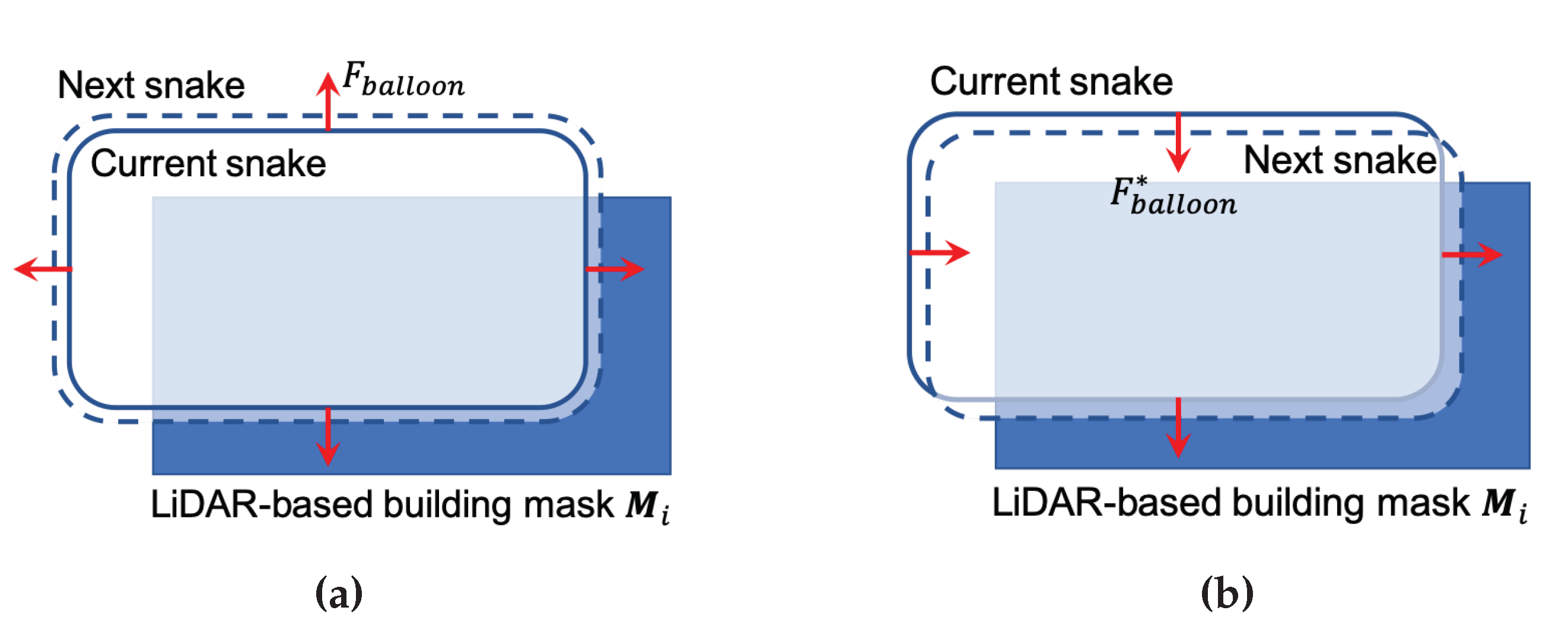
  • We propose an effective solution to compute the external energy for the snake model—which is initialized by the LiDAR-based boundaries. Such a solution enables the snake model to be insensitive to image noise and details, as well as easing the snake model parametrization. In addition, this snake model involves an improved balloon force that behaves adaptively by either shrinking or inflating the snake (as opposed to the classic balloon force that always inflates it).
  • In order to build a reliable foundation for this novel snake model, a super-resolution process is proposed to reliably improve the LiDAR point cloud sparsity. Such a sparsity issue has been problematic to building extraction methods using LiDAR data, including snake models.
  • Lastly, we present a comprehensive performance assessment of the proposed SRSM on two different geographical contexts, namely Europe (with the Vaihingen benchmark dataset) and North America (with the Quebec City dataset). Such contexts involve various differences in terms of compactness, density, and regularity of urban areas [43], demonstrating the scalability and versatility of the proposed method.
Together, these elements constitute a large-scale automatic and unsupervised building extraction method, which achieves high thematic and geometrical accuracy when tested on various urban scenes.

1.5. Paper Organization
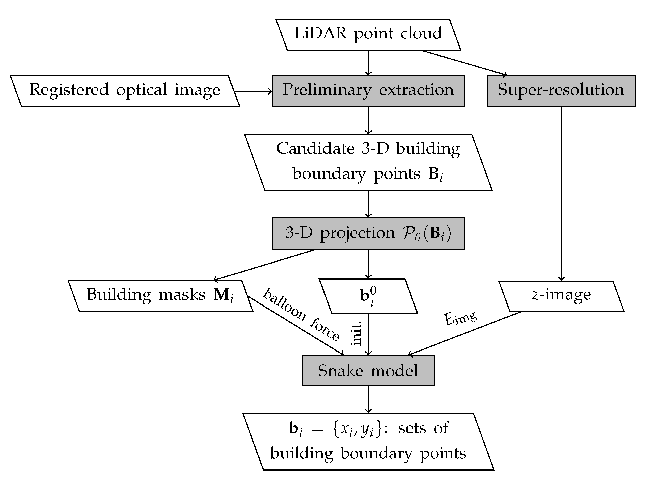
This paper is structured as follows: this section has been devoted to an introduction to the building extraction research topic, our motivation, and a literature review of the related works. The contributions of this research work have also been summarized. Section 2 presents the proposed method. Then, multiple assessments on the performance of the SRSM involving various study areas and datasets are carried out in Section 3. Next, Section 4 brings the discussions on the relevance of the proposed SR, then on the SRSM results, and lastly on the impact of the snake model parametrization. Finally, Section 5 provides conclusions and perspectives of this work.

2. Proposed Method

This paper presents a novel unsupervised building extraction method, built around the Super-Resolution-based Snake Model (SRSM). Figure 1 depicts the flowchart of the proposed method. It employs predominantly the LiDAR data, with additional information from the optical image in order to remove vegetation. First, the SRSM is automatically initialized by the preliminary candidate building boundaries extracted from the LiDAR point cloud. This extraction process is carried out as presented in [39]. It relies on an elevation thresholding, a proximity regrouping, and a convex hull detection. The ground elevation value is determined by a DTM, generated using the method proposed by [44]. This process is also similar to other research works such as [25,45]. Since LiDAR-based building extraction can be difficult due to nearby vegetation [46], this process also involves a vegetation removal based on the Normalized Difference Vegetation Index (NDVI) derived from an optical image. As the two data sources are used jointly, a registration is necessary in order to avoid misalignment problems. This registration can be carried out a priori (i.e., data acquisition using the same platform) or a posteriori [47,48]. It aims to estimate the transformation model, allowing reducing the misalignment between the two datasets. The 3-D building boundary points extracted from the LiDAR point cloud are denoted by B i , where i represents the building index. The registration results in a set of transformation model parameters θ , which is then used for the projection of the 3-D building boundary points B i onto the image space, denoted by P θ ( B i ) . Then, they are used as initial points (denoted by b i 0 ) for the snake model, as well as to generate the building masks (denoted by M i ) used in the balloon force. The SRSM operates on high-resolution LiDAR-based z-images generated by a super-resolution process. It also involves an improved balloon force model based on the building masks M i . The resulting building boundary is denoted by b i .

2.1. Mathematical Formulation

An active contour or a snake, is a dynamic curve x ( s ) = ( x ( s ) , y ( s ) ) , where s [ 0 , 1 ] is the normalized arc length, defined within an image domain that is deformable under the influence of internal and external forces. The behaviors of the snake are governed by an energy function defined as follows,
E snake = 0 1 ( E int ( x ( s ) ) + E ext ( x ( s ) ) ) d s
with E int ( x ( s ) ) = 1 2 α x s 2 + β 2 x s 2 2
and E ext ( x ( s ) ) = E img ( x ( s ) ) + E con ( x ( s ) )
where E int and E ext , respectively, represent the internal and external energy terms. The internal energy term relates to the amount of stretch and curvature of the snake, respectively controlled by weighting parameters α and β . Small values of α and β , respectively, encourage short and smooth contours and vice versa. The external energy E ext is composed of the forces due to the image itself E img and other constraint forces E con . The external image-based energy E img involving salient features of the image, i.e., lines, edges, and terminations (i.e., line segment end-points, corners) is formulated as follows,
E img = w l i n e E l i n e + w e d g e E e d g e + w t e r m E t e r m
where w l i n e , w e d g e , w t e r m are the weights of the respective salient features. Mathematical formulation of these energy terms [31] are provided in Appendix A.
A snake that minimizes E snake described by Equation (1) must satisfy the following Euler equation,
α × x 2 s 2 + β × x 4 s 4 + E ext = 0
In order to solve Equation (3), the snake is made dynamic by regarding x as a function of time t as well as of the arc length s. Then, the partial derivative of x with respect to t is then set equal to the left-hand side of Equation (3), as follows,
x t = α × x 2 s 2 β × x 4 s 4 E ext
As x ( s , t ) stabilizes, the partial derivative term x / t vanishes and a solution for Equation (3) is obtained. A numerical approach for Equation (4) can be carried out by discretizing the equation and solving the discrete problem iteratively [31].
External constraint forces are added to the snake energy function in order to guide it toward or away from a particular feature, as well as addressing snake problems such as initialization, convergence, and robustness against noise. In this regard, Xu and Prince [49] proposed Gradient Vector Flow (GVF) to improve the traditional snake model by allowing more flexible initialization and encouraging its convergence to boundary concavities, as well as improving its robustness. GVF field is defined as the vector field v ( x , y ) = ( u ( x , y ) , v ( x , y ) ) that minimizes the energy functional
E GVF = μ GVF ( u x 2 + u y 2 + v x 2 + v y 2 ) + | f | 2 | v f | 2 d x d y
with μ GVF being a controllable smoothing term and f representing external forces from Equation (3), i.e., f ( x , y ) = E ext . Using [50] the GVF field v can be found by solving
μ GVF 2 u ( u f x ) ( f x 2 + f y 2 ) = 0 μ GVF 2 v ( v f y ) ( f x 2 + f y 2 ) = 0
where 2 is the Laplacian operator. The Euler equations (6) can also be solved by regarding u and v as functions of time,
u t = μ GVF 2 u ( x , y , t ) [ u ( x , y , t ) f x ( x , y ) ] · [ f x ( x , y ) 2 + f y ( x , y ) 2 ] v t = μ GVF 2 v ( x , y , t ) [ v ( x , y , t ) f y ( x , y ) ] · [ f x ( x , y ) 2 + f y ( x , y ) 2 ]
Once computed v ( x , y ) replaces the potential force E ext in the dynamic Equation (4), yielding
x t = α × x 2 s 2 β × x 4 s 4 + v
This equation is solved similarly as the traditional snake model, i.e., by discretization and iterative solution. The parametric curve solving the above dynamic equation is thus called a GVF snake.
Cohen [51] proposed an inflation term as an external force, known as balloon model, as follows,
F balloon = κ × n ( s )
where κ is the magnitude of the force and n ( s ) stands for the normal unitary vector of the curve at x ( s ) . This model mimics the inflation of a balloon by continuously pushing the snake points outward. Thus it prevents the snake from shrinking into a single point.

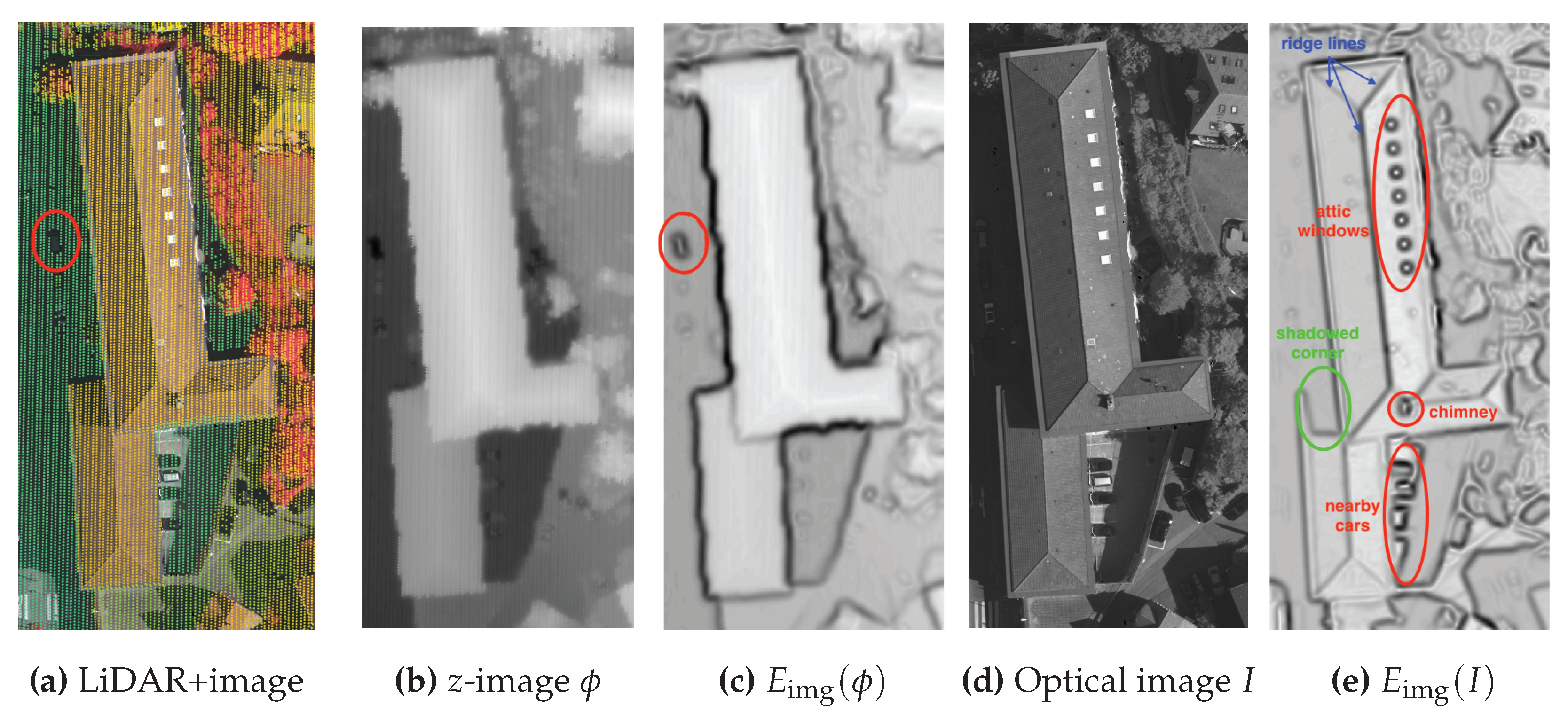
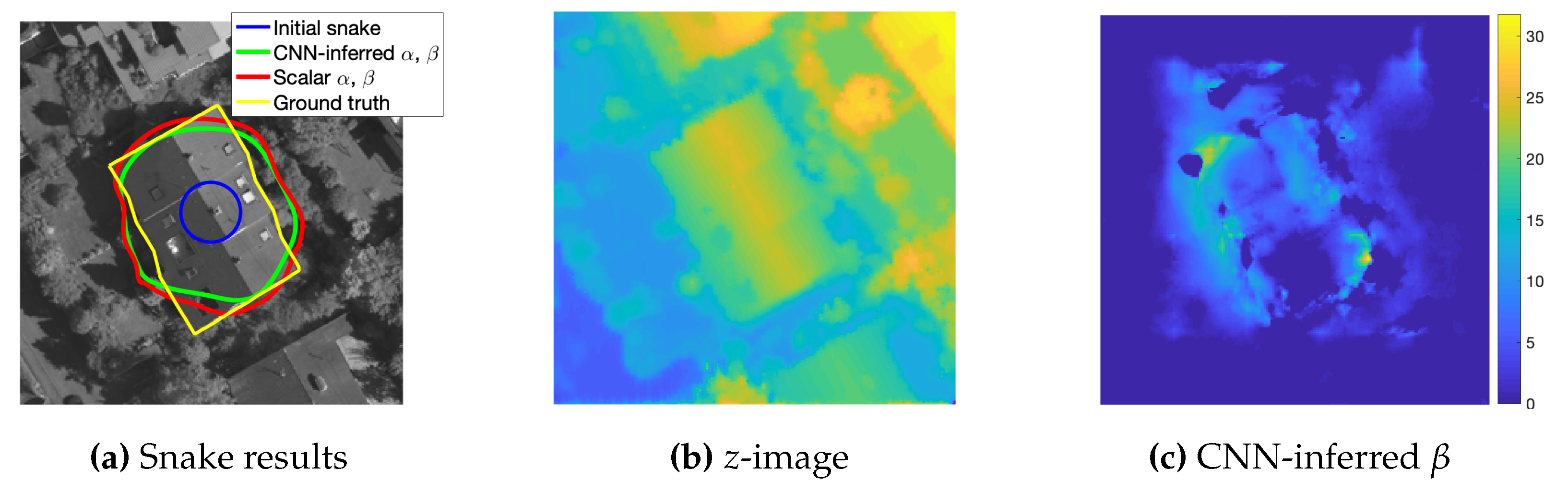
2.2. Proposed Z-Image-Based Energy Term

Despite the recent developments, the existing snake models still struggle to yield a satisfactory reproducibility in complex environments. Such low reproducibility stems from a number of reasons. For instance, these environments can be composed of complex structures such as multiplanar roof buildings which can also be shadowed or occluded by trees. For a multiplanar roof building, different roof planes can have different shades, causing ridge lines (i.e., the intersection lines between the different planes) exhibiting high-gradient values in the image-based energy term. In addition, the performance of the snake model on optical images can be affected by image small details, namely roof objects (like chimneys, attic windows), cars, trees, etc. There are also possible null-valued pixels on the orthoimage. Consequently, if a building involves these unwanted elements, then the snake model would be drawn toward them. Hence, the resulting performance on delineating such a building would decrease significantly. Fortunately, these problems relate directly to the use of the optical image. Therefore, we propose to operate the snake model on the z-image derived from LiDAR data. This approach allows the snake model to focus only on the most salient features in a z-image, i.e., height changes involving off-terrain objects such as buildings and trees.

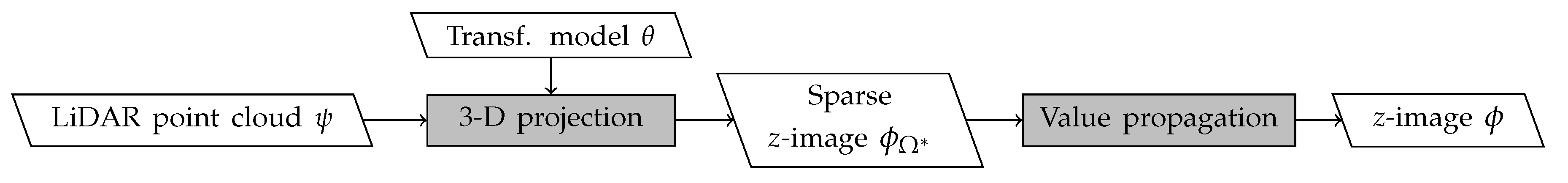
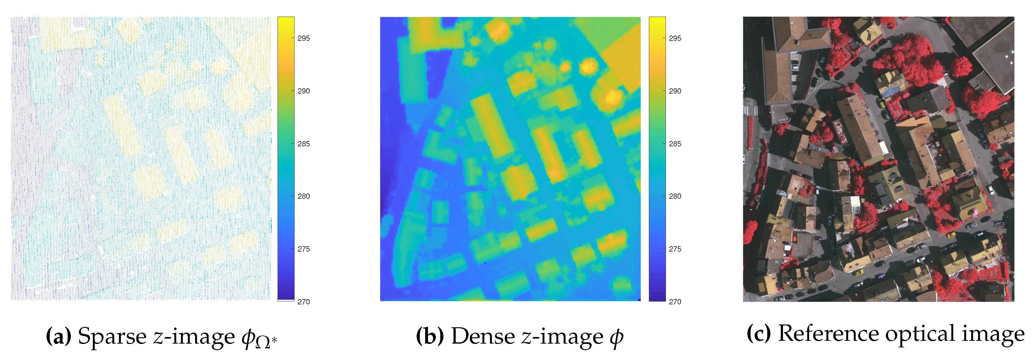
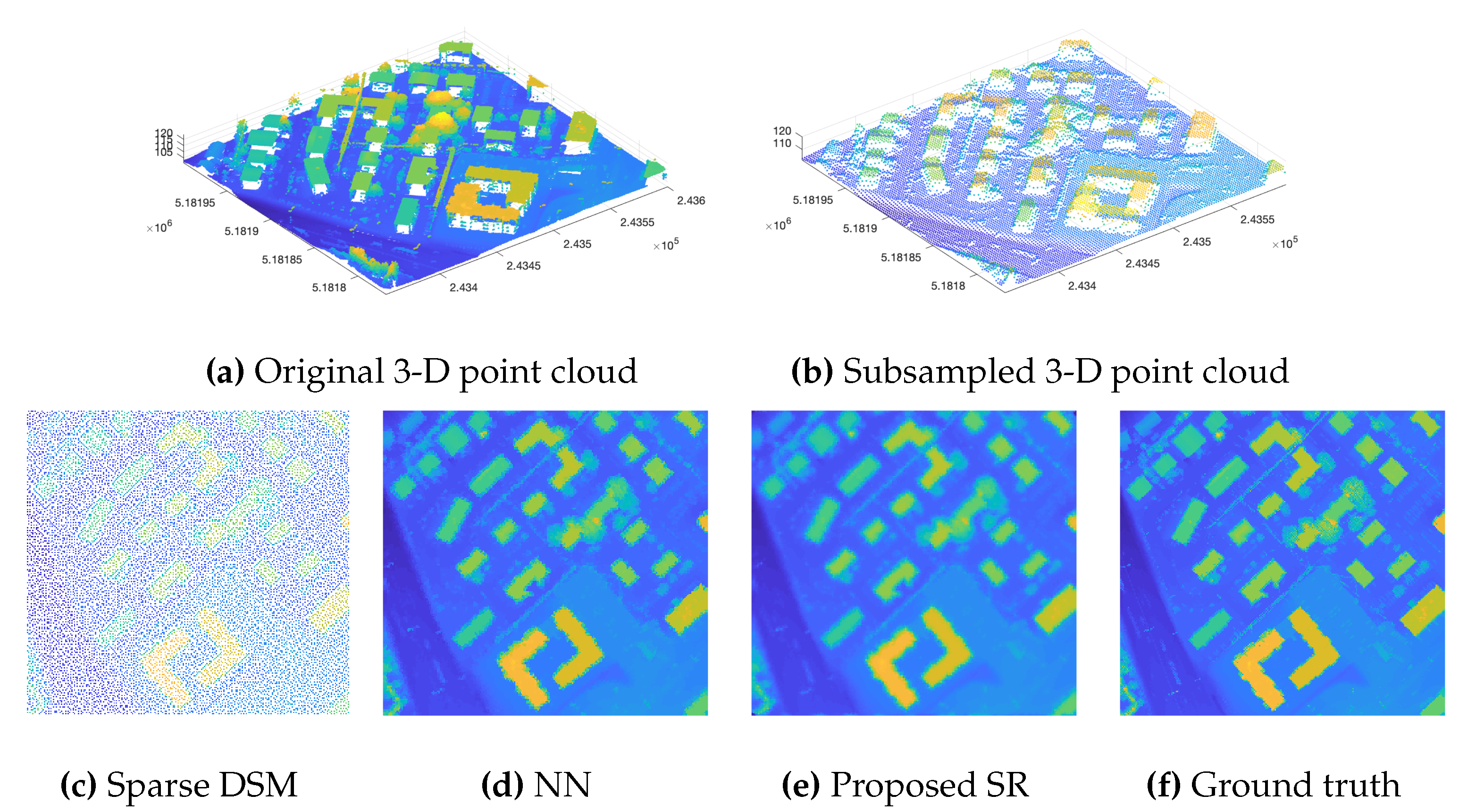
2.2.1. Generation of Z-Image by the Super-Resolution of LiDAR Data

The accuracy of a building extraction method using LiDAR data is usually compromised by the sparsity problem [21]. Therefore, we propose a process dedicated to the projection and propagation of LiDAR data onto the image space in order to augment its spatial resolution. Such a process is called super-resolution (SR), and it is illustrated by the flowchart in Figure 2. It consists in generating a z-image that contains the altitude values derived from the LiDAR 3-D point cloud. Such an image has the same size and resolution as the optical image. The inputs of the SR process are the LiDAR point cloud, a set of transformation model parameters, the frame of reference, and the size of the optical image. The LiDAR 3-D point cloud is denoted by ψ R m × 3 where m is the number of points. Each point has three spatial coordinates ( x , y , z ) . We also use ψ z R m for the column of altitude values. The z-image is denoted by ϕ R n x × n y , where n x and n y are, respectively, the number of rows and columns. During the SR process, ϕ is vectorized into a column vector of n = n x × n y elements. The set of transformation model parameters θ results from the registration [48]. It aims to define the projection of 3-D points onto the image space.
(a)
Projection of LiDAR 3-D points
The first step of the SR process consists in projecting the LiDAR 3-D points onto the z-image space using the transformation model parameters θ . As the LiDAR point cloud is subsampled compared to the optical image, such a projection leads to a sparsity effect on the z-image ϕ . Here, we use Ω * and Ω to denote, respectively, the subset of the pixel indices in the z-image ϕ , having or not a projected altitude value. In other words, ϕ Ω * denotes the sparse z-image or the subvector containing the pixels of projected altitude value, whereas ϕ Ω denotes the subvector containing the null pixels. The dimensions of ϕ Ω * and ϕ Ω , respectively, are m × 1 and ( n m ) × 1 . As such, ϕ = ϕ Ω Ω * is the vector containing all pixels, i.e., the whole z-image. The projection is mathematically presented as follows,
ϕ Ω * = P θ ( ψ z )
where P θ is the 3-D projection associated with the transformation model parameters θ . The x- and y-coordinates of the LiDAR 3-D points are used to locate the pixels in the z-image associated with such points. Next, the projected values indexed by Ω * will be propagated to their neighboring pixels (which are indexed by Ω ).
(b)
Propagation of the projected values
Our SR approach is inspired by the work of Castorena et al. [52] on the fusion of terrestrial LiDAR data with optical imagery. It involves reconstructing a sparse depth map by minimizing the sum of its squared directional gradients (SSDGs). This approach relies on hypothetical characteristics of a depth map, which involve the magnitude and occurrence of depth discontinuities inside the depth map to be minimized. In an airborne nadir view context, their method shows good performance in propagating elevation values across homogeneous regions. However, in elevation-discontinued transitioning regions, e.g., near the edges of a building, the propagated elevation values would be gradually flattened as a result of the minimized SSDGs. In other words, such hypothetical characteristics are not suitable in this context, where the off-terrain objects like trees and buildings always exhibit strong elevation discontinuities. Such discontinuities should be preserved during the value propagation process. Thus, an l 1 -norm term is added in our minimization approach. This preservation allows the resulting z-image to exhibit elevation changes as tight as possible compared to the scene reality.
The propagation of the projected values is carried out through the minimization of a cost function F ( ϕ ) , defined by Equation (11). It is composed of the SSDGs and a l 1 -norm term of the z-image ϕ , subjecting to the values previously projected from the point cloud (i.e., described by Equation (10)).
ϕ ^ = arg min ϕ x ϕ 2 2 + y ϕ 2 2 f SSDG ( ϕ ) + λ ϕ 1 F ( ϕ ) , subject   to   ϕ Ω * = P θ ( ψ z )
where · p stands for the l p -norm, x and y , respectively, represent the directional gradient operators along the x-axis and y-axis. The parameter λ > 0 controls the amount of the l 1 -regularization.
(c)
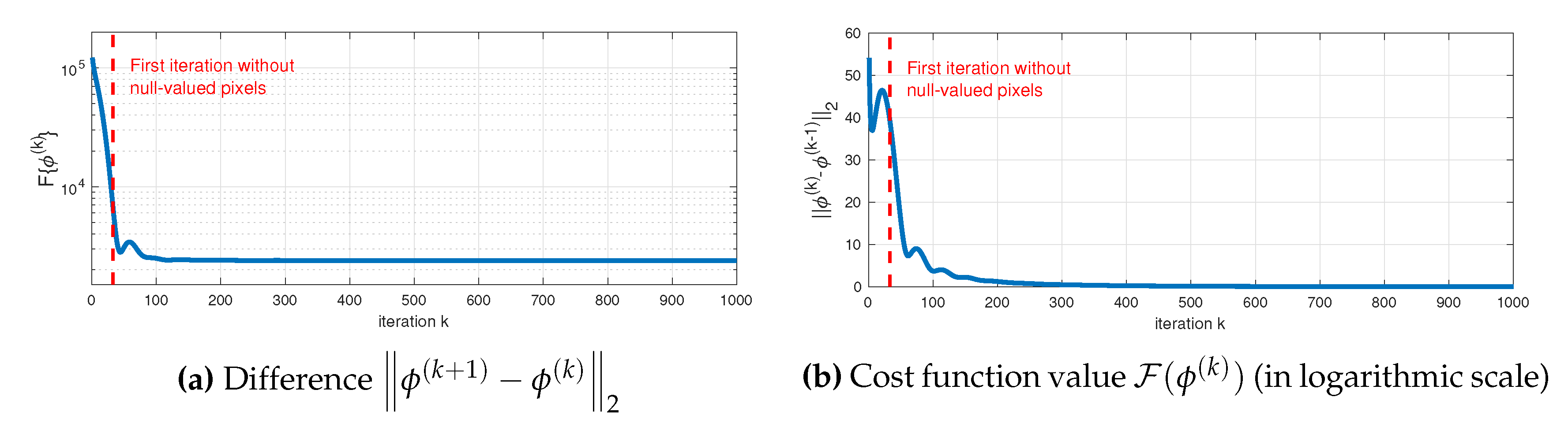
Propagation implementation
The minimization of the cost function described in Equation (11) is carried out using the Fast Iterative Shrinkage-Thresholding algorithm (FISTA) [53]. Its computational efficiency is adequate for solving large-scale problems, with a convergence rate of O ( 1 / k 2 ) , where k is the iteration counter. FISTA is significantly faster than standard gradient-based methods such as Iterative Shrinkage-Thresholding algorithms (ISTA). Full details on the implementation of the proposed SR process can be found in [48].
The convergence rate of the SR is illustrated in Figure 3. Figure 3a depicts the differences between the estimated z-images at consecutive iterations, i.e., ϕ ( k + 1 ) ϕ ( k ) 2 . The cost values F ( ϕ ( k ) ) through iterations are shown in Figure 3b. One can observe that the z-image has nearly converged into a stable solution after approximately four hundred iterations. Figure 4 shows the outcomes of the projection and the propagation of altitude values from the LiDAR data onto the optical image space. The value projection outcome is depicted by the sparse z-image ϕ Ω * (Figure 4a), whereas the value propagation outcome is shown by the dense z-image ϕ (Figure 4b). The pixel color of the sparse and dense z-images represents the surface elevation in meters. Figure 4c shows the reference optical image on the same urban scene, in order to assess visually the quality of the super-resolved z-image. It can be noted that the elevation of buildings and other objects (e.g., trees, cars, etc.) are well presented on the dense z-image (Figure 4b) and correspond to the information in the optical image. The proposed SR process is shown to achieve the purpose of augmenting the spatial resolution of the LiDAR point cloud. An assessment of the SR performance will be presented in Section 3.3.

2.2.2. The Z-Image Based Energy Term

Figure 5 depicts a comparison between the use of the z-image ϕ and the optical image (denoted by I) of a multiplanar roof building with several roof objects and nearby cars. Figure 5a reveals the LiDAR point cloud overlain on the optical image of the exemplified building. Figure 5b,c show, respectively, the z-image and the energy term computed from the z-image. Then, the optical image and the associated energy term are depicted, respectively, in Figure 5d,e. In Figure 5c,e, the grayscale reflects the value of the energy term E img . The dark pixels represent the low-energy pixels, whereas the bright pixels are the high-energy ones. By design, a snake is attracted to the dark pixels and will iteratively move toward them. Comparing the two energy terms (Figure 5c,e), it can be noted that the sources of attraction for the snake models, i.e., the dark pixels in the energy term, provided by the z-image are more relevant than the ones from the optical image. Indeed, the dark pixels from the energy term computed from the z-image E img ( ϕ ) (Figure 5c) are found mainly at the edges of the building, with a few exceptions caused by the nearby trees. There exists also one particular aberration which is circled in red on Figure 5c. It is caused by an absence of LiDAR points in this small region, as highlighted in the red circle in Figure 5a.
On the other hand, the dark pixels from the optical image-based energy term E img ( I ) (Figure 5e) stem from many undesirable artifacts, namely cars, attic windows, and chimneys found on this building roof. They are highlighted by the red circles on Figure 5e. By comparing Figure 5c,e, it can be noted that some of these artifacts do not exist or are much less visible on the z-image—due to their low elevation variations compared to the building-to-ground ones. In addition, the effect of shadow casting over a corner of the building—circled in green on Figure 5e—is also problematic to a building boundary extraction. Such an effect and problem do not exist in the z-image. We can also remark that this multiplanar roof building exhibits many ridge lines which also produce low values in the energy term. In reality, they are not false non-building details like trees or cars, but when focusing on the extraction of the building boundaries, they can be considered undesirable. These premises show that it is more relevant to carry out the snake model on the z-image than on the optical image.

2.3. Improved Balloon Force

As aforementioned, the classical balloon force is conceived to constantly push the snake outward based on its local curvature (Equation (9)). Such behavior becomes less relevant when addressing buildings with complex shape. Therefore, we propose to adapt the balloon force to push outward at some particular region and shrink inward at some others. Such adaptation is explained in the following. Using the 3-D building boundaries preliminarily extracted from LiDAR point cloud, a set of building masks M i can be created. Such masks are generated by projecting the 3-D building boundaries onto the image space and then determining the enclosed region inside the projected boundaries. Then, the adapted behavior is carried out through a signed magnitude matrix computed using the mask M i , as defined in Equation (12).
K i ( x , y ) = κ , i f ( x , y ) M i κ , i f ( x , y ) M i
with ( x , y ) being the coordinates of a point on the snake and κ being the force magnitude weight. As a result, the improved balloon force for a building i is given as in Equation (13),
F balloon , i * = K i ( x , y ) × n ( x , y )
where n stands for the normal vector of the curve at ( x , y ) .
Figure 6 depicts a schematic representation illustrating the proposed adaptation. It demonstrates how the snake behaves differently (i.e., either inflating or shrinking) based on its relation with the given LiDAR-based building mask. With the LiDAR-based building masks M i represented by the blue rectangle, the balloon force behavior (represented by the red arrows) is improved to shrink or inflate at different snake points.

3. Experimental Results

In this section, multiple performance evaluations are carried out. First, we introduce the building extraction accuracy metrics as well as the study areas and the datasets used in this work. Then, the performance of the SR process is evaluated. Next, a visual assessment between the snake models is also carried out. Lastly, the proposed SRSM is evaluated on various urban and residential scenes.

3.1. Building Extraction Accuracy Metrics

Multiple accuracy assessments, thematically and geometrically, are proposed to evaluate the performance of a building extraction method based on the ground truth boundaries.

3.1.1. Thematic Accuracy Metrics

Based on the evaluation methodology described by Rutzinger et al. [54], three metrics, namely Quality (Q), Completeness ( C p ), and Correctness ( C r ), are measured per-object and per-area. Particularly, the per-object evaluation involves either all objects regardless of their area or only the objects with an area larger than 50 m2. The three metrics are computed based on the count of true positive (TP), false positive (FP), and false negative (FN) elements between the extracted and the reference building boundaries from the ground truth. These elements (TP, FP, FN) are defined differently if the evaluation is carried out per-object or per-area.
For the per-object evaluation, an extracted building is counted as a TP if at least 50% of its area coincides with its ground truth. On the other hand, a FP is an extracted building without a corresponding building in the ground truth or if the coincided area with the ground truth is less than 50%. Whereas a FN means the proposed approach fails to extract a building existing in the ground truth. The corresponding C p , C r , Q metrics are then computed using Equation (14).
C p = T P T P + F N , C r = T P T P + F P , Q = T P T P + F P + F N
For the per-area evaluation, such metrics are computed using the count of pixels on the image. The area-based Quality Q is equal to the Intersection over Union (IoU) metric, which measures the ratio between the intersection area over the union area of the extracted building boundary E and the corresponding ground-truth R (Equation (15)). It reflects the overall accuracy of the building extraction method according to the ground truth. The Completeness C p measures the fraction of relevant identified building pixels over the total number of actual building pixels, whereas the Correctness C r computes the fraction of relevant identified building pixels among all identified pixels.
C p = # ( E R ) # ( R ) , C r = # ( E R ) # ( E ) , Q = # ( E R ) # ( E R )
where # ( · ) denotes the number of pixels inside the given region. All three metrics C p , C r , and Q reach their best value at 100% and worst at 0%.

3.1.2. Geometrical Accuracy Metrics

The geometrical accuracy of the method can also be evaluated by measuring the root-mean-square error (RMSE) of distances from extracted building outlines to the reference outlines, without considering points with distance greater than three meters. Such a threshold is defined by the assessment methodology [26]. A smaller distance indicates a better geometrical accuracy.

3.2. Study Areas and Involved Datasets

3.2.1. Vaihingen Dataset

The proposed building extraction method is tested using the ISPRS benchmark dataset on Vaihingen, Germany [55]. The test aims to demonstrate its effectiveness on complex environments and to compare it with other methods. The ISPRS Vaihingen benchmark dataset involves three test areas consisting of buildings with diversified characteristics. In these test areas, the ground truth boundaries consisting of roof outline polygons were generated based on manual stereo plotting, with an associated planimetric accuracy of approximately 10 cm [26]. The columns two and three of the Table 1 describe the involved LiDAR and optical imagery datasets on these areas. Concerning the LiDAR data, we only use the data from one strip for each area. The orthoimage was generated based on the DSM derived from the LiDAR data. As a result, the misalignment between them is relatively small (i.e., less than 30 cm).

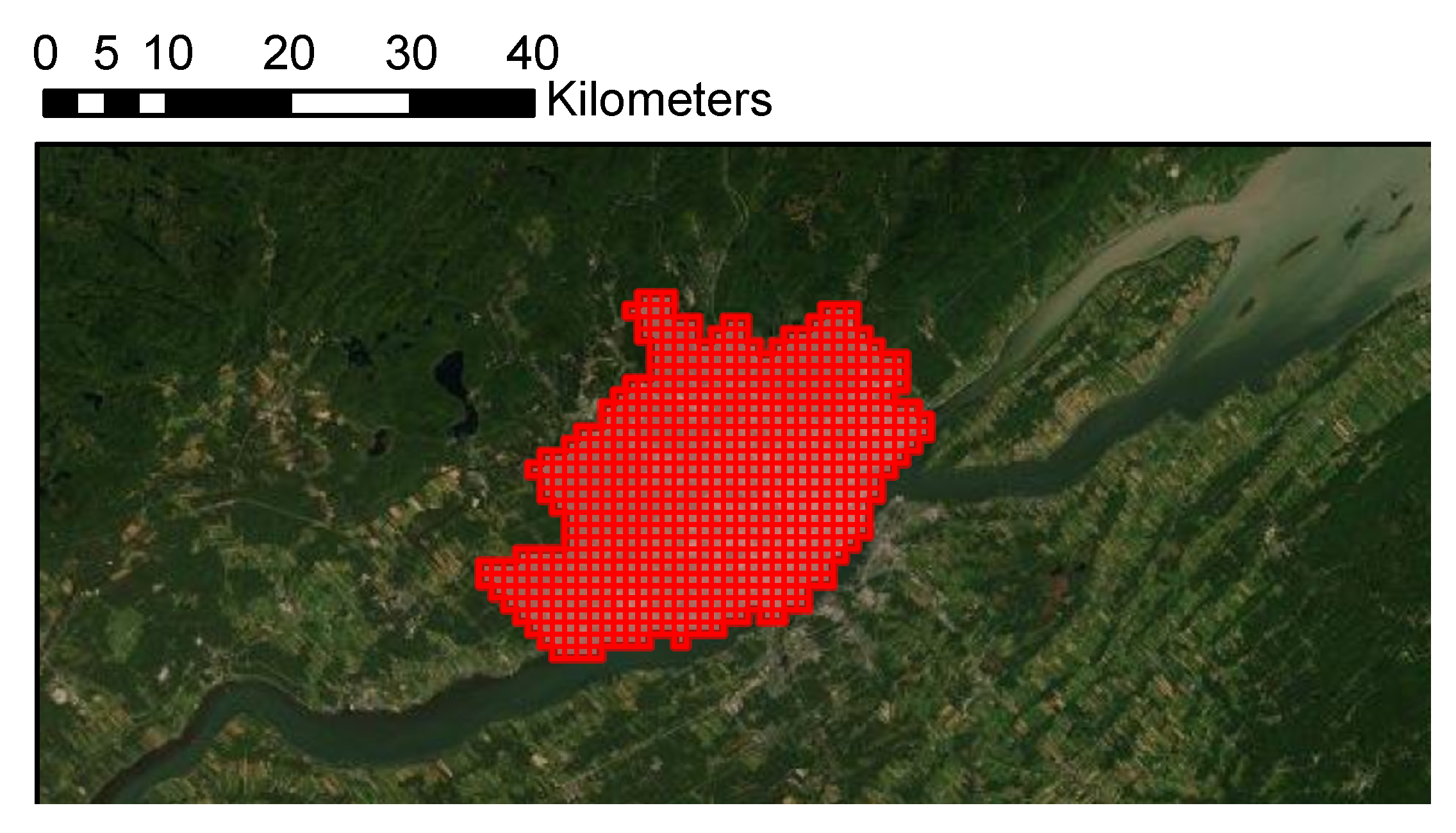
3.2.2. Quebec City Dataset

Besides the assessments on the Vaihingen dataset representing a European urban context, we additionally conduct a performance assessment in another geographic context, namely North America. In this regard, the method is carried out on the urban areas of Quebec City, QC, Canada. They cover a total area of 656 square kilometers. The whole area is divided into tiles of 1 km × 1 km, as shown in Figure 7, for the sake of processing time and memory constraints. The involved LiDAR and optical imagery datasets are described in column four and five of Table 1. The ground truth boundaries of buildings in the whole test area are provided and updated monthly by the City of Quebec, named Empreintes des bâtiments [56]. The ground truth dataset used in this work was downloaded on 4 March 2019.
In March 2019, Microsoft released an open Canada building footprint dataset (consisting of twelve million buildings) collaborating with Statistics Canada [57]. The dataset covers all the Quebec City territory with more than two hundred thousand building footprints. This work is carried out using a deep neural network, of which the foundation is the ResNet-34 [58]. The training set consists of three million labeled Bing images. In this paper, we conduct an individual performance assessment using the mentioned ground truth building boundaries in Quebec City, in order to compare with the SRSM results.
It should be noted that this assessment does not only allow evaluating the performance of the proposed SRSM on such a large dataset, but it also serves as an example demonstrating the scale of the study—i.e., the Quebec province, in which other cities and large areas should not cause any adaptability problem on such an unsupervised method.

3.3. Performance Evaluation of the Super-Resolution

Besides the visual assessment provided in Section 2.2.1, the performance of the proposed SR process is also quantitatively evaluated. We compare it with other conventional 2-D interpolation methods, namely nearest neighbor (NN), bilinear, and natural interpolation [59]. This evaluation and comparison are depicted by Figure 8. The four methods are examined on a real LiDAR point cloud with an average density of 3.8 points/m2 (Figure 8a). Such point cloud is then subsampled by a chosen factor, namely 2, 4, and 8, yielding a subsampled point cloud which serves as an input for these SR/interpolation methods. These experimented factors are chosen based on the proportion between the respective spatial resolution of the datasets (cf. Table 1). For example, Figure 8b depicts the 3-D point cloud subsampled by a factor of 2. Based on the sparse DSM generated from this subsampled point cloud (Figure 8c), each interpolation method generates a DSM having the spatial resolution equal to that of the subsampled LiDAR point cloud times the upscaling factor—in other words, equivalent to the spatial resolution of the original point cloud. The resulting interpolated DSM provided by each method (e.g., Figure 8d,e) is compared with the DSM generated from the full-resolution LiDAR point cloud, which is considered as the ground truth for the assessment (Figure 8f).
In order to evaluate the quality of these interpolation and SR methods—i.e., the closeness between the interpolated image and the ground truth image—we measure the following metrics: root-mean-square error (RMSE), structural similarity (SSIM) [60], and the peak signal-to-noise ratio (PSNR). SSIM and PSNR are two widely used objective metrics for evaluating image super-resolution quality [61]. Their mathematical explanations can be found in Appendix B. Table 2 summarizes the quality measurements of each interpolation method for all three upscaling factors, i.e., × 2 , × 4 and × 8 .
Overall, compared to the other methods, the proposed SR process yields better results, i.e., smaller RMSE, higher SSIM and PSNR. However, it yields a disadvantageous SSIM compared to the natural interpolation and the bilinear interpolation, in the × 4 and × 8 upscaling. Considering the RMSE, one can remark that the improvement in the case of × 2 upscaling between the proposed SR and the others is only marginal (i.e., 1.96 compared to 2.00–2.18). In contrast, in the × 4 and × 8 upscaling, this margin of RMSE improvement becomes more significant. Similar remarks can be made when considering the PSNR. These improved quality measures show that the proposed SR is more reliable compared to the conventional interpolation methods. This quantitative assessment and the visual assessment (previously presented in Section 2.2.1) have demonstrated the relevance of the proposed SR method. It is deemed to fit the purpose to be used in the proposed SRSM.

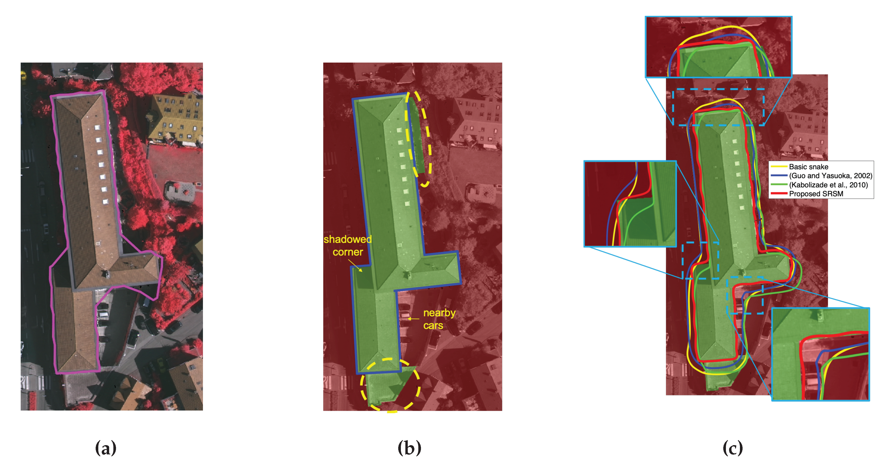
3.4. Comparison between Snake Models

We also perform an assessment on the performance of the proposed SRSM and compare it with other existing snake models previously mentioned in Section 1.3. They are carried out on the gable-roof building previously discussed in Section 2.2 and displayed in Figure 5. First, the ground truth building region is overlaid by a transparent green area, while the surrounding ground is displayed in transparent red color, as in Figure 9b. These overlaying colors allow assessing the building extraction more straightforwardly. Figure 9c presents the result of snake models on the exemplified building. Four snake models are compared, namely basic snake with GVF, snake model of Guo and Yasuoka [33], snake model of Kabolizade et al. [35], and the proposed SRSM. They all are unsupervised snake models, which are substantially different from each other. In addition, they are not constrained to one particular range of building sizes. These also are the reasons why the snake model-based methods [36,37,42] are not involved in this comparison. The snake parameters are set as follows, α = β = 0.2 , balloon force magnitude κ = 0.1 , and image-based energy term weights w l i n e = 0.04 , w e d g e = 2 , w t e r m = 0.01 .
Here, all concerned snake models are initialized by the same LiDAR-based building boundary. These initial points are already an improvement compared to the ones proposed in the respective snake model. However, one can remark in Figure 9c that the other snake models (i.e., the basic snake, the snake model of Guo and Yasuoka [33], and the snake model of Kabolizade et al. [35]) have problems approaching the true edges of the building. On the other hand, the proposed SRSM, under the influence of salient features of the z-image, converges very well towards the edges and the corners. As we previously stated in Section 2.2, this exemplified building involves many challenging regions. One of them is the building corner under shadow (circled in green in Figure 5e), which is now shown in the left subfigure in Figure 9c. Another difficult region is found with many nearby cars (circled in red in Figure 5e). It is now zoomed in the bottom-right subfigure in Figure 9c. It is shown that, on these two corner regions, all three of the previous snake models yield poor results. In contrast, the proposed SRSM approaches very well the ground truth boundary. This visual assessment shows that the z-image-based snake model yields much more accurate building boundary compared to other existing snake models.
Table 3 summarizes the quantitative results of the compared snake models, based on the area-based Quality and RMSE metrics. First of all, one can remark that, in general, the resulting Quality and RSME from all snake models are relatively high (more than 70%). This stems from the benefit of using the LiDAR-based building boundary as initial points. Then, the quantitative results also show the relevance of the proposed snake models, compared to other snake models. However, the margin of gain between them according to these values—i.e., a maximum Quality gain of 9.33% between the basic and the SRSM—is not as high as expected, given the clear advantage drawn from the visual assessment from Figure 9c.
One can also remark that the snake models were not able to extract two particular parts of the building (highlighted by yellow-dashed circles in Figure 9b) because they do not exhibit significant elevation change or color change from the surrounding ground (cf. Figure 5). On one hand, the inability of the SRSM stems from the absence of elevation changes. On the other hand, the other snake models are unable to extract these parts because of the absence of color changes. We are convinced that these undetected parts can be the reason for the low margin between the snake models mentioned above. Therefore, we also conduct another evaluation of all four snake models with a modified version of the ground truth building boundary, in which the two undetected parts are removed. Such a modified ground truth boundary aims to provide the unbiased reference for the snake models. In Figure 9b, this modified ground truth boundary is depicted in blue outlines. The columns 4 and 5 of Table 3 reveal the involved comparison based on this modified ground truth. As expected, the new margin between the proposed snake model and the others is now much larger, i.e., a margin of 21.21% of Quality between the basic snake model and the proposed SRSM. It is coherent with the inference drawn from the visual assessment (Figure 9c). This comparison has shown that the proposed SRSM yields better accuracy than the other snake models. In the next two subsections, the overall performance of the SRSM on different datasets will be assessed.

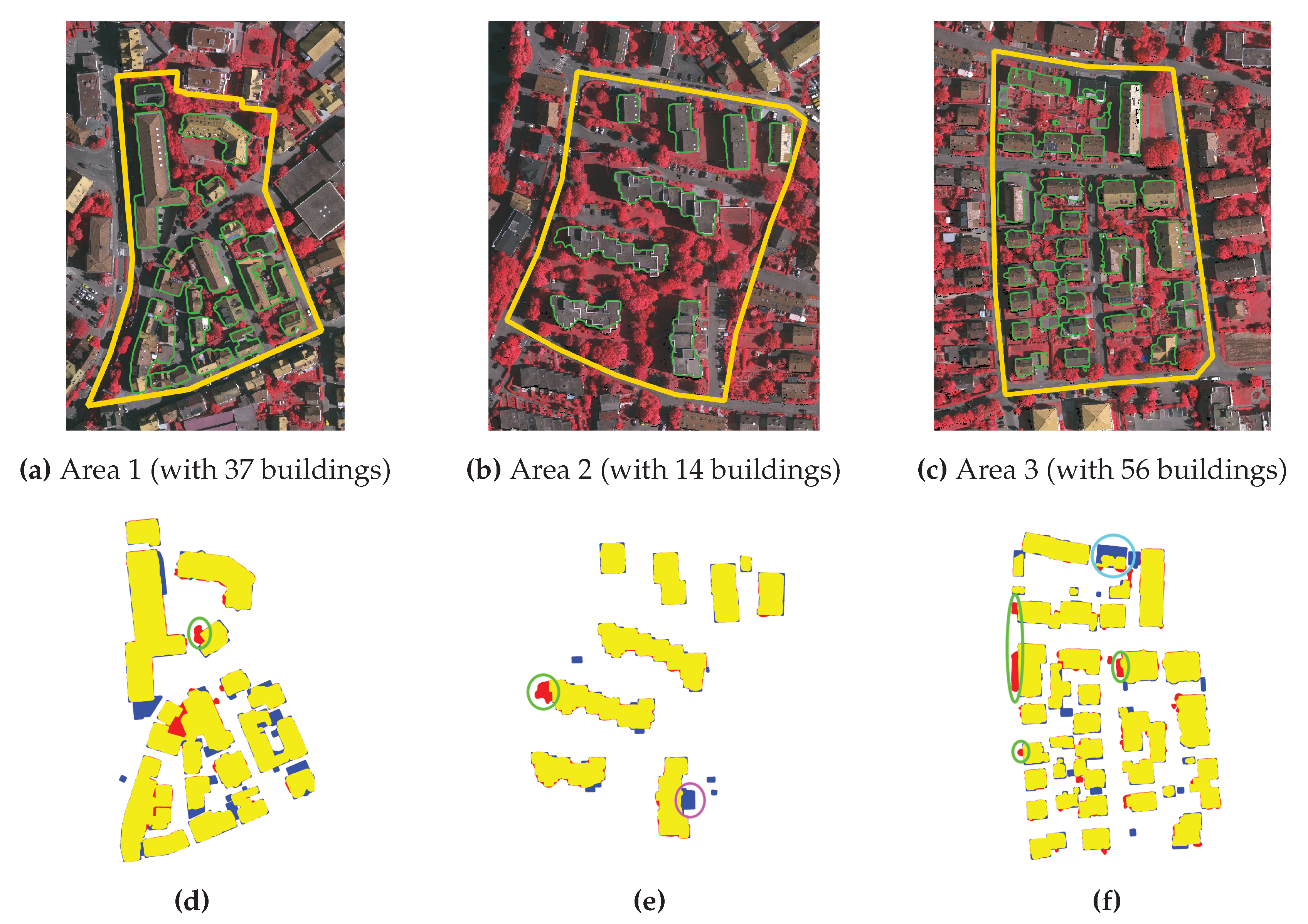
3.5. Performance on ISPRS Vaihingen Dataset

The three test areas of the ISPRS Vaihingen dataset are shown by Figure 10. Area 1 (Figure 10a) is situated in the center of the city and characterized by dense construction consisting of historic buildings with rather complex shapes. Area 2 (Figure 10b) is composed of high-rise residential buildings surrounded by trees. Lastly, Area 3 (Figure 10c) is residential with detached houses and many surrounding trees. The results of SRSM are also depicted in Figure 10a–c in green. Then, Figure 10d–f illustrate the area-based accuracy assessment, denoting TP (in yellow), FP (in red), and FN (in blue) pixels. Overall, the proposed method yields a very high accuracy, reflected by a very high number of TPs on all three areas. However, a number of unresolved problems can be remarked in Figure 10. Firstly, many FP pixels can still be noted in all three areas. They relate to the problem of shadowed tree regions near buildings. Such tree regions are circled in green in Figure 10d–f. An example of this problem is from Area 2, which is shown by Figure 10a. Secondly, several small buildings from all three areas have not been detected.
Table 4 summarizes the area-based accuracy assessment result on all three test areas. In averaging on three areas, the proposed SRSM achieves a Quality of 86.57%, a Completeness of 91.63%, and a Correctness of 93.99%. The last column of Table 4 shows the resulting geometrical accuracy of the SRSM. It can be noted that the RMSE on Area 3 is much lower than the other areas. This is due to the fact that Area 3 is composed of mostly rectangular buildings and it is less complex than the other areas.
Table 5 presents the resulting object-based accuracy of the SRSM. Columns two to four show the accuracy metrics on all objects, whereas columns five to seven provide the metrics when considering only objects with an area larger than 50 m2. The differences between these two results reflect the aforementioned problem of undetected small buildings.
In addition, several buildings have only been partially extracted, due to the fact that the non-extracted parts have very similar elevation to their surrounding area. Particularly, one of these building parts (circled in magenta in Figure 10e), in reality, is the roof of a basement covered by vegetation in Area 2, as shown in Figure 11b. This part has not been extracted by any existing building extraction methods submitted to this benchmark [26]. In Area 3, there is also one building (circled in cyan in Figure 10f) that is very poorly extracted. This problem is caused by the incompleteness of LiDAR data on this building, as shown in Figure 11c.
The resulting accuracy of the SRSM is then compared with other works submitted to the ISPRS Vaihingen benchmark portal [62]. As of 26 January 2020, there were 42 submitted methods. Four histograms are shown by Figure 12, summarizing the resulting accuracy of these methods averaged on the three areas. Each histogram shows the distribution of methods according to the area-based Quality (Figure 12a), object-based Quality (Figure 12b), object-based Quality for objects larger than 50 m2 (Figure 12c), and RMSE (Figure 12d). All four histograms are presented with their bins sorted in an increasing quality order, i.e., any particular bin involves a higher quality (i.e., higher Quality percentage and lower RMSE) than the bins on its left. Through these histograms, one can remark on the developed consensus on results of the state-of-the-art methods. For instance, from Figure 12a, it is shown that the majority of the methods (i.e., approximately 62% or 26/42 methods) yield an area-based Quality ranging from 82.5% to 89.8%. On the other hand, 64% of the methods yield an object-based Quality ranging from 73.8% to 87.2% (Figure 12b). For object-based Quality for buildings larger than 50 m2 (Figure 12c), a result greater than 97.6% is desirable, considering that 62% of the methods are capable of yielding such an outcome.
As a fully unsupervised and automatic building extraction method, our method yields very high accuracy. Indeed, considering the resulting average area-based and object-based Quality, respectively 86.57% and 81.60%, our method is placed among the top 20% of all benchmark methods, i.e., the 10th or 9th among 42 methods. These results are highly desirable compared to other existing methods. It is also worth noting that many among the top-accuracy methods are supervised or model-based methods [26]. Indeed, the supervised methods proposed by Niemeyer et al. [27] and Chai [28] result in area-based Quality of, respectively, 87.8% and 89.7%. The model-based methods proposed by Bayer et al. [29] yield an area-based Quality of 89.8%, and the two versions of a method by Grigillo and Kanjir [30] yield an area-based Quality of 89.4% and 89.7%. In addition, considering the object-based Quality for buildings with an area larger than 50 m2, our method is placed 12th among 42 methods. However, considering the RMSE (Figure 12d), our method yields a result (averaging 1.09 m) among the highest RMSE, in other words, the least desirable. Future works will concentrate on improving such accuracy.
The proposed SRSM also faces several problems when performed on the ISPRS Vaihingen benchmark dataset, such as the problem of nearby shadowed vegetation shown in Figure 11a. Grigillo and Kanjir [30] proposed to solve such a problem with the rule-set classifiers on image pixel colors and NDVI. However, this approach involves multiple manually selected thresholds which require a high level of supervision. There also exists other classification approaches (in order to better classify shadowed trees from buildings) involving graph-cut-based method [63]. However, such method may require a high amount of a priori information or user inputs in order to yield accurate results [32]. Therefore, by opting for such mentioned approaches, the level of supervision of the building extraction method should be reconsidered.

3.6. Performance on Quebec City

In order to test the performance and applicability of the proposed SRSM on a large scale, we carry it out on the Quebec City dataset. Many areas in Quebec City are composed of different types of urban, residential, and industrial scenes. Two of these typical scenes are shown in Figure 13. They are also representative of the North American context. Based on a visual assessment, the SRSM succeeds at delineating the building boundaries accurately on the two exemplified scenes. Typically, the size of the buildings shown in both scenes varies greatly from small to very large buildings. One can remark that many buildings that have similar color as their background (i.e., parking lots, open areas, etc.) are also well delineated. Other optical image-related problems such as roof objects and nearby cars are also avoided. This re-emphasizes the benefits of using the z-images encoding LiDAR elevation data instead of the optical images. In addition, similar to the Vaihingen datasets (particularly Area 1 and 2), the shape of buildings presented in these two examples—also verified across the whole Quebec City area—can be very complex. These three factors related to the scene complexity—i.e., varying building size, color, and shape—can be problematic to other methods, whereas the proposed SRSM is able to overcome such complexity.
Table 6 summarizes the area-based and object-based accuracy yielded by the Microsoft open Canada building footprints and the proposed SRSM. It can be noted that the Completeness and Correctness yielded by the two methods are quite different. These differences mainly stem from the fact that the two methods were carried out using different data sources with different characteristics. However, based on the resulting Quality values reflecting the overall accuracy, it can be noted that the SRSM provides a competitive outcome compared to the Microsoft method. Indeed, the Quality margins between the SRSM and the Microsoft method are well balanced. The SRSM yields a 6.65% higher object-based Quality, while in contrast, the Microsoft method provides a 7.40% higher area-based Quality. On the one hand, the difference of the area-based Quality stems from the fact that the resulting footprints from SRSM have the tendency to be slightly “rounded” around the building corners. Whereas the Microsoft footprints were generated (with their own polygonization method) without such a problem. On the other hand, the SRSM with the advantage of the z-images encoding elevation data allows one to detect the buildings more precisely, hence yielding the higher object-based Quality. Nevertheless, it is always worth noting that such competitive accuracy is produced by an unsupervised approach, compared to the heavily supervised approach from Microsoft which was trained on three million labeled images. The complete dataset of extracted building boundaries in Quebec City by the SRSM as well as the high-resolution version of Figure 13, are made publicly available at https://github.com/nthuy190991/SRSM_QuebecCity_building_extraction.
The outcomes of the SRSM on the Quebec City dataset are relevant, visually and quantitatively. However, there still remain two issues. Firstly, from a practical perspective, the SRSM was carried out separately on tiles (Figure 7) for the sake of processing time and memory constraint. Then, the tile-based results were combined in QGIS. Such a step is crucial for the buildings located in the transitioning areas between two neighboring tiles. Several of those buildings can be identified near the borders of the tiles shown in Figure 13. Secondly, the SRSM is unable to separate connected or nearby buildings with similar height. Given the z-images involves only elevation information, such a separation task can be difficult. Therefore, we shall investigate the usefulness of other information for such a task. Overall, these two issues can affect unfavorably the resulting accuracy of the SRSM. Future efforts will concentrate on addressing these two issues to improve the SRSM results.

4. Discussions

In this section, three discussions are addressed: (i) on the relevance of the proposed SR, (ii) on the SRSM results, and (iii) on the impact of the snake model parametrization.

4.1. Relevance of the Super-Resolution

As suggested by the name of the proposed method (i.e., SRSM), the SR process plays a critical role. However, such a process is not only relevant for snake models. Indeed, the need and potential of such a process to enhance the spatial resolution of LiDAR data is high. For instance, in the topic of building extraction, several methods [16,38] proposed to replace the blue channel of RGB images with a normalized DSM (nDSM). Such a composite image—i.e., red, green, and nDSM—is then fed into deep neural networks for extracting buildings. However, these approaches did not account for the fact that the two input images—the RGB image and the nDSM—usually have different resolutions, hence an SR was not proposed. On the other hand, the SR process could resolve one of the problems of the snake model proposed by Kabolizade et al. [35] (cf. Section 1.3). A super-resolved DSM could improve the height variance-based external energy term proposed in their work. However, it is worth-noting that the main drawback of their snake model is still the use of optical image as the target image, i.e., for computing the E img . In other topics, the study of SR applied to LiDAR depth measurements is also very active. Indeed, a reliable SR would benefit many applications, such as calibration for autonomous driving [52] or land cover classification [64].

4.2. Discussion on the SRSM Resulting Footprints

The accuracy level of the SRSM results carried out on the Vaihingen dataset and the Quebec City dataset have been shown—through multiple assessments and comparisons—to be desirable. It has achieved our objectives for a large-scale high-accuracy building extraction method, without any assumptions on the building characteristics nor any training data. However, two important aspects concerning the building footprints provided by the proposed method should be discussed. First, it can be noted from the results in Vaihingen (Figure 10) and Quebec City (Figure 13) that the resulting snakes have the tendency to be slightly “rounded” around building corners. Such a problem can be addressed with an efficient polygonization method. However, such a step can be quite challenging considering the complexity of building shape on the two study areas.
The second aspect worth mentioning involves the acquisition time difference between the LiDAR data, the optical image data, and the reference ground truth boundaries. On the one hand, considering a benchmark dataset like the ISPRS Vaihingen dataset, such an aspect is minimal since the data were acquired almost concurrently (cf. Table 1). In addition, the Vaihingen ground truth building boundaries were prepared using the same data. On the other hand, considering the large scale of Quebec City, such a temporal aspect is much more complicated. Firstly, the LiDAR data were acquired one year after the optical images. Secondly, the Empreintes des bâtiments dataset consisting of the ground truth building boundaries was produced using multiple different sources and updated monthly. Thirdly, the comparative Microsoft results were carried out using Bing Imagery data. Since Bing Imagery is a composite of multiple sources, we are unable to determine the exact dates for individual pieces of data [57]. Such temporal difference and uncertainty can affect the building extraction accuracy. This issue requires a dedicated study in order to account for all of the involved factors.

4.3. Impacts of Snake Parametrization

A snake model involves a number of parameters, such as α , β , κ (the balloon force magnitude), μ GVF (the GVF smoothing parameter), etc. In the existing models [34,35,36], these parameters have been set empirically in order to extract buildings effectively. The snake parametrization becomes extremely difficult over a large extended area. However, some parameters are more important than others. In this regard, Marcos et al. [42] partially addressed such a problem with a CNN-based approach. It involves learning the characteristics of the most important elements of the snake model, namely the snake internal energy term weights ( α and β ), the image-based energy term ( E img ), and the balloon force ( F balloon ). Additionally, they asserted that one scalar value of β for all parts of a building can lead to problems of oversmoothing at building corners and undersmoothing at other regions. To avoid such a problem, they proposed a local penalization approach, by assigning a different β penalization to each pixel depending on whether the pixels are near the building edges or corners, whereas α remains scalar for every pixel.
In this discussion, let us analyze the relevance of such a parametrization approach and compare it with our fixed parametrization for the SRSM. The characteristics of the CNN-inferred energy terms and parameters differ with respect to the features from the optical image (e.g., building corners, edges, etc.), as summarized by Table 7.
Firstly, concerning the balloon force, the second column of Table 7 shows the characteristics of the balloon force inferred by the CNN. If a snake is initialized inside a building boundary, the balloon force—being positive—will inflate it outward until it reaches the building corners and edges. Then, the balloon force sharply drops to zero and remains zero right outside the building boundary, which means that the snake is not allowed to inflate anymore. However, if the snake is provided with initial points outside the building boundary, the balloon force—being null-valued—is unable to shrink inward to approach the building true boundaries. Such behavior is not optimal. In contrast, the approach to generate F balloon proposed in this paper based on the LiDAR-based building mask is more relevant. It allows the snake to be shrunk or inflated adaptively, regardless of where it is initialized, without relying on any learning process.
Secondly, we address the image-based energy term E img . The characteristics of the CNN-inferred image-based energy term E img are revealed in Table 7. However, they are similar to those exhibited by the traditional snake model mathematical approach (cf. Equation (2)). Such a similarity is illustrated by Figure 14. The energy term E img of a rectangular building (Figure 14a) is mathematically computed and shown in Figure 14b. As illustrated, the building edges and corners exhibit negative to very negative values, whereas the pixels inside and outside of the building exhibit positive values. Such characteristics among building features are analogous to the CNN-based approach. Therefore, in the proposed SRSM, the energy term E img is retained as in the traditional snake model. The sole change is that the target image is the z-image instead of the optical image. Such a change is relevant as the z-image-based energy term provides more desirable features—i.e., height changes instead of color changes.
Lastly, concerning the snake curvature weight β , we retain the use of a fixed scalar β in our method. The immediate reason is that without a training phase, the generation of a different β value for each pixel is difficult, or even virtually impossible. In addition, as we changed the target image of the snake model, the needed dynamics for β should also change. Since the only sources of attraction for the snake model are now the height changes from off-terrain objects, the snake curvature does not need to be different pixel to pixel. The snake should be able to correct itself from such sources of attraction. A comparison is conducted to confirm whether using the CNN-inferred pixel-wise β would bring a real benefit compared with a fixed scalar β . As such, the SRSM is experimented with where the value of α and β are, either inferred from CNN as in [42] or set to fixed scalar values. Such a comparison is carried out on seven buildings in the proximity of Area 1 (ISPRS benchmark dataset) selected by Marcos et al. [42]. One of these buildings is exemplified in Figure 15. The optical image and the initial points for SRSM in blue are revealed in Figure 15a, whereas the z-image is shown in Figure 15b. These initial points were used in the work of Marcos et al. [42] and also in this comparison. The SRSM carried out with the CNN-inferred α and β results in the building boundary in green (Figure 15a). The CNN-inferred value of α is 0.767, whereas the image of β values (each pixel with a different β value) is shown by Figure 15c. Then, the SRSM carried out using the scalar α and β —both set equal to 0.2—yields the red building boundary (Figure 15a). The two snakes in red and in green are shown to be similar. Quantitatively, the area-based Quality provided by the CNN-based approach on all seven buildings averages 73.62%, whereas the fixed scalar parametrization approach yields 72.03%. By visual and quantitative assessment, it is shown that the CNN-inferred approach as well as the pixel-wise β does not bring a practical benefit to our SRSM.
In summary, the proposed SRSM succeeds in providing a relevant solution, regarding all three main aspects of the snake parameterization. Indeed, since almost every building exhibits a strong elevation variation with respect to its surrounding area, the characteristics of building appearances on their respective z-image should all be similar. As a result, the proposed SRSM can be generalized with the same set of influential parameters on buildings of various size and shape as well as in complex environments.

5. Conclusions

In this paper, we proposed and evaluated an unsupervised and automatic building extraction method dedicated to a large-scale urban scene. This method is built around an efficient snake model, named SRSM. First, a preliminary extraction of building boundaries from the LiDAR point cloud is carried out. These boundaries are used as initial points for the SRSM as well as in the improved balloon force. Second, in order to resolve the sparsity problem related to the LiDAR data spatial resolution compared to an optical imagery dataset [21], we propose a super-resolution process. Such a process is devoted to the projection and propagation of LiDAR data onto the image space, enabling the augmentation of its spatial resolution. Then, the snake model is carried out based on the resulting z-images. Such z-images encoding LiDAR elevation data are highly beneficial since the height changes provide a more reliable cue for extracting buildings than the spectral and textural changes provided by the optical images. In addition to such a benefit, the useful elevation data are now provided with high spatial resolution. Third, the balloon force is improved to behave more adaptively compared to the classical balloon force.
By using the z-image, a number of typical problems related to the optical image have also been addressed. Until now, all of the existing snake models have conceded the sensitivity problem against image noises and details, such as roof objects and nearby cars and trees. Such scene elements prompt undesired sources of attraction, causing the snake model to be unable to converge toward the true building edges. Operating on the z-image which only exhibits significant height changes, the SRSM is provided with relevant sources of attraction. In addition, such a fundamental replacement—i.e., using, the z-image instead of the optical image—also affects the parametrization of the snake model. Indeed, the need for a hyperparameter tuning, e.g., by a deep learning approach [42], becomes less substantial. Thus, the SRSM is parametrized with fixed scalar values. By the virtue of the proposed improvements, such static parametrization does not restrain the applicability and scalability of the z-image-based snake model over large extended area. A comprehensive comparison and discussion of this parametrization with the deep learning approach by [42] has also been carried out in this paper.
Concerning the performance assessment, the SRSM is tested in two different geographical contexts, namely Europe (with the Vaihingen benchmark dataset) and North America (with the Quebec City dataset). The two contexts involve various differences in terms of compactness, density, and regularity of urban areas [43]. The proposed SRSM yields very high accuracy on the ISPRS Vaihingen benchmark dataset, namely 86.57% of area-based Quality and 81.60% of object-based Quality. These values show that the SRSM is highly desirable, especially as a fully unsupervised method, as opposed to many other high-accuracy methods. Concerning the Quebec City dataset with the total area of 656 km2, the SRSM succeeds at providing a relatively high accuracy, namely area-based Quality of 62.37% and object-based Quality of 63.21%. Such an accuracy level on this dataset may seem less desirable than the one on the Vaihingen dataset mentioned above. However, it can be well expected on such a large-scale dataset, with various types of complex residential, urban, and industrial scenes. Indeed, compared to the building footprints produced by Microsoft by a deep neural network approach, our unsupervised method succeeds at providing a competitive accuracy level. The two geographical contexts also show the very high capacity of the SRSM for extending over very large and complex areas. With the proposed SRSM, this study has achieved our objectives for a scalable, versatile, and accurate building extraction solution. Indeed, in the context of the flood risk assessment in the province of Quebec, such a method—capable of yielding accurate building footprint boundaries and locations in such a large scale—enables us to achieve subsequent critical tasks, namely the extraction of building structural and occupational characteristics. Future works will focus on improving the resulting geometrical accuracy, as well as on several remaining problems such as shadowed vegetation and misdetection of small buildings.

Author Contributions

Conceptualization, T.H.N.; Funding acquisition, S.D., D.G., C.S., and J.-M.L.C.; Investigation, T.H.N., S.D.; Methodology, T.H.N.; Project administration, S.D.; Resources, S.D., D.G., C.S., and J.-M.L.C.; Supervision, S.D., J.-M.L.C.; Validation, T.H.N., S.D.; Visualization, T.H.N.; Writing—original draft preparation, T.H.N.; Writing—review and editing, T.H.N., S.D., D.G., C.S., and J.-M.L.C. All authors have read and agreed to the published version of the manuscript.

Funding

This research was funded in part by the Ministère de la Sécurité publique, Gouvernement du Québec, Canada, project ORACLE-2, in part by the Natural Sciences and Engineering Research Council of Canada (NSERC) grant number RGPIN-2018-04046, and in part by the Brittany region, France.

Acknowledgments

The authors would like to thank the Centre GéoStat (Université Laval), as well as the Communauté Métropolitaine de Québec (QC, Canada) for providing the Quebec City datasets used in this work. They also would like to thank the City of Quebec for providing the Empreintes des bâtiments dataset used as ground truth building footprints in this work. A special thanks goes to Eric Janssens-Coron from the Centre de Recherche en Données et Intelligence Géospatiales (Université Laval) for his help on the management of the Quebec City datasets. They also would like to thank the Microsoft Bing Maps team for developing and releasing the open Canada building footprints. The Vaihingen dataset was provided by the German Society for Photogrammetry, Remote Sensing and Geoinformation (DGPF) [55]. Lastly, they would like to thank Dirk-Jan Kroon from University of Twente for his contributions to the development of the conventional snake models.

Conflicts of Interest

The authors declare no conflict of interest.

Abbreviations

The following abbreviations are used in this manuscript:
CNNConvolutional Neural Network
DSMDigital Surface Model
DTMDigital Terrain Model
FCNFully Convolutional Neural Network
FISTAFast Iterative Shrinkage-Thresholding Algorithm
GVFGradient Vector Flow
ISTAIterative Shrinkage-Thresholding Algorithm
LiDARLight Detection And Ranging
NDVINormalized Difference Vegetation Index
RMSERoot Mean Square Error
SSDGSum of squared directional gradients
SRSuper-resolution
SRSMSuper-resolution-based Snake Model

Appendix A. External Image-Based Energy Term of Snake Model

The line functional is defined based on the intensity of the image I ( x , y ) , with a filter for smoothing or noise reduction, such as Gaussian filter:
E l i n e = G σ ( x , y ) I ( x , y )
The edge functional is based on the image gradient, which attracts the snake to move towards the edges with high gradient value.
E e d g e = G σ ( x , y ) I ( x , y ) 2
where G σ ( x , y ) is a two-dimensional Gaussian function with a standard deviation σ and * denotes the 2-D convolution operator.
Curvature of level lines in a slightly smoothed image can be used to detect corners and line segment terminations in an image. Using this method, let C ( x , y ) = G σ I ( x , y ) be the smoothed image. With an angle θ = tan 1 ( C y / C x ) , the unit vectors which are along and perpendicular to the gradient direction are:
n = ( cos θ , sin θ ) , n = ( sin θ , cos θ )
The termination functional of energy is defined as:
E t e r m = θ n = 2 C / n 2 C / n = C y y C x 2 2 C x y C x C y + C x x C y 2 ( C x 2 + C y 2 ) 3 / 2

Appendix B. Super-Solution Quality Metrics

Given the super-resolved image I and the reference image R, the Structural Similarity (SSIM) quality assessment index is based on the computation of three terms, namely the luminance term, the contrast term, and the structural term.
SSIM ( I , R ) = l ( I , R ) γ · c ( I , R ) δ · s ( I , R ) ϵ
where
l ( X , Y ) = 2 μ X μ Y + C 1 μ X 2 + μ Y 2 + C 1 , c ( X , Y ) = 2 σ X σ Y + C 2 σ X 2 + σ Y 2 + C 2 , s ( X , Y ) = σ X Y + C 3 σ X σ Y + C 3
with μ X , μ Y , σ X , σ Y , and σ X Y respectively are the local means, standard deviations, and cross-covariance for images X and Y. The parameters for SSIM index are set as follows, γ = δ = ϵ = 1 ; and C 1 = ( 0.01 × L ) 2 , C 2 = ( 0.03 × L ) 2 , C 3 = C 2 / 2 , where L = 2 # bits   per   pixels 1 denotes the dynamic range value of the images. With these parameters, the SSIM index (A5) is simplified into,
SSIM ( I , R ) = 2 μ I μ R + C 1 μ I 2 + μ R 2 + C 1 · 2 σ I , R + C 2 σ I 2 + σ R 2 + C 2
Another metric for evaluating a method of super-resolution of image is Peak Signal-to-Noise Ratio (PSNR) in decibels, which is defined by Equation (A8).
PSNR ( I , R ) = 10 × log 10 peak _ val 2 MSE ( I , R )
where peak _ val is the maximum possible value of the images, and MSE is the mean square error between I and R.

References

  1. Frédéricque, B.; Daniel, S.; Bédard, Y.; Paparoditis, N. Populating a building Multi Representation Data Base with photogrammetric tools: Recent progress. ISPRS J. Photogramm. Remote Sens. 2008, 63, 441–460. [Google Scholar] [CrossRef]
  2. Daniel, S.; Doran, M.A. GeoSmartCity: Geomatics Contribution to the Smart City. In Proceedings of the 14th Annual International Conference on Digital Government Research, Quebec, QC, Canada, 17–20 June 2013; pp. 65–71. [Google Scholar]
  3. Xie, Y.; Weng, A.; Weng, Q. Population estimation of urban residential communities using remotely sensed morphologic data. IEEE Geosci. Remote Sens. Lett. 2015, 12, 1111–1115. [Google Scholar]
  4. Al-Khudhairy, D.H. Geo-spatial information and technologies in support of EU crisis management. Int. J. Digit. Earth 2010, 3, 16–30. [Google Scholar] [CrossRef]
  5. Alamdar, F.; Kalantari, M.; Rajabifard, A. Towards multi-agency sensor information integration for disaster management. Comput. Environ. Urban Syst. 2016, 56, 68–85. [Google Scholar] [CrossRef]
  6. Blin, P.; Leclerc, M.; Secretan, Y.; Morse, B. Cartographie du risque unitaire d’endommagement (CRUE) par inondations pour les résidences unifamiliales du Québec. Rev. Sci. EAU 2005, 18, 427–451. [Google Scholar] [CrossRef] [Green Version]
  7. El-Rewini, H.; Abd-El-Barr, M. Advanced Computer Architecture and Parallel Processing; John Wiley & Sons: Hoboken, NJ, USA, 2005; Volume 42. [Google Scholar]
  8. Kim, T.; Muller, J.P. Development of a graph-based approach for building detection. Image Vision Comput. 1999, 17, 3–14. [Google Scholar] [CrossRef]
  9. Karantzalos, K.; Paragios, N. Recognition-driven two-dimensional competing priors toward automatic and accurate building detection. IEEE Trans. Geosci. Remote Sens. 2008, 47, 133–144. [Google Scholar] [CrossRef]
  10. Ngo, T.T.; Mazet, V.; Collet, C.; De Fraipont, P. Shape-based building detection in visible band images using shadow information. IEEE J. Sel. Top. Appl. Earth Obs. Remote Sens. 2016, 10, 920–932. [Google Scholar] [CrossRef]
  11. Gruen, A.; Wang, X. News from CyberCity-Modeler. In Proceedings of the 3rd International Workshop on Automatic Extraction of Man-Made Objects from Aerial and Space Images. Monte Verita, Ascona, Switzerland, 10–15 June 2001; pp. 93–101. [Google Scholar]
  12. Tomljenovic, I.; Höfle, B.; Tiede, D.; Blaschke, T. Building extraction from airborne laser scanning data: An analysis of the state of the art. Remote Sens. 2015, 7, 3826–3862. [Google Scholar] [CrossRef] [Green Version]
  13. Huertas, A.; Nevatia, R. Detecting buildings in aerial images. Comput. Vis. Graph. Image Process. (CVGIP) 1988, 41, 131–152. [Google Scholar] [CrossRef]
  14. Lee, D.S.; Shan, J.; Bethel, J.S. Class-guided building extraction from Ikonos imagery. Photogramm. Eng. Remote Sens. 2003, 69, 143–150. [Google Scholar] [CrossRef] [Green Version]
  15. Turker, M.; Koc-San, D. Building extraction from high-resolution optical spaceborne images using the integration of support vector machine (SVM) classification, Hough transformation and perceptual grouping. Int. J. Appl. Earth Obs. Geoinf. 2015, 34, 58–69. [Google Scholar] [CrossRef]
  16. Huang, J.; Zhang, X.; Xin, Q.; Sun, Y.; Zhang, P. Automatic building extraction from high-resolution aerial images and LiDAR data using gated residual refinement network. ISPRS J. Photogramm. Remote Sens. 2019, 151, 91–105. [Google Scholar] [CrossRef]
  17. Ekhtari, N.; Zoej, M.J.V.; Sahebi, M.R.; Mohammadzadeh, A. Automatic building extraction from LIDAR digital elevation models and WorldView imagery. J. Appl. Remote Sens. 2009, 3, 033571. [Google Scholar] [CrossRef]
  18. Khoshelham, K.; Elberink, S.O.; Xu, S. Segment-based classification of damaged building roofs in aerial laser scanning data. IEEE Geosci. Remote Sens. Lett. 2013, 10, 1258–1262. [Google Scholar] [CrossRef]
  19. Zhang, J.; Lin, X.; Ning, X. SVM-based classification of segmented airborne LiDAR point clouds in urban areas. Remote Sens. 2013, 5, 3749–3775. [Google Scholar] [CrossRef] [Green Version]
  20. Zhang, J.; Lin, X. Advances in fusion of optical imagery and LiDAR point cloud applied to photogrammetry and remote sensing. Int. J. Image Data Fusion 2017, 8, 1–31. [Google Scholar] [CrossRef]
  21. Chen, L.; Zhao, S.; Han, W.; Li, Y. Building detection in an urban area using lidar data and QuickBird imagery. Int. J. Remote Sens. 2012, 33, 5135–5148. [Google Scholar] [CrossRef]
  22. Sohn, G.; Dowman, I. Data fusion of high-resolution satellite imagery and LiDAR data for automatic building extraction. ISPRS J. Photogramm. Remote Sens. 2007, 62, 43–63. [Google Scholar] [CrossRef]
  23. Awrangjeb, M.; Zhang, C.; Fraser, C.S. Automatic extraction of building roofs using LIDAR data and multispectral imagery. ISPRS J. Photogramm. Remote Sens. 2013, 83, 1–18. [Google Scholar] [CrossRef] [Green Version]
  24. Zhang, J. Multi-source remote sensing data fusion: Status and trends. Int. J. Image Data Fusion 2010, 1, 5–24. [Google Scholar] [CrossRef] [Green Version]
  25. Gilani, S.; Awrangjeb, M.; Lu, G. An automatic building extraction and regularisation technique using lidar point cloud data and orthoimage. Remote Sens. 2016, 8, 258. [Google Scholar] [CrossRef] [Green Version]
  26. Rottensteiner, F.; Sohn, G.; Gerke, M.; Wegner, J.D.; Breitkopf, U.; Jung, J. Results of the ISPRS benchmark on urban object detection and 3D building reconstruction. ISPRS J. Photogramm. Remote Sens. 2014, 93, 256–271. [Google Scholar] [CrossRef]
  27. Niemeyer, J.; Rottensteiner, F.; Soergel, U. Conditional random fields for lidar point cloud classification in complex urban areas. ISPRS Ann. Photogramm. Remote Sens. Spat. Inf. Sci 2012, 1, 263–268. [Google Scholar] [CrossRef] [Green Version]
  28. Chai, D. A probabilistic framework for building extraction from airborne color image and DSM. IEEE J. Sel. Top. Appl. Earth Obs. Remote Sens. 2016, 10, 948–959. [Google Scholar] [CrossRef]
  29. Bayer, S.; Poznanska, A.; Dahlke, D.; Bucher, T. Brief description of Procedures Used for Building and Tree Detection at Vaihingen Test Site. Available online: http://ftp.ipi.uni-hannover.de/ISPRS_WGIII_website/ISPRSIII_4_Test_results/papers/Bayer_etal_DLR_detection_buildings_trees_Vaihingen.pdf (accessed on 26 January 2020).
  30. Grigillo, D.; Kanjir, U. Urban object extraction from digital surface model and digital aerial images. ISPRS Ann. Photogramm. Remote Sens. Spat. Inf. Sci 2012, 3, 215–220. [Google Scholar] [CrossRef] [Green Version]
  31. Kass, M.; Witkin, A.; Terzopoulos, D. Snakes: Active contour models. Int. J. Comput. Vis. 1988, 1, 321–331. [Google Scholar] [CrossRef]
  32. Szeliski, R. Computer Vision: Algorithms and Applications, 1st ed.; Springer: Berlin/Heidelberg, Germany, 2010. [Google Scholar]
  33. Guo, T.; Yasuoka, Y. Snake-based approach for building extraction from high-resolution satellite images and height data in urban areas. In Proceedings of the 23rd Asian conference on remote sensing (ACRS), Kathmandu, Nepal, 25–29 November 2002; p. 6. [Google Scholar]
  34. Peng, J.; Zhang, D.; Liu, Y. An improved snake model for building detection from urban aerial images. Pattern Recognit. Lett. 2005, 26, 587–595. [Google Scholar] [CrossRef]
  35. Kabolizade, M.; Ebadi, H.; Ahmadi, S. An improved snake model for automatic extraction of buildings from urban aerial images and LiDAR data. Comput. Environ. Urban Syst. 2010, 34, 435–441. [Google Scholar] [CrossRef]
  36. Ahmadi, S.; Zoej, M.V.; Ebadi, H.; Moghaddam, H.A.; Mohammadzadeh, A. Automatic urban building boundary extraction from high resolution aerial images using an innovative model of active contours. Int. J. Appl. Earth Obs. Geoinf. 2010, 12, 150–157. [Google Scholar] [CrossRef]
  37. Fazan, A.J.; Dal Poz, A.P. Rectilinear building roof contour extraction based on snakes and dynamic programming. Int. J. Appl. Earth Obs. Geoinf. 2013, 25, 1–10. [Google Scholar] [CrossRef]
  38. Griffiths, D.; Boehm, J. Improving public data for building segmentation from Convolutional Neural Networks (CNNs) for fused airborne lidar and image data using active contours. ISPRS J. Photogramm. Remote Sens. 2019, 154, 70–83. [Google Scholar] [CrossRef]
  39. Nguyen, T.H.; Daniel, S.; Guériot, D.; Sintès, C.; Le Caillec, J.M. Unsupervised Automatic Building Extraction Using Active Contour Model on Unregistered Optical Imagery and Airborne LiDAR Data. ISPRS - Int. Arch. Photogramm. Remote Sens. Spatial Inf. Sci. 2019, XLII-2/W16, 181–188. [Google Scholar] [CrossRef] [Green Version]
  40. Awrangjeb, M.; Lu, G.; Fraser, C. Automatic building extraction from LiDAR data covering complex urban scenes. ISPRS - Int. Arch. Photogramm. Remote Sens. Spatial Inf. Sci. 2014, 40, 25. [Google Scholar] [CrossRef] [Green Version]
  41. Yang, B.; Xu, W.; Dong, Z. Automated extraction of building outlines from airborne laser scanning point clouds. IEEE Geosci. Remote Sens. Lett. 2013, 10, 1399–1403. [Google Scholar] [CrossRef]
  42. Marcos, D.; Tuia, D.; Kellenberger, B.; Zhang, L.; Bai, M.; Liao, R.; Urtasun, R. Learning deep structured active contours end-to-end. In Proceedings of the IEEE Conference on Computer Vision and Pattern Recognition, Salt Lake City, UT, USA, 18–23 June 2018; pp. 8877–8885. [Google Scholar] [CrossRef] [Green Version]
  43. Huang, J.; Lu, X.X.; Sellers, J.M. A global comparative analysis of urban form: Applying spatial metrics and remote sensing. Landsc. Urban Plan. 2007, 82, 184–197. [Google Scholar] [CrossRef]
  44. Zhang, W.; Qi, J.; Wan, P.; Wang, H.; Xie, D.; Wang, X.; Yan, G. An easy-to-use airborne LiDAR data filtering method based on cloth simulation. Remote Sens. 2016, 8, 501. [Google Scholar] [CrossRef]
  45. Awrangjeb, M.; Ravanbakhsh, M.; Fraser, C.S. Automatic detection of residential buildings using LIDAR data and multispectral imagery. ISPRS J. Photogramm. Remote Sens. 2010, 65, 457–467. [Google Scholar] [CrossRef] [Green Version]
  46. Rottensteiner, F.; Trinder, J.; Clode, S.; Kubik, K. Building detection by fusion of airborne laser scanner data and multi-spectral images: Performance evaluation and sensitivity analysis. ISPRS J. Photogramm. Remote Sens. 2007, 62, 135–149. [Google Scholar] [CrossRef]
  47. Nguyen, T.H.; Daniel, S.; Guériot, D.; Sintes, C.; Le Caillec, J.M. Robust Building-Based Registration of Airborne Lidar Data and Optical Imagery on Urban Scenes. In Proceedings of the IGARSS 2019-2019 IEEE International Geoscience and Remote Sensing Symposium, Yokohama, Japan, 28 July–2 August 2019; pp. 8474–8477. [Google Scholar] [CrossRef] [Green Version]
  48. Nguyen, T.H.; Daniel, S.; Gueriot, D.; Sintes, C.; Le Caillec, J.M. Coarse-to-Fine Registration of Airborne LiDAR Data and Optical Imagery on Urban Scenes. IEEE J. Sel. Top. Appl. Earth Obs. Remote Sens. 2020. [Google Scholar] [CrossRef]
  49. Xu, C.; Prince, J.L. Gradient vector flow: A new external force for snakes. In Proceedings of the IEEE Computer Society Conference on Computer Vision and Pattern Recognition, San Juan, PR, USA, 17–19 June 1997; pp. 66–71. [Google Scholar] [CrossRef] [Green Version]
  50. Courant, R.; Hilbert, D. Methods of Mathematical Physics: Partial Differential Equations; John Wiley & Sons: Hoboken, NJ, USA, 2008. [Google Scholar]
  51. Cohen, L.D. On active contour models and balloons. CVGIP Image Underst. 1991, 53, 211–218. [Google Scholar] [CrossRef]
  52. Castorena, J.; Puskorius, G.; Pandey, G. Motion Guided LIDAR-camera Self-calibration and Accelerated Depth Upsampling. arXiv 2018, arXiv:1803.10681. [Google Scholar]
  53. Beck, A.; Teboulle, M. A Fast Iterative Shrinkage-Thresholding Algorithm for Linear Inverse Problems. SIAM J. Imaging Sci. 2009, 2, 183–202. [Google Scholar] [CrossRef] [Green Version]
  54. Rutzinger, M.; Rottensteiner, F.; Pfeifer, N. A comparison of evaluation techniques for building extraction from airborne laser scanning. IEEE J. Sel. Top. Appl. Earth Obs. Remote Sens. 2009, 2, 11–20. [Google Scholar] [CrossRef]
  55. Cramer, M. The DGPF-test on digital airborne camera evaluation–overview and test design. Photogramm. Fernerkund. Geoinform. 2010, 2010, 73–82. [Google Scholar] [CrossRef]
  56. Ville de Québec. Empreintes des Bâtiments. Available online: https://www.donneesquebec.ca/recherche/fr/dataset/empreintes-des-batiments (accessed on 4 March 2019).
  57. Microsoft. Microsoft Canadian Building Footprints. Available online: https://github.com/microsoft/CanadianBuildingFootprints (accessed on 17 September 2019).
  58. He, K.; Zhang, X.; Ren, S.; Sun, J. Deep residual learning for image recognition. In Proceedings of the 2016 IEEE Conference on Computer Vision and Pattern Recognition (CVPR), Las Vegas, NV, USA, 27–30 June 2016; pp. 770–778. [Google Scholar] [CrossRef] [Green Version]
  59. Sibson, R. A brief description of natural neighbour interpolation. In Interpreting Multivariate Data; John Wiley & Sons: New York, NY, USA, 1981; Volume 21, pp. 21–36. [Google Scholar]
  60. Wang, Z.; Bovik, A.C.; Sheikh, H.R.; Simoncelli, E.P. Image quality assessment: From error visibility to structural similarity. IEEE Trans. Image Process. 2004, 13, 600–612. [Google Scholar] [CrossRef] [Green Version]
  61. Hore, A.; Ziou, D. Image quality metrics: PSNR vs. SSIM. In Proceedings of the 2010 20th International Conference on Pattern Recognition, Istanbul, Turkey, 23–26 August 2010; pp. 2366–2369. [Google Scholar]
  62. ISPRS Test Project on Urban Classification and 3D Building Reconstruction: Results. Available online: http://www2.isprs.org/commissions/comm3/wg4/results.html (accessed on 26 January 2020).
  63. Ok, A.O. Automated detection of buildings from single VHR multispectral images using shadow information and graph cuts. ISPRS J. Photogramm. Remote Sens. 2013, 86, 21–40. [Google Scholar] [CrossRef]
  64. Luo, S.; Wang, C.; Xi, X.; Zeng, H.; Li, D.; Xia, S.; Wang, P. Fusion of airborne discrete-return LiDAR and hyperspectral data for land cover classification. Remote Sens. 2015, 8, 3. [Google Scholar] [CrossRef] [Green Version]
Figure 1. Flowchart of the proposed building extraction method based on the Super-Resolution-based Snake Model (SRSM).
Remotesensing 12 01702 g001
Figure 2. Overview of the super-resolution process, generating a high-resolution Light Detection and Ranging (LiDAR)-based z-image.
Remotesensing 12 01702 g002
Figure 3. (a) Difference ϕ ( k + 1 ) ϕ ( k ) 2 and (b) cost function value F ( ϕ ( k ) ) displayed as a function of iterations, from the SR process of generating z-image ϕ. The vertical red-dashed lines represent the first iteration where every pixel of the estimate z-image is filled.
Remotesensing 12 01702 g003
Figure 4. Examples of super-resolution outcome. (a) The sparse z-image ϕΩ* from the projection; (b) The dense z-image ϕ from the whole SR process; (c) The reference optical image of the same scene for visual comparison.
Remotesensing 12 01702 g004
Figure 5. Comparison between the energy terms computed from the z-image and from the optical image. (a) LiDAR 3-D point cloud overlain on the optical image for visual comparison; (b) z-image; (c) Eimg computed from the z-image; (d) optical image; (e) Eimg computed from the optical image.
Remotesensing 12 01702 g005
Figure 6. Illustration of the balloon force on a rectangle building. (a) Original balloon force inflating continuously; (b) Improved balloon force behaviors, adjusted based on the snake local curvature and its relation to the LiDAR-based building mask (blue rectangle). The red arrows represent the balloon force applied to the snake points, moving from the current iteration (solid line) to the next one (dashed line).
Remotesensing 12 01702 g006
Figure 7. Quebec City dataset coverage visualized with ERSI ArcGIS Online World Imagery basemap (Source: Esri, DigitalGlobe, GeoEye, Earthstar Geographics, CNES Airbus DS, USDA, USGS, AeroGRID, IGN, and the GIS User Community).
Remotesensing 12 01702 g007
Figure 8. Illustration of the conducted assessment. (a) The original LiDAR 3-D point cloud; (b) the subsampled 3-D point cloud (by a factor of 2); (c) sparse DSM generated from (b); (d) result of the NN interpolation; (e) result of the proposed SR; (f) the ground truth DSM generated from (a).
Remotesensing 12 01702 g008
Figure 9. Visual assessment of the proposed snake model on a gable-roof and complex shaped building. (a) Reference optical image of the considered building with the initial points in magenta (i.e., P θ ( B i ) ). (b) The building with the ground truth region (in transparent green) and a modified ground truth boundary (in blue); (c) Visual comparison of performance among the snake models.
Remotesensing 12 01702 g009
Figure 10. Area-based assessment on test areas in ISPRS Vaihingen benchmark dataset. (ac) Areas 1–3, with the SRSM results in green outlines; (df) SRSM results on Areas 1–3 with respect to their ground truth. Yellow, red, and blue pixels, respectively, represent the TP, FP, and FN pixels.
Remotesensing 12 01702 g010
Figure 11. Examples of the problems unresolved by the SRSM. (a) Shadowed vegetation next to a building; (b) The roof of a basement covered by vegetation which is of similar elevation with its surrounding area; (c) The building in Area 3 with very few LiDAR returns.
Remotesensing 12 01702 g011
Figure 12. Submitted methods to the ISPRS Vaihingen benchmark dataset, by counting the number of methods divided by the resulting accuracy. (a) Area-based Quality; (b) Object-based Quality; (c) Object-based Quality (larger than 50 m2); (d) RMSE.
Remotesensing 12 01702 g012
Figure 13. SRSM results in red outlines on typical urban and residential areas in Quebec City (a,c), and the corresponding ground truth (b,d). Each example covers a 1 km × 1 km area.
Remotesensing 12 01702 g013
Figure 14. Image-based energy term Eimg of a rectangular building with a color-consistent roof.
Remotesensing 12 01702 g014
Figure 15. Comparison between the use of the CNN-inferred α and β and the fixed scalar values. (a) Snake results parametrized by CNN-inferred values compared with fixed scalar values; (b) The z-image used in the snake model; (c) The pixel-wise β resulted from CNN [42].
Remotesensing 12 01702 g015
Table 1. Description of the ISPRS Vaihingen benchmark dataset and the Quebec City dataset.
Vaihingen Quebec City
SpecificationsOptical ImageLiDAR Optical ImageLiDAR
Spectral resolutionNIR, R, G1064 nm R, G, B1064 nm
Spatial resolution9 cm50 cm 15 cm35.4 cm
(point density)-(4 pts/m2) -(8 pts/m2)
Acquisition timeJuly–August 200821 August 2008 June 2016May 2017
Geometry/PropertiesOrthorectifiedMostly single-return OrthorectifiedMultireturn (4)
GeoreferencedUnclassified GeoreferencedClassified
Relative misalignmentLess than 30 cm 1.05 m (before registration),
0.35 m (after registration [48])
Table 2. Performance evaluation of the SR process. The best result for each upscaling factor and each metric (i.e., the smallest value for RMSE and the greatest for SSIM and PSNR) is highlighted, whereas the second best is underlined.
× 2 × 4 × 8
MethodRMSESSIMPSNR (dB) RMSESSIMPSNR (dB) RMSESSIMPSNR (dB)
NN2.180.40−6.76 2.470.30−7.85 3.080.18−9.76
Bilinear2.080.37−6.36 2.410.34−7.65 4.390.24−12.86
Natural2.000.40−6.03 2.340.36−7.40 4.330.25−12.74
Proposed SR1.960.40−5.83 2.040.33−6.21 2.800.19−8.94
Table 3. Quantitative results of snake models on the considered building. The best result for each metric (i.e., the smallest value for RMSE and the greatest for Quality Q) is highlighted.
Benchmark Ground Truth Modified Ground Truth
Model Q RMSE (m) Q RMSE (m)
Basic snake model76.92%2.05 74.36%2.21
Guo and Yasuoka [33]77.38%1.90 78.15%1.92
Kabolizade et al. [35]79.66%2.08 76.01%2.36
SRSM86.25%1.80 95.57%1.75
Table 4. Area-based accuracy of the SRSM on the ISPRS Vaihingen benchmark dataset and geometrical accuracy of the SRSM after the polygonization.
Area Cp Cr QRMSE
190.42%94.20%85.65%1.24
293.47%94.75%88.87%1.11
391.00%93.02%85.18%0.92
Average91.63%93.99%86.57%1.09
Table 5. Object-based accuracy of the SRSM on the ISPRS Vaihingen benchmark dataset for all buildings (columns 2 to 4) and for buildings with an area larger than 50 square meters (columns 5 to 7).
Area Cp Cr Q Cp 50 Cr 50 Q 50
183.78%100%83.78%100%100%100%
278.57%100%78.57%100%100%100%
383.93%97.92%82.46%97.30%100%97.30%
Average82.09%99.31%81.60%99.10%100%99.10%
Table 6. Area-based and object-based accuracy of the SRSM on the Quebec City dataset, compared with the Microsoft open Canada building footprints.
Area-Based Accuracy Object-Based Accuracy
Method Cp Cr Q Cp Cr Q
Microsoft building footprints77.42%87.61%69.77% 59.01%93.16%56.56%
SRSM footprints82.32%72.02%62.37% 74.25%80.95%63.21%
Table 7. Characteristics of the Convolutional Neural Network (CNN)-inferred balloon force term F balloon , image-based energy term E img , and snake curvature weight β among the optical image features (resulted by [42]). E img can have either positive or negative values, whereas F balloon 0 and β 0 .
CNN-Inferred Energy Terms and Parameter
Feature F balloon E img β
Cornervery positivevery negativealmost 0
Edgevery positivenegativevery positive
Inside boundarypositivepositivelow but positive
Outside boundary0positivelow but positive

