Ubiquitous GIS-Based Forest Fire Susceptibility Mapping Using Artificial Intelligence Methods


Abstract
1. Introduction
2. Materials and Methods
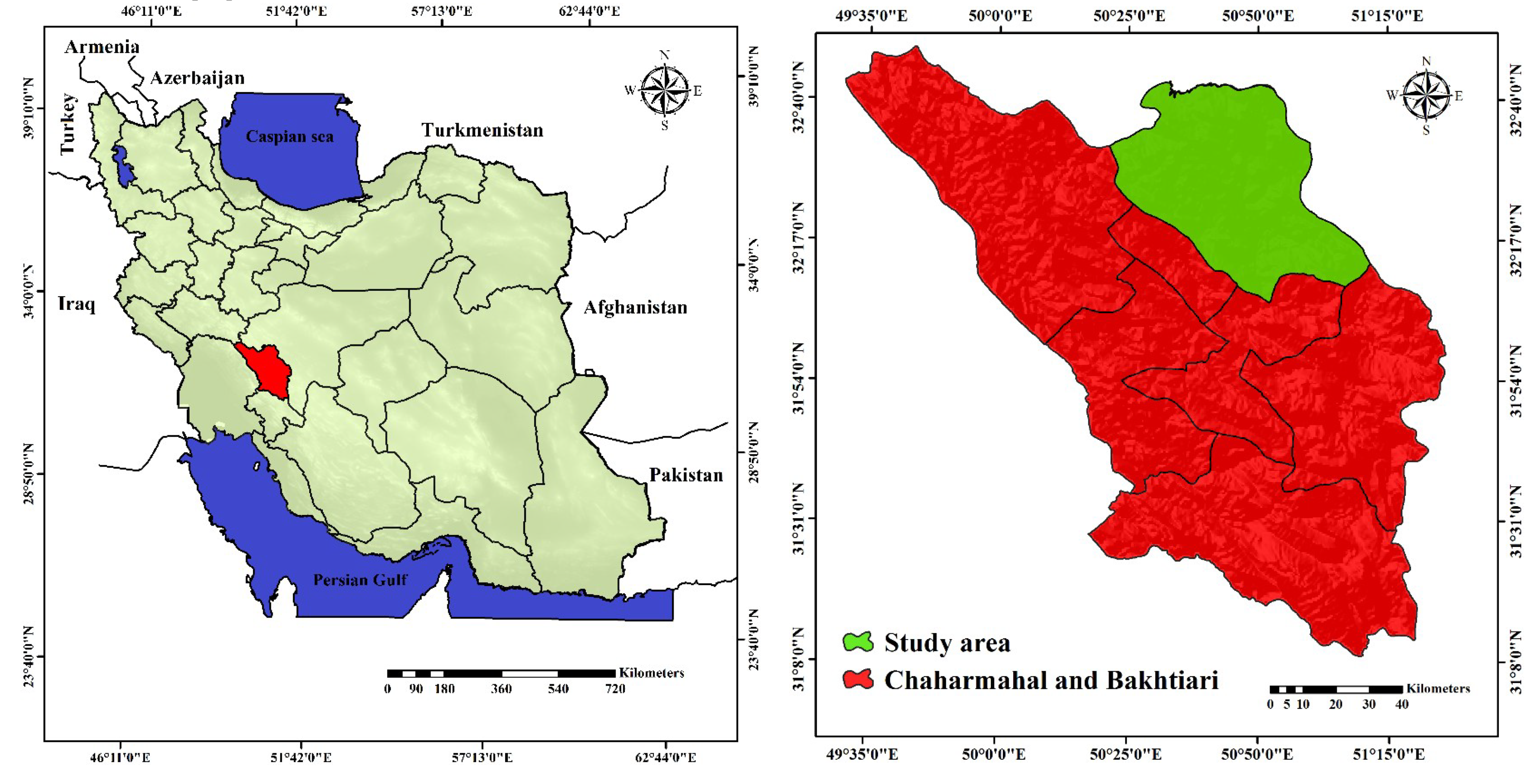
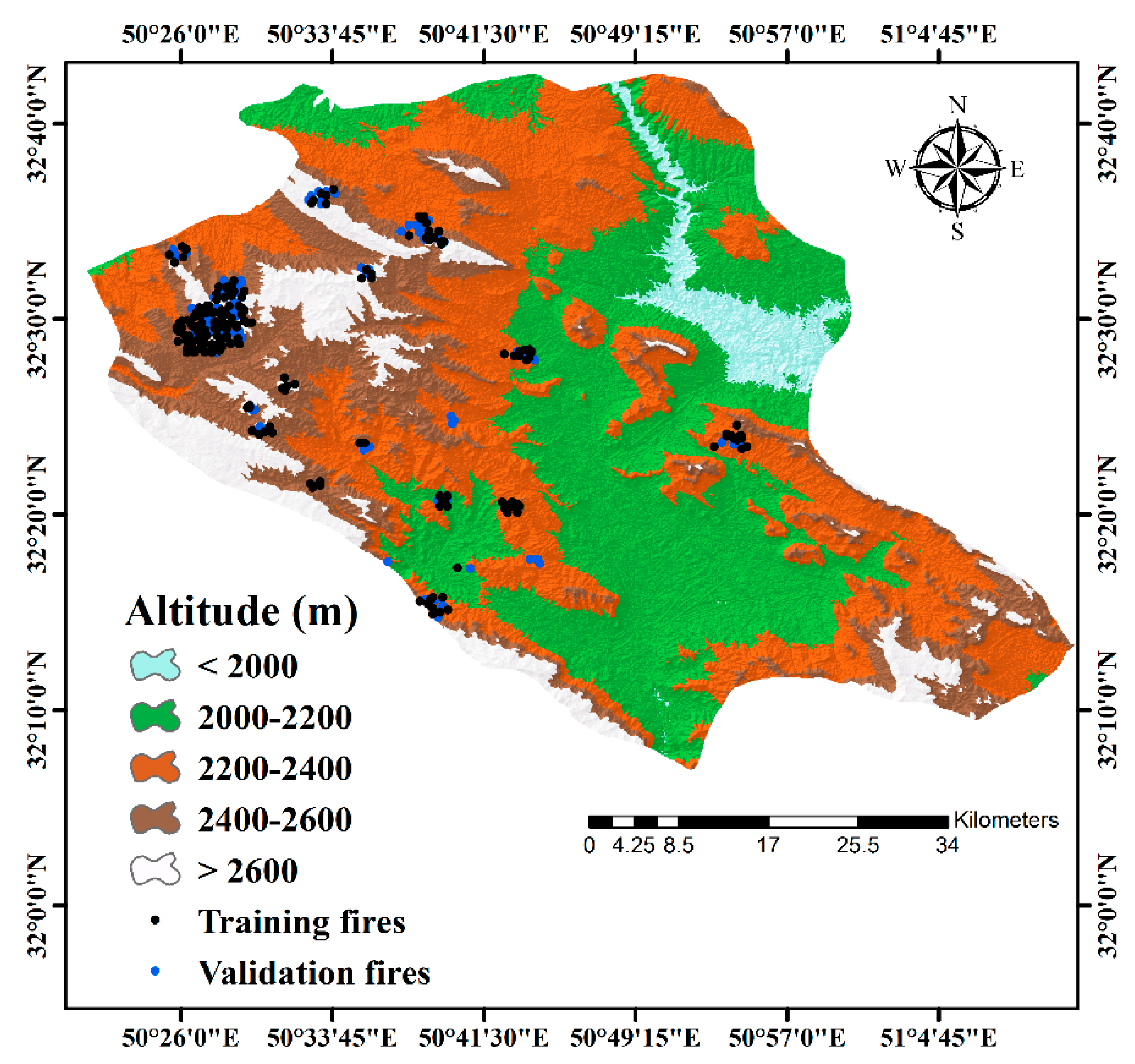
2.1. Study Area
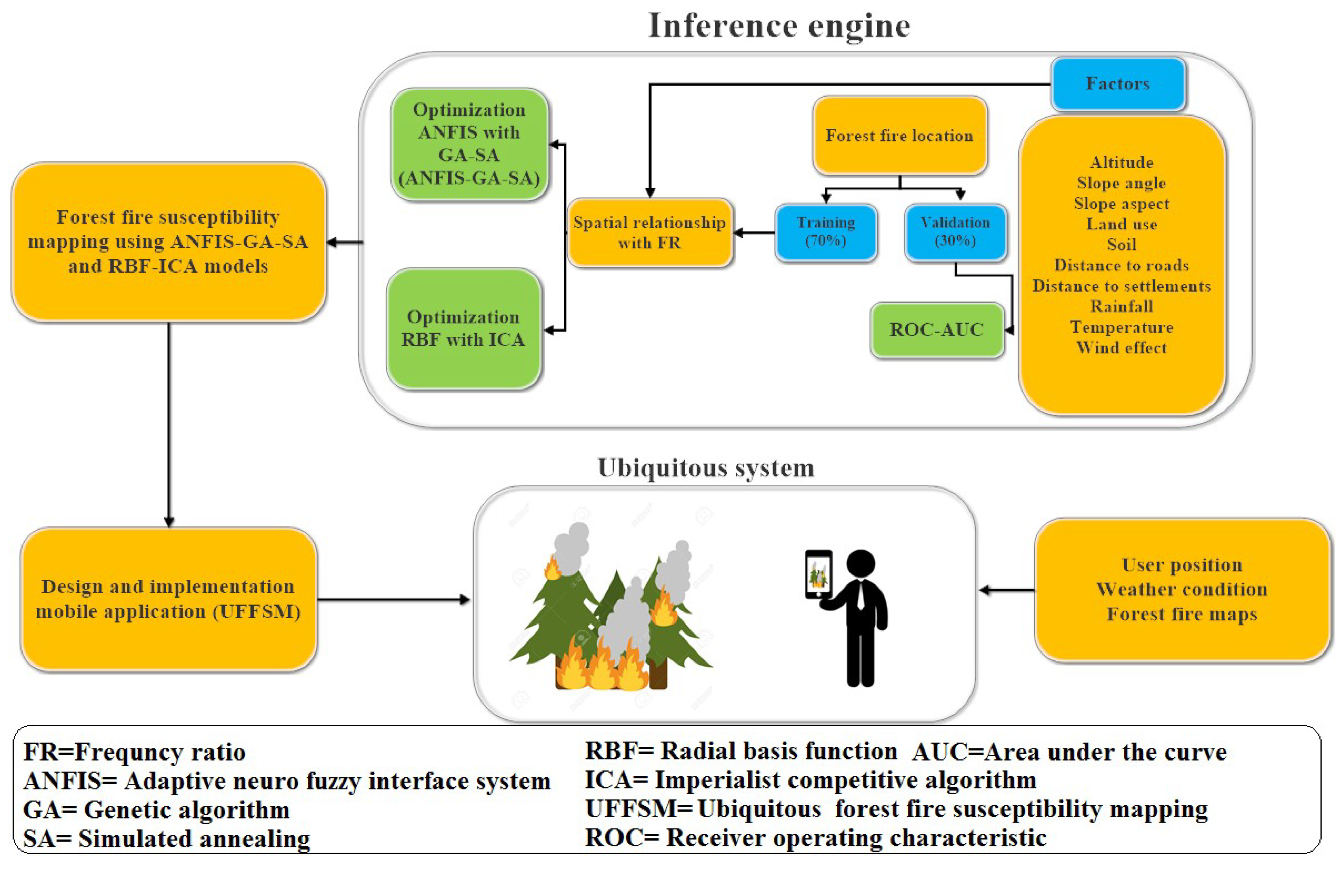
2.2. Methods
2.2.1. FR Model
2.2.2. ANFIS Model
2.2.3. GA Algorithm
2.2.4. SA Algorithm
2.2.5. ICA Algorithm
2.2.6. RBF Model
3. Research Framework
3.1. Spatial Database
3.1.1. Forest Fire Inventory
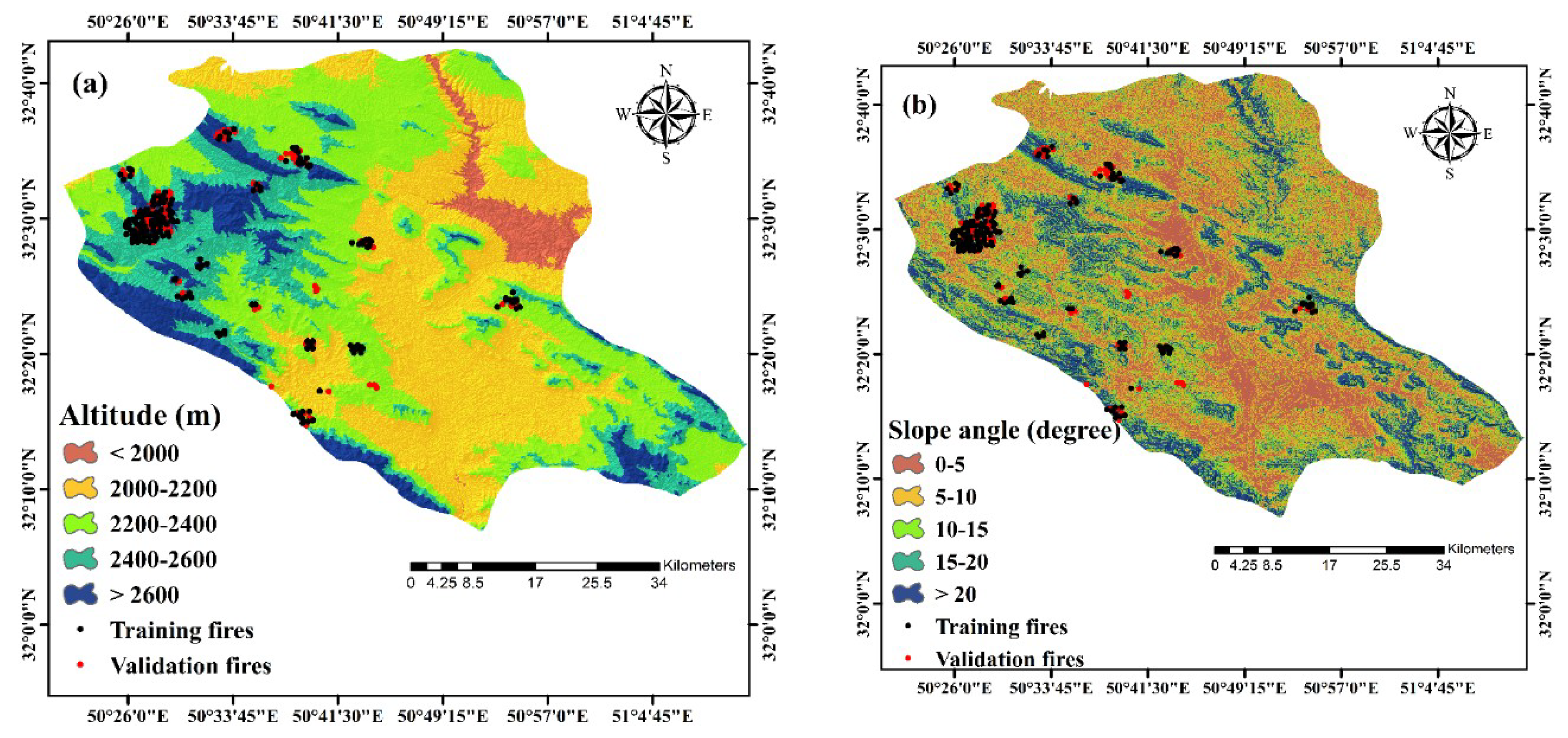
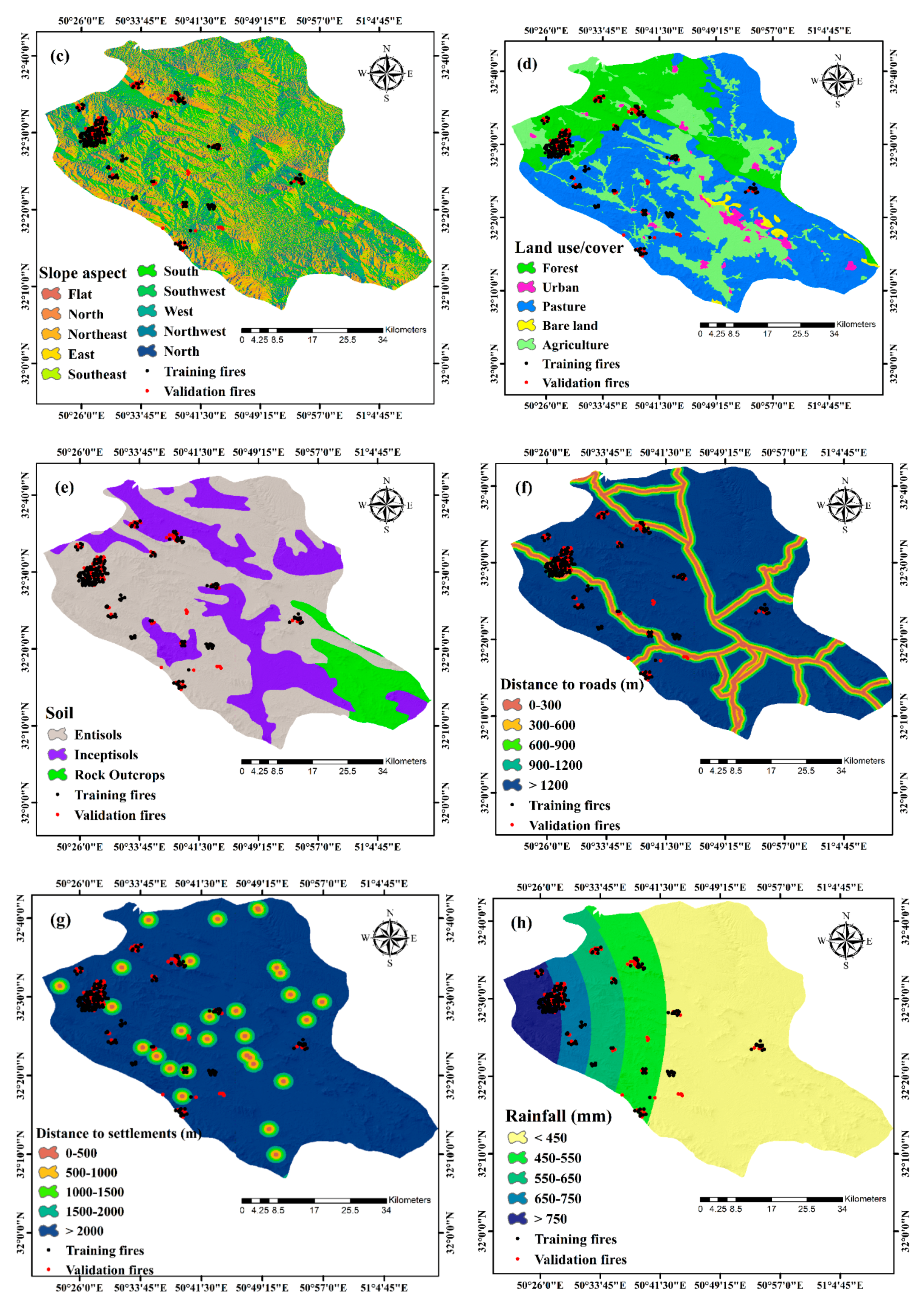
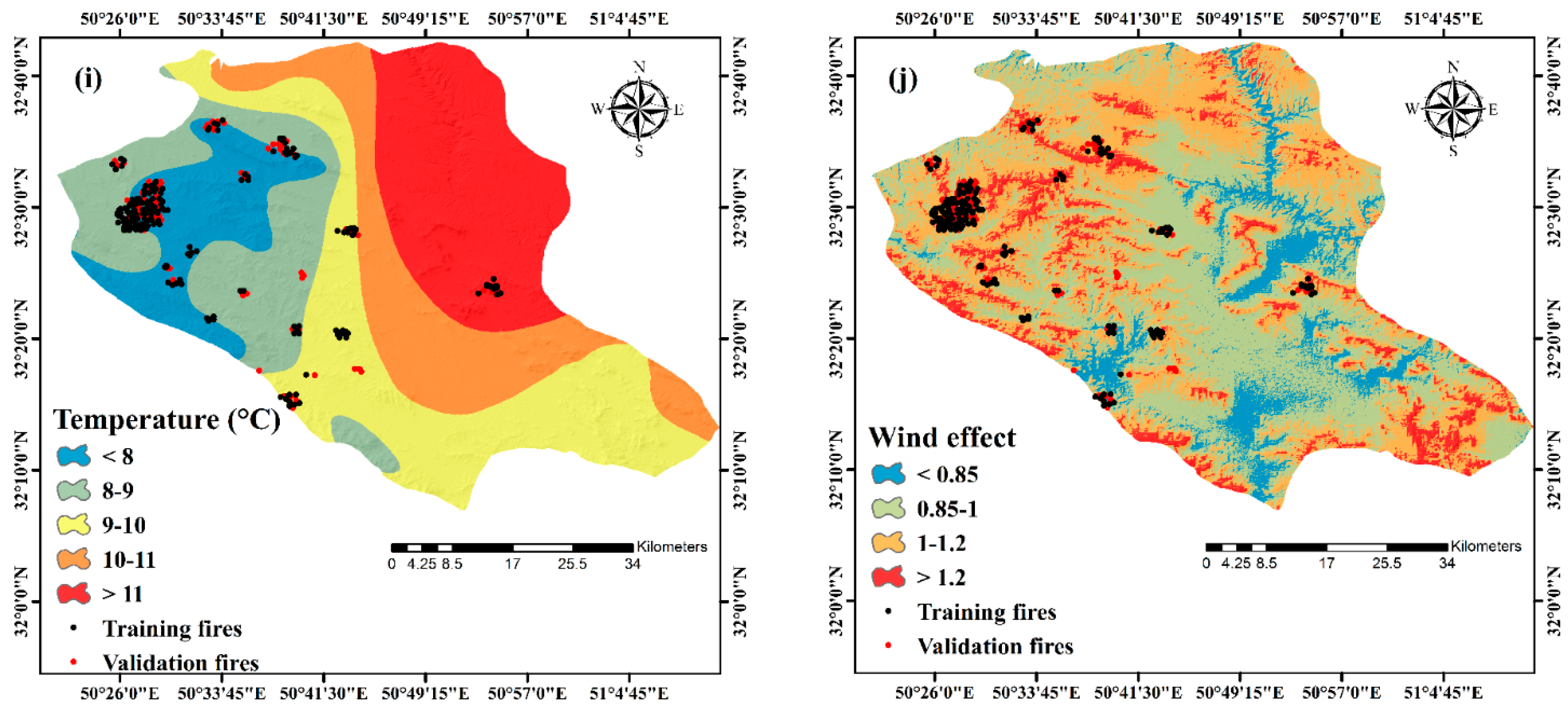
3.1.2. Criteria Affecting Forest Fire
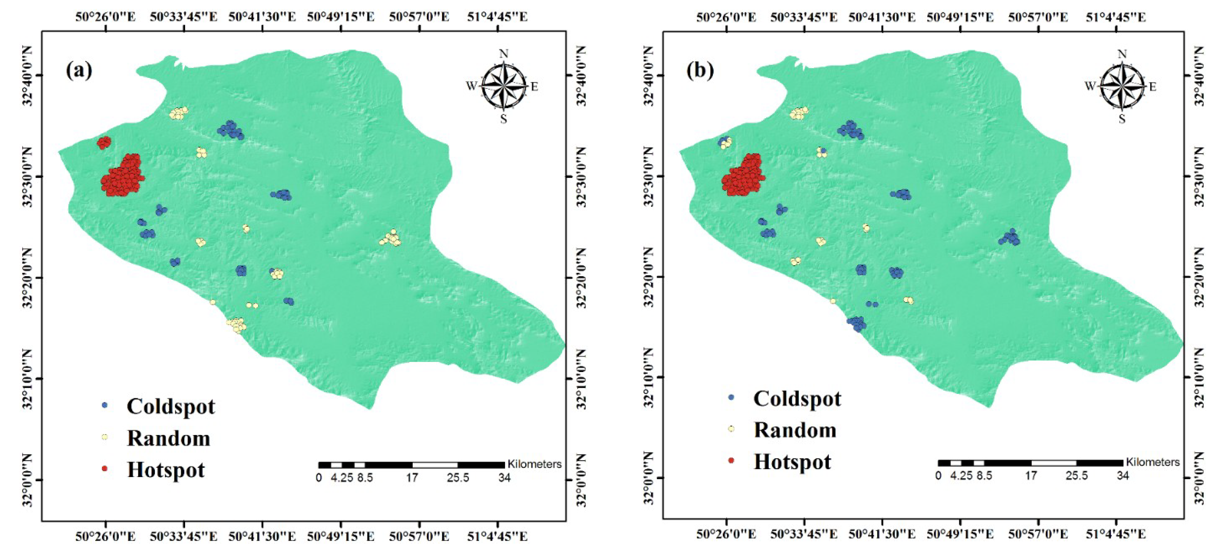
3.2. Analysis of Forest Fire Hotspot
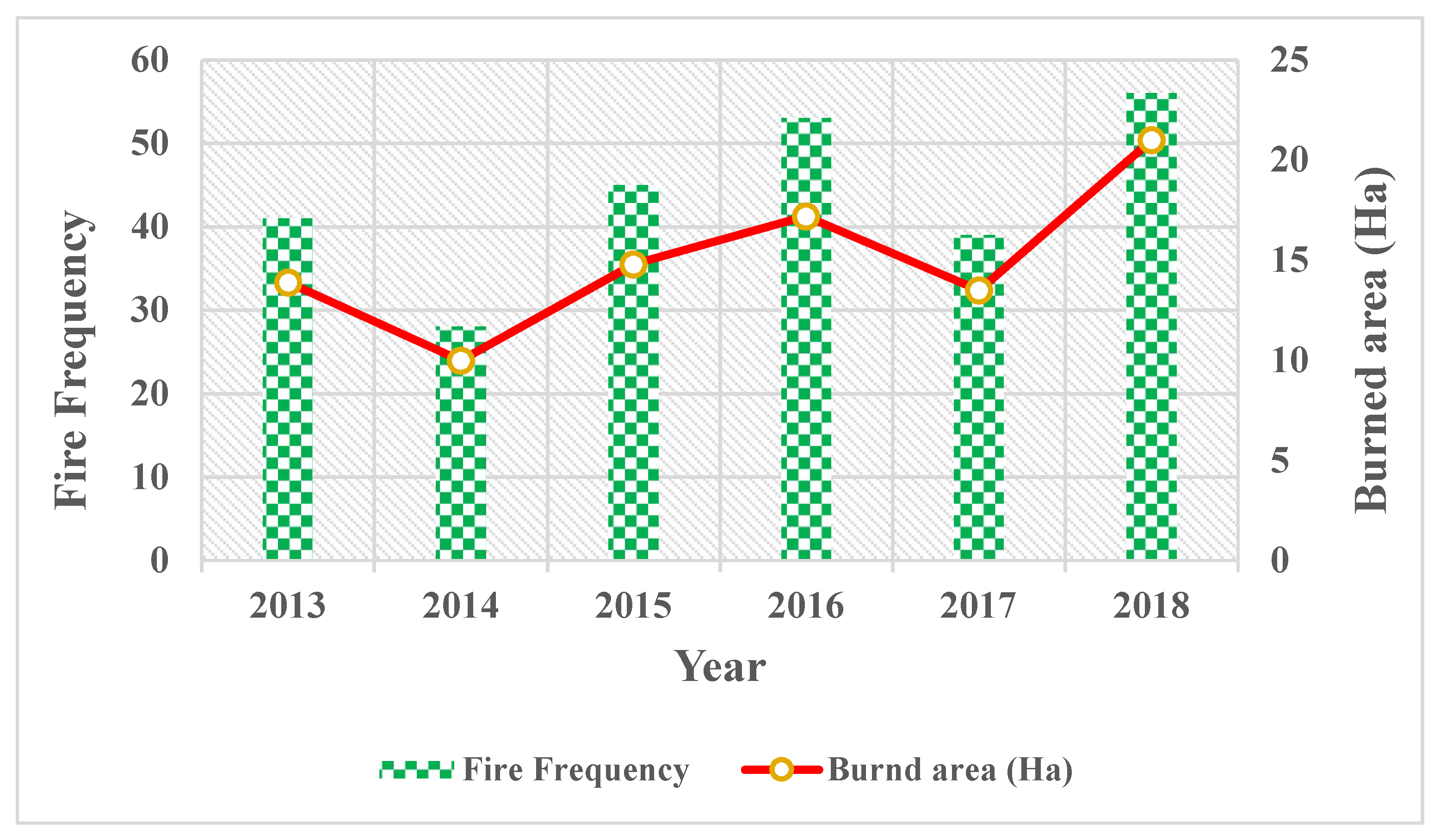
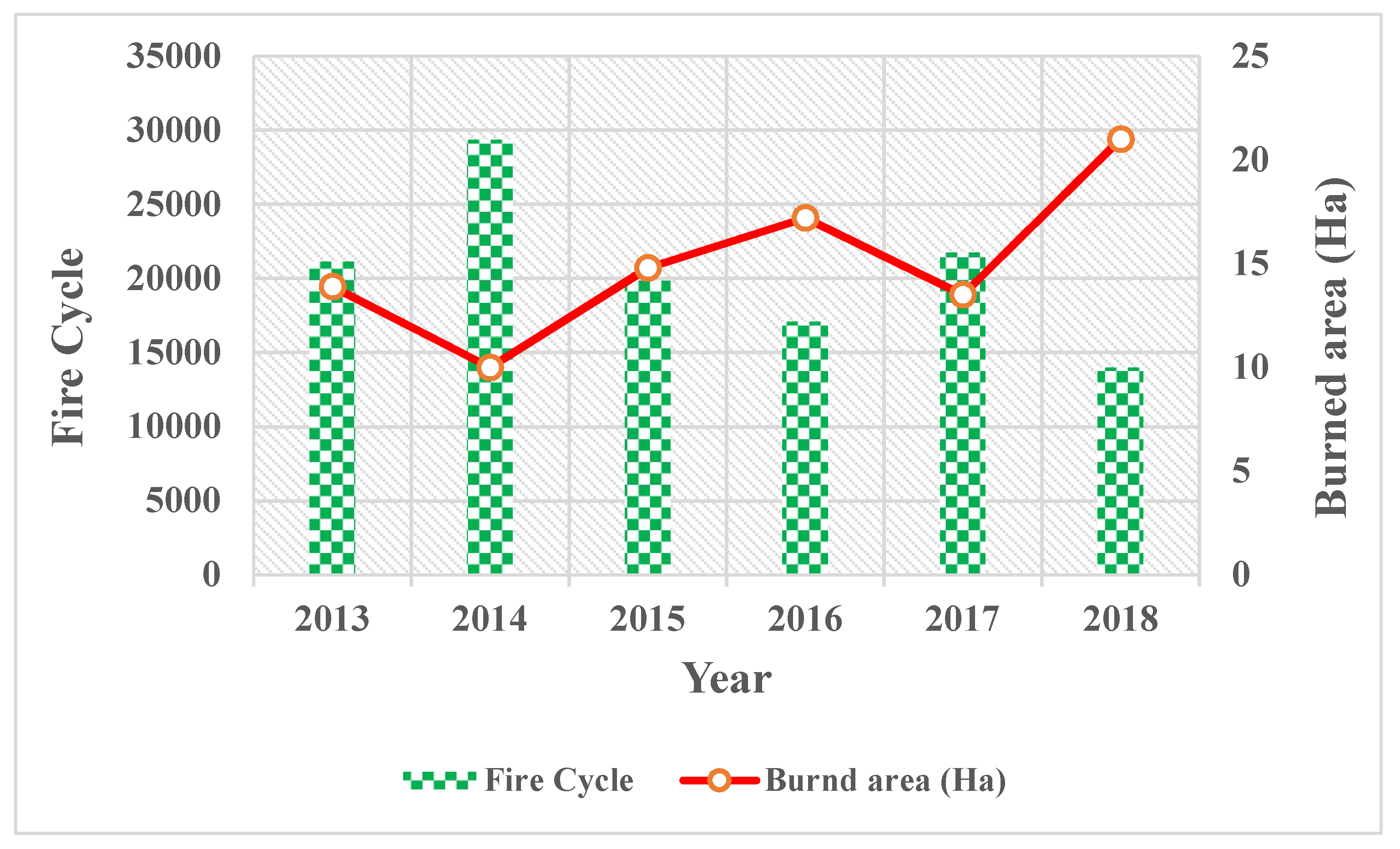
3.2.1. Analysis of Fire Frequency and Fire Cycle
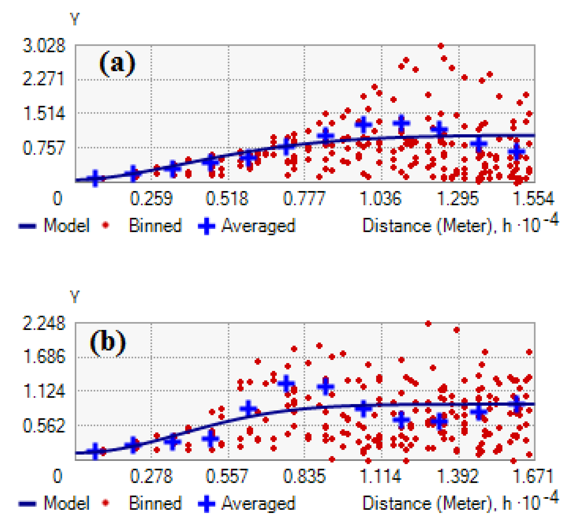
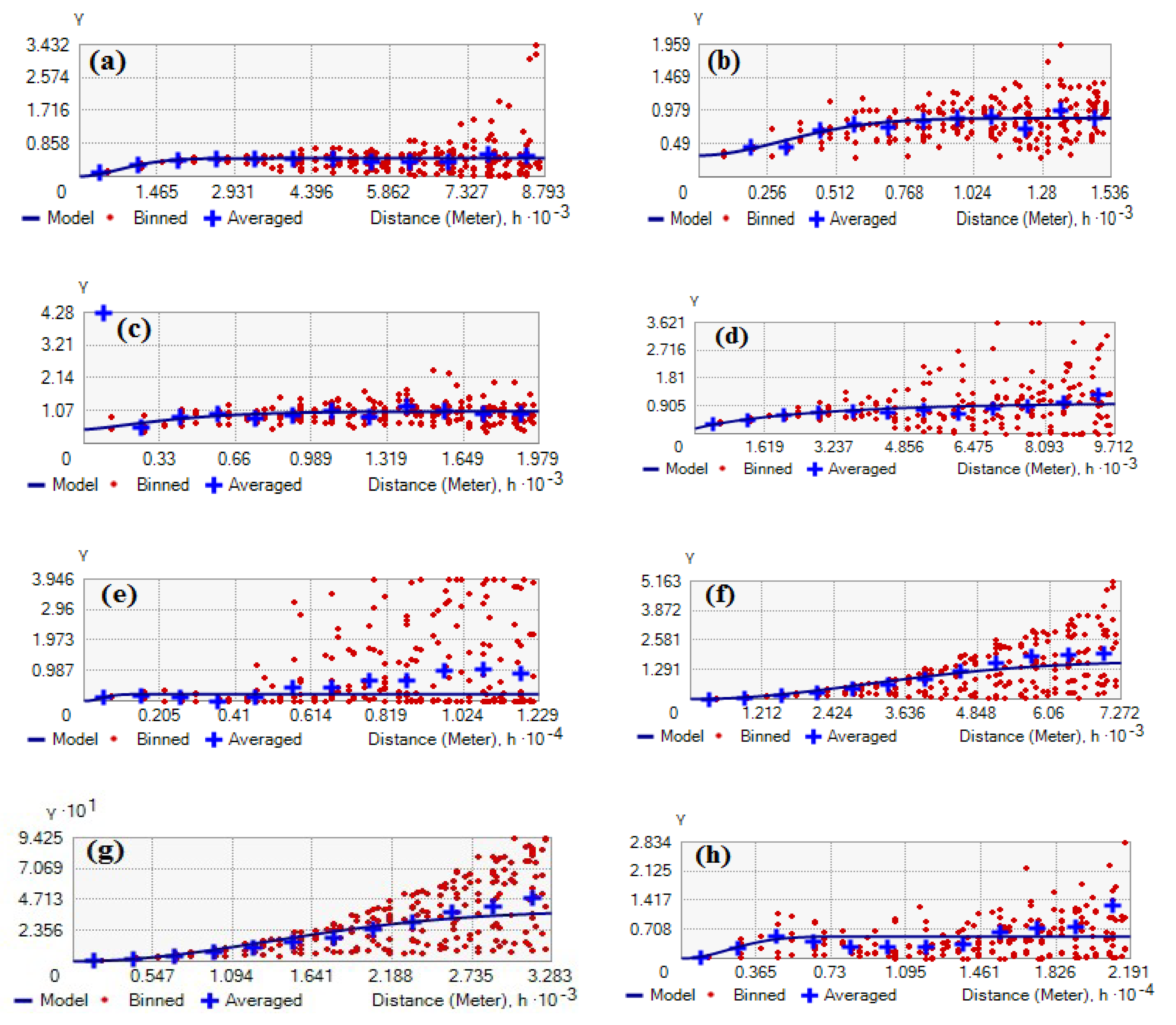
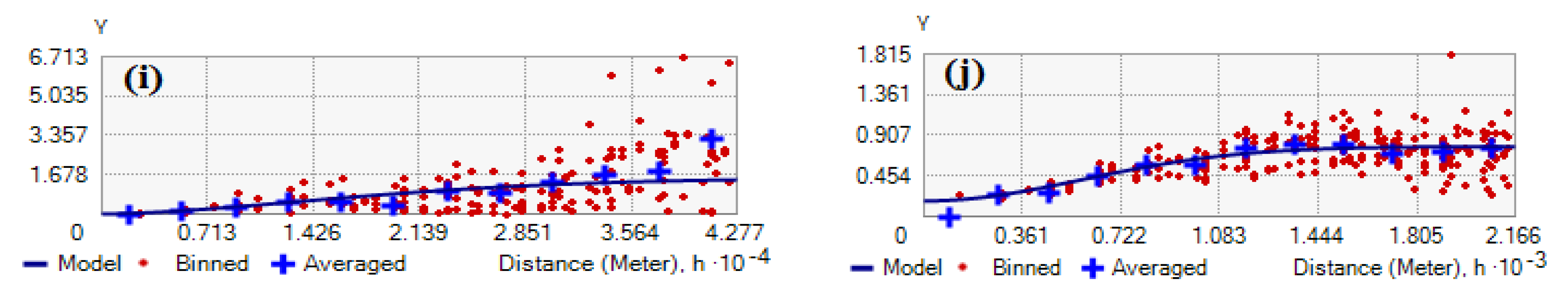
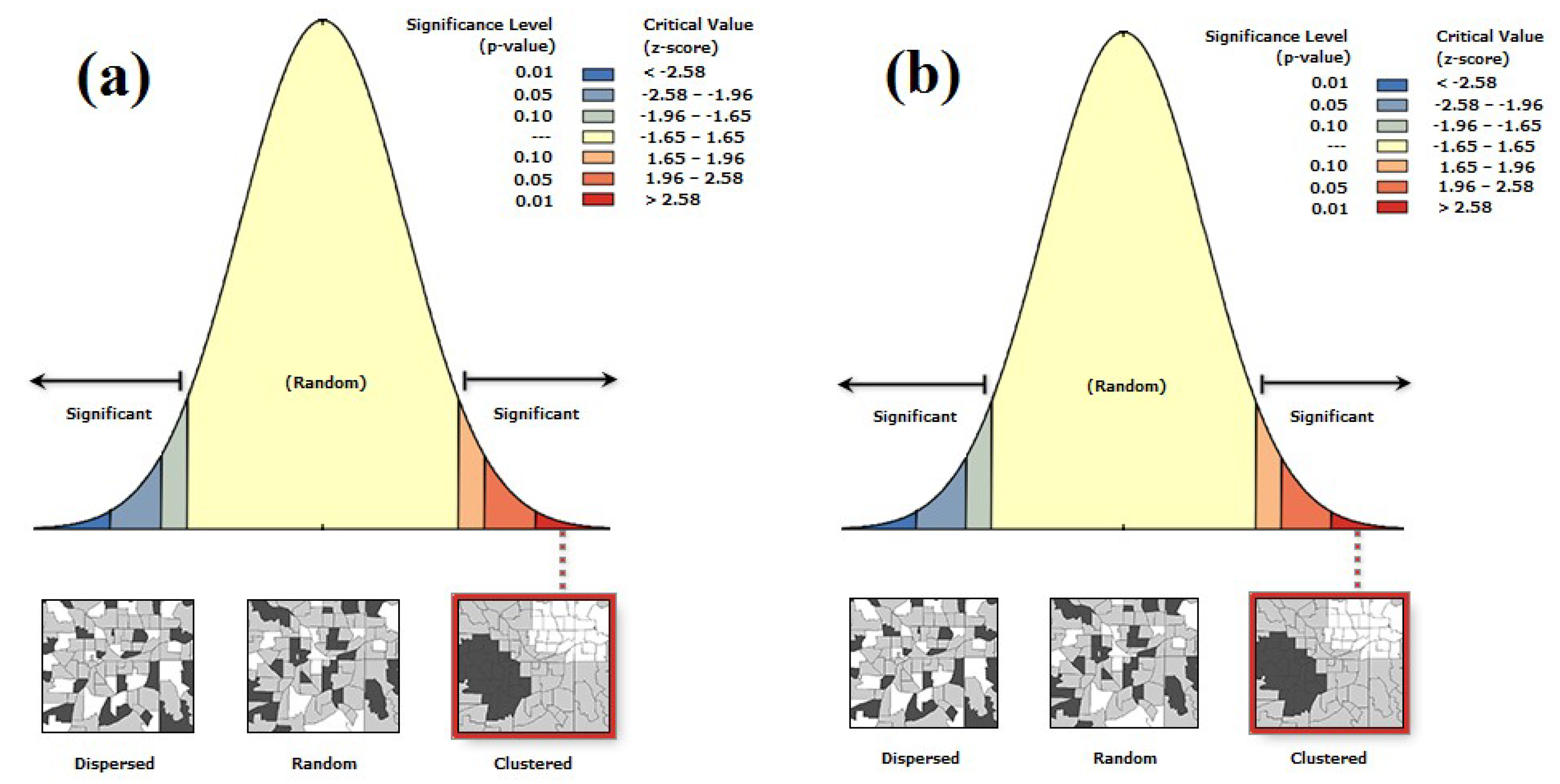
3.2.2. Spatial Autocorrelation Analysis
Semivariogram
Moran’s I Index
3.3. Combining ANFIS with Hybrid Algorithm
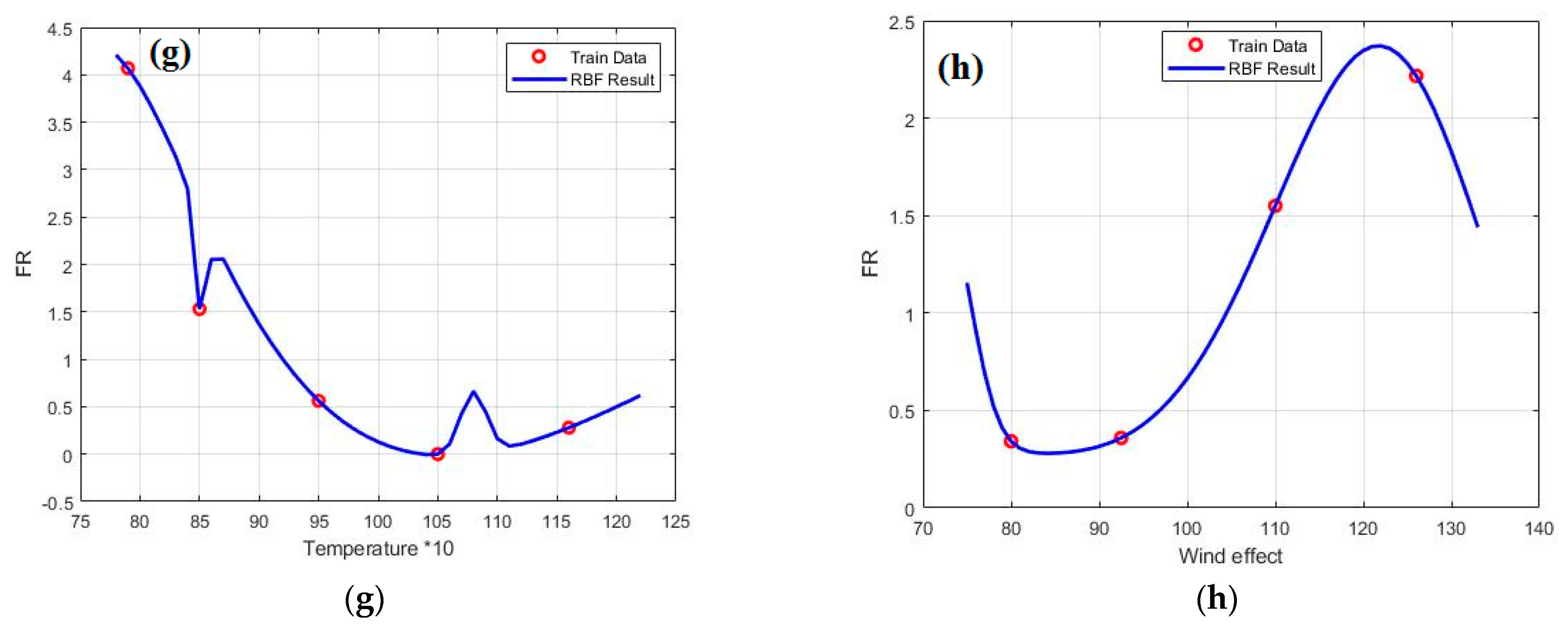
3.4. Combining RBF Interpolation Method with ICA Algorithm
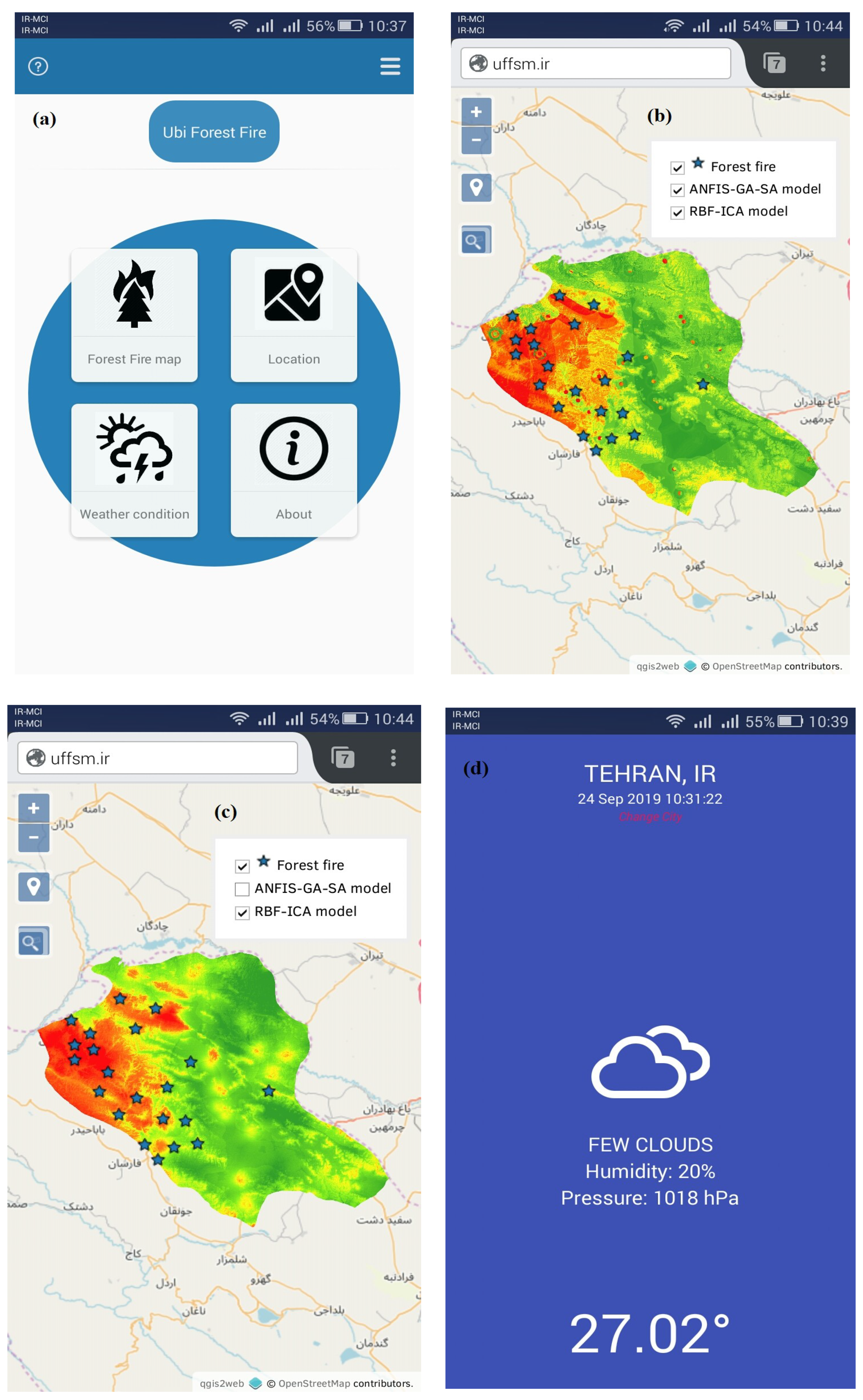
3.5. Ubiquitous GIS
3.6. Validation and Comparison
4. Results
4.1. Results of Forest Fire Hot Spot Analysis
4.2. Results of Spatial Autocorrelation
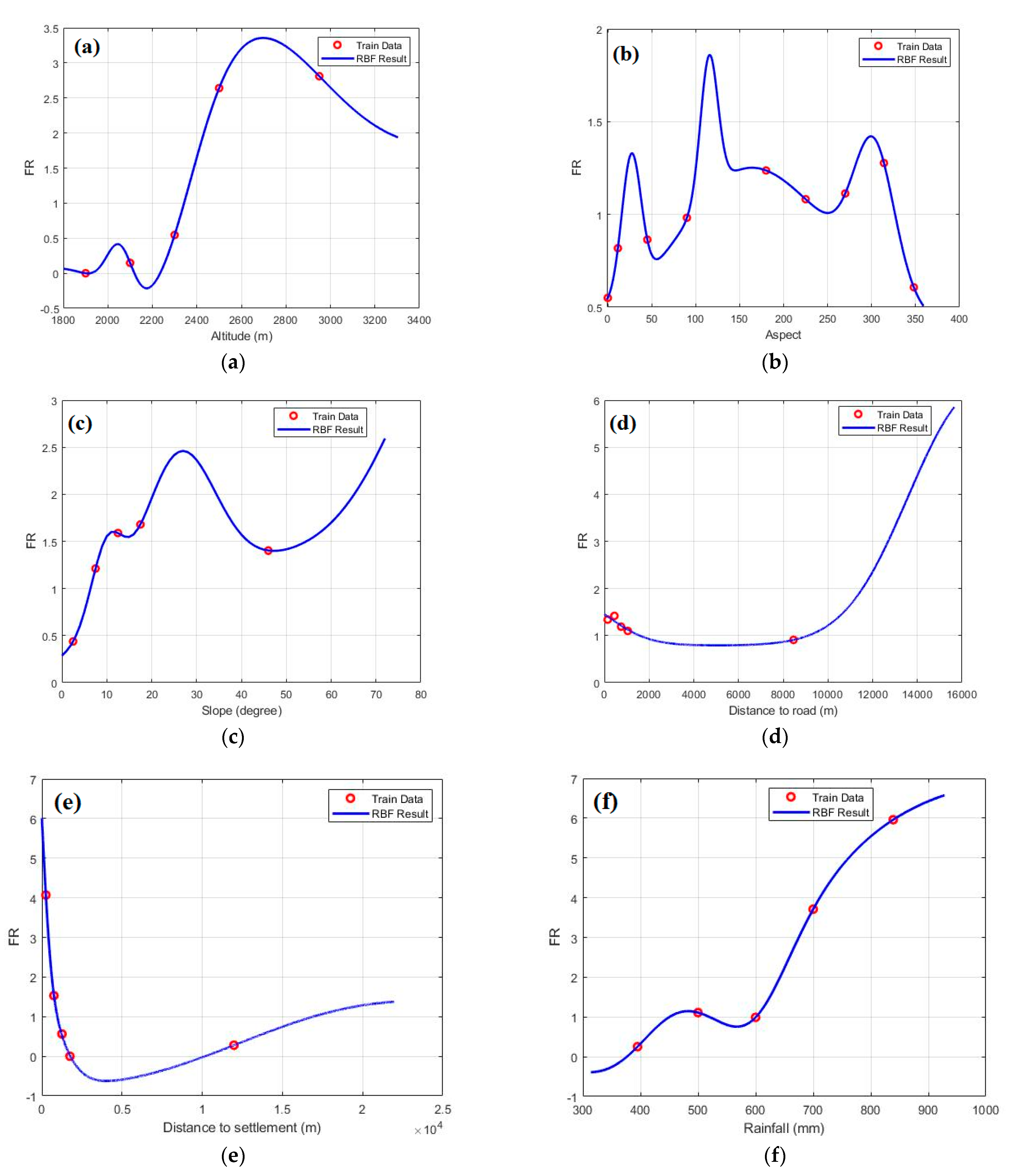
4.3. Results of FR
4.4. Results of the ANFIS-GA-SA Model
4.5. Results of RBF-ICA Model
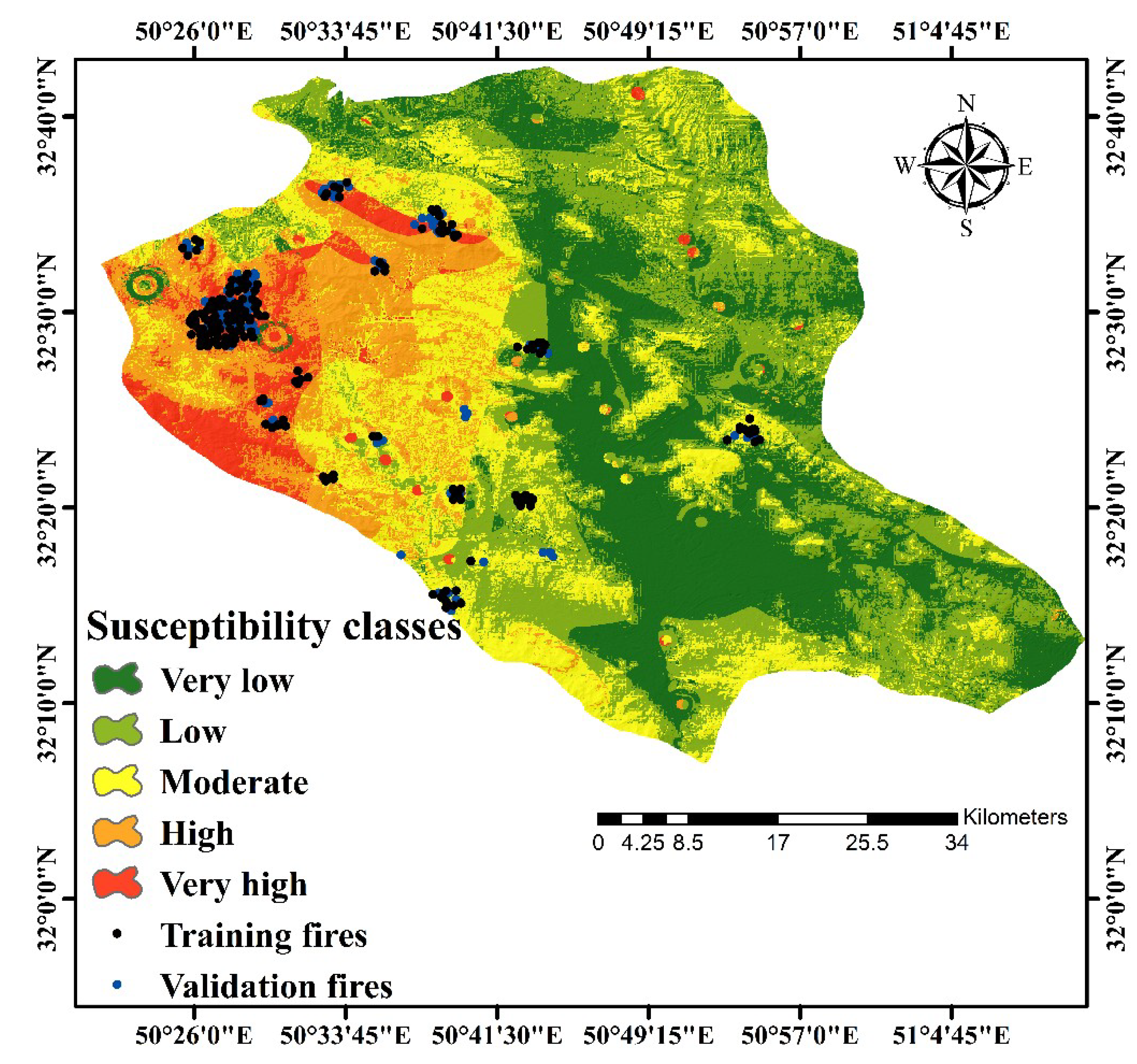
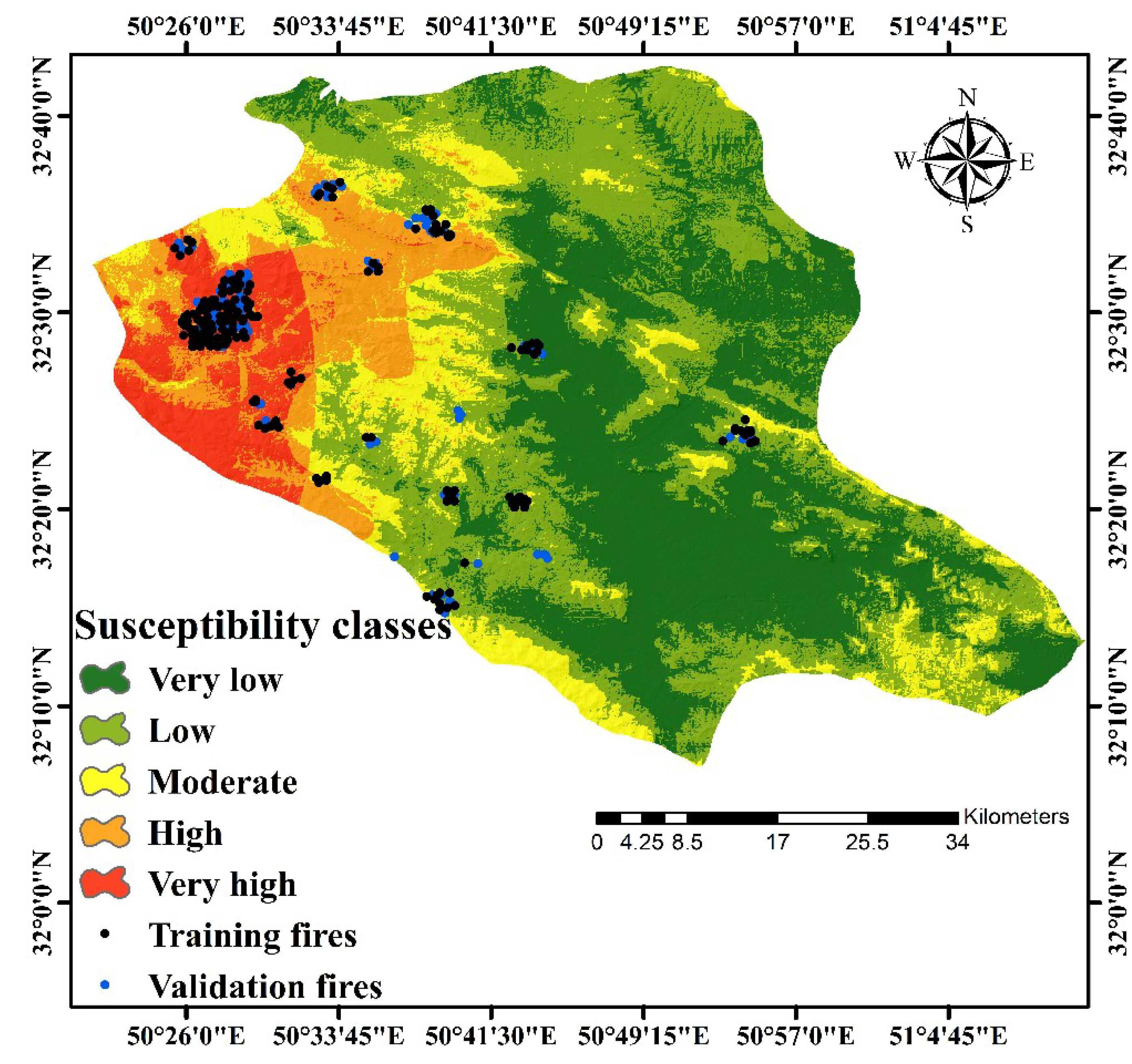
4.6. Results of a Ubiquitous GIS-Based FFSM
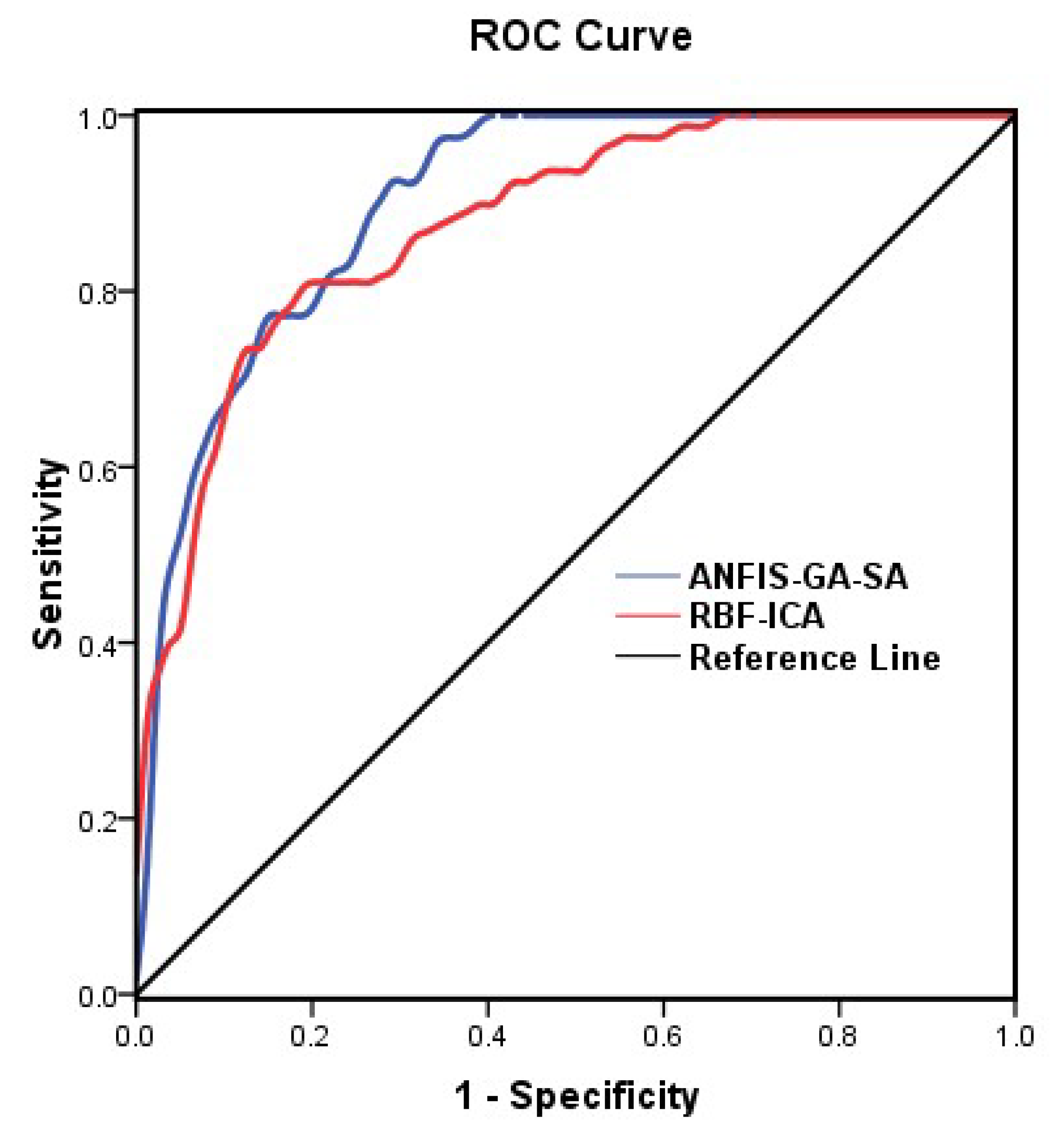
4.7. Results Validation
5. Discussion
6. Conclusions
Author Contributions
Funding
Conflicts of Interest
References
- Wali, M.K.; Watts, S.E. Forest ecology. J. Environ. Qual. 1999, 28, 1683–1685. [Google Scholar] [CrossRef]
- Jaafari, A.; Termeh, S.V.R.; Bui, D.T. Genetic and firefly metaheuristic algorithms for an optimized neuro-fuzzy prediction modeling of wildfire probability. J. Environ. Manag. 2019, 243, 358–369. [Google Scholar] [CrossRef] [PubMed]
- Yin, H.-W.; Kong, F.-H.; Li, X.-Z. Rs and gis-based forest fire risk zone mapping in da hinggan mountains. Chin. Geogr. Sci. 2004, 14, 251–257. [Google Scholar] [CrossRef]
- Ketterings, Q.M.; Wibowo, T.T.; van Noordwijk, M.; Penot, E. Farmers’ perspectives on slash-and-burn as a land clearing method for small-scale rubber producers in sepunggur, jambi province, sumatra, indonesia. For. Ecol. Manag. 1999, 120, 157–169. [Google Scholar] [CrossRef]
- Adab, H.; Kanniah, K.D.; Solaimani, K. Modeling forest fire risk in the northeast of iran using remote sensing and gis techniques. Nat. Hazards 2013, 65, 1723–1743. [Google Scholar] [CrossRef]
- Sarkargar Ardakani, A.; Valdan Zouj, M.; Mansoorian, A. Spatial analysis of fire potential in iran different region by using rs and gis. J. Environ. Sci. 2009, 35, 25–34. [Google Scholar]
- Jaafari, A.; Pourghasemi, H.R. Factors influencing regional-scale wildfire probability in iran: An application of random forest and support vector machine. In Spatial Modeling in GIS and R for Earth and Environmental Sciences; Elsevier: Amsterdam, The Netherlands, 2019; pp. 607–619. [Google Scholar]
- Adab, H.; Kanniah, K.D.; Solaimani, K.; Sallehuddin, R. Modelling static fire hazard in a semi-arid region using frequency analysis. Int. J. Wildland Fire 2015, 24, 763–777. [Google Scholar] [CrossRef]
- Pradhan, B.; Suliman, M.D.H.B.; Awang, M.A.B. Forest fire susceptibility and risk mapping using remote sensing and geographical information systems (gis). Disaster Prev. Manag. Int. J. 2007, 16. [Google Scholar] [CrossRef]
- Pourghasemi, H.R. Gis-based forest fire susceptibility mapping in iran: A comparison between evidential belief function and binary logistic regression models. Scand. J. For. Res. 2016, 31, 80–98. [Google Scholar] [CrossRef]
- Karimi, A.; Abdollahi, S.; Ostad-Ali-Askari, K.; Singh, V.P.; Eslamian, S.; Heidarian, A.; Nekooei, M.; Gholami, H.; Pazdar, S. Evaluating models and effective factors obtained from remote sensing (rs) and geographic information system (gis) in the prediction of forest fire risk, structured review. J. Geogr. Cartogr. 2018, 1. [Google Scholar] [CrossRef]
- Hong, H.; Naghibi, S.A.; Dashtpagerdi, M.M.; Pourghasemi, H.R.; Chen, W. A comparative assessment between linear and quadratic discriminant analyses (lda-qda) with frequency ratio and weights-of-evidence models for forest fire susceptibility mapping in china. Arab. J. Geosci. 2017, 10, 167. [Google Scholar] [CrossRef]
- Nami, M.; Jaafari, A.; Fallah, M.; Nabiuni, S. Spatial prediction of wildfire probability in the hyrcanian ecoregion using evidential belief function model and gis. Int. J. Environ. Sci. Technol. 2018, 15, 373–384. [Google Scholar] [CrossRef]
- Jaafari, A.; Gholami, D.M.; Zenner, E.K. A bayesian modeling of wildfire probability in the zagros mountains, iran. Ecol. Inform. 2017, 39, 32–44. [Google Scholar] [CrossRef]
- Gigović, L.; Pourghasemi, H.R.; Drobnjak, S.; Bai, S. Testing a new ensemble model based on svm and random forest in forest fire susceptibility assessment and its mapping in serbia’s tara national park. Forests 2019, 10, 408. [Google Scholar] [CrossRef]
- Sachdeva, S.; Bhatia, T.; Verma, A. Gis-based evolutionary optimized gradient boosted decision trees for forest fire susceptibility mapping. Natural Hazards 2018, 92, 1399–1418. [Google Scholar] [CrossRef]
- Bui, D.T.; Bui, Q.-T.; Nguyen, Q.-P.; Pradhan, B.; Nampak, H.; Trinh, P.T. A hybrid artificial intelligence approach using gis-based neural-fuzzy inference system and particle swarm optimization for forest fire susceptibility modeling at a tropical area. Agric. For. Meteorol. 2017, 233, 32–44. [Google Scholar]
- Pourtaghi, Z.S.; Pourghasemi, H.R.; Aretano, R.; Semeraro, T. Investigation of general indicators influencing on forest fire and its susceptibility modeling using different data mining techniques. Ecol. Indic. 2016, 64, 72–84. [Google Scholar] [CrossRef]
- Dimuccio, L.A.; Ferreira, R.; Cunha, L.; de Almeida, A.C. Regional forest-fire susceptibility analysis in central portugal using a probabilistic ratings procedure and artificial neural network weights assignment. Int. J. Wildland Fire 2011, 20, 776–791. [Google Scholar] [CrossRef]
- Suryabhagavan, K.; Alemu, M.; Balakrishnan, M. Gis-based multi-criteria decision analysis for forest fire susceptibility mapping: A case study in harenna forest, southwestern ethiopia. Trop. Ecol. 2016, 57, 33–43. [Google Scholar]
- Lv, Z.; Réhman, S.U.; Chen, G. Webvrgis: A p2p Network Engine for VR Data and GIS Analysis. In Proceedings of the International Conference on Neural Information Processing, Daegu, Germany, 3–7 November 2013; Springer: Berlin/Heidelberg, Germany; pp. 503–510. [Google Scholar]
- Debevec, P.E.; Taylor, C.J.; Malik, J. Modeling and rendering architecture from photographs: A hybrid geometry-and image-based approach. In Proceedings of the 23rd Annual Conference on Computer Graphics and Interactive Techniques, New Orleans, LA, USA, 4–9 August 1996; pp. 11–20. [Google Scholar]
- Kim, S.K.; Lee, J.H.; Ryu, K.H.; Kim, U. A framework of spatial co-location pattern mining for ubiquitous gis. Multimed. Tools Appl. 2014, 71, 199–218. [Google Scholar] [CrossRef]
- Jaafari, A.; Zenner, E.K.; Panahi, M.; Shahabi, H. Hybrid artificial intelligence models based on a neuro-fuzzy system and metaheuristic optimization algorithms for spatial prediction of wildfire probability. Agric. For. Meteorol. 2019, 266, 198–207. [Google Scholar] [CrossRef]
- Dong, C.; Liu, F.; Wang, H.; Chen, F. Application Research of Mobile GIS in Forestry Informatization. In Proceedings of the 5th International Conference on Computer Science & Education, Hefei, China, NJ, USA, 24–27 August 2010; IEEE: Piscataway, NJ, USA; pp. 351–355. [Google Scholar]
- Battad, D.; Mackenzie, P. Applications of mobile gis in forestry south australia. Int. Arch. Photogramm. Remote Sens. Spat. Inf. Sci. 2012, 39, 447–452. [Google Scholar] [CrossRef]
- Kalabokidis, K.; Athanasis, N.; Gagliardi, F.; Karayiannis, F.; Palaiologou, P.; Parastatidis, S.; Vasilakos, C. Virtual fire: A web-based gis platform for forest fire control. Ecol. Inform. 2013, 16, 62–69. [Google Scholar] [CrossRef]
- Roberto Barbosa, M.; Carlos Sicoli Seoane, J.; Guimaraes Buratto, M.; Santana de Oliveira Dias, L.; Paulo Carvalho Raivel, J.; Lobos Martins, F. Forest fire alert system: A geo web gis prioritization model considering land susceptibility and hotspots—A case study in the carajás national forest, brazilian amazon. Int. J. Geogr. Inf. Sci. 2010, 24, 873–901. [Google Scholar] [CrossRef]
- Jeefoo, P. Wildfire field survey using mobile GIS technology in Nan province. In Proceedings of the 2019 Joint International Conference on Digital Arts, Media and Technology with ECTI Northern Section Conference on Electrical, Electronics, Computer and Telecommunications Engineering (ECTI DAMT-NCON), Nan, Thailand, 30 January–2 February 2019; IEEE: Piscataway, NJ, USA, 2019; pp. 98–100. [Google Scholar]
- Moayedi, H.; Mehrabi, M.; Bui, D.T.; Pradhan, B.; Foong, L.K. Fuzzy-metaheuristic ensembles for spatial assessment of forest fire susceptibility. J. Environ. Manag. 2020, 260, 109867. [Google Scholar] [CrossRef] [PubMed]
- Hong, H.; Tsangaratos, P.; Ilia, I.; Liu, J.; Zhu, A.-X.; Xu, C. Applying genetic algorithms to set the optimal combination of forest fire related variables and model forest fire susceptibility based on data mining models. The case of dayu county, china. Sci. Total Environ. 2018, 630, 1044–1056. [Google Scholar] [CrossRef]
- Zhang, G.; Wang, M.; Liu, K. Forest fire susceptibility modeling using a convolutional neural network for yunnan province of china. Int. J. Disaster Risk Sci. 2019, 10, 386–403. [Google Scholar] [CrossRef]
- Bui, Q.-T. Metaheuristic algorithms in optimizing neural network: A comparative study for forest fire susceptibility mapping in dak nong, vietnam. Geomat. Nat. Hazards Risk 2019, 10, 136–150. [Google Scholar] [CrossRef]
- Jaafari, A.; Najafi, A.; Pourghasemi, H.; Rezaeian, J.; Sattarian, A. Gis-based frequency ratio and index of entropy models for landslide susceptibility assessment in the caspian forest, northern iran. Int. J. Environ. Sci. Technol. 2014, 11, 909–926. [Google Scholar] [CrossRef]
- Jang, J.-S. Anfis: Adaptive-network-based fuzzy inference system. IEEE Trans. Syst. Manand Cybern. 1993, 23, 665–685. [Google Scholar] [CrossRef]
- Yaghoobi, A.; Bakhshi-Jooybari, M.; Gorji, A.; Baseri, H. Application of adaptive neuro fuzzy inference system and genetic algorithm for pressure path optimization in sheet hydroforming process. Int. J. Adv. Manuf. Technol. 2016, 86, 2667–2677. [Google Scholar] [CrossRef]
- Sivanandam, S.; Deepa, S. Genetic algorithms. In Introduction to Genetic Algorithms; Springer: Berlin/Heidelberg, Germany, 2008; pp. 15–37. [Google Scholar]
- Mukhopadhyay, D.M.; Balitanas, M.O.; Farkhod, A.; Jeon, S.-H.; Bhattacharyya, D. Genetic algorithm: A tutorial review. Int. J. Grid Distrib. Comput. 2009, 2, 25–32. [Google Scholar]
- Ravagnani, M.; Silva, A.; Arroyo, P.; Constantino, A. Heat exchanger network synthesis and optimisation using genetic algorithm. Appl. Therm. Eng. 2005, 25, 1003–1017. [Google Scholar] [CrossRef]
- Kirkpatrick, S.; Gelatt, C.D.; Vecchi, M.P. Optimization by simulated annealing. Science 1983, 220, 671–680. [Google Scholar] [CrossRef]
- Misevičius, A. A modified simulated annealing algorithm for the quadratic assignment problem. Informatica 2003, 14, 497–514. [Google Scholar] [CrossRef]
- Dudek, G. Adaptive simulated annealing schedule to the unit commitment problem. Electr. Power Syst. Res. 2010, 80, 465–472. [Google Scholar] [CrossRef]
- Atashpaz-Gargari, E.; Lucas, C. Imperialist competitive algorithm: An algorithm for optimization inspired by imperialistic competition. In Proceedings of the IEEE Congress on Evolutionary Computation, Singapore, 25–28 September 2007; IEEE: Piscataway, NJ, USA; pp. 4661–4667. [Google Scholar]
- Talatahari, S.; Azar, B.F.; Sheikholeslami, R.; Gandomi, A. Imperialist competitive algorithm combined with chaos for global optimization. Commun. Nonlinear Sci. Numer. Simul. 2012, 17, 1312–1319. [Google Scholar] [CrossRef]
- Schueremans, L.; Van Gemert, D. Benefit of splines and neural networks in simulation based structural reliability analysis. Struct. Saf. 2005, 27, 246–261. [Google Scholar] [CrossRef]
- Jaiswal, R.K.; Mukherjee, S.; Raju, K.D.; Saxena, R. Forest fire risk zone mapping from satellite imagery and gis. Int. J. Appl. Earth Obs. Geoinf. 2002, 4, 1–10. [Google Scholar] [CrossRef]
- Chuvieco, E.; Congalton, R.G. Application of remote sensing and geographic information systems to forest fire hazard mapping. Remote Sens. Environ. 1989, 29, 147–159. [Google Scholar] [CrossRef]
- Vadrevu, K.P.; Eaturu, A.; Badarinath, K. Fire risk evaluation using multicriteria analysis—A case study. Environ. Monit. Assess. 2010, 166, 223–239. [Google Scholar] [CrossRef] [PubMed]
- Chandra, S. Application of remote sensing and gis technology in forest fire risk modeling and management of forest fires: A case study in the garhwal himalayan region. In Geo-Information for Disaster Management; Springer: Berlin/Heidelberg, Germany, 2005; pp. 1239–1254. [Google Scholar]
- Eskandari, S.; Chuvieco, E. Fire danger assessment in iran based on geospatial information. Int. J. Appl. Earth Obs. Geoinf. 2015, 42, 57–64. [Google Scholar] [CrossRef]
- Perera, A.H.; Euler, D.L.; Thompson, I.D. Ecology of a Managed Terrestrial Landscape: Patterns and Processes of Forest Landscapes in Ontario; UBC Press: Vancouver, BC, USA, 2011. [Google Scholar]
- Lim, C.-H.; Kim, Y.S.; Won, M.; Kim, S.J.; Lee, W.-K. Can satellite-based data substitute for surveyed data to predict the spatial probability of forest fire? A geostatistical approach to forest fire in the republic of korea. Geomat. Nat. Hazards Risk 2019, 10, 719–739. [Google Scholar] [CrossRef]
- Webster, R.; Oliver, M.A. Geostatistics for Environmental Scientists; John Wiley & Sons: Hoboken, NJ, USA, 2007. [Google Scholar]
- Gunnarsson, F.; Holm, S.; Holmgren, P.; Thuresson, T. On the potential of kriging for forest management planning. Scand. J. For. Res. 1998, 13, 237–245. [Google Scholar] [CrossRef]
- Ziegel, E.R. Geostatistics for environmental scientists. Technometrics 2001, 43, 499. [Google Scholar]
- Anselin, L. Local indicators of spatial association—Lisa. Geogr. Anal. 1995, 27, 93–115. [Google Scholar] [CrossRef]
- Getis, A.; Ord, J. The analysis of spatial association by use of distance statistics, geographycal analysis. In Perspectives on Spatial Data Analysis; Springer: Berlin/Heidelberg, Germany, 1992. [Google Scholar]
- Odland, J. Spatial Autocorrelation; SAGE Publications, Incorporated: New York, NY, USA, 1988; Volume 9. [Google Scholar]
- Haznedar, B.; Kalinli, A. Training anfis using genetic algorithm for dynamic systems identification. Int. J. Intell. Syst. Appl. Eng. 2016, 44–47. [Google Scholar] [CrossRef]
- Sarkheyli, A.; Zain, A.M.; Sharif, S. Robust optimization of anfis based on a new modified ga. Neurocomputing 2015, 166, 357–366. [Google Scholar] [CrossRef]
- Yu, H.; Fang, H.; Yao, P.; Yuan, Y. A combined genetic algorithm/simulated annealing algorithm for large scale system energy integration. Comput. Chem. Eng. 2000, 24, 2023–2035. [Google Scholar] [CrossRef]
- Termeh, S.V.R.; Kornejady, A.; Pourghasemi, H.R.; Keesstra, S. Flood susceptibility mapping using novel ensembles of adaptive neuro fuzzy inference system and metaheuristic algorithms. Sci. Total Environ. 2018, 615, 438–451. [Google Scholar] [CrossRef]
- Aghdam, I.N.; Varzandeh, M.H.M.; Pradhan, B. Landslide susceptibility mapping using an ensemble statistical index (wi) and adaptive neuro-fuzzy inference system (anfis) model at alborz mountains (iran). Environ. Earth Sci. 2016, 75, 553. [Google Scholar] [CrossRef]
- Weiser, M. The computer for the 21 st century. Sci. Am. 1991, 265, 94–105. [Google Scholar] [CrossRef]
- Krumm, J. Ubiquitous Computing Fundamentals; Chapman and Hall/CRC: Boca Raton, FL, USA, 2016. [Google Scholar]
- Truong, H.; Dustdar, S. Context coupling techniques. In Enabling Context-Aware Web Services: Methods, Architectures, and Technologies; Chapman and Hall/CRC: Boca Raton, FL, USA, 2010; pp. 337–364. [Google Scholar]
- Li, K.-J. Ubiquitous GIS, Part I: Basic Concepts of Ubiquitous GIS; Lecture Slides, Pusan National University: Busan, Korea, 2007. [Google Scholar]
- Razavi Termeh, V.; Sadeghi Niaraki, A. Design and implementation of ubiquitous health system (u-health) using smart-watches sensors. Int. Arch. Photogramm. Remote Sens. Spat. Inf. Sci. 2015, 40, 607–612. [Google Scholar] [CrossRef]
- Razavi-Termeh, S.V.; Sadeghi-Niaraki, A.; Choi, S.-M. Groundwater potential mapping using an integrated ensemble of three bivariate statistical models with random forest and logistic model tree models. Water 2019, 11, 1596. [Google Scholar] [CrossRef]
- Razavi-Termeh, S.V.; Sadeghi-Niaraki, A.; Choi, S.-M. Gully erosion susceptibility mapping using artificial intelligence and statistical models. Geomat. Nat. Hazards Risk 2020, 11, 821–845. [Google Scholar] [CrossRef]


| Parameters | Year | FRP |
|---|---|---|
| Nugget | 0.05905 | 0.12032 |
| Range | 11,128.985 | 9379.807 |
| Partial sill | 0.98964 | 0.79757 |
| SD | 5.63% | 13.1% |
| Criterion | Nugget | Range | Partial Sill | SD |
|---|---|---|---|---|
| Altitude | 0.004922 | 2024.1648 | 0.46849 | 1.039% |
| Soil | 0.000219 | 1062.7202 | 0.21937 | 0.09973% |
| Aspect | 0.4578 | 1016.6755 | 0.59021 | 43.68% |
| Land use/cover | 0.16668 | 9711.9053 | 0.84549 | 16.46% |
| Wind effect | 0.17483 | 1419.19543 | 0.60667 | 22.37% |
| Distance to settlements | 0.00107 | 3282.508 | 0.38529 | 0.027% |
| Temperature | 0.00863 | 42770.0009 | 1.5347 | 0.56% |
| Slope | 0.31877 | 809.9563 | 0.549258 | 36.72% |
| Rainfall | 0.000536 | 5560.5048 | 0.5366 | 0.09978% |
| Distance to roads | 0.0016685 | 7272.40635 | 1.668506 | 0.0998% |
| Moran’s I Parameter | Year | FRP |
|---|---|---|
| Moran’s Index | 0.830061 | 0.904367 |
| Variance | 0.000248 | 0.000248 |
| z-score | 52.908683 | 57.726046 |
| p-value | 0 | 0 |
| Class | No. of Pixels in Domain | No. of Fires | FR | Class | No. of Pixels in Domain | No. of Fires | FR | ||
|---|---|---|---|---|---|---|---|---|---|
| Altitud | <2000 | 43,836 | 0 | 0 | Land Use/Cover | Forest | 239,286 | 69 | 1.8 |
| 2000–2200 | 380,953 | 9 | 0.14 | Agriculture | 285,290 | 33 | 0.72 | ||
| 2200–2400 | 402,336 | 35 | 0.54 | Pasture | 589,141 | 81 | 0.86 | ||
| 2400–2600 | 208,605 | 88 | 2.64 | Urban | 23,535 | 0 | 0 | ||
| >2600 | 113,617 | 51 | 2.81 | Bare land | 11,785 | 0 | 0 | ||
| Slope Angle | 0–5 | 476,815 | 34 | 0.48 | Distance to Settlements | 0–500 | 8989 | 3 | 2.096 |
| 5–10 | 269,176 | 52 | 1.21 | 500–1000 | 25,606 | 3 | 0.73 | ||
| 10–15 | 158,124 | 40 | 1.58 | 1000–1500 | 40,986 | 3 | 0.45 | ||
| 15–20 | 100,963 | 27 | 1.67 | 1500–2000 | 56,353 | 11 | 1.22 | ||
| >20 | 134,369 | 30 | 1.4 | >2000 | 101,741 | 163 | 1.006 | ||
| Distance to Roads | 0–300 | 84,252 | 18 | 1.34 | Rainfall | <450 | 741,900 | 30 | 0.25 |
| 300–600 | 70,352 | 16 | 1.42 | 450–550 | 162,761 | 29 | 1.11 | ||
| 600–900 | 68,477 | 13 | 1.19 | 550–650 | 107,151 | 17 | 0.99 | ||
| 900–1200 | 62,709 | 11 | 1.1 | 650–750 | 65,937 | 39 | 3.71 | ||
| >1200 | 633,557 | 125 | 0.9 | >750 | 71,598 | 68 | 5.96 | ||
| Temperature | < 8 | 138,900 | 90 | 4.06 | Wind Effect | < 0.85 | 109,978 | 6 | 0.34 |
| 7–9 | 217,489 | 53 | 1.53 | 0.85–1 | 489,524 | 28 | 0.35 | ||
| 9–10 | 312,511 | 28 | 0.562 | 1–1.2 | 428,056 | 106 | 1.55 | ||
| 10–11 | 210,520 | 0 | 0 | >1.2 | 121,789 | 43 | 2.21 | ||
| >11 | 269,927 | 12 | 0.279 | ||||||
| Slope Aspect | Flat | 11,412 | 1 | 0.55 | Soil | Entisols | 727,652 | 162 | 1.39 |
| N | 161,213 | 21 | 0.81 | Inceptisols | 319,998 | 21 | 0.41 | ||
| NE | 159,845 | 22 | 0.86 | ||||||
| E | 166,211 | 26 | 0.98 | ||||||
| SE | 106,608 | 21 | 1.23 | ||||||
| S | 162,467 | 28 | 1.08 | Rock Outcrops | 101,392 | 01149042 | 0 | ||
| SW | 141,008 | 25 | 1.11 | ||||||
| W | 147,469 | 30 | 1.27 | ||||||
| NW | 93,114 | 9 | 0.6 | ||||||
| Parameters | Value |
|---|---|
| Population | 100 |
| Iteration | 1000 |
| Interior iteration | 10 |
| Prime temperature | 10 |
| Crossover rate | 0.7 |
| Mutation rate | 0.5 |
| Parameters | Value |
|---|---|
| Population | 40 |
| Iteration | 1000 |
| Number of empires | 10 |
| Colonies mean cost coefficient | 0.1 |
| Selection pressure | 1 |
| Revolution probability | 0.1 |
| Revolution rate | 0.5 |
| Assimilation coefficient | 2 |
| Test Result Variable(s) | Area | Std. Error | Asymptotic Sig | Asymptotic 95% Confidence Interval | |
|---|---|---|---|---|---|
| Lower Bound | Upper Bound | ||||
| ANFIS-GA-SA | 0.903 | 0.024 | 0.000 | 0.856 | 0.949 |
| RBF-ICA | 0.878 | 0.027 | 0.000 | 0.826 | 0.930 |
| ANFIS-GA-SA | Train | Test |
|---|---|---|
| Root mean square error (RMSE) | 0.267 | 0.428 |
| Mean absolute error (MAE) | 0.173 | 0.296 |
© 2020 by the authors. Licensee MDPI, Basel, Switzerland. This article is an open access article distributed under the terms and conditions of the Creative Commons Attribution (CC BY) license (http://creativecommons.org/licenses/by/4.0/).
Share and Cite
Razavi-Termeh, S.V.; Sadeghi-Niaraki, A.; Choi, S.-M. Ubiquitous GIS-Based Forest Fire Susceptibility Mapping Using Artificial Intelligence Methods. Remote Sens. 2020, 12, 1689. https://doi.org/10.3390/rs12101689
Razavi-Termeh SV, Sadeghi-Niaraki A, Choi S-M. Ubiquitous GIS-Based Forest Fire Susceptibility Mapping Using Artificial Intelligence Methods. Remote Sensing. 2020; 12(10):1689. https://doi.org/10.3390/rs12101689
Chicago/Turabian StyleRazavi-Termeh, Seyed Vahid, Abolghasem Sadeghi-Niaraki, and Soo-Mi Choi. 2020. "Ubiquitous GIS-Based Forest Fire Susceptibility Mapping Using Artificial Intelligence Methods" Remote Sensing 12, no. 10: 1689. https://doi.org/10.3390/rs12101689
APA StyleRazavi-Termeh, S. V., Sadeghi-Niaraki, A., & Choi, S.-M. (2020). Ubiquitous GIS-Based Forest Fire Susceptibility Mapping Using Artificial Intelligence Methods. Remote Sensing, 12(10), 1689. https://doi.org/10.3390/rs12101689