Two-Path Network with Feedback Connections for Pan-Sharpening in Remote Sensing

Abstract

High-resolution multi-spectral images are desired for applications in remote sensing. However, multi-spectral images can only be provided in low resolutions by optical remote sensing satellites. The technique of pan-sharpening wants to generate high-resolution multi-spectral (MS) images based on a panchromatic (PAN) image and the low-resolution counterpart. The conventional deep learning based pan-sharpening methods process the panchromatic and the low-resolution image in a feedforward manner where shallow layers fail to access useful information from deep layers. To make full use of the powerful deep features that have strong representation ability, we propose a two-path network with feedback connections, through which the deep features can be rerouted for refining the shallow features in a feedback manner. Specifically, we leverage the structure of a recurrent neural network to pass the feedback information. Besides, a power feature extraction block with multiple projection pairs is designed to handle the feedback information and to produce power deep features. Extensive experimental results show the effectiveness of our proposed method.

1. Introduction

Precisely monitoring based on multi-spectral (MS) images is an essential application in remote sensing. To meet the need of high spatial and high spectral resolutions, the sensor needs to receive enough radiation energy and to collect enough data. The size of a MS detector is usually larger than that of a PAN detector to receive the same amount of radiation energy. The resolution of the MS sensor is lower than that of the PAN sensor [1]. Besides, a high resolution MS image requires significantly larger storage consumption than a high resolution PAN image bundled with a low resolution MS image, which is also not convenient to transmit. To attain satisfying high-resolution multi-spectral images for accurate monitoring, pan-sharpening is one encouraging method in contrast to expensively upgrading optical satellites. The technique of pan-sharpening is to output a high-resolution multi-spectral (HRMS) image based on a high spatial resolution panchromatic (PAN) image and a low spatial resolution multi-spectral (LRMS) image [2]. After pan-sharpening, the pan-sharpened image has the same spatial size as the single band PAN image.

Since pan-sharpening is a very useful tool, it has drawn much attention inside the remote sensing community [3]. Over the past decades, extensive pan-sharpening methods have been proposed [1,4,5,6,7]. The conventional pan-sharpening algorithms can be generally divided into three major categories: (1) component substitution (2) multi-resolution analysis (3) regularization methods. The first category, component substitution methods [8,9,10,11], assumes the information about geometric detail is in the structural part, which can be obtained by transforming the LRMS image into a proper domain [12]. Then, the structural part is totally substituted or partially substituted by the corresponding part of the PAN image. Finally, the pan-sharpened image is obtained by a corresponding inverse transformation. The multi-resolution analysis approaches [13,14,15] add detail information from the PAN image to produce high resolution MS image. The regularization methods [16,17] focus on building an energy function with strict constraints based on some reasonable prior assumptions, such as sparse coding and variational models. The conventional pan-sharpening algorithms easily cause different kinds of distortions, leading to severe quality degradation [18]. In component substitution methods, the spectral characteristics of the MS image is different from those of the PAN image. Therefore, both spatial details and spectral distortions are introduced into the pan-sharpened image. In the multi-resolution analysis approaches, spatial distortions may be introduced by textures substitution or aliasing effects [19]. In the regularization methods, the performance of the pan-sharpening depends largely on the energy function. However, it is challenging to build an appropriate energy function. Fortunately, as deep learning develops rapidly [20,21,22,23], convolutional neural networks (CNNs) have been introduced to pan-sharpening, offering new solutions to the aforementioned problems.

Inspired by Super-Resolution Convolutional Neural Network (SRCNN) [22], Masi et al. [7] introduced a very shallow convolutional neural network into pan-sharpening, which only has three layers. A three-layer network was proposed by Zhong et al. [24] to upsample the MS image. Then the upsampled MS image was fused with the PAN image by Gram-Schmidt transformation. Wei et al. [6] proposed a deep residual pan-sharpening neural network to boost the accuracy of pan-sharpening. Instead of simply taking ideas of single image super-resolution as references, Liu et al. [5] proposed a two-stream fusion network to process the MS image and the PAN image independently, then reconstructed the high resolution image from the fused features. In [25], the MS image and the PAN image are also processed separately by a bidirectional pyramid network. However, those aforementioned pan-sharpening methods which are based on deep learning transmit features in a feedforward manner. The shallow layers fail to gain powerful features from the deep layers, which are helpful for reconstruction.

The shallow layers can only extract low-level features, lacking enough contextual information and receptive fields. However, these less powerful features will must be reused in the subsequent layers, which limits the reconstruction performance of the network. Inspired by [26,27], both of which transmit deep features back to the shallow layers to refining the low-level representations, we propose a two-path pan-sharpening network with feedback connections (TPNwFB), which enables deep features to flow back to shallow layers in a top-to-bottom manner. Specifically, TPNwFB is essentially a recurrent neural network, which has a special feature extraction block (FEB) which can extract powerful deep representations and process the feedback information from the previous time step. As suggested by [27,28], the special FEB is composed of multiple pairs of up-sampling and down-sampling layers. There are also dense connections among layers to achieve feature reuse. The details of FEB can be found in Section 3.4. The iterative up- and down-sampling can achieve back-projection mechanism [29], which enables the network to generate powerful features by learning various up- and down-sampling operators. The dense skip connections allow the reuse of features from preceding layers, avoiding the repetitive learning of redundant features. We simply use the hidden states of an unfolded RNN, i.e., the output of the FEB at each time step, to realize the feedback mechanism. The powerful output of the FEB at a certain time step flows into the next time step to improve the less powerful low-level features. Besides, to ensure that the hidden state at each time step carries the useful information for reconstructing better HRMS image, we attach the loss to every time step. Both objective and subjective results demonstrate the superiority of the proposed TPNwFB against other state-of-the-art pan-sharpening methods. In summary, our main contributions are listed as follows.

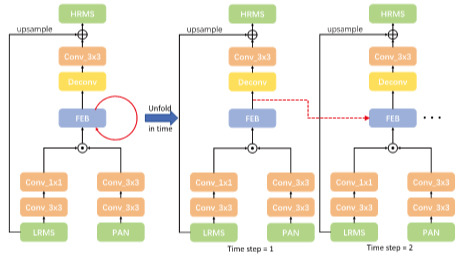
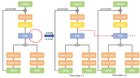
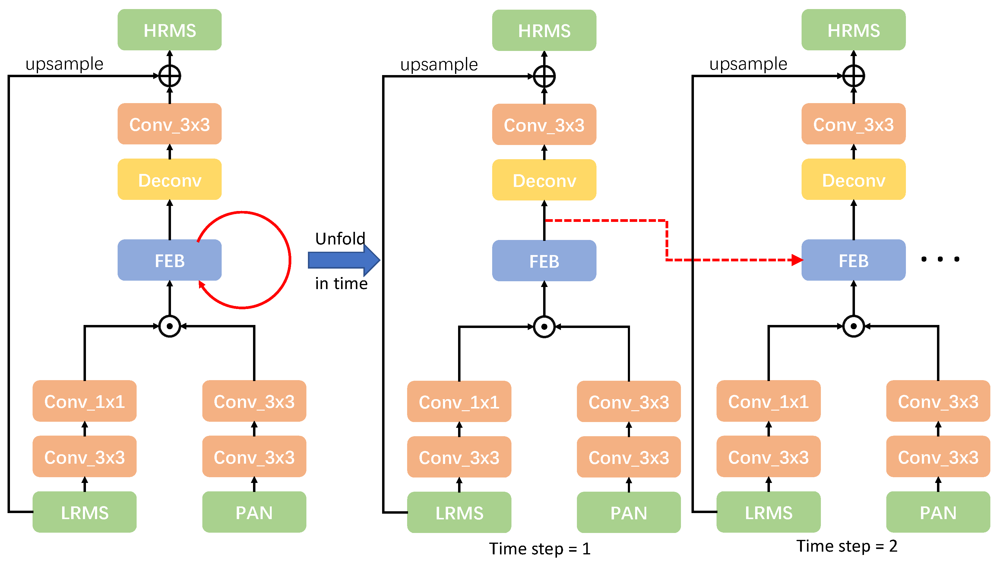
• We propose a two-path feedback network to extract features from the MS image and the PAN image separately and to achieve feedback mechanism which can carry powerful deep features to improve the poor shallow features in a feedback manner for better reconstruction performance.
• We attach losses to each time step to supervise the output of the network. In this way, the feedback deep features contain useful information, which comes from the coarsely-reconstructed HRMS at early time steps, to reconstruct better HRMS image at late time steps.

2. Materials

2.1. Datasets

To verify the effectiveness of we proposed method, we compare our proposed method with other pan-sharpening methods on five widely used datasets: Spot-6, Pléiades, IKONOS, QuickBird and WorldView-2.

Their characteristics are described in

Table 1. The spectral and spatial characteristic of PAN and MS iamges for five datasets.

			Spot-6	Pléiades	IKONOS	QuickBird	WorldView-2
Spectral Wavelength (nm)	PAN		455–745	470–830	450–900	450–900	450–800
	MS	Blue	455–525	430–550	400–520	450–520	450–510
		Green	530–590	500–620	520–610	520–600	510–580
		Red	625–695	590–710	630–690	630–690	630–690
		NIR(Near-infrared)	760–890	740–940	760–900	760–900	770–895
Spatial Resolution (m)	PAN		1.5	0.5	1.0	0.6	0.5
	MS		6.0	2.0	4.0	2.4	1.9

. Note that, for WorldView-2 dataset, The MS images have 8 bands which are named as Red, Green, Blue, Red Edge, Coastal, Yellow, near-infrared-1, near-infrared-2, respectively. To maintain consistency with the other datasets, Red, Green, Blue and near-infrared-1 band are used for evaluation in the experiments. As for our reference images in evaluation, we follow the Wald’s protocol [30]. We use bicubic interpolation to downsample the original MS and PAN images by a scale factor of 4 and feed the downsampled images into the network. We consider the original MS image as a reference.

2.2. Feedback Mechanism

The feedback mechanism commonly exists in the human visual system, which is able to carry information from high-level parts to low-level parts [31]. Lately, many works have made efforts to introduce feedback mechanism [26,27,29,32,33,34]. For single image super-resolution, Haris et al. [29] achieved iterative error feedback based on back-projection theory by up-projection and down-projection units. Han et al. [34] achieved delayed feedback mechanism by a dual-state RNN to transmit information between the two recurrent states.

The most relevant work to ours is [27], which elaborately designed a feedback block to extract powerful high-level representations for low-level computer vision tasks and transmitted the high-level representations to refine the low-level features. To introduce the feedback mechanism to pan-sharpening, we design a two-path pan-sharpening network with feedback connections (TPNwFB), which can process the PAN image and the MS image in two separate paths, and thus TPNwFB is a better choice for pan-sharpening.

3. Methods

In this part, the implementation details, the evaluation metrics, the network structure of the proposed TPNwFB and the loss function are described in detail.

3.1. Implementation Details

As suggested by Liu [5], we test our proposed network on the five datasets mentioned in Section 2.1, separately. We adopt the same data augmentation as [35] does. Following Wald’s protocol [30], there are 30,000 training samples for each dataset. We adopt PReLU [36] as our activation function attached after every convolutional layer and deconvolutional layer but the last layer in the network at each time step. We take the pan-sharpened image $I_{out}^T$, which is from the last time step as our pan-sharpened result. The proposed network is implemented by PyTorch [37] and trained on one NVIDIA RTX 2080Ti GPU. Adam optimizer [38] is employed to optimize the network with the initial learning rate 0.0001 and the momentum of 0.9. The mini-batch size is set to 4 and the size of image patches is set to $64\times 64$.

3.2. Evaluation Metrics

SAM [39], CC [5], $Q_4$ [40], RMSE [25], RASE [41] and ERGAS [42] are employed to quantitatively evaluate the pan-sharpening performance of our proposed method and contrastive methods.

• SAM. The spectral angle mapper (SAM) [39] evaluates the spectral distortions of the pan-sharpened image. It is defined as:

  $$SAM\left(x_1,x_2\right)=arccos\left(\frac{x_1·x_2}{∥x_1∥·∥x_2∥}\right),$$

  (1)

  where $x_1$ and $x_2$ are two spectral vectors.
• CC. The correlation coefficient (CC) [5] is used to evaluate the spectral quality of the pan-sharpened images. The CC is calculated by a pan-sharpened image I and the corresponding reference image Y.

  $$CC=\frac{Cov(I,Y)}{\sqrt{Var\left(I\right)Var\left(Y\right)}},$$

  (2)

  where $Cov(I,Y)$ is the covariance between I and Y, and $Var\left(n\right)$ denotes the variance of n.
• $Q_4$. The quality-index $Q_4$ [40] is the extension of the Q index [30]. $Q_4$ is defined as:

  $$Q_4=\frac{4\left|Cov(z_1,z_2)\right|·\left|Mean\left(z_1\right)\right|·\left|Mean\left(z_2\right)\right|}{(Va{r}^2\left(z_1\right)+Va{r}^2\left(z_2\right))(Mea{n}^2\left(z_1\right)+Mea{n}^2\left(z_2\right))},$$

  (3)

  where $z_1$ and $z_2$ are two quaternions formed by the spectral vectors of the MS image. $Cov(z_1,z_2)$ is the covariance between $z_1$ and $z_2$, $Var\left(n\right)$ denotes the variance of n, and $Mean\left(m\right)$ denotes the mean of m.
• RMSE. The root mean square error (RMSE) [25] is a frequently used measure of the differences between the pan-sharpened image I and the reference image Y.

  $$RMSE=\sqrt{\frac{1}{wh}\sum _{i=1}^w\sum _{j=1}^h{\left(Y_{i,j}-I_{i,j}\right)}^2},$$

  (4)

  where w and h are the width and height of the pan-sharpened image.
• RASE. The relative average spectral error (RASE) [41] estimates the global spectral quality of the pan-sharpened image. It is defined as:

  $$RASE=\frac{100}{M}\sqrt{\frac{1}{N}\sum _{i=1}^{N}RMSE{\left(B_i\right)}^2},$$

  (5)

  where $RMSE\left(B_i\right)$ is the root mean square error between the i-th band of the pan-sharpened image and the i-th band of the reference image. M is the mean value of the N spectral bands ($B_1,B_2\cdots ,B_N$).
• ERGAS. The relative global dimensional synthesis error (ERGAS) [42] is a commonly used index to measure the global quality. ERGAS is computed as the following expression:

  $$ERGAS=100\frac{h}{l}\sqrt{\frac{1}{N}\sum _{i=1}^N{\left(\frac{RMSE\left(B_i\right)}{Mean\left(B_i\right)}\right)}^2},$$

  (6)

  where h is the resolution of the pan-sharpened image, and l is the resolution of the low spatial resolution image. $RMSE\left(B_i\right)$ is the root mean square error between the i-th band of the pan-sharpened image and the i-th band of the reference image. $Mean\left(B_i\right)$ is the mean value of the i-th band of the low-resolution MS image. N is the number of the spectral bands.

3.3. Network Structure

To achieve feedback mechanism, we need to carry back useful deep features to refine the less powerful shallow features. Therefore, there are three necessary parts to achieve the feedback mechanism: (1) leveraging the recurrent structure to achieve iterative process. The iterative process allows powerful deep features to flow back to modify the poor low-level features. (2) providing the low-resolution MS image at each time step. This supplies the low-level features at each time step, which need improving. (3) attaching the loss to force the network reconstruct the HRMS image at each time step. This can ensure that the feedback features contains useful information from the coarsely-reconstructed HRMS image for reconstructing better HRMS image. As illustrated in the Figure 1, the proposed TPNwFB can be unfolded into T time steps. Time steps are placed in a chronological order for a clear illustration. To enforce the feedback information in TPNwFB to carry useful information for improving the low-level features, we attach the loss function to the output of the network at every time step. The discussion about the loss function for TPNwFB can be found in Section 3.5. The network at each time step t can be roughly divided into three parts: (1) two-path block (to extract features from the MS image and the PAN image separately), (2) feature extraction block (to generate powerful deep features through various upsampling-downsampling pairs and dense skip connections) and (3) reconstruction block (to reconstruct HRMS image). Note that the parameters are shared across all time steps to keep the network consistent. With the global skip connection at each time step, the network, at time step t, is to recover a residual image $I_{res}^t$, which is the difference between the HRMS image and the upsampled LRMS image. We denote a convolutional layer with kernel size $s\times s$ as $Con{v}_{s,n}(·)$, where n is the number of kernels. The output of a convolutional layer has the same spatial size with the input unless we say otherwise. Similarly, $Decon{v}_{s,n}(·)$ denotes a deconvolutional layer with n filters and kernel size $s\times s$.

The two-path block consists of two sub-networks to extract features from the MS image and the PAN image, respectively. The path that regards a four-band MS image as the input is denoted as “the MS path”. The other path that regards a single-band PAN image as the input is denoted as “the PAN path”. The MS path consists of one $Con{v}_{3,256}(·)$ layer and one $Con{v}_{1,64}(·)$ layer to extract features $F_{MS}$ from the MS image:

$$F_{MS}=Con{v}_{1,64}\left(Con{v}_{3,256}\left(I_{MS}\right)\right),$$

(7)

where $I_{MS}$ is the MS image. The PAN path contains two successive $Con{v}_{3,64}(·)$ layers with different parameters. The two convolutional layers in the PAN path have the stride of 2 to down-sampling the PAN image and extract features $F_{PAN}$ from the PAN image:

$$F_{PAN}=Con{v}_{3,64}\left(Con{v}_{3,64}\left(I_{PAN}\right)\right),$$

(8)

where $I_{PAN}$ is the PAN image. Finally, we concatenate $F_{MS}$ and $F_{PAN}$ to form the low-level features $F_i^t$ at time step t:

$$F_i^t=F_{MS}\odot F_{PAN},$$

(9)

where ⊙ refers to the concatenation operation. Then $F_i^t$ are used as the input of the following feature extraction block. Note that $F_i^1$ are considered as the initial feedback information $F_{fb}^0$.

The feature extraction block at t-th time step receives the feedback information $F_{fb}^{t-1}$ from the ($t-1$)-th time step and the low-level features $F_i^t$ from the t-th time step. $F_{fb}^t$ represents the feedback information, which is also the output of the feature extraction block at t-th time step. The output of the feature extraction block at t-th time step can be formulated as follows.

$$F_{fb}^t=f_{FEB}(F_{fb}^{t-1},F_i^t),$$

(10)

where $f_{FEB}(·,·)$ denotes the nested functions of the feature extraction block. The details of the feature extraction block are stated in Section 3.4.

The reconstruction part contains one $Decon{v}_{8,64}(·)$ layer with the stride of 4 and the padding of 2 and a $Con{v}_{3,4}(·)$ layer. The $Decon{v}_{8,64}(·)$ layer is used to upsample the low-resolution features with a scale factor $\times 4$. The $Con{v}_{3,4}(·)$ layer is to output the $I_{res}^t$. The function of the reconstruction part can be formulated as:

$$I_{res}^t=f_{re}\left(F_{fb}^t\right)=Con{v}_{3,4}\left(Decon{v}_{8,64}\left(F_{fb}^t\right)\right),$$

(11)

where $f_{re}(·)$ denotes the nested functions of the reconstruction part. Thus, the pan-sharpened image $I_{out}^t$, at time step t, can be obtained by:

$$I_{out}^t=I_{res}^t+f_{up}\left(I_{MS}\right),$$

(12)

where $f_{up}(·)$ is the upsampling operation to upsample the LRMS image with a scale factor $\times 4$. The choice of the upsampling kernel can be arbitrary. In this paper, we simply choose the bilinear upsampling kernel. After Ttime steps, we will totally obtain T pan-sharpened images $(I_{out}^1,I_{out}^2,\dots ,I_{out}^t,\dots I_{out}^T)$.

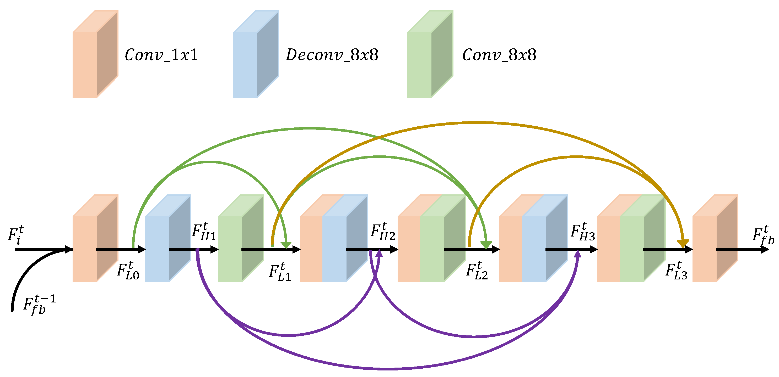
3.4. Feature Extraction Block

Figure 2 shows the feature extraction block (FEB). The FEB at the time step t receives the powerful deep features $F_{fb}^{t-1}$ from the ($t-1$)-th time step and the low-level features $F_i^t$ from the t-th time step. $F_{fb}^{t-1}$ are used to refine the low-level features $F_i^t$. Then, the feature extraction block generates more powerful deep features $F_{fb}^t$ which are passed to the reconstruction block and the next time step.

The FEB consists of G projection pairs with dense skip connections to link each pair. Each projection pair mainly has a deconvolutional layer to upsample the features and a convolutional layer to downsample the features. With multiple projection pairs, we iteratively up- and downsample the input features to achieve back-projection mechanism which enables the feature extraction block to generate more powerful features.

The feature extraction block at the t-th time step receives the low-level features $F_i^t$ and the feedback information $F_{fb}^{t-1}$. To refine the low-level features $F_i^t$ with the $F_{fb}^{t-1}$, we concatenate $F_i^t$ with $F_{fb}^{t-1}$ and use a $Con{v}_{1,64}(·)$ layer to compress the concatenated features, generating the refined low-level features $F_{L0}^t$:

$$F_{L0}^t=Con{v}_{1,64}(F_i^t\odot F_{fb}^{t-1}),$$

(13)

where ⊙ denotes the concatenation operation.

The upsampled features and the downsampled features produced by the g-th projection pair at the t-th time step are denoted as $F_{Hg}^t$ and $F_{Lg}^t$, respectively. $F_{Hg}^t$ can be obtained by:

$$F_{Hg}^t=Decon{v}_{8,64}(F_{L0}^t\odot F_{L1}^t\odot \cdots \odot F_{L(g-1)}^t),$$

(14)

where $Decon{v}_{8,64}(·)$ is a deconvolutional layer at the g-th projection pair with the kernel size of 8, the stride of 4 and the padding of 2. Correspondingly, $F_{Lg}^t$ can be obtained by:

$$F_{Lg}^t=Con{v}_{8,64}(F_{H1}^t\odot F_{H2}^t\odot \cdots \odot F_{Hg}^t),$$

(15)

where $Con{v}_{8,64}(·)$ is a convolutional layer at the g-th projection pair with the kernel size of 8, the stride of 4 and the padding of 2. Note that, except for the first projection pair, we add a $Con{v}_{1,64}$ layer before $Decon{v}_{8,64}(·)$ and $Con{v}_{8,64}(·)$ for feature fusion and computation efficiency.

To fully exploit the features produced by each projection pair and match the size of the input low-level features $F_i^{t+1}$ at the next time step, we use a $Con{v}_{1,64}(·)$ layer to fuse all the downsampled features produced by projection pairs to generate the output $F_{fb}^t$ of the feature extraction block at the t-th time step:

$$F_{fb}^t=Con{v}_{1,64}(F_{L1}^t\odot F_{L2}^t\odot \cdots \odot F_{LG}^t).$$

(16)

3.5. Loss Function

The network structure is an important factor affecting the quality of the pan-sharpened image, and the loss function is another important factor. Many of previous single image super-resolution and pan-sharpening methods take the $L_2$ loss function to optimize the parameters of the network [7,22,43,44]. However, the $L_2$ loss function may lead to unsatisfied artifacts at the flat areas due to that the $L_2$ loss function leads to a local minimum. In contrast, the $L_1$ loss function could obtain a better minimum. Besides, the $L_1$ loss function can preserve colors and luminance better than the $L_2$ loss function does [45]. Therefore, we choose the $L_1$ loss function to optimize the parameters of the proposed network. Since we have T time steps in one iteration and we attach the $L_1$ loss to the output of every time step, we totally have T pan-sharpened images $(I_{out}^1,I_{out}^2,\cdots ,I_{out}^T)$. T ground truth HRMS images $(I_{HRMS}^1,I_{HRMS}^2,\cdots ,I_{HRMS}^T)$ are paired with the T outputs in the proposed network. Note that $(I_{HRMS}^1,I_{HRMS}^2,\cdots ,I_{HRMS}^T)$ are the same with each other. The total loss function can be written as:

$$\mathcal{L}\left(\mathsf{\Theta }\right)=\frac{1}{MT}\sum _{t=1}^T{∥I_{HRMS}^t-I_{out}^t∥}_1,$$

(17)

where $\mathsf{\Theta }$ denotes the parameters in the network, and M denotes the samples numbers in each training batch.

4. Results

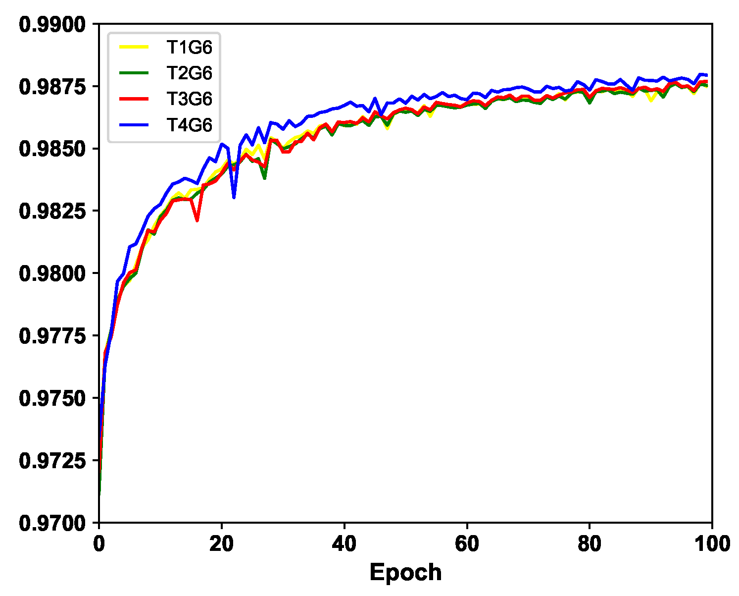
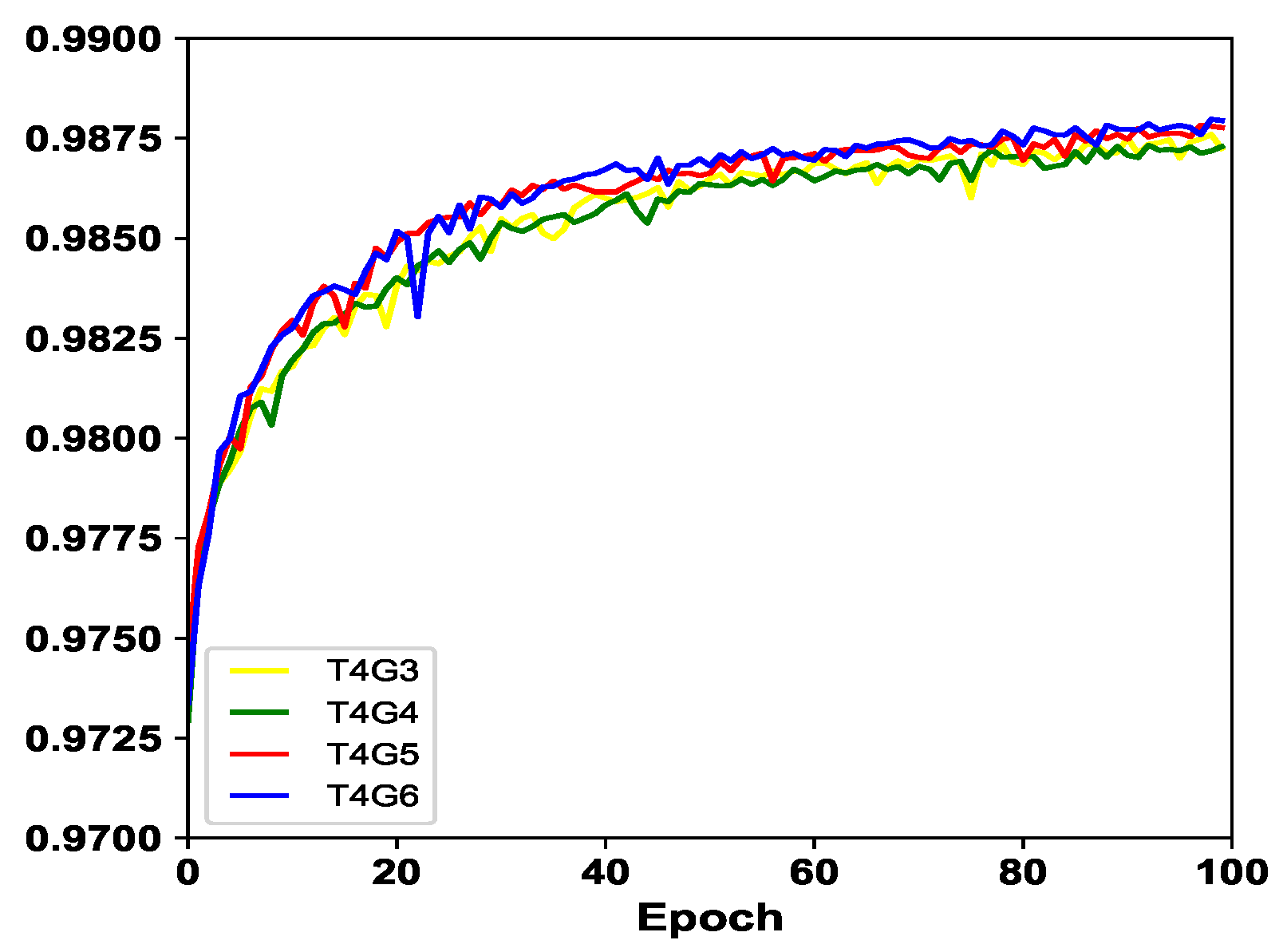
4.1. Impacts of G and T

We study the impacts of the number of time steps (denoted as T for short) and the number of projection pairs in the feature extraction block (denoted as G for short).

At first, we study the impact of T with G fixed. As shown in Figure 3, the network with feedback connection(s) can achieve improvement on pan-sharpening performance against the one without feedback (T = 1, the yellow line in Figure 3). Besides, it can be seen that the pan-sharpening performance can be further improved as T increases. Therefore, the network benefits from the feedback information across time steps.

Then, we investigate the impact of G with T fixed. Figure 4 shows that we can achieve better performance on pan-sharpening with larger value of G because of the stronger feature extraction ability of a deeper network. Therefore, larger T or G both can lead to more satisfying results. For simplicity, we choose T = 4 and G = 6 for analysis in the following subsections.

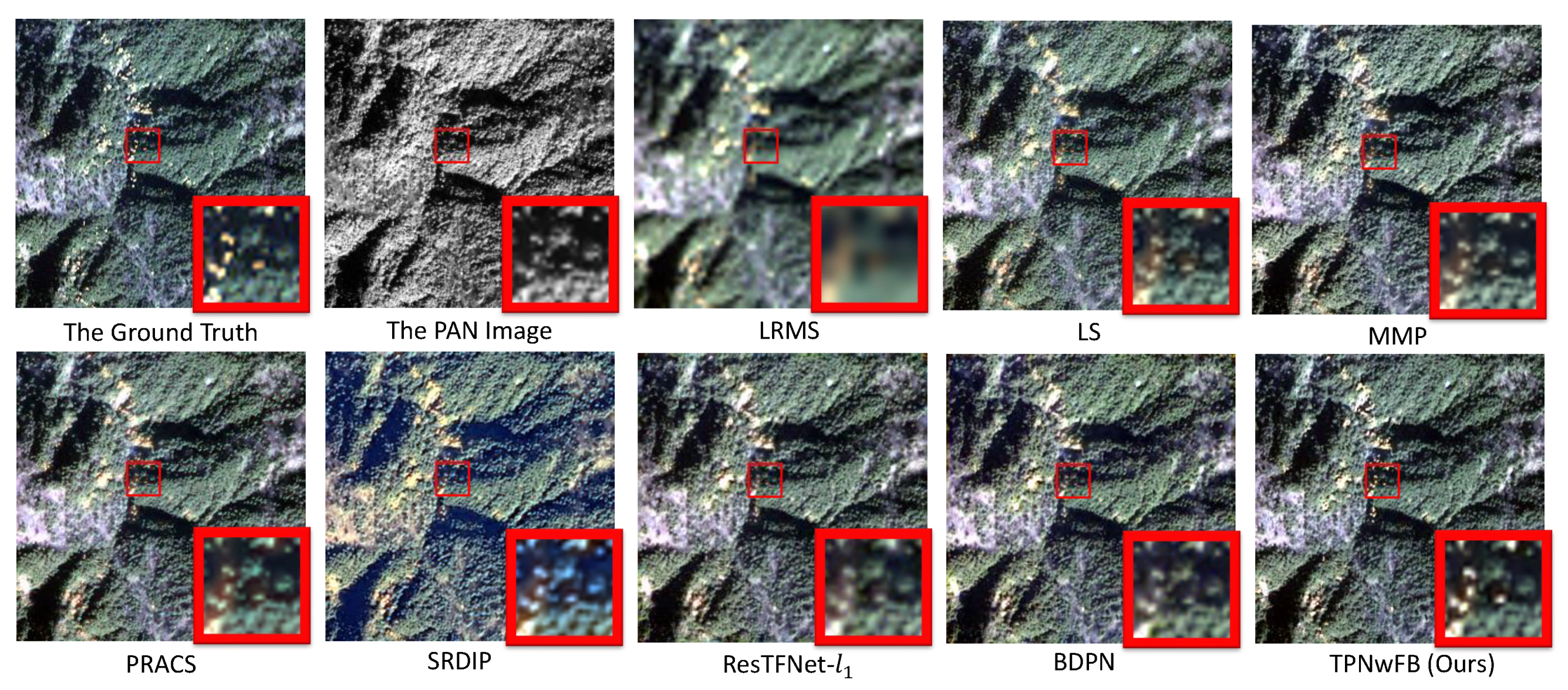
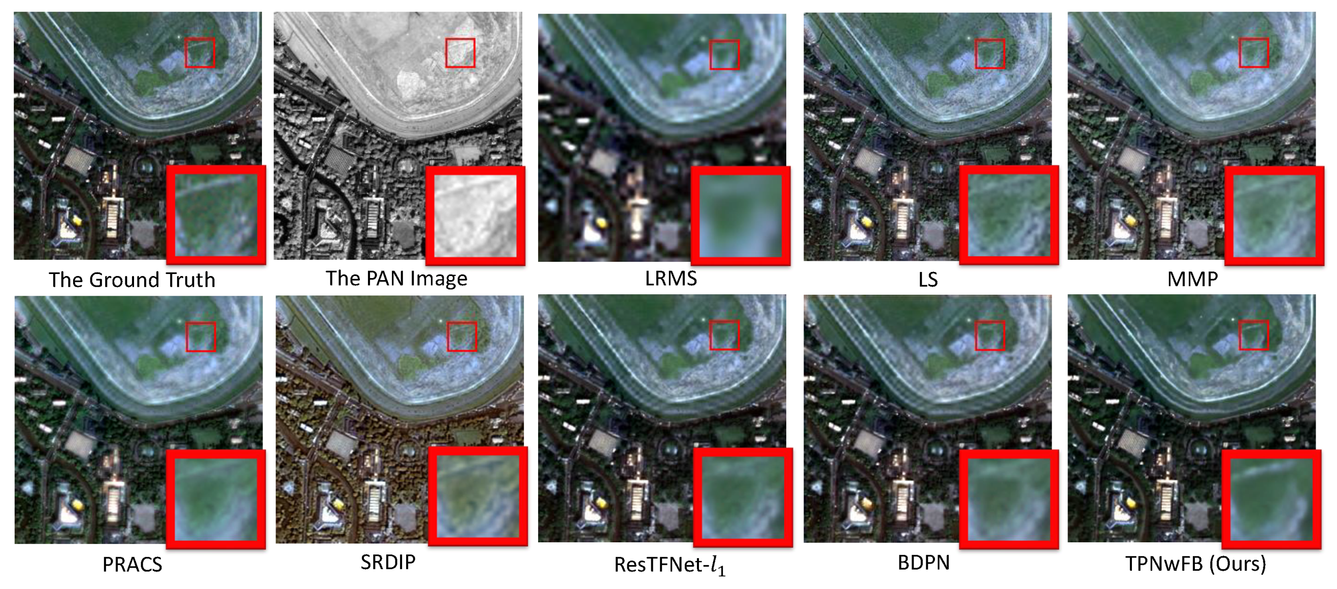
4.2. Comparisons with Other Methods

In this subsection, to evaluate the effectiveness of our proposed method, we compare TPNwFB with other six pan-sharpening methods: LS [46], MMP [47], PRACS [19], SRDIP [48], ResTFNet-$l_1$ [5], BDPN [25]. The objective results on the five datasets are reported in

Table 2. The objective results on Spot-6 dataset.

	CC↑	ERGAS↓	${\mathit{Q}}_4$↑	SAM↓	RASE↓	RMSE ↓
LS [46]	0.9239	3.4313	0.9230	0.0613	13.6192	38.6125
MMP [47]	0.9367	3.2491	0.9280	0.0610	13.1180	37.0925
PRACS [19]	0.9450	3.0492	0.9407	0.0634	12.3820	35.0980
SRDIP [48]	0.9488	2.7737	0.9414	0.0660	11.6139	32.8202
ResTFNet-$l_1$ [5]	0.9823	1.6693	0.9819	0.0443	7.1958	20.2944
BDPN [25]	0.9831	1.6320	0.9828	0.0436	7.0527	19.9081
TPNwFB	0.9880	1.3579	0.9879	0.0347	5.8065	16.3381

,

Table 3. The objective results on Pléiades dataset.

	CC↑	ERGAS↓	${\mathit{Q}}_4$↑	SAM↓	RASE↓	RMSE ↓
LS [46]	0.9518	3.2946	0.9515	0.0513	13.9496	84.43999
MMP [47]	0.9485	3.3855	0.9479	0.0568	14.3319	86.7706
PRACS [19]	0.9554	3.2297	0.9538	0.0563	13.8094	83.7290
SRDIP [48]	0.9541	3.0962	0.9518	0.0523	12.9734	78.4699
ResTFNet-$l_1$ [5]	0.9860	1.7609	0.9858	0.0360	7.4630	44.0964
BDPN [25]	0.9870	1.6828	0.9868	0.0386	7.1209	41.9430
TPNwFB	0.9952	0.9987	0.9952	0.0246	4.2994	25.4422

,

Table 4. The objective results on IKONOS dataset.

	CC↑	ERGAS↓	${\mathit{Q}}_4$↑	SAM↓	RASE↓	RMSE ↓
LS [46]	0.9177	3.1834	0.9139	0.0644	15.1032	34.5074
MMP [47]	0.9126	3.1986	0.9071	0.0626	14.8303	34.2762
PRACS [19]	0.9164	3.2966	0.9098	0.0682	16.0026	36.4808
SRDIP [48]	0.8896	3.4935	0.8743	0.0808	16.7381	37.2496
ResTFNet-$l_1$ [5]	0.9155	3.4025	0.9110	0.0693	15.7161	34.6267
BDPN [25]	0.9155	3.5082	0.9109	0.0690	15.8580	35.3906
TPNwFB	0.9612	2.0791	0.9602	0.0436	8.45813	18.4247

,

Table 5. The objective results on WorldView-2 dataset.

	CC↑	ERGAS↓	${\mathit{Q}}_4$↑	SAM↓	RASE↓	RMSE ↓
LS [46]	0.8989	5.4750	0.8953	0.0792	22.5279	65.7696
MMP [47]	0.8906	5.5598	0.8865	0.0798	22.8671	66.5725
PRACS [19]	0.8888	5.9043	0.8814	0.0832	24.9431	73.1840
SRDIP [48]	0.8940	5.4674	0.8880	0.0851	22.7510	66.4857
ResTFNet-$l_1$ [5]	0.9358	4.6079	0.9315	0.0646	18.3931	53.5033
BDPN [25]	0.9330	4.6347	0.9296	0.0725	18.8396	55.1684
TPNwFB	0.9817	2.3485	0.9813	0.0422	9.7115	28.7936

and

Table 6. The objective results of on QuickBird dataset.

	CC↑	ERGAS↓	${\mathit{Q}}_4$↑	SAM↓	RASE↓	RMSE ↓
LS [46]	0.9185	1.7127	0.9119	0.0395	6.8397	17.3581
MMP [47]	0.9181	1.7208	0.9001	0.0385	6.7145	17.0175
PRACS [19]	0.9031	1.7602	0.8852	0.0380	6.8669	17.4504
SRDIP [48]	0.8939	2.0369	0.8806	0.0544	8.3373	21.1365
ResTFNet-$l_1$ [5]	0.9500	1.3077	0.9474	0.0300	5.1326	13.0150
BDPN [25]	0.9445	1.3580	0.9418	0.0321	5.2913	13.4129
TPNwFB	0.9710	0.9643	0.9703	0.0221	3.7357	9.4888

, respectively. The pan-sharpening results of each dataset are obtained by averaging the results of all the test images. The best performance is shown in bold, and the second best performance is underlined.

From those tables, we can observe that the proposed TPNwFB can outperform the contrastive pan-sharpening methods by a large margin on all evaluation indexes. Besides, the proposed TPNwFB can constantly give the best results on all datasets while the performance of other pan-sharpening methods varies between datasets. This indicates the superiority of our proposed methods. On all datasets, the proposed TPNwFB provides the best CC and RMSE results, which indicates the pan-sharpened image produced by TPNwFB is the closest to the reference image. That is to say we have successfully enhanced the spatial resolution. Moreover, with the best results on SAM and RASE, TPNwFB can keep good spectral quality after pan-sharpening. From the point of global quality (ERGAS and $Q_4$), TPNwFB also achieves the best performance.

We also provide some subjective results, as shown in Figure 5, Figure 6 and Figure 7. From Figure 5, we can see that our proposed method gives more clearer details and sharper edges, which is crucial for accurately monitoring. In Figure 6, our proposed method does not introduce color distortion and bring fewer artifacts. The pan-sharpened image produced by TPNwFB presents the most clear outline of the building compared with other pan-sharpening methods. In Figure 7, our proposed method presents the most clear white line without color distortion. The aforementioned comparisons demonstrate the effectiveness and robustness of our proposed TPNwFB.

5. Discussions

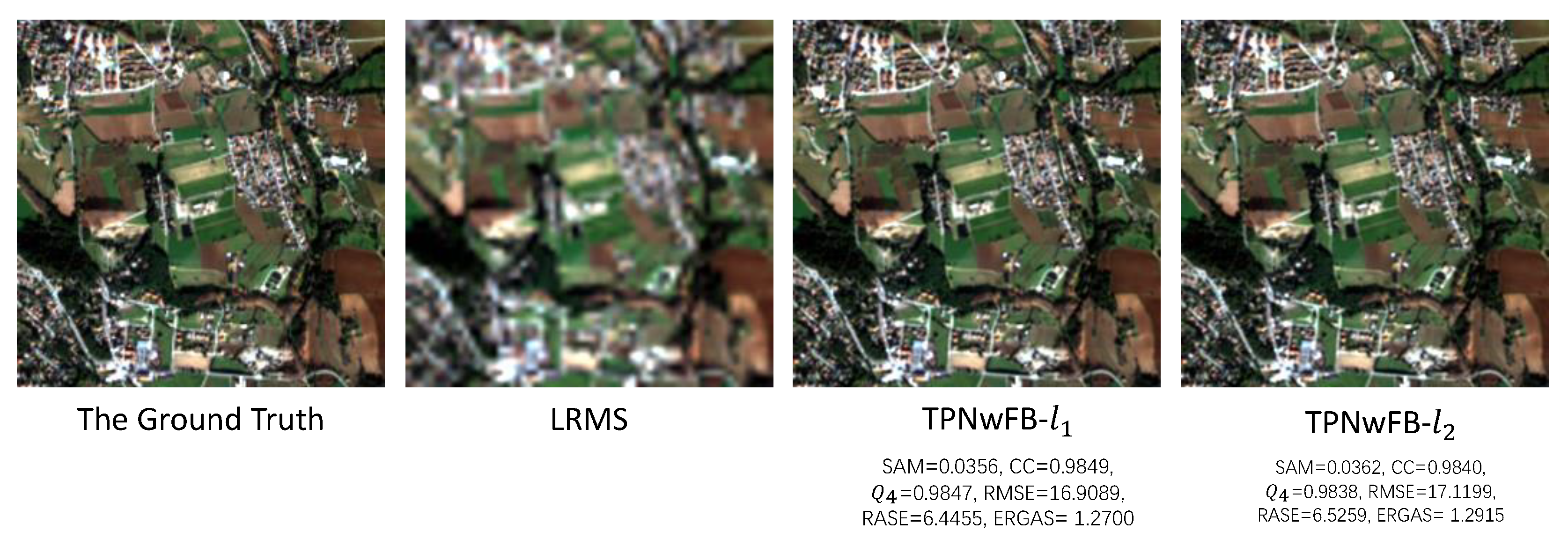
5.1. Discussions on Loss Functions

In this subsection, we compare the TPNwFB trained with $l_1$ loss function (denoted as TPNwFB-$l_1$ for short) with the TPNwFB trained with $l_2$ loss function (denoted as TPNwFB-$l_2$ for short). The subjective and objective results are shown in Figure 8. It can be seen the pan-sharpened image generated by TPNwFB-$l_1$ gives more clear details and sharper edges around water bodies when compared with the ones produced by TPNwFB-$l_2$. The objective results also suggest that the spatial and spectral quality of the pan-sharpened image can be improved by the $l_1$ loss function. We choose $l_1$ loss function as our default loss function for analysis in the following experiments.

5.2. Discussions on Feedback Mechanism

To investigate the feedback mechanism in the proposed network, we trained a feedforward one, which is the counterpart of the TPNwFB. By disconnecting the loss from the 1st time step to the ($T-1$)-th time step (the loss attached to the final T-th step is kept), the network is impossible to refine the low-level features with the useful information which carries a notion of the pan-sharpened image. Therefore, the feedback network TPNwFB degrades to its feedforward counterpart, which is denoted as TPN-FF. The TPN-FF still keeps the recurrent structure and can output four intermediate pan-sharpened images. Note that these four pan-sharpened images have no loss to supervise the performance. We then compare the SAM, CC and $Q_4$ values of all intermediate pan-sharpened images from TPNwFB and TPN-FF. The results are shown in

Table 7. The impacts of feedback mechanism on Spot-6 dataset.

	SAM↓				CC↑				${\mathit{Q}}_4\uparrow$
Time step	1st	2nd	3rd	4th	1st	2nd	3rd	4th	1st	2nd	3rd	4th
TPNwFB	0.0321	0.0319	0.0319	0.0319	0.9875	0.9875	0.9876	0.9876	0.9874	0.9874	0.9875	0.9875
TPN-FF	0.0427	0.0335	0.0326	0.0320	0.9776	0.9862	0.9871	0.9874	0.9769	0.9859	0.9871	0.9873

.

From Table 7, we have two observations. The first observation is that the feedback network TPNwFB outperforms TPN-FF at every time step. This indicates the proposed TPNwFB actually can benefit from the feedback connections instead of the recurrent network structure because both networks keep the recurrent structures. Another observation is that the proposed TPNwFB shows high pan-sharpening quality at early time steps due to the feedback mechanism.

To show how the feedback mechanism impacts the pan-sharpening performance, we visualize the output of the feature extraction block at each time step in TPNwFB and TPN-FF, as shown in Figure 9. The visualizations are the channel-wise mean of $F_{fb}^t$, which can represent the output of the feature extraction part at the time step t.

With the global residual connections, we aim at recovering the residual image to predict high frequency components. From Figure 9, we can see that the feedback network TPNwFB can produce feature maps $F_{fb}^t$ with more negative values compared with TPN-FF, showing powerful ability to suppress the smooth areas. This further leads to more high frequency components. Besides, the features produced by TPN-FF vary significantly from the first time step to the last time step: edges are outlined at early time steps and smooth areas are suppressed at late time steps. On the other hand, with feedback connections, the proposed TPNwFB can take a self-correcting process since it can obtain well-developed feature maps at early time steps. This different pattern indicates that TPNwFB can reroute deep features to refine shallow features. Consequently, the shallow layers can develop better representations at late time steps, improving the pan-sharpening performance.

6. Conclusions

In this paper, we propose a two-path network with feedback connections for pan-sharpening (TPNwFB). In the proposed TPNwFB, the PAN and the LRMS images are processed separately to make full use of both images. Besides, the powerful deep features, which contain useful information from coarsely reconstructed HRMS at early time steps, are carried back through feedback connections to refine the low-level features. The loss function is attached to every time step to ensure the feedback information contains a notion of the pan-sharpened image. Furthermore, the special feature extraction block is used to extract powerful deep features and to effectively handle the feedback information. With feedback connections, the proposed TPNwFB can take a self-correcting process since it can obtain well-developed feature maps ta early time steps. Extensive experiments have demonstrated the effectiveness of our proposed method on pan-sharpening.

References

1. Ghassemian, H. A review of remote sensing image fusion methods. Inf. Fusion 2016, 32, 75–89. [Google Scholar] [CrossRef]
2. Nikolakopoulos, K.G. Comparison of nine fusion techniques for very high resolution data. Photogramm. Eng. Remote Sens. 2008, 74, 647–659. [Google Scholar] [CrossRef] [Green Version]
3. Pohl, C.; Van Genderen, J.L. Review article multisensor image fusion in remote sensing: Concepts, methods and applications. Int. J. Remote Sens. 1998, 19, 823–854. [Google Scholar] [CrossRef] [Green Version]
4. Vivone, G.; Alparone, L.; Chanussot, J.; Dalla Mura, M.; Garzelli, A.; Licciardi, G.A.; Restaino, R.; Wald, L. A critical comparison among pansharpening algorithms. IEEE Trans. Geosci. Remote Sens. 2014, 53, 2565–2586. [Google Scholar] [CrossRef]
5. Liu, X.; Liu, Q.; Wang, Y. Remote sensing image fusion based on two-stream fusion network. Inf. Fusion 2020, 55, 1–15. [Google Scholar] [CrossRef] [Green Version]
6. Wei, Y.; Yuan, Q.; Shen, H.; Zhang, L. Boosting the accuracy of multispectral image pansharpening by learning a deep residual network. IEEE Geosci. Remote Sens. Lett. 2017, 14, 1795–1799. [Google Scholar] [CrossRef] [Green Version]
7. Masi, G.; Cozzolino, D.; Verdoliva, L.; Scarpa, G. Pansharpening by convolutional neural networks. Remote Sens. 2016, 8, 594. [Google Scholar] [CrossRef] [Green Version]
8. Tu, T.M.; Su, S.C.; Shyu, H.C.; Huang, P.S. A new look at IHS-like image fusion methods. Inf. Fusion 2001, 2, 177–186. [Google Scholar] [CrossRef]
9. Tu, T.M.; Huang, P.S.; Hung, C.L.; Chang, C.P. A fast intensity-hue-saturation fusion technique with spectral adjustment for IKONOS imagery. IEEE Geosci. Remote Sens. Lett. 2004, 1, 309–312. [Google Scholar] [CrossRef]
10. Shahdoosti, H.R.; Ghassemian, H. Combining the spectral PCA and spatial PCA fusion methods by an optimal filter. Inf. Fusion 2016, 27, 150–160. [Google Scholar] [CrossRef]
11. Xu, Q.; Li, B.; Zhang, Y.; Ding, L. High-fidelity component substitution pansharpening by the fitting of substitution data. IEEE Trans. Geosci. Remote Sens. 2014, 52, 7380–7392. [Google Scholar]
12. Parente, C.; Santamaria, R. Increasing geometric resolution of data supplied by quickbird multispectral sensors. Sens. Transducers 2013, 156, 111. [Google Scholar]
13. Pradhan, P.S.; King, R.L.; Younan, N.H.; Holcomb, D.W. Estimation of the number of decomposition levels for a wavelet-based multiresolution multisensor image fusion. IEEE Trans. Geosci. Remote Sens. 2006, 44, 3674–3686. [Google Scholar] [CrossRef]
14. Nunez, J.; Otazu, X.; Fors, O.; Prades, A.; Pala, V.; Arbiol, R. Multiresolution-based image fusion with additive wavelet decomposition. IEEE Trans. Geosci. Remote Sens. 1999, 37, 1204–1211. [Google Scholar] [CrossRef] [Green Version]
15. Nencini, F.; Garzelli, A.; Baronti, S.; Alparone, L. Remote sensing image fusion using the curvelet transform. Inf. Fusion 2007, 8, 143–156. [Google Scholar] [CrossRef]
16. Fang, F.; Li, F.; Shen, C.; Zhang, G. A variational approach for pan-sharpening. IEEE Trans. Image Process. 2013, 22, 2822–2834. [Google Scholar] [CrossRef]
17. Jiang, C.; Zhang, H.; Shen, H.; Zhang, L. Two-step sparse coding for the pan-sharpening of remote sensing images. IEEE J. Sel. Top. Appl. Earth Obs. Remote Sens. 2013, 7, 1792–1805. [Google Scholar] [CrossRef]
18. Padwick, C.; Deskevich, M.; Pacifici, F.; Smallwood, S. WorldView-2 pan-sharpening. In Proceedings of the ASPRS 2010 Annual Conference, San Diego, CA, USA, 26–30 April 2010; Volume 2630. [Google Scholar]
19. Choi, J.; Yu, K.; Kim, Y. A new adaptive component-substitution-based satellite image fusion by using partial replacement. IEEE Trans. Geosci. Remote Sens. 2010, 49, 295–309. [Google Scholar] [CrossRef]
20. Hussain, S.; Keung, J.; Khan, A.A.; Ahmad, A.; Cuomo, S.; Piccialli, F.; Jeon, G.; Akhunzada, A. Implications of deep learning for the automation of design patterns organization. J. Parallel Distrib. Comput. 2018, 117, 256–266. [Google Scholar] [CrossRef]
21. Ahmed, I.; Ahmad, A.; Piccialli, F.; Sangaiah, A.K.; Jeon, G. A robust features-based person tracker for overhead views in industrial environment. IEEE Internet Things J. 2017, 5, 1598–1605. [Google Scholar] [CrossRef]
22. Dong, C.; Loy, C.C.; He, K.; Tang, X. Learning a deep convolutional network for image super-resolution. In European Conference on Computer Vision, Zurich, Switzerland, 6–12 September 2014; Springer: Berlin, Germany, 2014; pp. 184–199. [Google Scholar]
23. Jeon, G.; Anisetti, M.; Wang, L.; Damiani, E. Locally estimated heterogeneity property and its fuzzy filter application for deinterlacing. Inf. Sci. 2016, 354, 112–130. [Google Scholar] [CrossRef]
24. Zhong, J.; Yang, B.; Huang, G.; Zhong, F.; Chen, Z. Remote sensing image fusion with convolutional neural network. Sens. Imaging 2016, 17, 10. [Google Scholar] [CrossRef]
25. Zhang, Y.; Liu, C.; Sun, M.; Ou, Y. Pan-Sharpening Using an Efficient Bidirectional Pyramid Network. IEEE Trans. Geosci. Remote Sens. 2019, 57, 5549–5563. [Google Scholar] [CrossRef]
26. Zamir, A.R.; Wu, T.L.; Sun, L.; Shen, W.B.; Shi, B.E.; Malik, J.; Savarese, S. Feedback networks. In Proceedings of the IEEE Conference on Computer Vision and Pattern Recognition, Honolulu, HI, USA, 21–26 July 2017; pp. 1308–1317. [Google Scholar]
27. Li, Z.; Yang, J.; Liu, Z.; Yang, X.; Jeon, G.; Wu, W. Feedback Network for Image Super-Resolution. In Proceedings of the IEEE Conference on Computer Vision and Pattern Recognition, Long Beach, CA, USA, 15–20 June 2019; pp. 3867–3876. [Google Scholar]
28. Timofte, R.; Rothe, R.; Van Gool, L. Seven ways to improve example-based single image super resolution. In Proceedings of the IEEE Conference on Computer Vision and Pattern Recognition, Las Vegas, NV, USA, 27–30 June 2016; pp. 1865–1873. [Google Scholar]
29. Haris, M.; Shakhnarovich, G.; Ukita, N. Deep back-projection networks for super-resolution. In Proceedings of the IEEE Conference on Computer Vision and Pattern Recognition, Munich, Germany, 8–14 September 2018; pp. 1664–1673. [Google Scholar]
30. Wald, L.; Ranchin, T.; Mangolini, M. Fusion of Satellite Images of Different Spatial Resolutions: Assessing the Quality of Resulting Images. Photogramm. Eng. Remote Sens. 1997, 63, 691–699. [Google Scholar]
31. Hupé, J.; James, A.; Payne, B.; Lomber, S.; Girard, P.; Bullier, J. Cortical feedback improves discrimination between figure and background by V1, V2 and V3 neurons. Nature 1998, 394, 784. [Google Scholar] [CrossRef] [PubMed]
32. Carreira, J.; Agrawal, P.; Fragkiadaki, K.; Malik, J. Human pose estimation with iterative error feedback. In Proceedings of the IEEE Conference on Computer Vision and Pattern Recognition, Las Vegas, NV, USA, 26 June–1 July 2016; pp. 4733–4742. [Google Scholar]
33. Cao, C.; Liu, X.; Yang, Y.; Yu, Y.; Wang, J.; Wang, Z.; Huang, Y.; Wang, L.; Huang, C.; Xu, W.; et al. Look and think twice: Capturing top-down visual attention with feedback convolutional neural networks. In Proceedings of the IEEE International Conference on Computer Vision, Santiago, Chile, 7–13 December 2015; pp. 2956–2964. [Google Scholar]
34. Han, W.; Chang, S.; Liu, D.; Yu, M.; Witbrock, M.; Huang, T.S. Image super-resolution via dual-state recurrent networks. In Proceedings of the IEEE Conference on Computer Vision and Pattern Recognition, Long Beach, CA, USA, 8 September 2018; pp. 1654–1663. [Google Scholar]
35. Lim, B.; Son, S.; Kim, H.; Nah, S.; Mu Lee, K. Enhanced deep residual networks for single image super-resolution. In Proceedings of the IEEE Conference on Computer Vision and Pattern Recognition Workshops, Honolulu, HI, USA, 21–26 July 2017; pp. 136–144. [Google Scholar]
36. He, K.; Zhang, X.; Ren, S.; Sun, J. Delving deep into rectifiers: Surpassing human-level performance on imagenet classification. In Proceedings of the IEEE International Conference on Computer Vision, Santiago, Chile, 7–13 December 2015; pp. 1026–1034. [Google Scholar]
37. Paszke, A.; Gross, S.; Massa, F.; Lerer, A.; Bradbury, J.; Chanan, G.; Killeen, T.; Lin, Z.; Gimelshein, N.; Antiga, L.; et al. PyTorch: An Imperative Style, High-Performance Deep Learning Library. In Advances in Neural Information Processing Systems. 2019, pp. 8024–8035. Available online: http://papers.nips.cc/paper/9015-pytorch-an-imperative-style-high-performance-deep-learning-library (accessed on 13 April 2020).
38. Kingma, D.P.; Ba, J. Adam: A method for stochastic optimization. arXiv 2014, arXiv:1412.6980. [Google Scholar]
39. Yuhas, R.H.; Goetz, A.F.; Boardman, J.W. Discrimination among semi-arid landscape endmembers using the spectral angle mapper (SAM) algorithm. In Proceedings of the Summaries 3rd Annual JPL Airborne Geoscience Workshop, Pasadena, CA, USA, 1–5 June 1992; pp. 147–149. [Google Scholar]
40. Alparone, L.; Baronti, S.; Garzelli, A.; Nencini, F. A global quality measurement of pan-sharpened multispectral imagery. IEEE Geosci. Remote Sens. Lett. 2004, 1, 313–317. [Google Scholar] [CrossRef]
41. Pushparaj, J.; Hegde, A.V. Evaluation of pan-sharpening methods for spatial and spectral quality. Appl. Geomat. 2017, 9, 1–12. [Google Scholar] [CrossRef]
42. Wald, L. Quality of high resolution synthesised images: Is there a simple criterion? In Proceedings of the Fusion of Earth Data: Merging Point Measurements, Raster Maps, and Remotely Sensed Image, Nice, France, 26–28 January 2000. [Google Scholar]
43. Yang, J.; Fu, X.; Hu, Y.; Huang, Y.; Ding, X.; Paisley, J. PanNet: A deep network architecture for pan-sharpening. In Proceedings of the IEEE International Conference on Computer Vision, Venice, Italy, 22–29 October 2017; pp. 5449–5457. [Google Scholar]
44. Kim, J.; Kwon Lee, J.; Mu Lee, K. Accurate image super-resolution using very deep convolutional networks. In Proceedings of the IEEE Conference on Computer Vision and Pattern Recognition, Las Vegas, NV, USA, 26 June–1 July 2016; pp. 1646–1654. [Google Scholar]
45. Zhao, H.; Gallo, O.; Frosio, I.; Kautz, J. Loss functions for image restoration with neural networks. IEEE Trans. Comput. Imaging 2016, 3, 47–57. [Google Scholar] [CrossRef]
46. Jin, B.; Kim, G.; Cho, N.I. Wavelet-domain satellite image fusion based on a generalized fusion equation. J. Appl. Remote Sens. 2014, 8, 080599. [Google Scholar] [CrossRef] [Green Version]
47. Kang, X.; Li, S.; Benediktsson, J.A. Pansharpening with matting model. IEEE Trans. Geosci. Remote Sens. 2013, 52, 5088–5099. [Google Scholar] [CrossRef]
48. Yin, H. Sparse representation based pansharpening with details injection model. Signal Proc. 2015, 113, 218–227. [Google Scholar] [CrossRef]
Figure 1. The architecture of our proposed TPNwFB. The red arrows denote the feedback connections. ⊙ denotes concatenating the features from the LRMS image and the features from the PAN image. ⊕ denotes element-wise addition. Conv_ s × s denotes the convolutional layer with kernel size s × s .
Remotesensing 12 01674 g001
Figure 2. The diagram of the feature extraction block. The D e c o n v _ 8 × 8 denotes the deconvolutional layer with kernel_size = 8, stride = 4 and padding = 2. The C o n v _ 8 × 8 denotes the convolutional layer with kernel_size = 8, stride = 4 and padding = 2. The C o n v _ 1 × 1 denotes the convolutional layer with kernel_size = 1, stride = 1 and padding = 0. The figure gives the example of 3 projection pairs.
Remotesensing 12 01674 g002
Figure 3. The analysis of T with G fixed to 6. The figure gives the CC values on Spot-6 dataset.
Remotesensing 12 01674 g003
Figure 4. The analysis of G with T fixed to 4. The figure gives the CC values on Spot-6 dataset.
Remotesensing 12 01674 g004
Figure 5. Visual results of different pan-sharpening methods on the IKONOS dataset.
Remotesensing 12 01674 g005
Figure 6. Visual results of different pan-sharpening methods on the WorldView-2 dataset.
Remotesensing 12 01674 g006
Figure 7. Visual results of different pan-sharpening methods on the QuickBird dataset.
Remotesensing 12 01674 g007
Figure 8. Comparisons of TPNwFB networks trained with different loss functions.
Remotesensing 12 01674 g008
Figure 9. The visualizations of F f b t at each time step in TPN-FF and TPNwFB.
Remotesensing 12 01674 g009