Accuracies of Soil Moisture Estimations Using a Semi-Empirical Model over Bare Soil Agricultural Croplands from Sentinel-1 SAR Data

Abstract

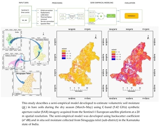
This study describes a semi-empirical model developed to estimate volumetric soil moisture (${\vartheta }_v$) in bare soils during the dry season (March–May) using C-band (5.42 GHz) synthetic aperture radar (SAR) imagery acquired from the Sentinel-1 European satellite platform at a 20 m spatial resolution. The semi-empirical model was developed using backscatter coefficient ($\mathsf{\sigma }°\mathrm{dB}$) and in situ soil moisture collected from Siruguppa taluk (sub-district) in the Karnataka state of India. The backscatter coefficients ${\sigma }_{VV}^0$ and ${\sigma }_{VH}^0$ were extracted from SAR images at 62 geo-referenced locations where ground sampling and volumetric soil moisture were measured at a 10 cm (0–10 cm) depth using a soil core sampler and a standard gravimetric method during the dry months (March–May) of 2017 and 2018. A linear equation was proposed by combining ${\sigma }_{VV}^0$ and ${\sigma }_{VH}^0$ to estimate soil moisture. Both localized and generalized linear models were derived. Thirty-nine localized linear models were obtained using the 13 Sentinel-1 images used in this study, considering each polarimetric channel Co-Polarization (VV) and Cross-Polarization (VH) separately, and also their linear combination of VV + VH. Furthermore, nine generalized linear models were derived using all the Sentinel-1 images acquired in 2017 and 2018; three generalized models were derived by combining the two years (2017 and 2018) for each polarimetric channel; and three more models were derived for the linear combination of ${\sigma }_{VV}^0$ and ${\sigma }_{VH}^0$. The above set of equations were validated and the Root Mean Square Error (RMSE) was 0.030 and 0.030 for 2017 and 2018, respectively, and 0.02 for the combined years of 2017 and 2018. Both localized and generalized models were compared with in situ data. Both kind of models revealed that the linear combination of ${\sigma }_{VV}^0$ + ${\sigma }_{VH}^0$ showed a significantly higher R² than the individual polarimetric channels.

1. Introduction

Soil moisture estimation across space and time has become possible with the advent of microwave remote sensing [1]. The amount of moisture in the soil is a function of physical, chemical, and management practices. Soil moisture is highly dynamic across space and correlated in time. The radar backscattering coefficient is a function of soil characteristics such as dielectric constant, texture, and surface roughness, and depends on the wavelength, polarization, and angle of incidence of the radar [1]. Shorter wavelength C-band radar backscatter has shown sensitivity to surface soil moisture at a depth of about 5 cm [2,3,4]. The launch of the Sentinel-1 mission of the European Space Agency has made a huge amount of C-band data acquired since 2014 from all over the Earth’s surface accessible. This opened up new perspectives on studying soil moisture in semi-arid regions, as was undertaken in Karnataka, India, in this work. Large scale soil moisture monitoring will provide greater insights into energy fluxes, which can result in improved meteorological and climatic projections [5] that will provide critical inputs for agriculture.

There have been studies based on physical, empirical, and semi-empirical models that estimate soil moisture over bare soils through radar remote sensing [6,7,8]. Physical approaches require many input parameters such as surface roughness and slope, which are not available under practical conditions [8]. Empirical models are only data driven, whereas semi-empirical models, while being data driven, also support theoretical considerations. In soil studies, they are site-specific and generally valid for specific soil characteristics [3]. Previous semi-empirical studies have considered single polarization to build a relationship between soil moisture and a backscatter model at 10 cm depth [9] and estimated ${\vartheta }_v$ with a root mean square error (RMSE) of 3–6% [10,11,12] using C-band data. There have also been studies that have used the SAR interferometry technique and Sentinel-1 data to estimate soil moisture and compare them with in situ measurements [13]. Even though SAR interferometry is less frequently used in the remote sensing community to estimate soil moisture, its advantage lies in its ability to disentangle moisture and terrain roughness contributions. Most SAR-based soil moisture estimation studies have covered small areas limited to a few hundred square kilometers [11,12,13,14,15,16,17]. Estimating soil moisture over a wider area and at a higher resolution using SAR imagery will provide information on managing water resources and irrigation scheduling that can benefit a large number of farmers [14].

The aim of this study was to estimate soil moisture in bare rice agricultural soils. While SAR images have been used to estimate rice phenology using X-band TerraSAR-X images [15], there have been limited studies to estimate the soil moisture in bare rice agricultural soils using Sentinel-1 C-band images. Bare soils in Siruguppa are rice growing areas that lie bare after the rice crop has been harvested in March, with rice stubble and weeds that have dried up during summer (March–June). By the time the monsoon rains start, it is extremely critical to estimate the amount of soil moisture in the top 10 cm, which will help farmers decide when to start preparing the land and start sowing the next crop. Surface roughness, soil status, soil moisture, and crop residue distribution affect radar backscatter [16]. It is well established that ${\sigma }_{VV}^0$ is more sensitive to variation in soils and ${\sigma }_{VH}^0$ is more suited to the identification of dry crop residue [17]. Utilizing both together can improve the accuracy of soil moisture estimates [18]. Nevertheless, soil moisture studies using ${\sigma }_{VV}^0$ and ${\sigma }_{VH}^0$ together, especially using Sentinel 1 SAR data, are limited. The need for such studies over significantly large agricultural fields is very important to study agriculture, water, and food security. The major goal of this study was to estimate soil moisture over bare soils using both ${\sigma }_{VV}^0$ and ${\sigma }_{VH}^0$ polarization and compare it with in situ measurements at a 10 cm (0–10 cm) depth. At the time of measurement, soil moisture to 10 cm is at the steady state and consistent across that top surface layer and therefore the C-band can be assumed to detect the top 10 cm layer. However, it is known that C-band SAR signals cannot penetrate to a 10 cm depth.

The contribution of standing stubble to total backscattering coefficient is comparable with that of the soil surface when the stubble has more than 75% water content. Backscatter coefficient decreases with a decrease in water content in the stubble. However, when the water content in the stubble is less than 40%, the contribution to the total backscattering coefficient is negligible [19]. We investigated both localized and generalized linear models to try to disentangle the stubble and soil moisture contributions. The linear coefficients of localized models were derived using in situ data acquired on a specific Sentinel-1 day. In contrast, generalized models were built using all in situ measurements acquired in the study period, thus adding the temporal dimension to the analysis of Sentinel-1 data. The question we wanted to answer is: can semi-empirical models estimate soil moisture, getting rid of the stubble contribution to the backscattering coefficient? We tried to answer this question by studying the effects of each variable, time, and polarization, separately. A localized model does not take into account the temporal evolution of backscattering, while a generalized model includes the time variable when estimating the linear coefficients. Furthermore, for each model, it is possible to keep the polarimetric channels separated or merge them. In this work, we used a large dataset of in situ measurements of soil-moisture acquired across a 2-year period to answer the above question. The issues of the stability of results and of collinearity of data are crucial and will be used to assess the results of this experiment.

The rest of this paper is organized as follows: Section 2 is devoted to materials and methods, Section 3 to the results, and Section 4 presents the discussion. Finally, a few conclusions are drawn in Section 5.

2. Materials and Methods

2.1. Study Area

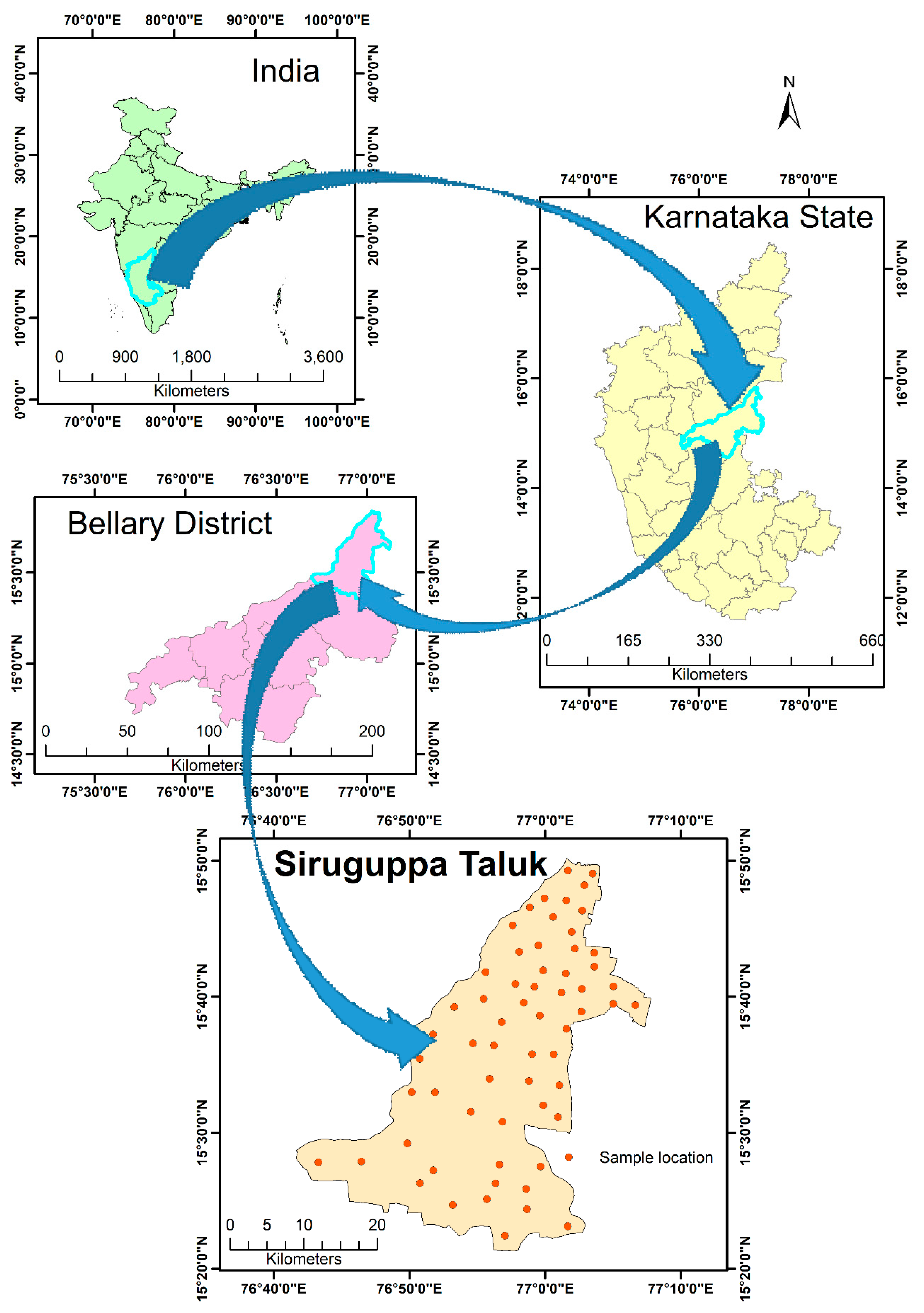
The study was conducted in Siruguppa taluk (sub-district) in the Bellary district of Karnataka state, India (Figure 1). Siruguppa is located between 15.35°N to 15.83°N latitudes and 76.69°E to 76.71°E longitudes covering an area of 1048 sq. km. Its climate is moderate and dry most of the year. It experiences high temperatures ranging from 23.2 °C to 42.4 °C from March to May and an annual rainfall of 645 mm. Irrigation from canal discharges cater to 60% of the cropped area, and the rest is either rainfed or irrigated through groundwater. Most of the crops are grown in predominantly black-clay, red-loamy, and red-sandy soils.

The River Tungabhadra runs diagonally across Siruguppa from the northwest, providing water for irrigation. The major crops grown are paddy, sorghum, pearl millet, sunflower, groundnut, cotton and sugarcane. The last decade saw a fall in kharif (rainy season) crop production due to deficit rainfall during the monsoon in some places in the taluk, leading to a shift from paddy and millets to cash crops such as cotton and sugarcane. The Deccan Plateau region is frequently prone to drought, making information on soil moisture critical for allocating water resources and scheduling irrigation. The date of sowing is a critical decision farmers make after the initial rainfall has occurred. This is done based on traditional knowledge and the physical assessment of soil moisture by hand or using a push probe. A scientific estimation of soil moisture can help farmers to decide the sowing date. This study was conducted on “bare agriculture fields” of Siruguppa to estimate soil moisture using radar remote sensing.

2.2. In Situ Data

2.2.1. Soil Sampling and Ground Data Collection

The soils of Siruguppa are classified into Vertisols (covering 720.9 km²), Aridisols (146.8 km²), Inceptisols (65.1 km²), Alfisols (34.1 km²), and other land cover such as rock outcrops (21.5 km²). The locations for soil sample collection were based on random sampling, taking into account the fractions of different soil types. This mitigates the effects of variation from sampling error and increases the precision of the measured variable [20]. Soil samples were collected using a 10 cm standard metallic cylinder for a soil type to account for vertical and horizontal homogeneity [21], and weighed on site using a Mettler Toledo electronic balance. A handheld GPS (Garmin etrex) was used to georeference the locations immediately with an average accuracy of 2.5 meters as we collected it after a good almanac was received. Sixty-two locations were sampled spread across the four soil types. Forty-eight locations were sampled in Vertisols, eight in Inceptisols, four in Aridisols, and two in Alfisols. This was repeated for two years (2017 and 2018) over 13 dates of satellite overpasses, bringing the total data points to 806 (Figure 1).

Bulk density (BD) samples were collected simultaneously using standard cylindrical cores on site to estimate volumetric soil moisture (${\vartheta }_v$). The sampling was carried out from March to May in bare agricultural soils with crop residue from paddy and weeds.

2.2.2. Laboratory Analysis

Volumetric soil moisture was measured in two steps. First, the gravimetric method was used to estimate soil moisture from field samples over bare agricultural land [22]. Global Positioning System (GPS) coordinates were taken at each sample location to allow the approximate identification of the soil sample location with the image pixel. The soil collected from the ground after measuring the wet weight (${\vartheta }_w$) was filled in airtight polythene bags and numbered with their corresponding GPS ID. The polythene bags were brought to the soil laboratory to measure their dry weight (${\vartheta }_d$) using a standard drying process. Each sample was transferred to a microwave bowl and placed in the oven at 105 °C for 24 h, and the weight measured as dry weight. The following formula was used to estimate gravimetric soil moisture:

$${\vartheta }_0=\frac{{\vartheta }_w-{\vartheta }_d}{{\vartheta }_d}\left[\raisebox{1ex}{$g$}\!\left/ \!\raisebox{-1ex}{$g$}\right.\right]$$

(1)

The second step involved collecting the soil cores to estimate bulk density (BD). The drying process was repeated for each sample and the following formula was used to estimate BD:

$${\vartheta }_0=\frac{{\vartheta }_d}{V}\left[\raisebox{1ex}{$g$}\!\left/ \!\raisebox{-1ex}{$c{m}^3$}\right.\right]$$

(2)

where V is the volume of the core.

Volumetric soil moisture was expressed as:

$${\vartheta }_v=\frac{{\vartheta }_0·BD}{{\rho }_{H_{2}0}}\left[\raisebox{1ex}{$c{m}^3$}\!\left/ \!\raisebox{-1ex}{$c{m}^3$}\right.\right]$$

(3)

where ${\rho }_{H_{2}0}$ is the water density.

2.3. Data Collection and Pre-Processing

Thirteen Sentinel-1 images were used, six acquired between 4 March 2017 and 27 May 2017 and seven between 11 March 2018 and 22 May 2018 (see

Table 1. Acquisition dates of Sentinel-1 images: Interferometric Wide (IW) swath mode, relative orbit 63, descending. Ground Range Detected (GRD) product type (VV and VH polarization). Images were downloaded from the European Space Agency (ESA) portal https://scihub.copernicus.eu/.

Year	Acquisition Date
2017	4 March	28 March	21 April	3 May	15 May	27 May
2018	11 March	23 March	4 April	16 April	28 April	10 May	22 May

). The incidence angle varied from 30° to 35° covering the study area in Co-Polarization (VV) and Cross-Polarization (VH) polarization. The frequency of the acquisition of imagery over India is very low, and a cycle of low and high number of acquisitions in alternating months was seen from the data portal (Table 1). Pre-processing of SAR imagery was carried out using SNAP software developed by the European Space Agency (ESA). Radiometric calibration, thermal noise removal, and terrain correction (using the Range Doppler terrain correction operator) algorithms were applied to obtain the backscattering coefficient $\left(\mathsf{\sigma }°\mathrm{dB}\right)$ [23]. A Lee speckle filter was applied to reduce speckle noise. Linear ${\sigma }_{VV}^0$ and ${\sigma }_{VH}^0$ were converted to dB values.

Sentinel-2 Level-1C S2 imagery with less than 10% cloud cover was downloaded for the years 2016 to 2018. These were converted to Level 2A to obtain bottom of atmosphere reflectance using SNAP software provided by ESA under a GNU General Public License V3. Visible and Near Infrared Radiation (NIR) bands B4 and B8 were used to generate normalized difference vegetation index (NDVI) to delineate the agricultural area.

2.4. Methodology

The study began with pre-processing of Sentinel-1 C-band data (described in Section 2.3) to obtain σ° from both polarizations after applying appropriate corrections and speckle reduction. The in situ data collected during the field missions were used to extract ${\sigma }_{VV}^0$ and ${\sigma }_{VH}^0$ values in dB from the respective images of different dates (Table 1). The in situ data and σ° data were compiled to analyze and build a semi-empirical model. Agricultural land was derived using band B4 and B8 of a time series of Sentinel-2 images used to calculate the NDVI for the date for which an image was available in the season during each year. Random forest (RF) classification was applied to the set of nine NDVI images covering the study area and training dataset. This is useful to mask out non-agricultural areas when visualizing soil moisture estimates. An evaluation of the semi-empirical model was conducted to assess the accuracy of soil moisture (Figure 2).

2.4.1. Semi-Empirical Model

A semi-empirical model was proposed to estimate soil moisture over bare soils in agricultural areas from the backscatter coefficient based on a linear relationship. The linear equation captures the backscatter from bare soil, which constitutes soil moisture and surface roughness (as crop residue) and includes both VV and VH backscattering coefficients as:

$$f({\vartheta }_{\mathrm{v}})=A\sigma °VV+B \sigma °\left(VH\right)+T$$

(4)

where ${\vartheta }_v$ is the volumetric soil moisture; A, B, and T are empirical constants; and ${\sigma }_{VV}^0$ and ${\sigma }_{VH}^0$ are the VV and VH backscattering coefficients, respectively.

On bare soil, ${\sigma }_{VV}^0$ and ${\sigma }_{VH}^0$ are mainly influenced by soil moisture. Since the major crop in the study area is rice, there is a crop residue as rice stubble on the ground. The rice stubble at 75% water content also contributes to the ${\sigma }_{VV}^0$, but decreases as the water content decreases and is negligible in both polarizations [19,24]. A linear combination including both polarizations was found to better estimate soil moisture from bare soil.

2.4.2. Delineation of Agricultural Fields

The estimation of soil moisture is more meaningful when linked to the purpose for which it is used. The ideal domain for use of such information is agricultural lands. Ideally, NDVI [25] is used to understand changes in crop phenology as the growing season progresses. Since the target class was only agricultural land, time series NDVI during the cropping season was best suited for the delineation using Sentinel-2 imagery. A set of nine NDVI images during the three crop seasons was used to estimate land cover using the RF algorithm [26]. The training dataset included land use in the soil sample locations (62). Additionally, 200 training samples were used: 100 from agricultural land and 100 from non-agricultural land. This product was used as a base for mapping soil moisture in agricultural lands.

2.4.3. Evaluation of Semi-Empirical Model

Basic information like maximum, minimum and mean in situ soil moisture were generated (

Table 2. Observed soil moisture of all 62 samples combined during each pass of the satellite during 2017 and 2018 collected at Siruguppa taluk.

Field Measurement	Soil Moisture (m3/m3)
	Min	Max	Mean
4 March 2017	0.14	0.31	0.22
28 March 2017	0.12	0.30	0.23
21 April 2017	0.14	0.30	0.22
3 May 2017	0.12	0.30	0.23
15 May 2017	0.17	0.34	0.28
27 May 2017	0.15	0.30	0.23
11 March 2018	0.15	0.33	0.24
23 March 2018	0.15	0.34	0.26
4 April 2018	0.13	0.33	0.24
16 April 2018	0.13	0.34	0.25
28 April 2018	0.14	0.33	0.25
10 May 2018	0.11	0.32	0.24
22 May 2018	0.11	0.32	0.23

). Linear regression was used to understand the relationship between Sentinel-1 backscattering coefficients and in situ soil moisture data. The P value, which indicates the significance of the accuracy assessment was significant (≤0.05) and not significant (≥0.05). The RMSE of the modeled soil moisture was estimated using the equation:

$$RMSE=\sqrt{\frac{1}{N}{{\displaystyle \sum }}_{i=1}^N{\left(Y_{mes}-Y_{est}\right)}^2}$$

(5)

To understand the contribution of each polarization and sum of both polarizations to the accuracy of the model, residual standard error (RSE) of the estimated soil moisture was calculated using equation:

$$\mathrm{Residual}\mathrm{standard}\mathrm{error}(\mathrm{RSE})=\sqrt{\frac{\sum {\left(y_0-y_e\right)}^2}{n-2}}$$

(6)

where $y_0$ is the observed soil moisture; $y_e$ is the predicted soil moisture; and n is the degree of freedom.

3. Results

A well distributed sampling scheme and data collected over two years yielded a well calibrated model to estimate soil moisture in the bare agricultural soils during the dry season (March–May). Linear and multi-linear regression was used to find the relationship between observed soil moisture and backscatter coefficients by deriving the model constants for each date and a combination of dates.

3.1. Field Measurements and Laboratory Analysis

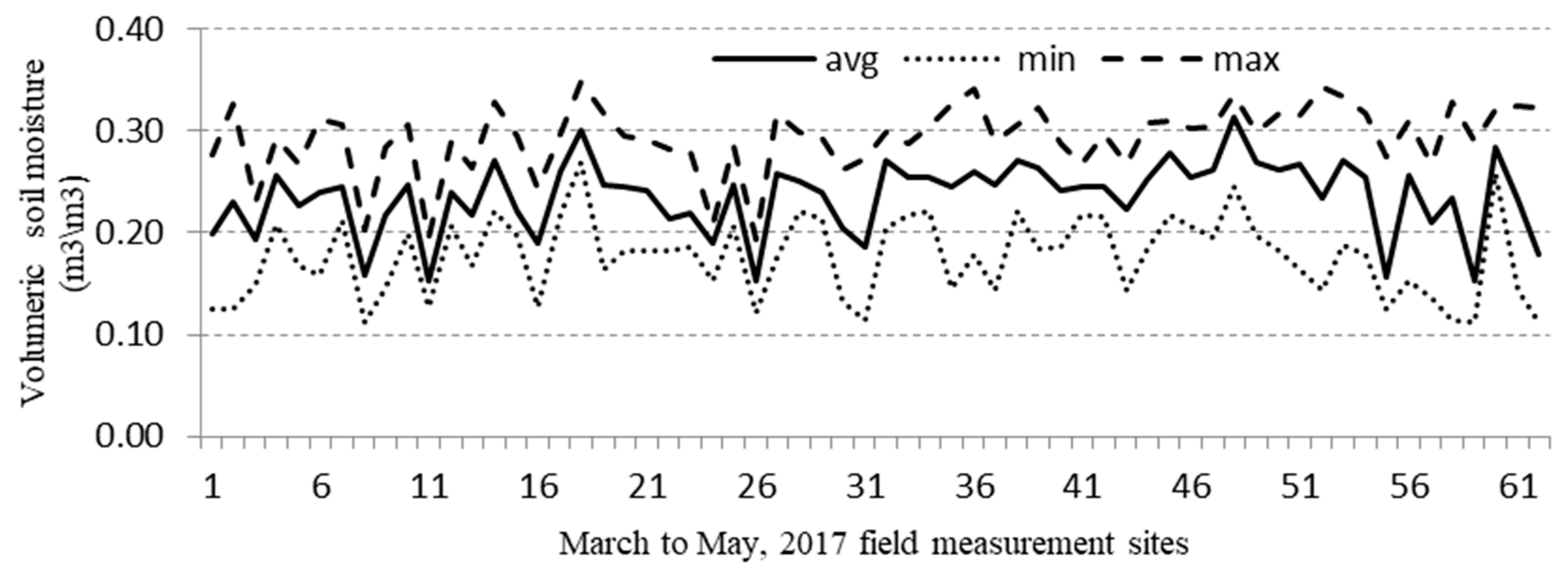
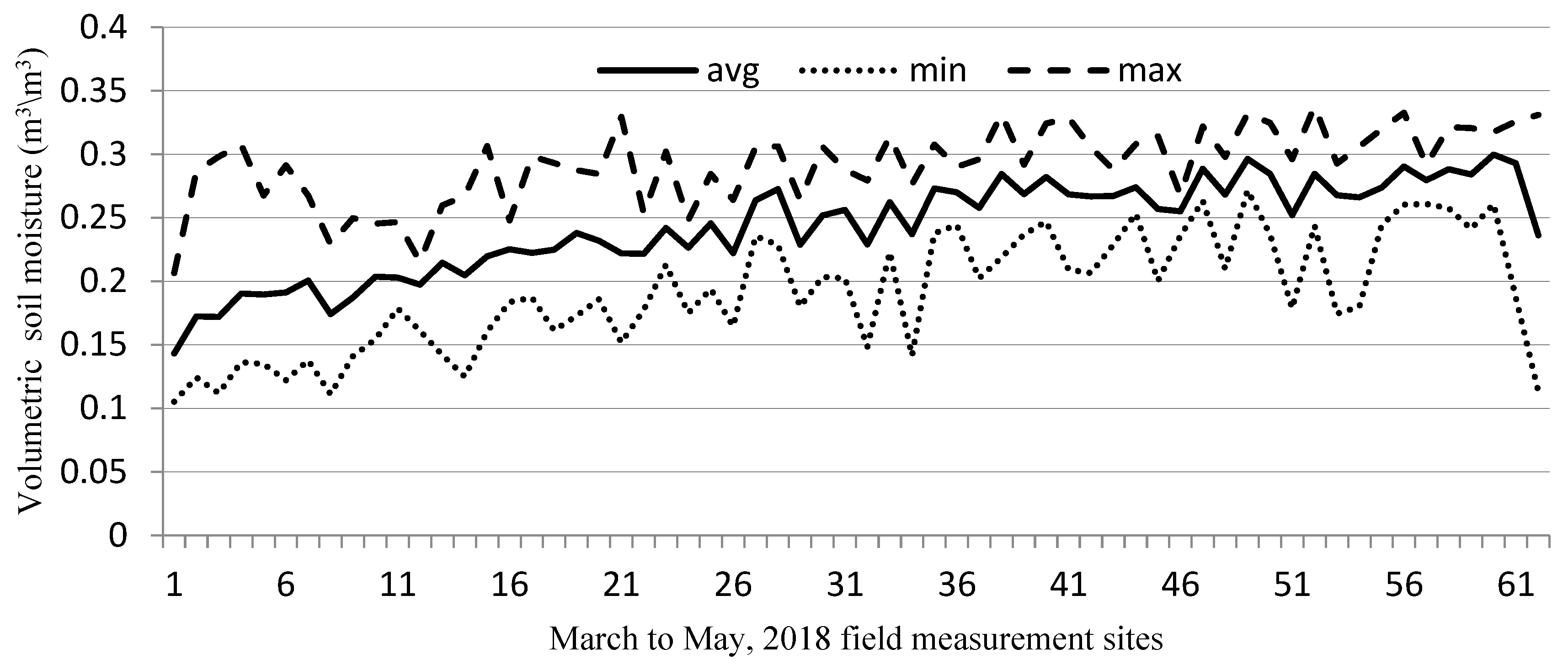
Soil moisture was estimated using the gravimetric method for all 62 samples spread over Siruguppa taluk (Figure 1) for each date of satellite pass. Mean volumetric soil moisture (${\vartheta }_v$) in the samples ranged from 0.22 m³/m³ to 0.28 m³/m³ from 4 March 2017 to 27 May 2017. Minimum ${\vartheta }_v$ varied from 0.12 m³/m³ to 0.17 m³/m³ from March 2017 to May 2017 and the maximum ${\vartheta }_v$ varied from 0.30 m³/m³ to 0.34 m³/m³, respectively (Table 2). Figure 3 illustrates the range of values that each point in the population takes above and below the mean for six dates of satellite passes during 2017. It is worth noting that Figure 3 displays the soil moisture values measured the day of the satellite passes and for this reason, the ranges of the variation of soil moisture appeared as different from those reported in Table 2. Similarly, measurements were made during 2018 at the same locations. The minimum ${\vartheta }_v$ varied from 0.11 m³/m³ to 0.15 m³/m³ and the maximum varied from 0.32 to 0.34 m³/m³ from March 2018 to May 2018, respectively. The mean ${\vartheta }_v$ was measured between 0.23 m³/m³ and 0.26 m³/m³ (Table 2). Figure 4 shows the range of values during 2018 for the seven dates of satellite passes during 2018.

3.2. Localized and Generalized Relationships

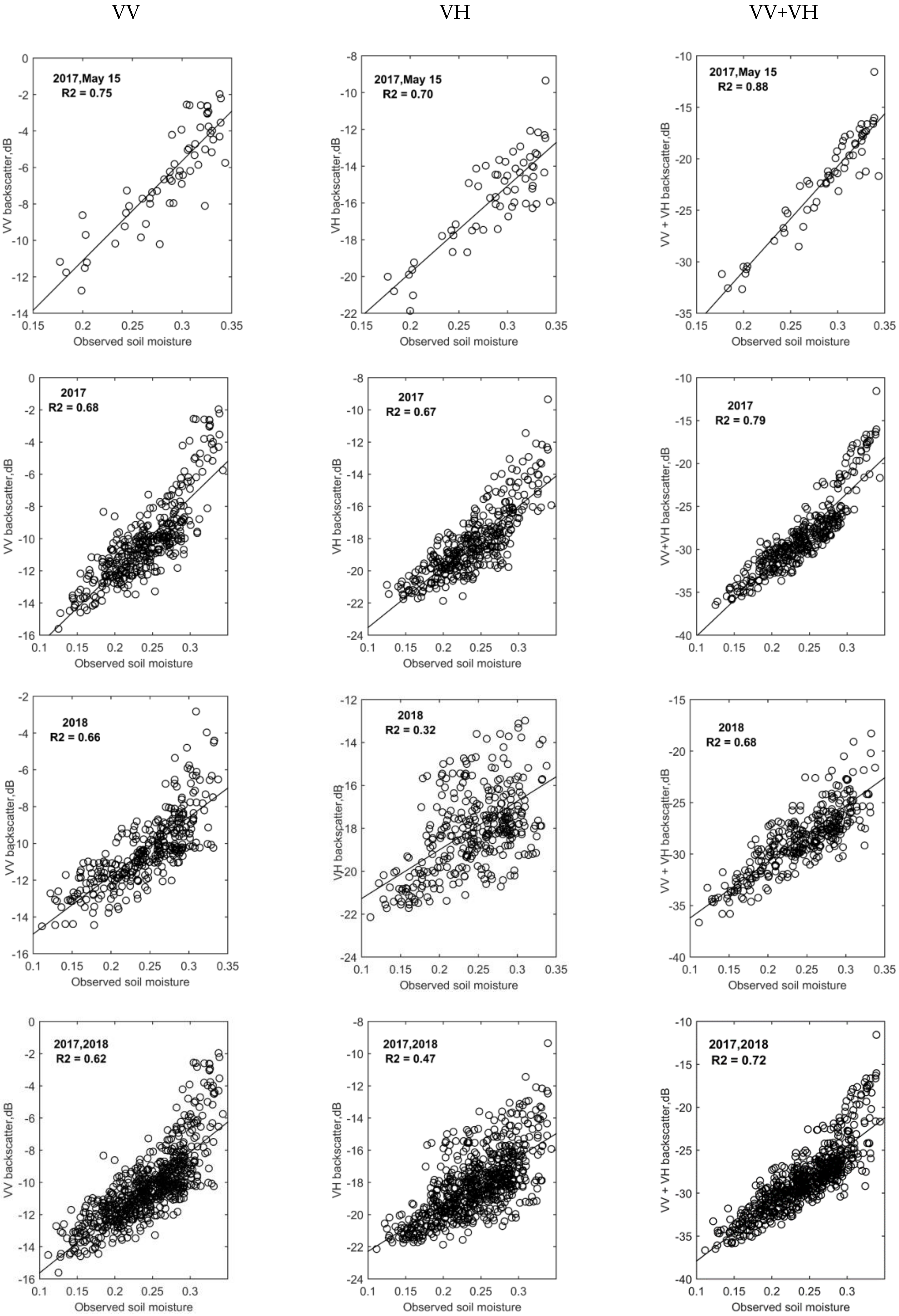
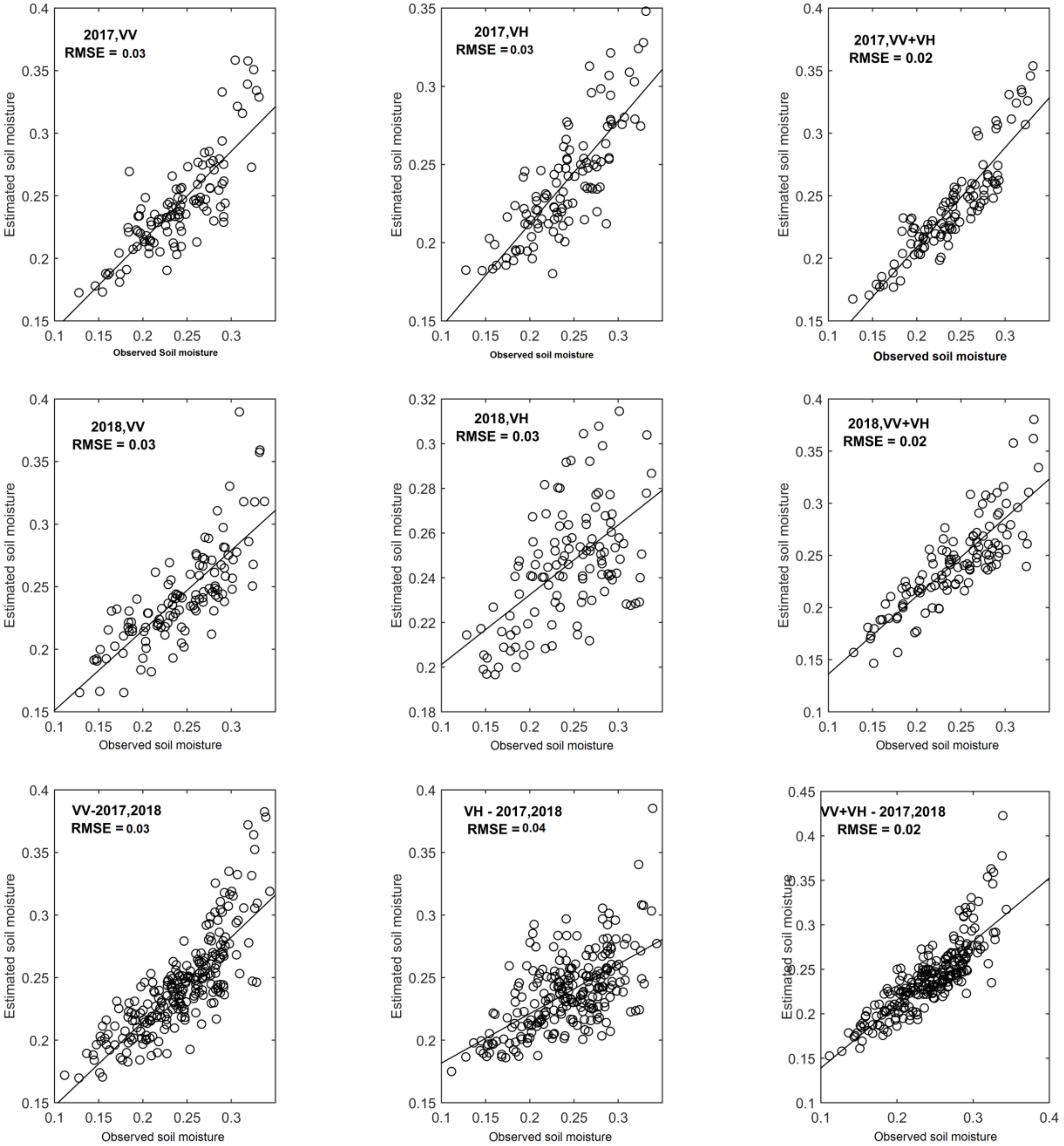
The concepts of localized and generalized relationships were used in the in situ measurements of soil moisture and SAR estimates. A relationship was localized if it was obtained using single date data points in the study area, collected both in 2017 and 2018. A generalized relationship was obtained when all the dates data points were considered in the study area (Figure 5).

The relationship for localized models showed R² ranging from 0.62 to 0.75 between ${\sigma }_{VV}^0$ and ${\vartheta }_v$, revealing a significantly strong relationship in 2017 (

Table 3. Localized relationship between soil moisture and backscatter.

Sentinel-1 Acquisition Date	${\mathbf{R}}^2\left({\mathit{\sigma }}_{\mathit{V}\mathit{V}}^0\right)$	${\mathbf{R}}^2\left({\mathit{\sigma }}_{\mathit{V}\mathit{H}}^0\right)$	${\mathbf{R}}^2({\mathit{\sigma }}_{\mathit{V}\mathit{V}}^0$$+{\mathit{\sigma }}_{\mathit{V}\mathit{H}}^0)$
4 March 2017	0.63	0.66	0.83
28 March 2017	0.65	0.65	0.87
21 April 2017	0.68	0.67	0.84
3 May 2017	0.69	0.56	0.80
15 May 2017	0.75	0.70	0.88
27 May 2017	0.62	0.43	0.71
11 March 2018	0.69	0.32	0.75
23 March 2018	0.63	0.34	0.78
4 April 2018	0.56	0.47	0.60
16 April 2018	0.64	0.33	0.72
28 April 2018	0.63	0.31	0.66
10 May 2018	0.65	0.62	0.86
22 May 2018	0.57	0.54	0.78

). As far as ${\sigma }_{VH}^0$ is concerned, it was found to have a lower R², ranging from 0.43 to 0.70. During 2018, R² values ranged from 0.56 to 0.69 for ${\sigma }_{VV}^0$ and from 0.31 to 0.62 for ${\sigma }_{VH}^0$. The linear combination of ${\sigma }_{VV}^0$ and ${\sigma }_{VH}^0$ showed higher R² values, ranging from 0.71 to 0.88 during 2017, and from 0.60 to 0.86 during 2018 (see Table 3).

Generalized relationships attempted to study the impact of seasonal effects observed in the study area due to different agroecologies (i.e., the different management and practices in a homogenous landscape).

Table 4. Generalized relationship between soil moisture and backscatter.

Year	$\mathsf{\sigma }°$	R2
2017	VV	0.68
2017	VH	0.67
2017	VV + VH	0.79
2018	VV	0.66
2018	VH	0.32
2018	VV + VH	0.62
2017, 2018	VV	0.62
2017, 2018	VH	0.47
2017, 2018	VV + VH	0.72

summarizes the R² values obtained in the individual years 2017 and 2018 along with a combination of two years for ${\sigma }_{VV}^0$, ${\sigma }_{VH}^0$ and their linear combination (${\sigma }_{VV}^0$ + ${\sigma }_{VH}^0$). The individual and combined backscatter coefficients in the two VV and VH polarizations over 2017 and 2018 pointed out a clear relationship with the in situ measurements of soil moisture.

3.3. Soil Moisture Evaluation

Multi-linear regression and linear regression were applied to determine the value of empirical constants (A, B, and T) in both the localized and generalized models.

Table 5. Empirical constants (A, B, and T) of the localized model. The total number of samples for each date was 62. The linear equation was derived using 70% of the total population.

							Validation
Sentinel-1 Image	Acquisition Date	Model	A	B	T	R2	RMSE
1	4 March 2017	$\left({\vartheta }_v\right)$$=\mathrm{A}\times {\sigma }_{\mathrm{VV}}^0$$+\mathrm{B}\times {\sigma }_{\mathrm{VH}}^0+\mathrm{T}$	0.014	0.011	0.60	0.82	0.01
2	28 March 2017	$({\vartheta }_v$$)=\mathrm{A}\times {\sigma }_{\mathrm{VV}}^0$$+\mathrm{B}\times {\sigma }_{\mathrm{VH}}^0+\mathrm{T}$	0.013	0.014	0.65	0.88	0.02
3	21 April 2017	$({\vartheta }_v$$)=\mathrm{A}\times {\sigma }_{\mathrm{VV}}^0$$+\mathrm{B}\times {\sigma }_{\mathrm{VH}}^0+\mathrm{T}$	0.011	0.015	0.65	0.84	0.01
4	3 May 2017	$({\vartheta }_v$$)=\mathrm{A}\times {\sigma }_{\mathrm{VV}}^0$$+\mathrm{B}\times {\sigma }_{\mathrm{VH}}^0+\mathrm{T}$	0.014	0.012	0.62	0.76	0.01
5	15 May 2017	$({\vartheta }_v$$)=\mathrm{A}\times {\sigma }_{\mathrm{VV}}^0$$+\mathrm{B}\times {\sigma }_{\mathrm{VH}}^0+\mathrm{T}$	0.008	0.008	0.47	0.90	0.02
6	27 May 2017	$({\vartheta }_v$$)=\mathrm{A}\times {\sigma }_{\mathrm{VV}}^0$$+\mathrm{B}\times {\sigma }_{\mathrm{VH}}^0+\mathrm{T}$	0.017	0.012	0.63	0.75	0.03
7	11 March 2018	$({\vartheta }_v$$)=\mathrm{A}\times {\sigma }_{\mathrm{VV}}^0$$+\mathrm{B}\times {\sigma }_{\mathrm{VH}}^0+\mathrm{T}$	0.016	0.008	0.57	0.82	0.02
8	23 March 2018	$({\vartheta }_v$$)=\mathrm{A}\times {\sigma }_{\mathrm{VV}}^0$$+\mathrm{B}\times {\sigma }_{\mathrm{VH}}^0+\mathrm{T}$	0.013	0.008	0.52	0.84	0.02
9	4 April 2018	$({\vartheta }_v$$)=\mathrm{A}\times {\sigma }_{\mathrm{VV}}^0$$+\mathrm{B}\times {\sigma }_{\mathrm{VH}}^0+\mathrm{T}$	0.022	0.004	0.55	0.76	0.02
10	16 April 2018	$({\vartheta }_v$$)=\mathrm{A}\times {\sigma }_{\mathrm{VV}}^0$$+\mathrm{B}\times {\sigma }_{\mathrm{VH}}^0+\mathrm{T}$	0.015	0.008	0.53	0.77	0.03
11	28 April 2018	$({\vartheta }_v$$)=\mathrm{A}\times {\sigma }_{\mathrm{VV}}^0$$+\mathrm{B}\times {\sigma }_{\mathrm{VH}}^0+\mathrm{T}$	0.022	0.010	0.67	0.70	0.02
12	10 May 2018	$({\vartheta }_v$$)=\mathrm{A}\times {\sigma }_{\mathrm{VV}}^0$$+\mathrm{B}\times {\sigma }_{\mathrm{VH}}^0+\mathrm{T}$	0.016	0.017	0.74	0.90	0.02
13	22 May 2018	$({\vartheta }_v$$)=\mathrm{A}\times {\sigma }_{\mathrm{VV}}^0$$+\mathrm{B}\times {\sigma }_{\mathrm{VH}}^0+\mathrm{T}$	0.014	0.019	0.76	0.78	0.02

and

Table 6. Empirical constants (A, B, and T) of the generalized model. The total number of samples for 2017 was 368, for 2018 it was 427, and for a combination of 2017 and 2018, it was 795. The linear equations were derived using 70% of the total sample of each year and combined year.

							Validation
Year	$\mathsf{\sigma }°$	Model	$A$	B	T	R2	RMSE
2017	VV	$({\vartheta }_v$$)=\mathrm{A}·{\sigma }_{\mathrm{VV}}^0$ + T	0.015	-	0.39	0.70	0.03
2017	VH	$({\vartheta }_v$$)=\mathrm{B}·{\sigma }_{\mathrm{VH}}^0$ + T	-	0.017	0.56	0.67	0.03
2017	VV + VH	$({\vartheta }_v$$)=\mathrm{A}·{\sigma }_{\mathrm{VV}}^0$$+\mathrm{B}·{\sigma }_{\mathrm{VH}}^0$ + T	0.009	0.009	0.51	0.80	0.02
2018	VV	$({\vartheta }_v)=\mathrm{A}·{\sigma }_{\mathrm{VV}}^0$ + T	0.019	-	0.44	0.60	0.03
2018	VH	$({\vartheta }_v$$)=\mathrm{B}·{\sigma }_{\mathrm{VH}}^0$ + T	-	0.014	0.50	0.32	0.03
2018	VV + VH	$({\vartheta }_v$$)=\mathrm{A}·{\sigma }_{\mathrm{VV}}^0$$+\mathrm{B}·{\sigma }_{\mathrm{VH}}^0$ + T	0.016	0.009	0.58	0.70	0.02
2017, 2018	VV	$({\vartheta }_v)=\mathrm{A}·{\sigma }_{\mathrm{VV}}^0$ + T	0.016	-	0.41	0.60	0.03
2017, 2018	VH	$({\vartheta }_v$$)=\mathrm{B}·{\sigma }_{\mathrm{VH}}^0$ + T		0.016	0.59	0.50	0.04
2017, 2018	VV + VH	$({\vartheta }_v$$)=\mathrm{A}·{\sigma }_{\mathrm{VV}}^0$$+\mathrm{B}·{\sigma }_{\mathrm{VH}}^0$ + T	0.011	0.009	0.59	0.70	0.02

summarize the results. Each localized model comprises images from one date of pass over of the study area, totaling 39 equations from March 2017 to May 2018, and considering individual ${\sigma }_{VV}^0$, ${\sigma }_{VH}^0$, and their linear combination ${\sigma }_{VV}^0$ + ${\sigma }_{VH}^0$. Each generalized model combines all images acquired during a year for individual ${\sigma }_{VV}^0$, ${\sigma }_{VH}^0$ and linear combination ${\sigma }_{VV}^0$ + ${\sigma }_{VH}^0$. Three models were obtained for each year 2017 and 2018 and three additional models using all the images used in the study, making it a total of nine generalized models. For the localized model, 40 samples for calibration and 22 samples for validation were used during 2017 and 2018 (N = 62). The model calibration for individual dates (localized models) with combined backscatter coefficient (${\sigma }_{VV}^0$ + ${\sigma }_{VH}^0$) during the study years of 2017 and 2018 estimated an R² ranging from 0.91 to 0.70 and RSE ranging from 0.03 to 0.01.

As far as generalized models are concerned, N = 368 points were used in 2017, 258 for calibration, and 110 for validation, and N = 427 in 2018, with 299 for calibration and 128 for validation. The total number of points for both years was N = 795, with 557 used for calibration and 238 for validation. The nine linear equations modeled each backscatter coefficient ${\sigma }_{VV}^0$, ${\sigma }_{VH}^0$ and a linear combination of both (${\sigma }_{VV}^0$ + ${\sigma }_{VH}^0$) for each year (2017, 2018) and 2017 and 2018 put together. Table 6 summarizes the R² values modeled from ${\sigma }_{VV}^0$ and ${\sigma }_{VH}^0$ as a function of (${\vartheta }_v$) during 2017 and 2018. RSE was 0.03 for 2017, 2018 from ${\sigma }_{VV}^0$, and 0.03 and 0.04 from ${\sigma }_{VH}^0$ for 2017 and 2018, respectively. A linear combination of both backscatter coefficients during 2017 and 2018 showed an R² of 0.80 and 0.70, respectively. The RSE values were 0.02. The backscatter coefficient from each polarization and a linear combination of both polarizations put together for two years were also attempted. The R² from ${\sigma }_{VV}^0$ was 0.60 with a RSE of 0.03 and from ${\sigma }_{VH}^0$ it was 0.50 with a RSE 0.03. The R² from a linear combination of both polarizations (${\sigma }_{VV}^0$ + ${\sigma }_{VH}^0$) was 0.70 with a RSE of 0.02.

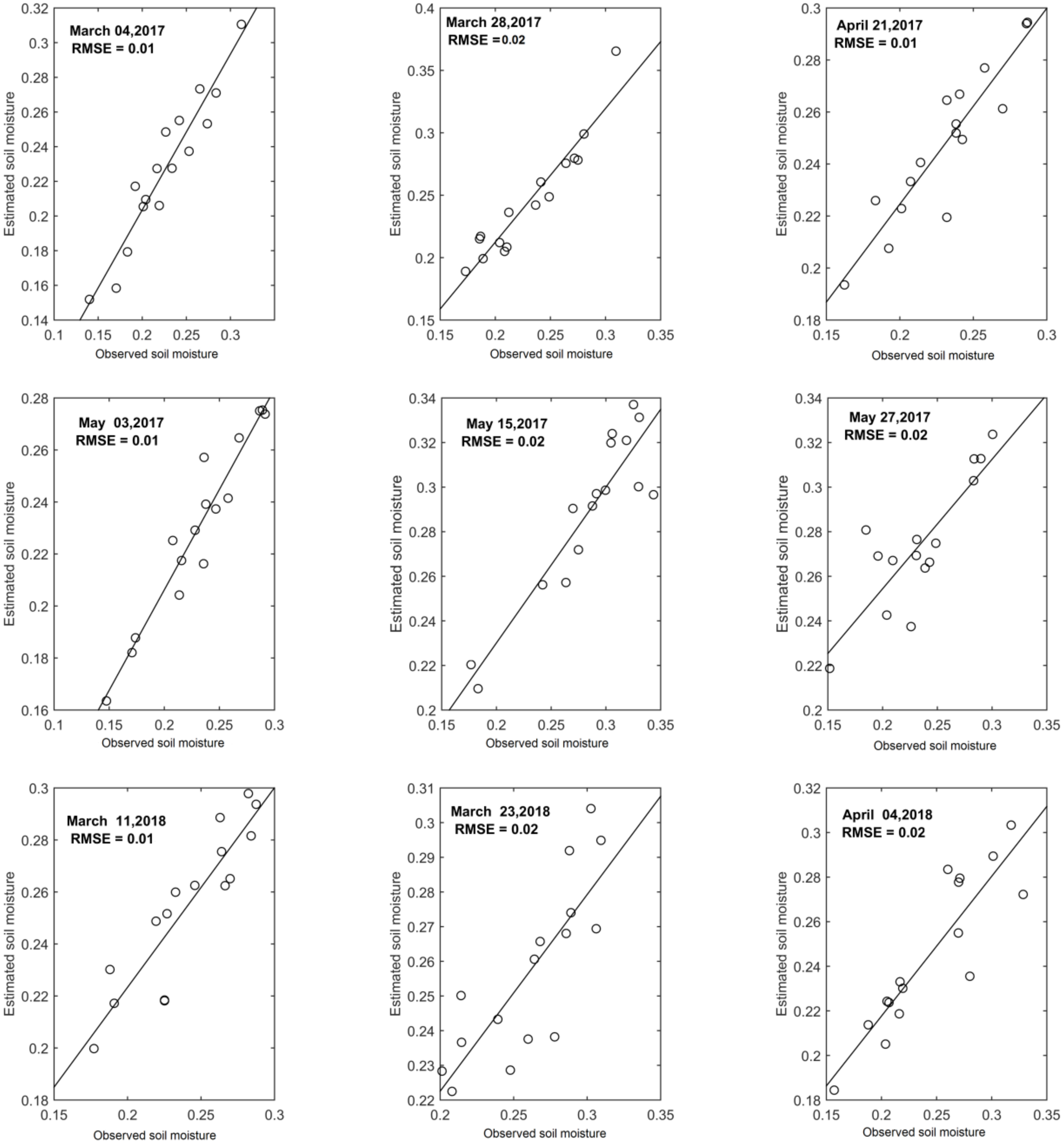
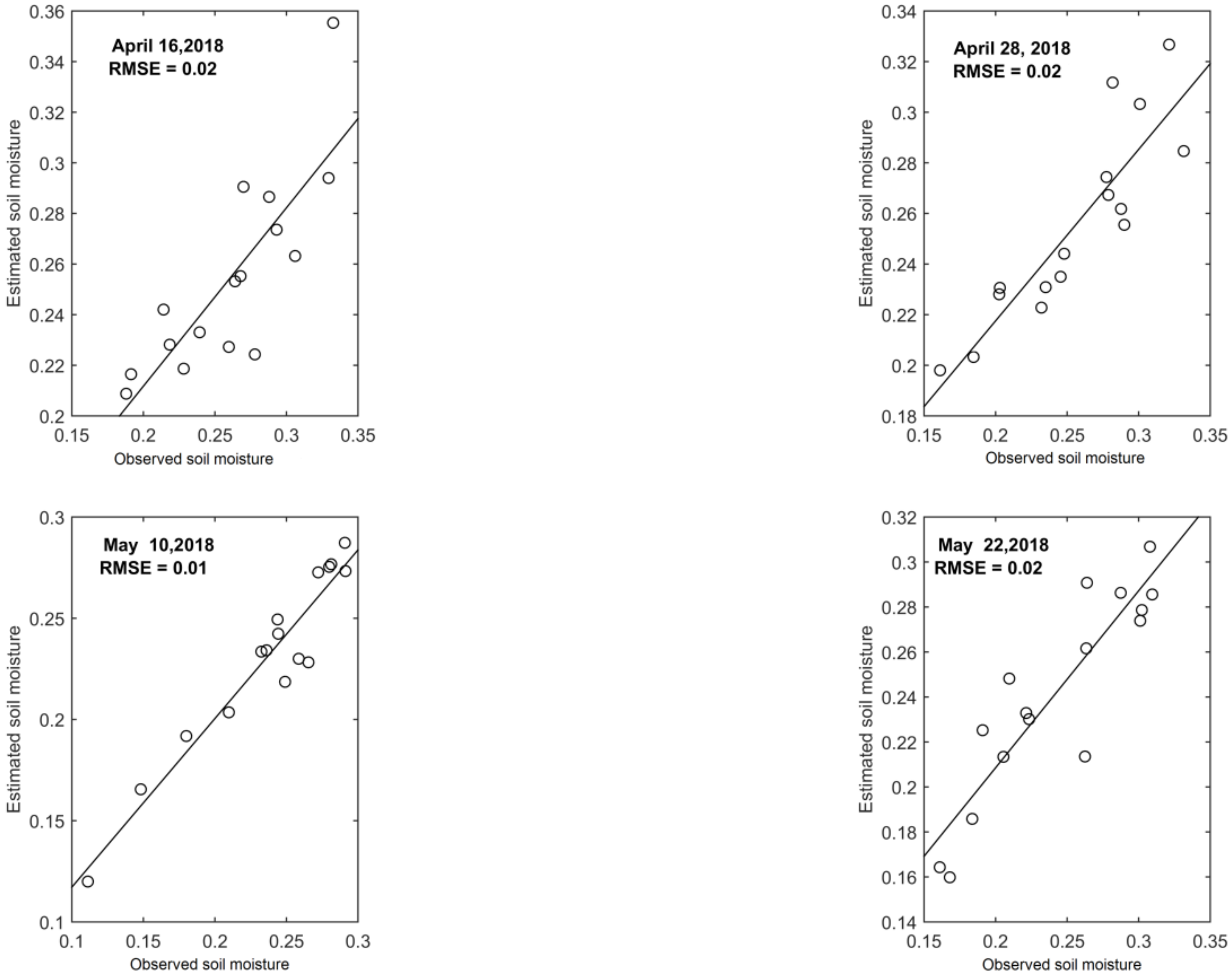
Model validation was done for individual dates from a linear combination of the two polarizations. Table 5 and Figure 6 summarize the RMSE values for 2017 and 2018. The nine generalized models were also validated and the RMSE values are reported in Table 6 and Figure 7.

4. Discussion

Accurate estimation of ${\vartheta }_v$ was envisaged using a linear equation of ${\sigma }_{VV}^0$ and ${\sigma }_{VH}^0$ radar cross section from bare agricultural soils. A thorough data collection campaign was undertaken during 2017 and 2018, synchronizing with the pass of the satellite. Bare soil areas were mostly post-harvest cropped areas with little or no crop residue, depending on the crop sown. In the study area, 50% of the agricultural land comprises rice cropped and irrigated from a seasonal stream. Sentinel-1 SAR, dual polarized imagery was used to estimate soil moisture over bare soils using a semi-empirical model. Model parameters were estimated using linear and multi-linear regression. Performance evaluation was conducted based on a 70:30 ratio of sampled points and low RMSE was found between the observed and estimated soil moisture, when a linear relationship between ${\sigma }_{VV}^0$ and ${\sigma }_{VH}^0$ was combined for 2017 and 2018.

4.1. Relationship between ${\sigma }_{VV}^0$ and ${\sigma }_{VH}^0$ with Observed Data

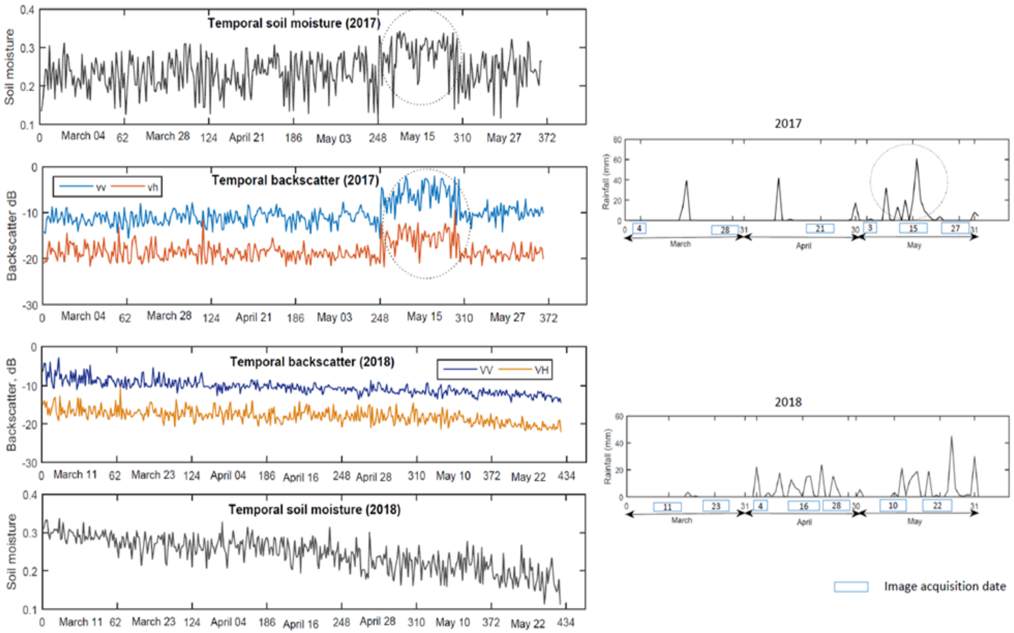
Soil moisture data were collected over two years (2017 to 2018) during the dry summer season from March to May from the 62 plots on the dates of the satellite passes. The relationship between ${\sigma }_{VV}^0$, ${\sigma }_{VH}^0$, and observed soil moisture by individual dates of the satellite pass (13 images) showed that in both years, the backscatter and observed soil moisture had a significant positive correlation [2,10,27,28]. In both years, VV polarization had a higher backscatter dB value than VH polarization. In cross-polarization (VH), signal attenuation occurs due to volumetric scattering [29]. In 2017, soil moisture constantly increased from 4 March to 27 April. The R² between radar backscattering coefficient and in situ measurements of soil moisture is reported in Table 3. A sudden increase in R² (VV) can be observed on 15 May, corresponding to the consecutive rainfall events that occurred during the three days before the date of the satellite pass (Figure 8). This means that there is a better correlation for high values of soil moisture, probably because under this condition, the radar backscattering coefficient’s dependence on soil moisture is more important than it is on surface roughness.

Similarly, an unexpected increase in ${\sigma }_{VH}^0$ was observed (Figure 5). 27 May 2017 (Table 3) had a low R² value from ${\sigma }_{VH}^0$ compared to the rest of the dates due to the rainfall event (Figure 8), weeds or crop residue moisture [24]. In 2018, R² for the relationship between ${\sigma }_{VV}^0$ and observed soil moisture was significant during March because of residual soil moisture (i.e., the crop residual moisture influenced the radar backscattering coefficient, Table 3). Residual soil moisture was low on 4 April and 22 May due to evaporative demand and higher between 16 April and 10 May due to consecutive rainfall events (Figure 8). R² did not decrease from March to May, probably due to irregular changes in crop residue moisture, since ${\sigma }_{VH}^0$ is sensitive to it [24]. The R² values from ${\sigma }_{VH}^0$ during March were relatively low despite no rainfall in the month because of residual soil moisture from the previous crop. The cumulative moisture due to rainfall during April is reflected in the low R² of 16 April and 28 April (Figure 8). During May, high R² values were due to bare soils. A linear combination of ${\sigma }_{VV}^0$ and ${\sigma }_{VH}^0$ during each date in 2017 produced higher R² compared to R² from individual polarization. This shows that the addition of ${\sigma }_{VV}^0$ and ${\sigma }_{VH}^0$ or vice versa improves the backscatter and soil moisture relationship rather than a single relationship with different polarization (Table 3). A similar relationship existed during 2018 from a linear combination of ${\sigma }_{VV}^0$ and, which improved R² significantly (Table 3).

4.2. Localized and Generalized Relationships

To operationalize the accurate estimation of soil moisture for decision making, a global relationship was envisaged considering all dates during the dry season. The R² value of global relationship from VV polarization during 2017 was 0.68, which was higher than the mean of the local relationships. The generalized relationship was found to be more useful for an accurate soil moisture estimate. In addition, R² for the generalized relationship performed better than the mean of the localized relationship (0.67) with VH polarization. The scenario during 2018 from VV polarization was more influenced by rainfall events in the dry season. The R² values ranged from 0.56 to 0.69 with a mean of 0.62 from localized relationships and 0.66 from the generalized relationship, which was more than the local mean. R² was very low from VH polarization due to cumulative moisture from rainfall events. However, the generalized relationship produced a lower R² than the mean localized relationship for VH in 2018 (see Table 3 and Table 4). The usefulness of a generalized relationship was exhibited with a consistent increase in the accuracy of the soil moisture estimates over two years. The relationship from VV and VH polarization during 2017 showed significantly lower R² than the linear combination of VV and VH during the same year. Similarly, also during 2018, R² was significantly higher than the individual polarization. Finally, the best relationship was obtained when the linear combination of two polarizations was combined (appended) for the two years 2017 and 2018, than from single polarizations combined for the two years. It was inferred that generalized relationships are more promising in terms of building a model compared to localized relationships, which may not relate to the entire population.

4.3. Modeling the Relationships

The relationships of localized and generalized modeling were explored and tested for multicollinearity, especially linear combination models ${\sigma }_{VV}^0$ + ${\sigma }_{VH}^0$. Multicollinearity is a statistical phenomenon in which two or more predictor variables in a multiple regression model are highly correlated [30]. To detect multicollinearity, we used an indicator called variance inflation factor (VIF), which is a tool to measure and quantify how much the variance is inflated [30]. If any of the model’s VIF values exceed 5 or 10, it is an indication that the associated regression coefficient is poorly estimated because of multicollinearity [31]. The P value indicates statistical significance for independent variable contribution in the model, which is explained in Section 2.4.3.

For generalized models, nine different types of linear relationships were explored with ${\sigma }_{VV}^0$ and ${\sigma }_{VH}^0$ data (Table 6) during 2017 and 2018. In 2017, among the three possible models ${\sigma }_{VV}^0$, ${\sigma }_{VH}^0$ and, ${\sigma }_{VV}^0$ + ${\sigma }_{VH}^0$, individual models ${\sigma }_{VV}^0$ and ${\sigma }_{VH}^0$ showed a low RSE and the p value was statistically significant. When ${\sigma }_{VH}^0$ was added to ${\sigma }_{VV}^0$, the RSE was lower than in the individual models. This indicates a very good relationship with a low VIF as well as p value for both backscatter coefficients. Similar results were observed in 2018. Generalized models derived by combining two years (2017 and 2018) of data showed similar results as individual year models. This study also showed that the linear combination equations from the localized models also performed well with low VIF (<2) and a p value statistically significant for both backscatter coefficients (

Table 7. Analysis of variance in the generalized model.

Year	$(\mathsf{\sigma }°)\mathbf{Variable}$	t Value	$\mathit{P}\mathit{r}(>\left|\mathit{t}\right| )$	$\mathit{V}\mathit{I}\mathit{F}$
2017	VV	24.24	<2 × 10−16 ***	-
2017	VH	23.24	<2 × 10−16 ***	-
2017	VV, VH	12.17, 11.20	<2 × 10−16 ***	2.11
2018	VV	21.23	<2 × 10−16 ***	-
2018	VH	11.98	<2 × 10−16 ***	-
2018	VV, VH	20.76, 11.50	<2 × 10−16 ***	1.10
2017, 2018	VV	29.49	<2 × 10−16 ***	-
2017, 2018	VH	24.31	<2 × 10−16 ***	-
2017, 2018	VV, VH	21.57, 16.32	<2 × 10−16 ***	1.40

*** p value < 0.001.

and

Table 8. Analysis of variance in the localized model.

Date	$(\mathsf{\sigma }°)\mathbf{Variable}$	t Value	$\mathit{P}\mathit{r}(>\left|\mathit{t}\right| )$	$\mathit{V}\mathit{I}\mathit{F}$
4 March 2017	VV, VH	4.63, 7.54	<2 × 10−16 ***	1.36
28 March 2017	VV, VH	8.24, 8.04	<2 × 10−16 ***	1.30
21 April 2017	VV, VH	6.93,9.02	<2 × 10−16 ***	1.54
3 May 2017	VV, VH	7.39, 4.34	<2 × 10−16 ***	1.63
15 May 2017	VV, VH	6.93, 5.02	<2 × 10−16 ***	1.71
27 May 2017	VV, VH	5.03, 5.17	<2 × 10−16 ***	1.12
11 March 2018	VV, VH	10.45, 6.07	<2 × 10−16 ***	1.09
23 March 2018	VV, VH	11.25, 6.00	<2 × 10−16 ***	1.10
4 April 2018	VV, VH	10.19, 1.94	<2 × 10−16 ***	1.14
16 April 2018	VV, VH	9.17, 4.47	<2 × 10−16 ***	1.11
28 April 2018	VV, VH	9.10, 4.12	<2 × 10−16 ***	1.0
10 May 2018	VV, VH	10.69, 11.09	<2 × 10−16 ***	1.27
22 May 2018	VV, VH	6.66, 6024	<2 × 10−16 ***	1.26

*** p value < 0.001.

).

A collinearity test on the generalized and localized models showed that the VIF for a linear combination of both backscatter coefficients (VV + VH) was <3. Hence, these models are non-collinear. All models showed low p value, indicating that both backscatter coefficients made meaningful addition to the models. During modeling relationships with a linear combination of individual backscatter coefficient, it was inferred that the individual backscatter coefficients were non-collinear, contributing to R² independently. It was found that the localized models from individual dates varied over time, and any one equation with a low RSE and VIF may not represent the whole season. In addition, the generalized models produced lower RSE representing the whole season, and were hence better than each localized model.

4.4. Validation of Models

Models were validated using 30% of the sampled points. Results for the localized models are summarized in Table 5. In 2017, the lowest RMSE (0.01) was found on 21 April. Figure 8 shows that no rainfall or very weak rainfall was observed on this day. An increase in RMSE was observed on 15 May. Similarly, in 2018, the lowest RMSE was observed on 23 March and the highest (0.03) on 16 April 2018, probably due to the increase in rainfall. The results seem to show that the RMSE of the models is related to the amount of rainfall. Localized models performed better in drier soils.

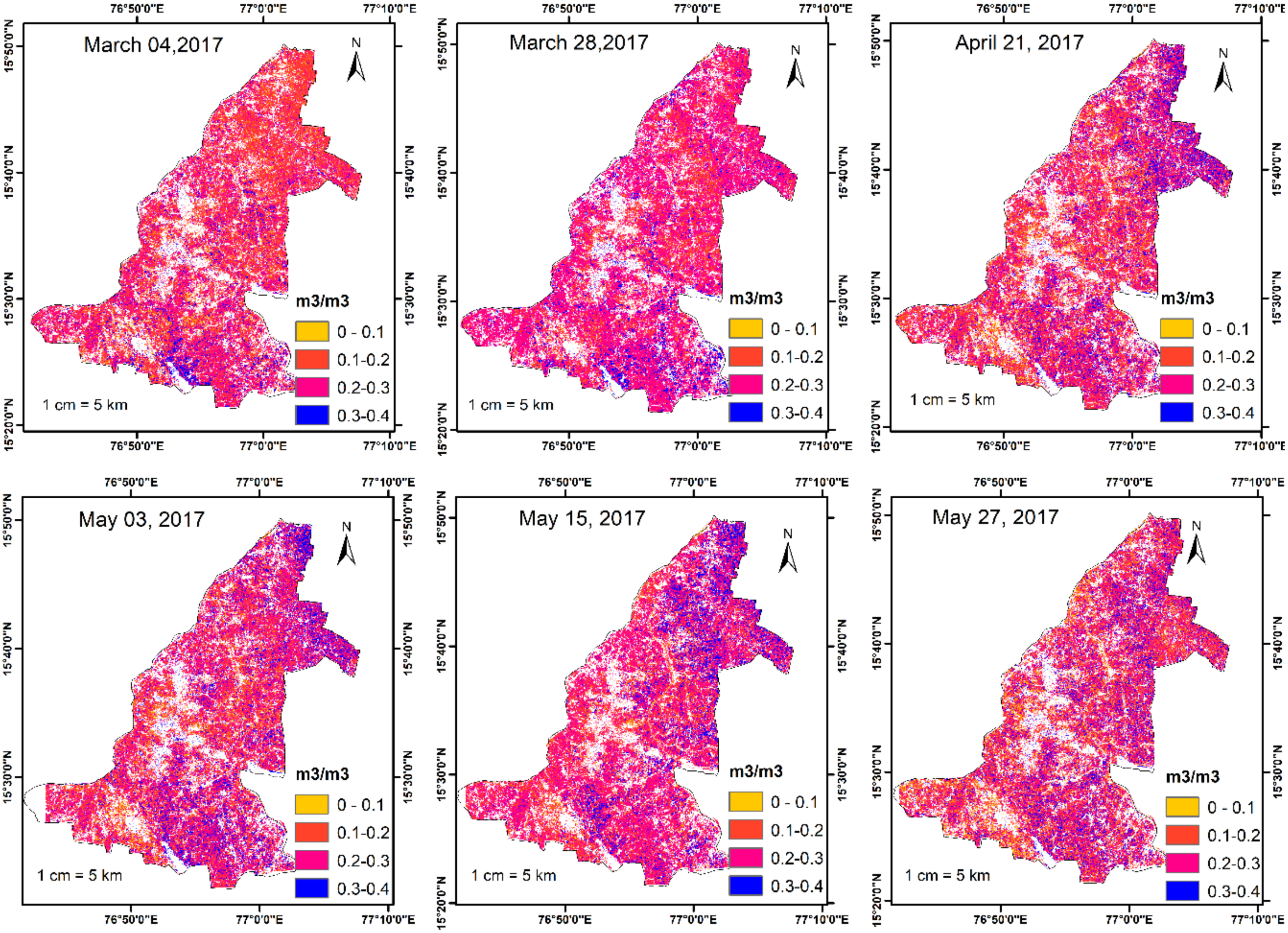
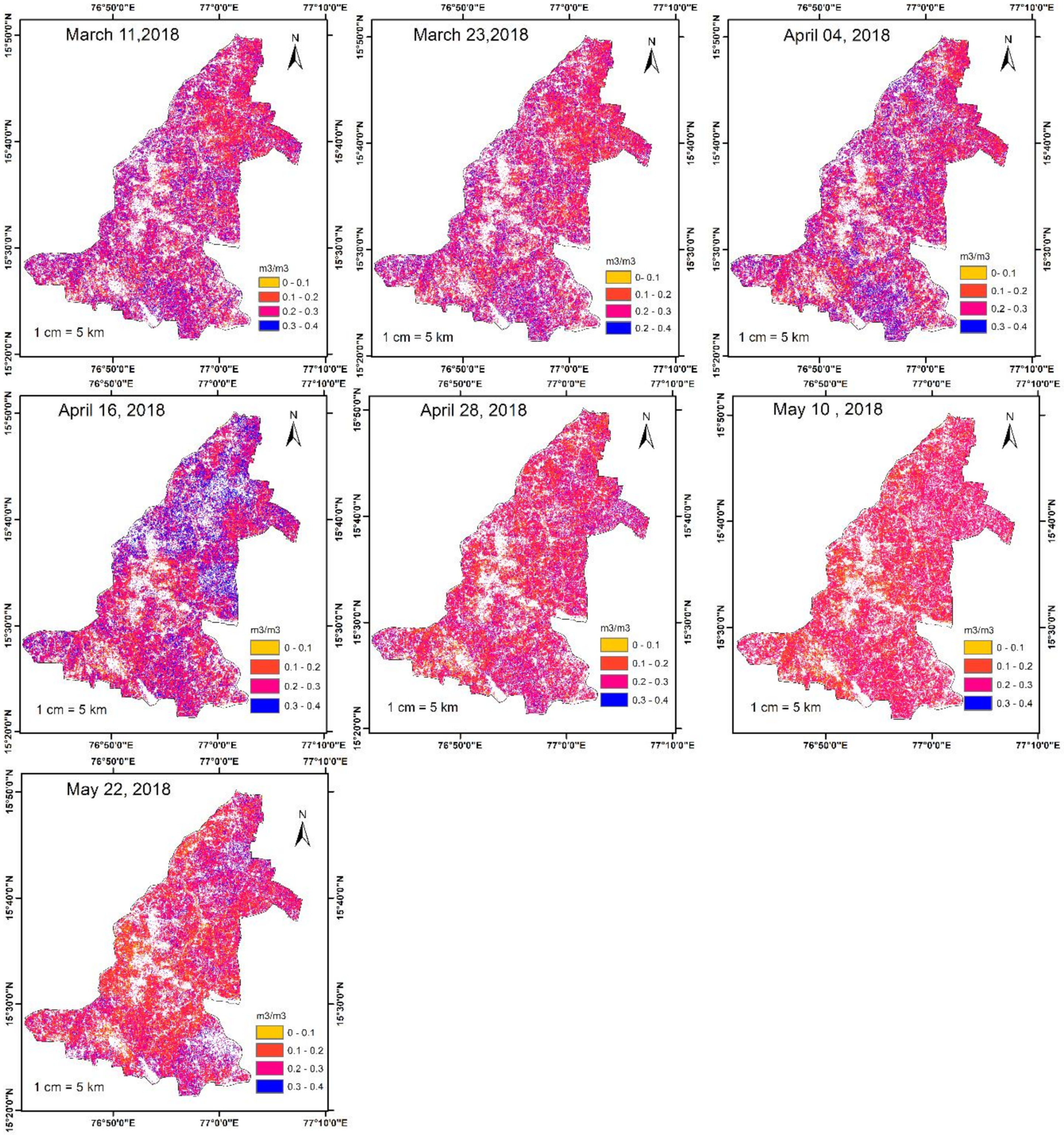
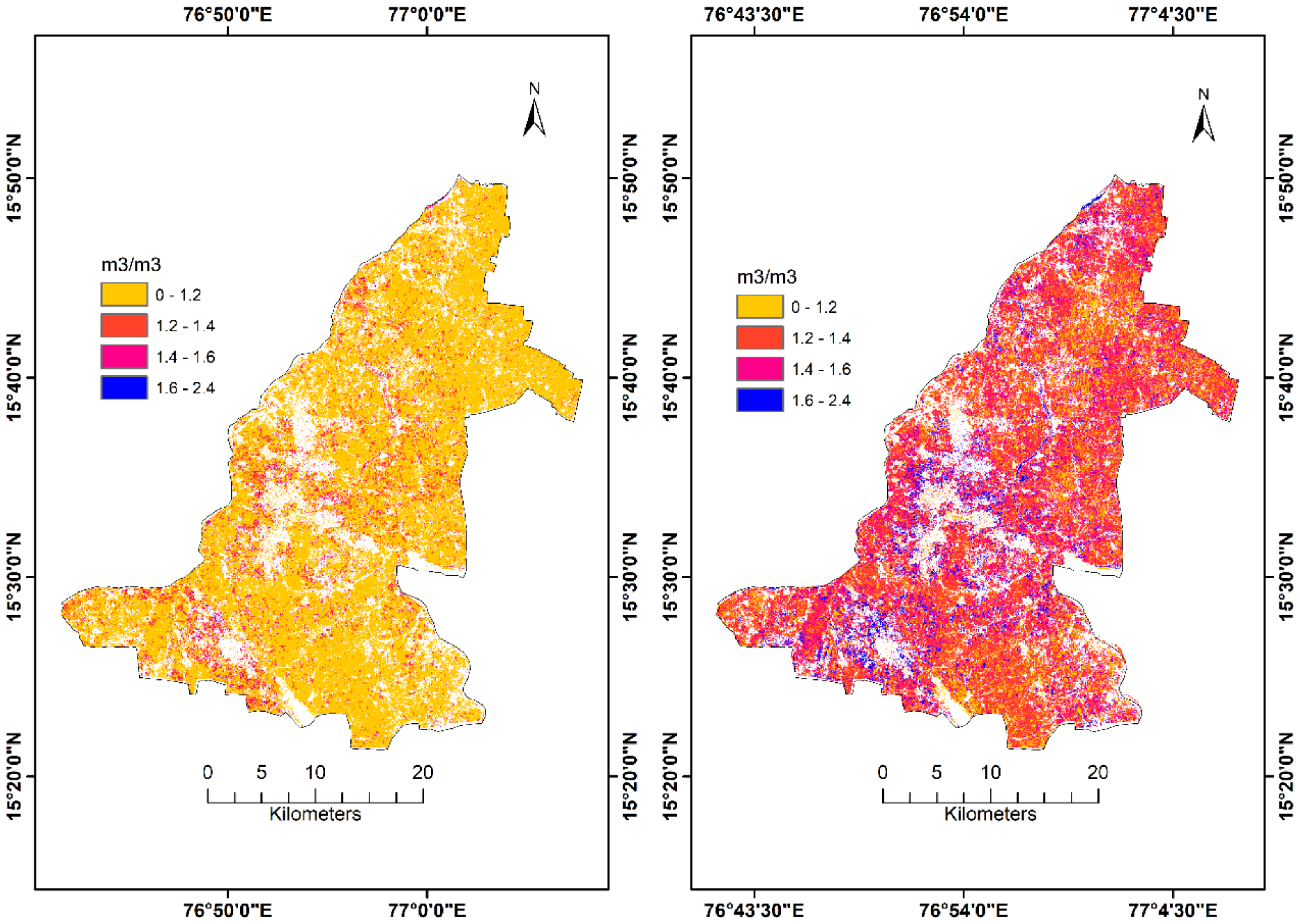
As far as the generalized models are concerned, the validation results showed that generalized models obtained using co-polar ${\sigma }_{VV}^0$ data provided a lower RMSE than those based on cross-polar ${\sigma }_{VH}^0$ data for both 2017 and 2018 and taking all data acquired from 2017 to 2018. We also found that the linear combination of both co-polar and cross-polar backscattering coefficients always provided a lower RMSE than the models using only one polarization. The best results came when using the linear combination of polarizations and all the data acquired along the two years, resulting in an RMSE of 0.02 (Table 6). This globalized model was used to produce maps of soil moisture and its spatial variability (Figure 9, Figure 10 and Figure 11). This is probably the most important result, as a simple multi-linear model using both co-polar and cross-polar Sentinel-1 data acquired over long time periods can reproduce the spatial variability of soil moisture.

5. Conclusions

This study aimed to accurately estimate the soil moisture of bare, post-harvest agricultural areas collected from Siruguppa taluk (sub-district) in the Karnataka state of India. Fifty percent of this agricultural area is grown with rice that is irrigated by seasonal canal irrigation. An accurate estimate of volumetric soil moisture (${\vartheta }_v$) was envisaged using a semi-empirical model based on a linear equation of co-polarized and cross-polarized radar cross section obtained by Sentinel-1 images. A thorough data collection campaign was undertaken during 2017 and 2018 during the pass of the satellite.

Both localized and generalized models were developed using Sentinel-1 image independently and all images together, respectively. Results indicate that the accuracy of the soil moisture estimates increased when using both co-polar and cross-polar images instead of only ${\sigma }_{VV}^0$ or ${\sigma }_{VH}^0$, independently.

The use of localized models revealed that the RMSE of soil moisture estimates decreased corresponding to dry periods, with little or no rainfall. This indicates that better estimates of soil moisture can be obtained for drier soils. Coming to globalized models, soil moisture estimates with lower RMSE were observed when merging all data acquired in 2017 and 2018, and co-polar and cross-polar images, with a R² of 0.7 and RMSE of 0.02. The availability of a large amount of in situ data collected over a large area demonstrated that a generalized linear model based on the joint use of co-polar and cross-polar C-band SAR images acquired for a long time period, with a short revisiting time of twelve days, could capture spatial variability in soil moisture. This is an important result as the availability of Sentinel-1 data can provide farmers with timely and accurate estimates of soil moisture and enable the mapping of its spatial variability by using simple semi-empirical models. This information, when provided in the immediate weeks and months preceding the cropping season, could be very crucial in determining planting dates and assessing early season plant growth, thereby playing a key role in influencing productivity.

References

1. Barrett, B.W.; Dwyer, E.; Whelan, P. Soil Moisture Retrieval from Active Spaceborne Microwave Observations: An Evaluation of Current Techniques. Remote Sens. 2009, 1, 210–242. [Google Scholar] [CrossRef] [Green Version]
2. Huang, S.; Ding, J.; Zou, J.; Liu, B.; Zhang, J.; Chen, W. Soil Moisture Retrival Based on Sentinel-1 Imagery under Sparse Vegetation Coverage. Sensors 2019, 19, 589. [Google Scholar] [CrossRef] [PubMed] [Green Version]
3. Thoma, D.P.; Moran, M.S.; Bryant, R.; Rahman, M.; Holifield-Collins, C.D.; Skirvin, S.; Sano, E.E.; Slocum, K. Comparison of four models to determine surface soil moisture from C-band radar imagery in a sparsely vegetated semiarid landscape. Water Resour. Res. 2006, 42, W01418. [Google Scholar] [CrossRef] [Green Version]
4. Romshoo, S.; Taikan, O.; Katumi, M. C-band radar for soil moisture estimation under agricultural conditions. IEEE Int. Geosci. Remote Sens. Symp. 2002, 4, 2217–2219. [Google Scholar] [CrossRef]
5. Suni, T.; Guenther, A.; Hansson, H.; Kulmala, M.; Andreae, M.; Arneth, A.; Artaxo, P.; Blyth, E.; Brus, M.; Ganzeveld, L.; et al. The significance of land-atmosphere interactions in the Earth system—iLEAPS achievements and perspectives. Anthropocene 2015, 12, 69–84. [Google Scholar] [CrossRef] [Green Version]
6. Verhoest, N.E.C.; Lievens, H.; Wagner, W.; Álvarez-Mozos, J.; Moran, M.S.; Mattia, F. On the Soil Roughness Parameterization Problem in Soil Moisture Retrieval of Bare Surfaces from Synthetic Aperture Radar. Sensors 2008, 8, 4213–4248. [Google Scholar] [CrossRef] [Green Version]
7. Dubois, P.C.; van Zyl, J.; Engman, T. Measuring soil moisture with imaging radars. IEEE Trans. Geosci. Remote Sens. 1995, 33, 915–926. [Google Scholar] [CrossRef] [Green Version]
8. Fung, A.; Li, Z.; Chen, K. Backscattering from a randomly rough dielectric surface. IEEE Trans. Geosci. Remote Sens. 1992, 30, 356–369. [Google Scholar] [CrossRef]
9. Haider, S.S.; Said, S.; Kothyari, U.C.; Arora, M.K. Soil moisture estimation using ERS 2 SAR data: A case study in the Solani River catchment/Estimation de l’humidité du sol grâce à des données ERS-2 SAR: Étude de cas dans le bassin de la rivière Solani. Hydrol. Sci. J. 2004, 49, 334. [Google Scholar] [CrossRef] [Green Version]
10. Baghdadi, N.; Aubert, M.; Cerdan, O.; Franchisteguy, L.; Viel, C.; Martin, E.; Zribi, M.; Desprats, J.-F.; Eric, M. Operational Mapping of Soil Moisture Using Synthetic Aperture Radar Data: Application to the Touch Basin (France). Sensors 2007, 7, 2458–2483. [Google Scholar] [CrossRef]
11. Rao, S.S.; Pandey, A.K.; Das, S.N.; Nagaraju, M.S.S.; Venugopal, M.V.; Rajankar, P.; Laghate, P.; Reddy, M.S.; Joshi, A.K.; Sharma, J.R. Modified Dubois Model for Estimating Soil Moisture with Dual Polarized SAR Data. J. Indian Soc. Remote Sens. 2013, 41, 865–872. [Google Scholar] [CrossRef]
12. Alexakis, D.D.; Mexis, F.-D.K.; Vozinaki, A.-E.K.; Daliakopoulos, I.N.; Tsanis, I. Soil Moisture Content Estimation Based on Sentinel-1 and Auxiliary Earth Observation Products. A Hydrological Approach. Sensors 2017, 17, 1455. [Google Scholar] [CrossRef] [PubMed] [Green Version]
13. Conde, V.; Nico, G.; Catalao, J. Comparison of In-Field Measurements and INSAR Estimates of Soil Moisture: Inversion Strategies of Interferometric Data. In Proceedings of the IGARSS 2019—2019 IEEE International Geoscience and Remote Sensing Symposium, Yokohama, Japan, 28 July–2 August 2019; pp. 6186–6189. [Google Scholar]
14. Alvino, A.; Marino, S. Remote Sensing for Irrigation of Horticultural Crops. Horticulturae 2017, 3, 40. [Google Scholar] [CrossRef] [Green Version]
15. Lopez-Sanchez, J.M.; Cloude, S.R.; Ballester-Berman, J.D. Rice Phenology Monitoring by Means of SAR Polarimetry at X-Band. IEEE Trans. Geosci. Remote Sens. 2012, 50, 2695–2709. [Google Scholar] [CrossRef]
16. McNairn, H.; Ellis, J.; Van Der Sanden, J.; Hirose, T.; Brown, R. Providing crop information using RADARSAT-1 and satellite optical imagery. Int. J. Remote Sens. 2002, 23, 851–870. [Google Scholar] [CrossRef]
17. Holmes, M.G. Applications of Radar in Agriculture. In Applications of Remote Sensing in Agriculture; Clark, J.A., Steven, M.D., Eds.; Butterworths: Sevenoaks, UK, 1990; pp. 307–330. [Google Scholar]
18. Baghdadi, N.; El Hajj, M.; Zribi, M.; Bousbih, S. Calibration of the Water Cloud Model at C-Band for Winter Crop Fields and Grasslands. Remote Sens. 2017, 9, 969. [Google Scholar] [CrossRef] [Green Version]
19. Oh, Y. Effect of standing stubble on radar backscatter from harvested rice fields. Electron. Lett. 2008, 44, 1423. [Google Scholar] [CrossRef]
20. Petersen, R.G.; Calvin, L.D. Sampling. In Methods of Soil Analysis Part 3; Soil Science Society of America Book Series; American Society of Agronomy, Inc.: Madison, WI, USA, 1996; pp. 1–18. [Google Scholar]
21. Cline, M.G. Principles of soil Sampling. Soil Sci. 1944, 58, 275–288. [Google Scholar] [CrossRef]
22. Ozerdem, M.S.; Acar, E.; Ekinci, R. Soil Moisture Estimation over Vegetated Agricultural Areas: Tigris Basin, Turkey from Radarsat-2 Data by Polarimetric Decomposition Models and a Generalized Regression Neural Network. Remote Sens. 2017, 9, 395. [Google Scholar] [CrossRef] [Green Version]
23. Small, D. Flattening Gamma: Radiometric Terrain Correction for SAR Imagery. IEEE Trans. Geosci. Remote Sens. 2011, 49, 3081–3093. [Google Scholar] [CrossRef]
24. Smith, A.; Major, D. Radar Backscatter and Crop Residues. Can. J. Remote Sens. 1996, 22, 243–247. [Google Scholar] [CrossRef]
25. Yin, H.; Udelhoven, T.; Fensholt, R.; Pflugmacher, D.; Hostert, P. How Normalized Difference Vegetation Index (NDVI) Trends from Advanced very High Resolution Radiometer (AVHRR) and Système Probatoire d’Observation de la Terre Vegetation (SPOT VGT) Time Series Differ in Agricultural Areas: An Inner Mongolian Case Study. Remote Sens. 2012, 4, 3364–3389. [Google Scholar] [CrossRef] [Green Version]
26. Jin, Y.; Liu, X.; Chen, Y.; Liang, X. Land-cover mapping using Random Forest classification and incorporating NDVI time-series and texture: A case study of central Shandong. Int. J. Remote Sens. 2018, 39, 8703–8723. [Google Scholar] [CrossRef]
27. Oldak, A.; Jackson, T.; Starks, P.; Elliott, R. Mapping near-surface soil moisture on regional scale using ERS-2 SAR data. Int. J. Remote Sens. 2003, 24, 4579–4598. [Google Scholar] [CrossRef]
28. Puri, S.; Stephen, H.; Ahmad, S. Relating TRMM precipitation radar land surface backscatter response to soil moisture in the Southern United States. J. Hydrol. 2011, 402, 115–125. [Google Scholar] [CrossRef]
29. Bousbih, S.; Zribi, M.; Chabaane, Z.L.; Baghdadi, N.; El Hajj, M.; Gao, Q.; Mougenot, B. Potential of Sentinel-1 Radar Data for the Assessment of Soil and Cereal Cover Parameters. Sensors 2017, 17, 2617. [Google Scholar] [CrossRef] [Green Version]
30. Jamal, I. Multicollinearity and Regression Analysis. J. Phys. Conf. Ser. 2017, 949, 012009. [Google Scholar]
31. Montgomery, D.C.; Peck, E.A.; Vinning, G.G. Introduction to Linear Regression Analysis, 5th ed.; John Wiley & Sons: Hoboken, NJ, USA, 2012. [Google Scholar]
Figure 1. Map of the study area with sampling locations.
Remotesensing 12 01664 g001
Figure 2. The process of estimating soil moisture using Sentinel-1 Co-Polarization (VV) and Cross-Polarization (VH) imagery.
Remotesensing 12 01664 g002
Figure 3. Observed soil moisture of each point during six passes of the satellite estimated using the gravimetric method during 2017.
Remotesensing 12 01664 g003
Figure 4. Observed soil moisture of each point during seven passes of the satellite estimated using the gravimetric method during 2018.
Remotesensing 12 01664 g004
Figure 5. Localized and generalized linear models between soil moisture and backscatter. (Top) Examples of localized models refer to the Sentinel-1 acquisition of 15 May 2017. The remaining rows refer to the generalized models obtained using all Sentinel-1 images acquired in 2017, 2018, and in the total study from 2017 to 2018. The images from left to right represent Sentinel-1 images VV, VH, and VV + VH backscattering coefficients.
Remotesensing 12 01664 g005
Figure 6. Localized models. Validation (2017 and 2018).
Remotesensing 12 01664 g006aRemotesensing 12 01664 g006b
Figure 7. Generalized models. Validation between the estimated and observed soil moisture.
Remotesensing 12 01664 g007
Figure 8. Temporal soil moisture, backscatter, and rainfall, 2017–2018 (March to May).
Remotesensing 12 01664 g008
Figure 9. Spatial variability in the soil moisture in Siruguppa taluk during 2017.
Remotesensing 12 01664 g009
Figure 10. Spatial variability in the soil moisture in Siruguppa taluk during 2018.
Remotesensing 12 01664 g010
Figure 11. Spatial variability in the estimated soil moisture from combining all the dates in 2017 and 2018.
Remotesensing 12 01664 g011