Article

Experimental Evaluation and Consistency Comparison of UAV Multispectral Minisensors

1
College of Resource Environment and Tourism, Capital Normal University, Beijing 100048, China
2
College of Geospatial Information Science and Technology, Capital Normal University, Beijing 100048, China
3
Key Laboratory of 3D Information Acquisition and Application, Capital Normal University, Beijing 100048, China
4
Department of Survey, Ministry of Land Management, Cooperatives and Poverty Alleviation, Government of Nepal, Kathmandu 44600, Nepal
*
Author to whom correspondence should be addressed.
Remote Sens. 2020, 12(16), 2542; https://doi.org/10.3390/rs12162542
Submission received: 26 June 2020 / Revised: 4 August 2020 / Accepted: 5 August 2020 / Published: 7 August 2020
(This article belongs to the Special Issue Remote Sensing in Agriculture: State-of-the-Art)

Abstract

:
In recent years, the use of unmanned aerial vehicles (UAVs) has received increasing attention in remote sensing, vegetation monitoring, vegetation index (VI) mapping, precision agriculture, etc. It has many advantages, such as high spatial resolution, instant information acquisition, convenient operation, high maneuverability, freedom from cloud interference, and low cost. Nowadays, different types of UAV-based multispectral minisensors are used to obtain either surface reflectance or digital number (DN) values. Both the reflectance and DN values can be used to calculate VIs. The consistency and accuracy of spectral data and VIs obtained from these sensors have important application value. In this research, we analyzed the earth observation capabilities of the Parrot Sequoia (Sequoia) and DJI Phantom 4 Multispectral (P4M) sensors using different combinations of correlation coefficients and accuracy assessments. The research method was mainly focused on three aspects: (1) consistency of spectral values, (2) consistency of VI products, and (3) accuracy of normalized difference vegetation index (NDVI). UAV images in different resolutions were collected using these sensors, and ground points with reflectance values were recorded using an Analytical Spectral Devices handheld spectroradiometer (ASD). The average spectral values and VIs of those sensors were compared using different regions of interest (ROIs). Similarly, the NDVI products of those sensors were compared with ground point NDVI (ASD-NDVI). The results show that Sequoia and P4M are highly correlated in the green, red, red edge, and near-infrared bands (correlation coefficient (R2) > 0.90). The results also show that Sequoia and P4M are highly correlated in different VIs; among them, NDVI has the highest correlation (R2 > 0.98). In comparison with ground point NDVI (ASD-NDVI), the NDVI products obtained by both of these sensors have good accuracy (Sequoia: root-mean-square error (RMSE) < 0.07; P4M: RMSE < 0.09). This shows that the performance of different sensors can be evaluated from the consistency of spectral values, consistency of VI products, and accuracy of VIs. It is also shown that different UAV multispectral minisensors can have similar performances even though they have different spectral response functions. The findings of this study could be a good framework for analyzing the interoperability of different sensors for vegetation change analysis.

Graphical Abstract

1. Introduction

An unmanned aerial vehicle (UAV) is an unmanned aircraft operated by radio remote control equipment and self-provided program control device [1]. The combination of a UAV and a remote sensing sensor can constitute an ultralow-altitude remote sensing monitoring system. UAV remote sensing has many advantages, such as high image spatial resolution, instant information acquisition, convenient operation, high maneuverability, freedom from cloud interference, and low cost [2,3,4]. With the rapid development of UAV technology, UAV remote sensing has been widely used in agriculture, forestry, resource surveys, and vegetation monitoring [5,6,7,8,9,10]. Vegetation indices (VIs), as simple and effective measures of the surface vegetation condition, are widely used in vegetation monitoring via remote sensing [11,12,13]. Because of the unique response characteristics of vegetation in the near-infrared band, most vegetation indices (such as the normalized vegetation index [14] and the soil-adjusted vegetation index) are currently based on a combination of visible light and near-infrared bands [15].
At present, there are a variety of UAV-based multispectral minisensors on the market that can be used for vegetation monitoring [16,17,18,19,20,21,22,23] and can be selected according to the different needs of users. To make the VI products obtained from different sensors at different times comparable, the digital number (DN) of the collected image data is usually converted into reflectance, and then the reflectance is used to calculate the vegetation index [24]. For example, the Parrot Sequoia (Sequoia) multispectral sensor can help users to obtain the reflectance value, and then some conversions can be performed on the reflectance to calculate the VI [25]. Different sensors may use different conversion methods, but the conversion process may have a certain effect on the reflectance value which will further affect the calculated VI value. Unlike the Sequoia, the DJI Phantom 4 Multispectral (P4M) provides users with DN values, and then some conversions can be performed on the DN to calculate the VI. Although these two sensors provide users with different types of data for calculating VI values, the calculation method is the same; i.e., the VI value is the result of the spectral value (Sequoia: reflectance; P4M: DN) after linear or nonlinear transformation. Between these sensors, there is a certain difference between the spectral values in the same band, and this difference may be enlarged or reduced after VI calculations. This leaves the question as to whether there is any difference between the VI products obtained by the above two methods. To answer this question, this study considered two UAV multispectral minisensors, Sequoia and P4M. The research was conducted based on the consistency of spectral values, consistency of VI products, and accuracy of VI products, as these assessment methods have been widely used in different sensors [26,27,28,29].
Zhang et al. [30] compared the reflectance and normalized difference vegetation index (NDVI) of the medium spatial resolution satellite Sentinel-2A with those of Landsat-8. The results showed that the Sentinel-2A surface reflectance was greater than the Landsat-8 surface reflectance for all bands except the green, red, and the broad Sentinel-2A near-infrared bands. The Sentinel-2A surface NDVI was greater than the Landsat-8 surface NDVI. Ahmadian et al. [31] estimated the physiological and physical parameters of crops by using the VIs of Landsat8 OLI and Landsat-7 ETM+. The results showed that Landsat-8 OLI was better at capturing small variability in the VIs, making it more suitable for use in the estimation of crop physiological parameters. Roy et al. [32] compared Landsat-8 and Landsat-7 in terms of reflectance and NDVI. The results showed that the reflectance and NDVI of Landsat-8 were both greater than those of Landsat-7. In order to accurately distinguish cassava and sugarcane in images, Phongaksorn et al. [33] compared the reflectance and NDVI of Landsat-5 and THEOS. The results showed that THEOS can better distinguish the two crops. These previous studies show the value of studying different sensor platforms in terms of reflectance and VI in order to evaluate their performance. While there are many other relevant studies focusing on satellite-based sensors [34,35,36,37,38], only a few studies have considered UAV-based minisensors.
Bueren et al. [39] compared four optical UAV-based sensors (RGB camera, near-infrared camera, MCA6 camera, and STS spectroradiometer) to evaluate their suitability for agricultural applications. The STS spectrometer and the multispectral camera MCA6 were found to deliver spectral data that can match the spectral measurements of an Analytical Spectral Devices handheld spectroradiometer (ASD) at ground level when compared over all waypoints. Bareth et al. [40] compared the Cubert UHD185 Firefly and Rikola hyperspectral camera (RHC) to introduce their performance in precision agriculture. The results showed that they both worked well, and the flight campaigns successfully delivered hyperspectral data. Nebiker et al. [41] compared three sensors (Canon s110 NIR, multi-SEPC 4C Prototype, and multi-SEPC 4C commercial) to investigate their characteristics and performance in agronomical research. The investigations showed that the SEPC 4C (multi-SEPC 4C Prototype and multi-SEPC 4C commercial) matched very well with ground-based field spectrometer measurements, while the Canon s110 NIR expressed significant biases. Deng et al. [42] systematically compared the vegetation observation capabilities of MCA and Sequoia based on reflectance and VI. It was found that the reflectance of the MCA camera had higher accuracy in the near-infrared band, and the reflectance accuracy of the Sequoia camera was more stable in each band. The MCA camera can obtain an NDVI product with a higher accuracy after using a more precise nonlinear calibration method.
In recent years, UAV minisensors have begun to show an end-to-end (user to product) development trend, which simplifies the data processing and VI calculation, thus giving users the best sense of use. It is necessary to further explore the performance of different UAV multispectral minisensors based on previous research. To address this, our main objective of this paper was to experimentally evaluate different UAV multispectral minisensors and compare them in terms of consistency. To meet the main objective, we focused on (1) analyzing the consistency of spectral values, (2) analyzing the consistency of VI products, and (3) assessing the accuracy of NDVI products between two sensors. This research will suggest whether vegetation observations from different sensors complement each other or not, thereby further broadening their application in different fields.

2. Materials and Methods

2.1. Study Area

The study area is located in Fangshan District, Beijing, China (39°33′34.93′′ N, 115°47′40.97′′ E), which has a warm temperate humid monsoon climate (Figure 1). It covers an area of 0.03 km2 with flat terrain and 95 m average altitude. The annual average temperature is 11.6 °C, and the annual average precipitation is 602.5 mm. There are a variety of surface types in the area, mainly grassland.

2.2. Multispectral Sensors and UAV Platforms

Two types of multispectral sensors were compared in this experiment. The Sequoia camera [43] has a total of five imaging sensors, including four multispectral sensors and one RGB sensor (Figure 2). The spectral response function of Sequoia is shown as the solid line in Figure 3, which was provided by the manufacturer. The focal length of the Sequoia camera is 3.98 mm, the image size is 1280 × 960 pixels, and the sensor size is 4.8 mm × 3.6 mm. It is equipped with a sunshine sensor that can record the illumination information of each image, facilitating the calibration of multispectral images. The self-provided calibration panel can be used for radiometric calibration, and the reflectance data can be obtained directly.
The other multispectral sensor considered in the study is the P4M (Figure 2). The P4M camera [44] has a total of six imaging sensors, including five multispectral sensors and one RGB sensor. The spectral response function of P4M is shown as the dashed line in Figure 3, which was provided by the manufacturer. The focal length of the P4M camera is 5.74 mm, the image size is 1600 × 1300 pixels, and the sensor size is 4.87 mm × 3.96 mm. The P4M camera is also equipped with a sunshine sensor, but the reflectance data cannot be obtained directly. Table 1 shows the band information for Sequoia and P4M.
During the data collection, the sensors were carried on different UAV platforms. The Sequoia was mounted on a hexarotor UAV called EM6-800 which has the advantages of low cost and high stability. Its payload is 800 g, and the maximum flight time is 40 min; under the maximum load of 1.2 kg, its maximum flight time is 25 min [45]. The UAV is equipped with an onboard flight controller, which includes a compass; an inertial unit; and gyroscopic, barometric, and global positioning system sensors. The onboard flight controller can be used to control the flight missions through flight route and measurement point settings. It can also record and access the data obtained by the mounted sensors for postprocessing. Unlike the Sequoia, the P4M has its own UAV platform, so it can complete the data collection task independently without the help of other aircraft. It has a takeoff weight of 1487 g, and the average flight time is 27 min.

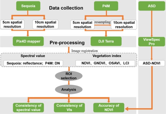
2.3. Data Collection

2.3.1. Sequoia and P4M Data

The UAV flight was conducted during sunny and clear sky (without clouds) conditions from 11:00 to 13:00 on 22 August 2019. During data collection, the Sequoia sensor was mounted on the EM6-800 hexarotor UAV, while the P4M was mounted on its own aircraft. For the Sequoia, a calibration target provided by the manufacturer was recorded to perform radiometric calibration in postprocessing.
In this experiment, the two sensors acquired a total of three sets of image data. The Sequoia images were collected while flying at 56 m height with 5 cm resolution and 100 m height with 10 cm resolution. The P4M images were collected while flying at 100 m height with 5 cm resolution. All of those flights were started within a one-hour period (11:27 to 12:22) to maintain similar illumination among each set of images. These images were acquired with 80% overlap. Sequoia acquired a total of 1715 images and P4M acquired 960 images. The specific parameter settings for the sensors are shown in Table 2.

2.3.2. ASD Data

We used the FieldSpec HandHeld 2 field spectroradiometer produced by Analytical Spectral Devices to measure the ground object spectral data. The coordinates and photos of the measured points were collected for ground object identification and visual interpretation of images. The spectroradiometer can perform continuous spectrum measurement in the wavelength range of 325–1075 nm, with the spectral resolution <3.0 nm at 700 nm, wavelength accuracy of ±1 nm, and field angle of 25°. It can measure the reflection, transmission, radiance, or irradiance in real time and obtain the continuous spectral curve of the measured object. The spectrum measurement was carried out in sunny and cloudless weather and the time was between 11:00 to 13:00. During the UAV flight, synchronous ground observation was carried out to ensure that the solar elevation angle, zenith angle, and weather conditions measured by the ground object spectrum were consistent with the UAV data. During data collection, the surveyors wore black clothing to absorb sunlight and reduce spectral interference. The spectrum measurement was carried out under natural light conditions, the spectroradiometer was held vertically downward at 1 m above the ground, and the sensor covered about 0.68 m2 ground area. To improve the accuracy of measurement, each ground point was repeatedly measured (ten times), and then the average value was taken. The spectroradiometer was calibrated every 10 min to reduce the interference of weather change on the spectrum measurement. Considering the small area, similar vegetation species, and relatively uniform ground surface in the study area, a total of eight ground points were selected (Figure 1). These points were selected randomly. Finally, according to Equation (1), the radiance of the ground object was converted into reflectance using the calibration coefficient provided by the reference plate.
R i = λ i m i n λ i m a x R λ C λ d λ λ i m i n λ i m a x C λ d λ
where R i is the reflectance of band i ( i = 1, 2, 3, 4), λ i m a x and λ i m i n are the maximum and minimum values of wavelength i , C λ is the transmittance of wavelength, and R λ is the reflectance of wavelength λ .
The reflectance data can be used to calculate the true NDVI of the ground point (ASD-NDVI). The area of each ground point is about 0.68 m2. Therefore, when comparing the NDVI obtained by the two sensors with the true NDVI (ASD-NDVI), 272 pixels were selected and the average NDVI was taken from the 5 cm resolution image. Similarly, when comparing the NDVI obtained by the two sensors with the true NDVI (ASD-NDVI), 68 pixels were selected and the average NDVI was taken from the 10 cm resolution image.

2.3.3. GCP

Five ground control points (GCPs) were evenly established on the field using printed white crosses to ensure the overlap between the Sequoia and P4M imagery at different times (Figure 1). The GCP and ASD coordinates were measured with 0.025 m horizontal accuracy and 0.035 m vertical accuracy. A geodetic dual-frequency global navigation satellite system (GNSS) receiver was used in a rapid-static manner (approximately 4 min for each measurement) using the relative positioning approach from a master station located at a point with known coordinates.

2.4. Methodology

This research methodology involved data acquisition (Section 2.3), preprocessing (Section 2.4), VI selection (Section 2.4), ROI selection (Section 2.4), and analysis (Section 3). The details are described after methodology chart (Figure 4).

2.4.1. Image Resampling

To standardize the spatial resolution of images acquired by different sensors, it is necessary to resample images that are very suitable for experimental comparison [46]. In order to avoid the contingency of the experimental results and to ensure the maneuverability of the UAV flight process, we compared the images of Sequoia and P4M with different spatial resolutions (5 and 10 cm). Therefore, we used ENVI software to resample the P4M images with the spatial resolution of 5 cm to obtain images with the spatial resolution of 10 cm. The pixel aggregate method was adopted in the resampling process [47].

2.4.2. Image Preprocessing

For preprocessing, Sequoia and P4M images were imported into Pix4D mapper [48] and DJI Terra software, respectively. Different steps of initial processing were followed, including point cloud processing, 3D model construction, feature extraction, feature construction, and orthophoto generation. As the Sequoia images can be used to directly obtain the reflectance data of the study area after processing, the VIs were calculated using reflectance data from VI equations. As the P4M images can be used to directly obtain the VIs, there was no need to get reflectance data for these images. Then, the processed images were imported into ENVI software to clip, match, and select different ROIs in a single band for comparison.
Figure 5 shows the processed 5 cm spatial resolution image. From Figure 5, it can be seen that there is a slight difference between a and b. For example, the building in the bottom left corner appears white in the P4M image but red in Sequoia, the stones on the right are white in P4M but red in Sequoia, and some roads which are white in P4M are yellow in Sequoia. These differences may be caused by the saturation of the red band in the Sequoia sensor. There are also some small differences between c and d. The Sequoia-derived NDVI (Sequoia-NDVI) is greater than the P4M-derived NDVI (P4M-NDVI); the range of Sequoia-NDVI is −0.19 to 0.93, and the range of P4M-NDVI is −0.43 to 0.85. There are some errors of Sequoia-NDVI in the visual range: Some buildings in the bottom left corner have the NDVI of about 0.7 (yellow part), but the building does not correspond to such a large NDVI value in reality.
Figure 6 shows the processed 10 cm spatial resolution images of Sequoia. Compared with the 5 cm spatial resolution results, both the false color RGB images (Figure 5a) and NDVI products (Figure 5c) are different. In the 10 cm resolution RGB image, the red part of the building in the bottom left corner still exists, but it is significantly smaller than in the 5 cm resolution image; the stones on the right are shown in white instead of red, and the road is shown in white instead of yellow. The problem of red band saturation does not seem to be obvious in 10 cm resolution images. Similarly, the NDVI value of the building in the bottom left corner seems normal.

2.4.3. ROI Selection

For the comparison of different sensors, the most common method is to compare the spectrum information or VI of each corresponding band by statistical regression [49]. In this experiment, four commonly used VIs were compared between Sequoia and P4M. In the spectrum information comparison, the reflectance of Sequoia cannot be directly compared with the DN value of P4M, so we used linear regression to characterize the spectral difference of these two sensors. Additionally, eight ground points were also measured by ASD, but the number of points was too limited to establish a fitting relationship between the ASD and the sensor. Therefore, we compared the NDVI between ASD and sensor point by point. For this experiment, we selected some ROIs in the same location (between images of two sensors) and then compared the average value in each ROI [50]. The images of the study area were divided into 10 × 8 grids on average, and a ROI was selected from each grid. A total of 80 homogeneous ROIs (including vegetation and nonvegetation) were selected in the experiment. The selected ROIs were in flat terrain, properly sized, homogeneous, and almost identical (no other object features were included) [51]. The relation function between Sequoia and P4M was fitted using ordinary least square (OLS) regression. The goodness of fit was defined by the correlation coefficient (also written as R2) [52]. Root-mean-square error (RMSE) was used to measure the deviation degree between the Sequoia-NDVI or P4M-NDVI and ASD-NDVI, as shown in Equation (2).
RMSE = i n ( y i - y i ) 2 n
where y i is the ASD-NDVI, y i is the average Sequoia-NDVI or P4M-NDVI, and n is the total number of ground points ( n = 8).

2.4.4. VI Selection

VIs can reflect the growth status of vegetation. Different VIs may have certain differences in reflecting vegetation characteristics [53]. In vegetation studies, among all the possible existent VIs, NDVI, green normalized difference vegetation index (GNDVI), optimal soil-adjusted vegetation index (OSAVI), and leaf chlorophyll index (LCI) are commonly used. These four VIs were compared in this experiment, as shown in Table 3. NDVI is currently the most widely used VI in the world. In agriculture, NDVI is one of the most important tools for crop yield estimation, biomass estimation, and so on [54]. Using the unique response characteristics of vegetation in the near-infrared band, NDVI combines the spectral values of the red band and near-infrared band to quantitatively describe the vegetation coverage in the study area.
Compared with NDVI, GNDVI is more sensitive to the change in vegetation chlorophyll content [55]. It combines the spectral values of the green band and the near-infrared band. OSAVI can reduce the interference of soil and vegetation canopy [15]. It also combines the spectral values of the red band and the near-infrared band. LCI is a sensitive indicator of chlorophyll content in leaves and is less affected by scattering from the leaf surface and internal structure variation [56]. It combines the spectral values of the red band, red edge band, and the near-infrared band. Different VIs were selected so that their VI equations contained different bands (Figure 3).

3. Results

3.1. Consistency of Spectral Values

In order to get better experiment results, we compared the images with 5 and 10 cm spatial resolution using the scatter plots of the Sequoia and P4M spectral values for the approximately equivalent spectral bands (green, red, red edge, and near-infrared). In the experiment, Sequoia used the spectral reflectance and P4M used the DN value of the image.
In the first experiment (5 cm spatial resolution), the spectral values of Sequoia and P4M were highly correlated (Figure 7). The two sensors showed a high correlation in the approximately equivalent four bands, and the correlation coefficient of the fitting function was not less than 0.90. The two sensors had the highest correlation in the red band (R2 = 0.9709), followed by the green band (R2 = 0.9699) and the red edge band (R2 = 0.9208); the correlation for the near-infrared band was lower than those of the other three bands (R2 = 0.9042). It was seen that the spectral values of Sequoia and P4M had an excellent correlation in the green and red bands, and the R2 was greater than 0.96. Meanwhile, the correlation was low in the red edge and the near-infrared bands, and the R2 was slightly less than 0.92. Thus, these results showed that spectral values of these two sensors had a high correlation in the green and red bands and a low correlation in the red edge and near-infrared bands.
In the second experiment (10 cm spatial resolution), the spectral values of Sequoia and P4M were also well correlated (Figure 8). In the four bands of these sensors, the correlation coefficient of the fitting equation was not less than 0.91, showing a strong correlation. As seen in the 5 cm spatial resolution results, the two sensors had the highest correlation in the red band (R2 = 0.9793), followed by the green band (R2 = 0.9727) and the red edge band (R2 = 0.9436); the correlation for the near-infrared band was lower than those of the other three bands (R2 = 0.9199). The spectral values of Sequoia and P4M were highly correlated in the green and red bands, and the R2 was greater than 0.97. Similarly, the correlations between the two sensors in the red edge and the near-infrared bands were low, and the R2 was slightly less than 0.94. These results also showed that spectral values of these two sensors had a high correlation in the green and red bands and a weak correlation in the red edge and near-infrared bands.
In short, the spectral values of Sequoia and P4M were highly correlated in both the green and red bands (R2 > 0.96), but the correlation was slightly lower in the red edge and the near-infrared bands (R2 < 0.96). The correlation of spectral values for the two sensors at 10 cm spatial resolution was slightly higher than that of 5 cm. Thus, if we are interested in using both images at the same time, the 10 cm spatial resolution image may be the better choice. Although these two sensors were highly correlated, there was also a slight difference, which may be caused by a variety of mixing factors, including the difference in spectral response function (Figure 3). Among the compared bands, the center wavelength and the wave width of these two sensors were both close in the green and red bands. Although the center wavelength of these two sensors was close in the red edge band, there was a big difference in the wave width. In the near-infrared band, the center wavelength and the wave width of the two sensors were significantly different. This explains how the spectral values differ between Sequoia and P4M.

3.2. Consistency of VI Products

The VI products of Sequoia and P4M were highly correlated (Figure 9). Four VIs were compared in this paper, namely NDVI, GNDVI, OSAVI, and LCI, as shown in Figure 9. The results on the left were obtained with 5 cm spatial resolution image, and those on the right were obtained with 10 cm spatial resolution. The black dotted lines are the 1:1 reference lines, and the solid lines are the fitting functions of these sensor-derived VIs (using OLS regression).
Among the four VIs, NDVI had the highest correlation, followed by OSAVI, GNDVI, and LCI. In the comparison of 5 cm spatial resolution images, the correlation of NDVI was the highest (R2 = 0.9863), followed by OSAVI (R2 = 0.9859), while GNDVI and LCI were lower (GNDVI: R2 = 0.9595; LCI: R2 = 0.9516). In the comparison of 10 cm spatial resolution images, the correlation of NDVI was still the highest (R2 = 0.9842), followed by OSAVI (R2 = 0.9806), while GNDVI and LCI were lower (GNDVI: R2 = 0.9518; LCI: R2 = 0.9546).
Sequoia-NDVI had better result than P4M-NDVI (most of the scattered points were distributed above the 1:1 line, and a very small part of the scattered points were located on or below the 1:1 line). The legend in Figure 5 also shows that Sequoia-NDVI was slightly higher than P4M-NDVI; the fitting results of GNDVI and LCI were similar to NDVI, and there were also some differences. In both resolutions, Sequoia-GNDVI was higher than P4M-GNDVI (all scattered points were distributed above the 1:1 line), but the distributions of points were more dispersed than those of NDVI. The fitting result of OSAVI was different from those of the previous three indices. In both resolutions, Sequoia-OSAVI was only partially higher than P4M-OSAVI (the scattered points were evenly distributed above, below, and on the 1:1 line).
Table 4 shows Sequoia and P4M VI transformation functions derived by OLS regression of the data shown in Figure 9. The transformation functions for the 5 and 10 cm spatial resolution images are listed separately, where S represents the VI of Sequoia and P represents the VI of P4M. Both sensors had good consistency in those four indices.
NDVI, GNDVI, OSAVI, and LCI were used for different combinations of surface reflectivity, so their values were partly determined by the reflectance of the green, red, red edge, and near-infrared bands. There was a certain difference in the spectral response functions of the sensors, which led to slight differences between the VI products. Although users cannot directly obtain the reflectance from P4M image, they can still obtain high-quality VI products. It was seen that P4M, which integrates aircraft, cameras, and data processing software, optimizes the user’s experience and improves the working efficiency by providing good VI products.

3.3. Accuracy of NDVI

Both the Sequoia-NDVI and P4M-NDVI had high accuracy, not only with a small deviation from ASD-NDVI but also with a good correlation (Figure 10). Two sets of spatial resolution data (5 and 10 cm) are compared in Figure 10: the left part shows the fitting scattered points of Sequoia-NDVI and ASD-NDVI, while the right part shows the fitting scattered points of P4M-NDVI and ASD-NDVI (blue dots correspond to 5 cm resolution and orange triangles correspond to 10 cm resolution). The Sequoia-NDVI was highly consistent with ASD-NDVI, and the correlation was high. In the comparative study of 5 cm spatial resolution images, RMSE = 0.0622 and R2 = 0.8523; in 10 cm spatial resolution images, RMSE = 0.0684 ad R2 = 0.8497. Similar to Sequoia, P4M-NDVI was also highly consistent with ASD-NDVI, maintaining a good correlation. In the comparative study, RMSE = 0.0886 and R2 = 0.8785 for 5 cm spatial resolution images, while RMSE = 0.0842 and R2 = 0.8785 for 10 cm spatial resolution images. This indicates that both Sequoia and P4M can provide NDVI products with high accuracy. Furthermore there was no big difference between the VI products obtained from these sensors.

4. Discussion

4.1. Differences between Sequoia and P4M

Different sensors may have different spectral response functions [59], and such differences will cause systematic deviations in the spectral values of the images. The consistency of spectral values between the two sensors studied showed a clear difference in the near-infrared band (Figure 7 and Figure 8). The reason for this might be due to their different spectral response functions (Figure 3). Compared with the spectral response function of Sequoia, the spectral range of P4M in the near-infrared band was wider than that of Sequoia (Sequoia: 40 nm; P4M: 52 nm), and the positions of center wavelength in the near-infrared band were also different (Sequoia: 790 nm; P4M: 840 nm). The results also showed that there was some difference in the red edge band. Although the center wavelengths of these two sensors were close in the red edge band (Sequoia: 735 nm; P4M: 730 nm), there were big differences in the wave width (Sequoia: 10 nm; P4M: 32 nm). In contrast, the center wavelength and the wave width of these two sensors were both close in the green (Sequoia: 550 nm and 40 nm; P4M: 560 nm and 32 nm) and red bands (Sequoia: 660 nm and 40 nm; P4M: 650 nm and 32 nm). The different spectral response functions may explain the difference in the spectral values between Sequoia and P4M.
In addition, other factors such as the spectral reflection characteristics of the ground object, the nonuniformity of the ground surface, the observation time, and the solar elevation angle also increased the randomness and uncertainty of this systematic deviation [60,61,62]. In this experiment, the ground surface of the study area was uniform, and the observation time was similar for both sensors, as was the solar elevation angle. Therefore, the reason for the difference in spectral values was probably related to the reflection characteristics of ground target features. The spectral value of a single pixel may be influenced by both the spectral response function and the reflection characteristics of the target feature. Therefore, some objects in the image having high reflection characteristics in a specific spectral band may often be more affected by the difference in spectral response function.
The acquisition of the VI usually requires a series of conversion processes on the spectral values; thus, if there is a deviation in the spectral values, the VI may also be affected. In analysis of the consistency of the VIs between the two sensors, the four VI products of Sequoia and P4M were found to be highly correlated, but there were still some differences. These differences may have a great relationship with the differences in spectral values between the sensors. The reason for this difference in spectral values is also the same as explained above (due to spectral response function). Therefore, this difference between VIs may be caused by the spectral response function and the reflection characteristics of the target features. As we know, the VI is obtained by combining the spectral values of different bands, so using different combination methods of spectral values may also affect the quality of the VI.

4.2. Sensitivity of VIs to Spectral Deviation

The calculation of the VI involved spectral values of different spectral bands. NDVI, GNDVI, OSAVI, and LCI were compared in this study, and their calculation included the spectral values of red, green, red edge, and near-infrared bands. Therefore, small changes in the spectral values of each band may have a relatively big impact on the VI results. In addition, the band combination method may also change the sensitivity of the VI to small changes in the spectral values. The experimental results showed that although the spectral values of the Sequoia and P4M were significantly different in the near-infrared band, this difference did not show a significant impact on the VI products. The correlation coefficients of the VI products obtained by these two sensors were greater than 0.95. The NDVI products of the two sensors were also compared with the ASD-NDVI. The results showed that Sequoia-NDVI and P4M-NDVI both have high accuracy. The normalized calculation method of VI eliminated the influence of the difference in spectral values to a certain extent, thus reducing the sensitivity of the VI to such spectral deviations [63].
Poncet et al. [64] found that the error of VIs was correlated with different radiometric calibration methods. In this experiment, for Sequoia, we used a calibration target provided by the manufacturer to perform radiometric calibration in postprocessing. The calibration method might have affected the reflectance, which would have affected the VI.

4.3. Selection of Optimal Spatial Scale

The pixel is the smallest unit that constitutes the remote sensing digital image. It is an important symbol to reflect the features of the image and can be used to characterize the ground conditions in the study area. The pixel size determines the spatial resolution of a digital image and amount of information it can contain. After resampling from high spatial resolution to low resolution, the resultant image (low spatial resolution) will lose spectral information and spectral variation [65]. With the increase of remote sensing image scale, the spectral features of several different ground objects may appear simultaneously in a single pixel, resulting in the generation of a mixed pixel. At this time, the signal intensity of the ground object features in the pixel tends to be stable, and the pixel signals received by different sensors will tend to be similar.
The correlation between the spectral values of Sequoia and P4M in each band (green, red, red edge, and near-infrared) seemed to have a certain relationship with the image scale. When the image scale was small (5 cm), the correlation was low; when the image scale was large (10 cm), the correlation was high (Table 5). Fawcett et al. [66] found that the NDVI consistency of a multispectral sensor was similar at different spatial resolutions. Our results also show that the NDVI consistencies of Sequoia and P4M at 5 and 10 cm resolutions are similar (5 cm: R2 = 0.9863; 10 cm: R2 = 0.9863).

4.4. Limitations

The study was carried out on a single date in a single study area with uniform vegetation species; it would be better if different study areas with different vegetation species in different periods were used. When assessing the suitability of UAV sensors in determining VIs, it would be important to include agricultural land, preferably with different nutrient treatments or crop species. Thus, in the future, it would be better to include agricultural land with crop species while doing VI-related research. Similarly, to assess the accuracy of NDVI, eight ASD points were used, as the terrain was uniform; still, better results could be obtained if more points were used. The use of more than two multispectral minisensors could be more meaningful to analyze the consistency of spectral values, consistency of VI products, and accuracy of NDVI. Therefore, detailed research is needed in the future to obtain improved results and conclusions.

5. Conclusions

Different UAV multispectral minisensors have been developed for applications in various fields, but their experimental performance and consistency need to be determined before their application. As a preliminary work towards consistency evaluation, different UAV images from Sequoia and P4M sensors with multispectral bands were acquired and preprocessed for ROI creation and VI calculation. The main objective of this research was to experimentally evaluate different UAV multispectral minisensors and compare them in terms of consistency. Using a combined method of consistency of spectral values, consistency of VI products, and accuracy of NDVI, we came to the following conclusions: First, the data acquisition capability of the Sequoia is similar to that of the P4M; both the spectral values and VIs of the two sensors have good correlation (R2 > 0.90). Second, the VI products obtained from both sensors have good precision, and they are suitable for vegetation remote sensing monitoring. Third, both sensors have similar characteristics, and they may be used interchangeably for large area coverage with high spatial resolution and for daily time series science and applications.

Author Contributions

H.L., T.F., and L.D. designed and developed the research idea. H.Z. conducted the field data collection. H.L. and T.F. processed all remaining data. H.L. performed the data analysis and wrote the manuscript. H.L., T.F., P.G., and L.D. contributed to results and data interpretation, discussion, and revision of the manuscript. All the authors revised and approved the manuscript. All authors have read and agreed to the published version of the manuscript.

Funding

This research was funded by the National Key Research & Development Program of China (No. 2018YFC0706004).

Acknowledgments

The authors are very thankful for the valuable support of Zou Han Yue, Qiao Dan Yu, and Chen Yong.

Conflicts of Interest

The authors declare no conflict of interest. The funders had no role in the design of the study; in the collection, analyses, or interpretation of data; in the writing of the manuscript, or in the decision to publish the results.

References

  1. Berni, J.; Zarco-Tejada, P.J.; Suarez, L.; Fereres, E. Thermal and Narrowband Multispectral Remote Sensing for Vegetation Monitoring From an Unmanned Aerial Vehicle. IEEE T. Geosci. Remote. 2009, 47, 722–738. [Google Scholar] [CrossRef] [Green Version]
  2. Iizuka, K.; Itoh, M.; Shiodera, S.; Matsubara, T.; Dohar, M.; Watanabe, K. Advantages of unmanned aerial vehicle (UAV) photogrammetry for landscape analysis compared with satellite data: A case study of postmining sites in Indonesia. Cogent Geosci. 2018, 4, 1498180. [Google Scholar] [CrossRef]
  3. Matese, A.; Toscano, P.; Di Gennaro, S.; Genesio, L.; Vaccari, F.; Primicerio, J.; Belli, C.; Zaldei, A.; Bianconi, R.; Gioli, B. Intercomparison of UAV, Aircraft and Satellite Remote Sensing Platforms for Precision Viticulture. Remote Sens. 2015, 7, 2971–2990. [Google Scholar] [CrossRef] [Green Version]
  4. Kelcey, J.; Lucieer, A. Sensor Correction And Radiometric Calibration Of A 6-Band Multispectral Imaging Sensor For Uav Remote Sensing. ISPRS—Int. Arch. Photogramm. Remote Sens. Spat. Inf. Sci. 2012, XXXIX-B1, 393–398. [Google Scholar] [CrossRef] [Green Version]
  5. Dash, J.P.; Watt, M.S.; Pearse, G.D.; Heaphy, M.; Dungey, H.S. Assessing very high resolution UAV imagery for monitoring forest health during a simulated disease outbreak. ISPRS J. Photogramm. 2017, 131, 1–14. [Google Scholar] [CrossRef]
  6. Lu, B.; He, Y. Species classification using Unmanned Aerial Vehicle (UAV)-acquired high spatial resolution imagery in a heterogeneous grassland. ISPRS J. Photogramm. 2017, 128, 73–85. [Google Scholar] [CrossRef]
  7. Puliti, S.; Ene, L.T.; Gobakken, T.; Næsset, E. Use of partial-coverage UAV data in sampling for large scale forest inventories. Remote Sens. Environ. 2017, 194, 115–126. [Google Scholar] [CrossRef]
  8. Bendig, J.; Yu, K.; Aasen, H.; Bolten, A.; Bennertz, S.; Broscheit, J.; Gnyp, M.L.; Bareth, G. Combining UAV-based plant height from crop surface models, visible, and near infrared vegetation indices for biomass monitoring in barley. Int. J. Appl. Earth Obs. 2015, 39, 79–87. [Google Scholar] [CrossRef]
  9. Candiago, S.; Remondino, F.; De Giglio, M.; Dubbini, M.; Gattelli, M. Evaluating Multispectral Images and Vegetation Indices for Precision Farming Applications from UAV Images. Remote Sens. 2015, 7, 4026–4047. [Google Scholar] [CrossRef] [Green Version]
  10. Feng, Q.; Liu, J.; Gong, J. UAV Remote Sensing for Urban Vegetation Mapping Using Random Forest and Texture Analysis. Remote Sens. 2015, 7, 1074–1094. [Google Scholar] [CrossRef] [Green Version]
  11. Kamble, B.; Kilic, A.; Hubbard, K. Estimating Crop Coefficients Using Remote Sensing-Based Vegetation Index. Remote Sens. 2013, 5, 1588–1602. [Google Scholar] [CrossRef] [Green Version]
  12. Liu, J.; Pattey, E.; Jégo, G. Assessment of vegetation indices for regional crop green LAI estimation from Landsat images over multiple growing seasons. Remote Sens. Environ. 2012, 123, 347–358. [Google Scholar] [CrossRef]
  13. Motohka, T.; Nasahara, K.N.; Oguma, H.; Tsuchida, S. Applicability of Green-Red Vegetation Index for Remote Sensing of Vegetation Phenology. Remote Sens. 2010, 2, 2369–2387. [Google Scholar] [CrossRef] [Green Version]
  14. Lunetta, R.S.; Knight, J.F.; Ediriwickrema, J.; Lyon, J.G.; Worthy, L.D. Land-cover change detection using multi-temporal MODIS NDVI data. Remote Sens. Environ. 2006, 105, 142–154. [Google Scholar] [CrossRef]
  15. Huete, A.R. A soil-adjusted vegetation index (SAVI). Remote Sens. Environ. 1988, 25, 295–309. [Google Scholar] [CrossRef]
  16. Ye, H.; Huang, W.; Huang, S.; Cui, B.; Dong, Y.; Guo, A.; Ren, Y.; Jin, Y. Recognition of Banana Fusarium Wilt Based on UAV Remote Sensing. Remote Sens. 2020, 12, 938. [Google Scholar] [CrossRef] [Green Version]
  17. Ashapure, A.; Jung, J.; Chang, A.; Oh, S.; Maeda, M.; Landivar, J. A Comparative Study of RGB and Multispectral Sensor-Based Cotton Canopy Cover Modelling Using Multi-Temporal UAS Data. Remote Sens. 2019, 11, 2757. [Google Scholar] [CrossRef] [Green Version]
  18. Iizuka, K.; Kato, T.; Silsigia, S.; Soufiningrum, A.Y.; Kozan, O. Estimating and Examining the Sensitivity of Different Vegetation Indices to Fractions of Vegetation Cover at Different Scaling Grids for Early Stage Acacia Plantation Forests Using a Fixed-Wing UAS. Remote Sens. 2019, 11, 1816. [Google Scholar] [CrossRef] [Green Version]
  19. Lima-Cueto, F.J.; Blanco-Sepúlveda, R.; Gómez-Moreno, M.L.; Galacho-Jiménez, F.B. Using Vegetation Indices and a UAV Imaging Platform to Quantify the Density of Vegetation Ground Cover in Olive Groves (Olea Europaea L.) in Southern Spain. Remote Sens. 2019, 11, 2564. [Google Scholar] [CrossRef] [Green Version]
  20. Freeman, D.; Gupta, S.; Smith, D.H.; Maja, J.M.; Robbins, J.; Owen, J.S.; Peña, J.M.; de Castro, A.I. Watson on the Farm: Using Cloud-Based Artificial Intelligence to Identify Early Indicators of Water Stress. Remote Sens. 2019, 11, 2645. [Google Scholar] [CrossRef] [Green Version]
  21. Dash, J.; Pearse, G.; Watt, M. UAV Multispectral Imagery Can Complement Satellite Data for Monitoring Forest Health. Remote Sens. 2018, 10, 1216. [Google Scholar] [CrossRef] [Green Version]
  22. Albetis, J.; Duthoit, S.; Guttler, F.; Jacquin, A.; Goulard, M.; Poilvé, H.; Féret, J.; Dedieu, G. Detection of Flavescence dorée Grapevine Disease Using Unmanned Aerial Vehicle (UAV) Multispectral Imagery. Remote Sens. 2017, 9, 308. [Google Scholar] [CrossRef] [Green Version]
  23. Gevaert, C.M.; Suomalainen, J.; Tang, J.; Kooistra, L. Generation of Spectral–Temporal Response Surfaces by Combining Multispectral Satellite and Hyperspectral UAV Imagery for Precision Agriculture Applications. IEEE J.-Stars. 2015, 8, 3140–3146. [Google Scholar] [CrossRef]
  24. Suárez, L.; Zarco-Tejada, P.J.; Berni, J.A.J.; González-Dugo, V.; Fereres, E. Modelling PRI for water stress detection using radiative transfer models. Remote Sens. Environ. 2009, 113, 730–744. [Google Scholar] [CrossRef] [Green Version]
  25. Ahmed, O.S.; Shemrock, A.; Chabot, D.; Dillon, C.; Williams, G.; Wasson, R.; Franklin, S.E. Hierarchical land cover and vegetation classification using multispectral data acquired from an unmanned aerial vehicle. Int. J Remote Sens. Unmanned Aer. Veh. Environ. Appl. 2017, 38, 2037–2052. [Google Scholar] [CrossRef]
  26. Ke, Y.; Im, J.; Lee, J.; Gong, H.; Ryu, Y. Characteristics of Landsat 8 OLI-derived NDVI by comparison with multiple satellite sensors and in-situ observations. Remote Sens. Environ. 2015, 164, 298–313. [Google Scholar] [CrossRef]
  27. Cheng, Y.; Gamon, J.; Fuentes, D.; Mao, Z.; Sims, D.; Qiu, H.; Claudio, H.; Huete, A.; Rahman, A. A multi-scale analysis of dynamic optical signals in a Southern California chaparral ecosystem: A comparison of field, AVIRIS and MODIS data. Remote Sens. Environ. 2006, 103, 369–378. [Google Scholar] [CrossRef]
  28. Soudani, K.; François, C.; le Maire, G.; Le Dantec, V.; Dufrêne, E. Comparative analysis of IKONOS, SPOT, and ETM+ data for leaf area index estimation in temperate coniferous and deciduous forest stands. Remote Sens. Environ. 2006, 102, 161–175. [Google Scholar] [CrossRef] [Green Version]
  29. Goward, S.N.; Davis, P.E.; Fleming, D.; Miller, L.; Townshend, J.R. Empirical comparison of Landsat 7 and IKONOS multispectral measurements for selected Earth Observation System (EOS) validation sites. Remote Sens. Environ. 2003, 88, 80–99. [Google Scholar] [CrossRef]
  30. Zhang, H.K.; Roy, D.P.; Yan, L.; Li, Z.; Huang, H.; Vermote, E.; Skakun, S.; Roger, J. Characterization of Sentinel-2A and Landsat-8 top of atmosphere, surface, and nadir BRDF adjusted reflectance and NDVI differences. Remote Sens. Environ. 2018, 215, 482–494. [Google Scholar] [CrossRef]
  31. Ahmadian, N.; Ghasemi, S.; Wigneron, J.; Zölitz, R. Comprehensive study of the biophysical parameters of agricultural crops based on assessing Landsat 8 OLI and Landsat 7 ETM+ vegetation indices. Gisci. Remote Sens. 2016, 53, 337–359. [Google Scholar] [CrossRef]
  32. Roy, D.P.; Kovalskyy, V.; Zhang, H.K.; Vermote, E.F.; Yan, L.; Kumar, S.S.; Egorov, A. Characterization of Landsat-7 to Landsat-8 reflective wavelength and normalized difference vegetation index continuity. Remote Sens. Environ. 2016, 185, 57–70. [Google Scholar] [CrossRef] [PubMed] [Green Version]
  33. Phongaksorn, N.; Tripathi, N.K.; Kumar, S.; Soni, P. Inter-Sensor Comparison between THEOS and Landsat 5 TM Data in a Study of Two Crops Related to Biofuel in Thailand. Remote Sens. 2012, 4, 354–376. [Google Scholar] [CrossRef] [Green Version]
  34. Runge, A.; Grosse, G. Comparing Spectral Characteristics of Landsat-8 and Sentinel-2 Same-Day Data for Arctic-Boreal Regions. Remote Sens. 2019, 11, 1730. [Google Scholar] [CrossRef] [Green Version]
  35. Chastain, R.; Housman, I.; Goldstein, J.; Finco, M.; Tenneson, K. Empirical cross sensor comparison of Sentinel-2A and 2B MSI, Landsat-8 OLI, and Landsat-7 ETM+ top of atmosphere spectral characteristics over the conterminous United States. Remote Sens. Environ. 2019, 221, 274–285. [Google Scholar] [CrossRef]
  36. Flood, N. Comparing Sentinel-2A and Landsat 7 and 8 using surface reflectance over Australia. Remote Sens. 2017, 9, 659. [Google Scholar] [CrossRef] [Green Version]
  37. Mandanici, E.; Bitelli, G. Preliminary comparison of sentinel-2 and landsat 8 imagery for a combined use. Remote Sens. 2016, 8, 1014. [Google Scholar] [CrossRef] [Green Version]
  38. Claverie, M.; Vermote, E.F.; Franch, B.; Masek, J.G. Evaluation of the Landsat-5 TM and Landsat-7 ETM+ surface reflectance products. Remote Sens. Environ. 2015, 169, 390–403. [Google Scholar] [CrossRef]
  39. von Bueren, S.K.; Burkart, A.; Hueni, A.; Rascher, U.; Tuohy, M.P.; Yule, I. Deploying four optical UAV-based sensors over grassland: Challenges and limitations. Biogeosciences 2015, 12, 163–175. [Google Scholar] [CrossRef] [Green Version]
  40. Bareth, G.; Aasen, H.; Bendig, J.; Gnyp, M.L.; Bolten, A.; Jung, A.; Michels, R.; Soukkamäki, J. Low-weight and UAV-based hyperspectral full-frame cameras for monitoring crops: Spectral comparison with portable spectroradiometer measurements. Photogramm.-Fernerkund.-Geoinf. 2015, 2015, 69–79. [Google Scholar] [CrossRef]
  41. Nebiker, S.; Lack, N.; Abächerli, M.; Läderach, S. Light-weight multispectral UAV sensors and their capabilities for predicting grain yield and detecting plant diseases. Int. Arch. Photogramm. Remote Sens. Spat. Inf. Sci. 2016, 41. [Google Scholar] [CrossRef] [Green Version]
  42. Deng, L.; Mao, Z.; Li, X.; Hu, Z.; Duan, F.; Yan, Y. UAV-based multispectral remote sensing for precision agriculture: A comparison between different cameras. ISPRS J. Photogramm. 2018, 146, 124–136. [Google Scholar] [CrossRef]
  43. Parrot. Available online: https://support.parrot.com/us/support/products/parrot-sequoia (accessed on 23 July 2020).
  44. P4 Multispectral. Available online: https://www.dji.com/nl/p4-multispectral?site=brandsite&from=nav (accessed on 23 July 2020).
  45. EM6-800. Available online: http://www.easydrone.com.cn (accessed on 23 July 2020).
  46. Gurjar, S.B.; Padmanabhan, N. Study of various resampling techniques for high-resolution remote sensing imagery. J. Indian Soc. Remote. 2005, 33, 113–120. [Google Scholar] [CrossRef]
  47. Keys, R. Cubic convolution interpolation for digital image processing. IEEE Trans. Acoust. Speech Signal Process. 1981, 29, 1153–1160. [Google Scholar] [CrossRef] [Green Version]
  48. Allred, B.; Eash, N.; Freeland, R.; Martinez, L.; Wishart, D. Effective and efficient agricultural drainage pipe mapping with UAS thermal infrared imagery: A case study. Agr. Water Manag. 2018, 197, 132–137. [Google Scholar] [CrossRef]
  49. Xu, H.; Zhang, T. Assessment of consistency in forest-dominated vegetation observations between ASTER and Landsat ETM+ images in subtropical coastal areas of southeastern China. Agr. For. Meteorol. 2013, 168, 1–9. [Google Scholar] [CrossRef]
  50. Saunier, S.; Goryl, P.; Chander, G.; Santer, R.; Bouvet, M.; Collet, B.; Mambimba, A.; Kocaman Aksakal, S. Radiometric, Geometric, and Image Quality Assessment of ALOS AVNIR-2 and PRISM Sensors. IEEE T. Geosci. Remote. 2010, 48, 3855–3866. [Google Scholar] [CrossRef]
  51. Xiao-ping, W.; Han-qiu, X. Cross-Comparison between GF-2 PMS2 and ZY-3 MUX Sensor Data. Spectrosc. Spect. Anal. 2019, 39, 310–318. [Google Scholar]
  52. Halliday, M.A.K.; Hasan, R. Cohesion in English; Taylor & Francis: New York, NY, USA, 2014. [Google Scholar]
  53. Boyte, S.P.; Wylie, B.K.; Rigge, M.B.; Dahal, D. Fusing MODIS with Landsat 8 data to downscale weekly normalized difference vegetation index estimates for central Great Basin rangelands, USA. Gisci. Remote Sens. 2017, 55, 376–399. [Google Scholar] [CrossRef]
  54. Rouse, J.W., Jr.; Haas, R.H.; Schell, J.A.; Deering, D.W. Monitoring Vegetation Systems in the Great Plains with Erts; Nasa Special Publication: Washington, DC, USA, 1973; pp. 309–317.
  55. Gitelson, A.A.; Kaufman, Y.J.; Merzlyak, M.N. Use of a green channel in remote sensing of global vegetation from EOS-MODIS. Remote Sens. Environ. 1996, 58, 289–298. [Google Scholar] [CrossRef]
  56. Pu, R.; Gong, P.; Yu, Q. Comparative analysis of EO-1 ALI and Hyperion, and Landsat ETM+ data for mapping forest crown closure and leaf area index. Sensors 2008, 8, 3744–3766. [Google Scholar] [CrossRef] [Green Version]
  57. Haboudane, D. Hyperspectral vegetation indices and novel algorithms for predicting green LAI of crop canopies: Modeling and validation in the context of precision agriculture. Remote Sens. Environ. 2004, 90, 337–352. [Google Scholar] [CrossRef]
  58. Zarco-Tejada, P.J.; Miller, J.R.; Morales, A.; Berjón, A.; Agüera, J. Hyperspectral indices and model simulation for chlorophyll estimation in open-canopy tree crops. Remote Sens. Environ. 2004, 90, 463–476. [Google Scholar] [CrossRef]
  59. Ghimire, P.; Lei, D.; Juan, N. Effect of Image Fusion on Vegetation Index Quality—A Comparative Study from Gaofen-1, Gaofen-2, Gaofen-4, Landsat-8 OLI and MODIS Imagery. Remote Sens. 2020, 12, 1550. [Google Scholar] [CrossRef]
  60. Flood, N. Continuity of reflectance data between Landsat-7 ETM+ and Landsat-8 OLI, for both top-of-atmosphere and surface reflectance: A study in the Australian landscape. Remote Sens. 2014, 6, 7952–7970. [Google Scholar] [CrossRef] [Green Version]
  61. Barsi, J.A.; Lee, K.; Kvaran, G.; Markham, B.L.; Pedelty, J.A. The spectral response of the Landsat-8 operational land imager. Remote Sens. 2014, 6, 10232–10251. [Google Scholar] [CrossRef] [Green Version]
  62. Wang, Z.; Coburn, C.A.; Ren, X.; Teillet, P.M. Effect of soil surface roughness and scene components on soil surface bidirectional reflectance factor. Can. J. Soil Sci. 2012, 92, 297–313. [Google Scholar] [CrossRef]
  63. Wang, Z.; Liu, C.; Huete, A. From AVHRR-NDVI to MODIS-EVI: Advances in vegetation index research. Acta Ecol. Sin. 2003, 23, 979–987. [Google Scholar]
  64. Poncet, A.M.; Knappenberger, T.; Brodbeck, C.; Fogle, M.; Shaw, J.N.; Ortiz, B.V. Multispectral UAS data accuracy for different radiometric calibration methods. Remote Sens. 2019, 11, 1917. [Google Scholar] [CrossRef] [Green Version]
  65. Woodcock, C.E.; Strahler, A.H. The factor of scale in remote sensing. Remote Sens. Environ. 1987, 21, 311–332. [Google Scholar] [CrossRef]
  66. Fawcett, D.; Panigada, C.; Tagliabue, G.; Boschetti, M.; Celesti, M.; Evdokimov, A.; Biriukova, K.; Colombo, R.; Miglietta, F.; Rascher, U. Multi-Scale Evaluation of Drone-Based Multispectral Surface Reflectance and Vegetation Indices in Operational Conditions. Remote Sens. 2020, 12, 514. [Google Scholar] [CrossRef] [Green Version]
Figure 1. Location of study area.
Remotesensing 12 02542 g001
Figure 2. UAV platforms and multispectral sensors (Sequoia and P4M). The Sequoia sensor is carried on the EM6-800 hexarotor UAV (left), and the P4M uses its own aircraft (right).
Remotesensing 12 02542 g002
Figure 3. Spectral response functions of Sequoia (solid lines) and P4M (dashed lines).
Remotesensing 12 02542 g003
Figure 4. Methodological flowchart of the research.
Remotesensing 12 02542 g004
Figure 5. Image pairs of Sequoia and P4M (5 cm) after data processing: (a,b) two false color composites formed by the combination of near-infrared, red, and green bands; (c,d) normalized difference vegetation index (NDVI) products of the two sensors. The left side corresponds to the Sequoia camera, and the right side corresponds to the P4M camera. The yellow squares indicate the difference between Sequoia-derived RGB and P4M-derived RGB; the black squares indicate the difference between Sequoia-NDVI and P4M-NDVI.
Remotesensing 12 02542 g005
Figure 6. Image pairs of Sequoia (10 cm) after data processing: (a) the false color composite formed by the combination of near-infrared, red, and green bands; (b) normalized difference vegetation index (NDVI) product of Sequoia.
Remotesensing 12 02542 g006
Figure 7. Scatter plots of Sequoia and P4M spectral values (5 cm) in the green band (a), red band (b), red edge band (c) and near infrared band (d). The solid lines show OLS regression of the Sequoia and the P4M data, and the dotted lines are 1:1 lines for reference.
Remotesensing 12 02542 g007
Figure 8. Scatter plots of Sequoia and P4M spectral values (10 cm) in the green band (a), red band (b), red edge band (c) and near infrared band (d).
Remotesensing 12 02542 g008
Figure 9. Scatter plots of Sequoia and P4M vegetation indices, which corresponded to the NDVI, GNDVI, OSAVI and LCI with 5cm spatial resolution (a, c, e and g) and 10cm (b, d, f and h).
Remotesensing 12 02542 g009
Figure 10. Scatter plots of Sequoia-NDVI (a) and P4M-NDVI (b) with ASD-NDVI. The blue dotted lines show OLS regression of Sequoia-NDVI (P4M-NDVI) and ASD-NDVI data with 5 cm resolution. The orange dotted lines show OLS regression of Sequoia-NDVI (P4M-NDVI) and ASD-NDVI data with 10 cm resolution.
Remotesensing 12 02542 g010
Table 1. Spectral band information for the Parrot Sequoia (Sequoia) and DJI Phantom 4 Multispectral (P4M). Their approximately equivalent bands (green, red, red edge, and near-infrared) were compared in this study.
Sequoia P4M
BandCentral Wavelength (nm)Wavelength Width (nm)BandCentral Wavelength (nm)Wavelength Width (nm)
---blue45032
green55040green56032
red66040red65032
red edge73510red edge73032
near-infrared79040near-infrared84052
Table 2. Parameters of sensors used for comparison. During the data collection process, the P4M camera failed to successfully acquire image data with a resolution of 10 cm. The 10 cm image data used in the comparative experiment was obtained by resampling the 5 cm image.
SensorDateTimeAltitude (m)Solar Zenith (°)Solar Azimuth (°)Resolution (m)
P4M2019.8.2211:2710029.8031155.000.05
Sequoia2019.8.2211:595627.9838170.800.05
Sequoia2019.8.2212:2210027.7342182.630.10
Table 3. Four vegetation indices (VIs) used for the research.
VIFormulaReference
Normalized Difference Vegetation Index(NIR − R)/(NIR + R)[57]
Green Normalized Difference Vegetation Index(NIR − G)/(NIR + G)[55]
Optimal Soil-Adjusted Vegetation Index(NIR − R)/(NIR + R + 0.16)[58]
Leaf Chlorophyll Index(NIR − RE)/(NIR + R)[56]
NIR, R, G, RE: Reflectance of near-infrared, red, green, and red edge bands.
Table 4. Sequoia and P4M VI transformation functions derived by OLS regression of the data illustrated in Figure 9.
5 cm 10 cm
VIsNFunctionR2FunctionR2
NDVI80S = 1.1211 × P + 0.05790.9863S = 1.1234 × P + 0.06450.9842
GNDVI80S = 0.9693 × P + 0.15990.9595S = 0.9721 × P + 0.16120.9518
OSAVI80S = 0.8322 × P + 0.04440.9859S = 0.8182 × P + 0.05280.9806
LCI80S = 0.8221 × P + 0.05960.9516S = 0.8330 × P + 0.05890.9546
S: Sequoia, P: P4M.
Table 5. Sequoia and P4M spectral value transformation functions and the values of their correlation coefficients (R2).
5 cm 10 cm
BandFunctionR2FunctionR2
greenS = 0.8869 × P − 0.01110.9699S = 0.9242 × P − 0.01540.9727
redS = 1.1867 × P − 0.03550.9709S = 1.2294 × P − 0.03900.9793
red edgeS = 0.9868 × P + 0.03590.9208S = 1.0345 × P + 0.02370.9436
near-infraredS = 0.7468 × P + 0.03390.9042S = 1.2405 × P − 0.01590.9199
S: Sequoia, P: P4M.

