Assessing Typhoon-Induced Canopy Damage Using Vegetation Indices in the Fushan Experimental Forest, Taiwan

Abstract

Cyclonic windstorms profoundly affect forest structure and function throughout the tropics and subtropics. Remote sensing techniques and vegetation indices (VIs) have improved our ability to characterize cyclone impacts over broad spatial scales. Although VIs are useful for understanding changes in forest cover, their consistency on detecting changes in vegetation cover is not well understood. A better understanding of the similarities and differences in commonly used VIs across disturbance events and forest types is needed to reconcile the results from different studies. Using Landsat imagery, we analyzed the change between pre- and post-typhoon VI values (ΔVIs) of four VIs for five typhoons (local name of cyclones in the North Pacific) that affected the Fushan Experimental Forest of Taiwan. We found that typhoons varied in their effect on forest canopy cover even when they had comparable trajectories, wind speeds, and rainfall. Most VIs measured a decrease in forest cover following typhoons, ranging from −1.18% to −19.87%; however, the direction of ΔVI–topography relationships varied among events. All typhoons significantly increased vegetation heterogeneity, and ΔVI was negatively related to pre-typhoon VI across all typhoons. Four of the five typhoons showed that more frequently affected sites had greater VI decreases. VIs ranged in their sensitivity to detect typhoon-induced changes in canopy coverage, and no single VI was most sensitive across all typhoons. Therefore, we recommend using VIs in combination—for example Normalized Difference Infrared Index (NDII) and Enhanced Vegetation Index (EVI), when comparing cyclone-disturbance-induced changes in vegetation cover among disturbances and across forests.

1. Introduction

Tropical forests harbor a large portion of global biodiversity [1] and play a key role in global carbon cycling [2,3,4]. An estimated 52% of the terrestrial carbon pool is contained by tropical and subtropical forests, although they cover less than 15% of the land surfaces excluding Antarctica [5]. Thus, changes in the geographic extent and quality (i.e., structure) of tropical forests have major effects on biodiversity conservation efforts [6,7] and important ecological processes such as carbon sequestration [8,9]. Disturbances such as fires, pathogens, and tropical cyclones are important agents affecting the dynamics of many tropical and subtropical forests [10,11,12]. Tropical cyclones are among the most common natural disturbances to tropical and subtropical forests [13]. Cyclones vary in their effects on forest structure and damage to individual trees, with damage ranging from defoliation and branch-stripping to bole-snapping and the uprooting of trees [14]. These events have consequences for forest functioning through the changing of canopy cover, gap formation, and tree population demography [12,15].

Spatial patterns of damage are key to understanding forest ecosystem dynamics in relation to cyclone disturbance at the landscape scale. In addition to vegetation characteristics such as forest type, species, phenological and successional state [16,17,18,19,20,21,22], and the distance to cyclone eye [23,24,25,26], landscape topography is also a main factor which modulates cyclone disturbance effects on vegetation [27,28]. Cyclones tend to have greater effects in exposed areas, such as ridges or windward slopes [25,26,29,30,31,32,33]. In addition, cyclone damages may vary with elevation [31,34], slope steepness [20,32] and topographic position [18,20,29,32]. The interactions among the topographical variables, biotic characteristics, and wind properties lead to complex patterns of cyclone effects across the landscape [25,32,35,36]. Thus, the spatial patterns of cyclone effects are likely to vary among different cyclone events. In fact, dissimilarities in ecological effects among multiple cyclones have been reported for various sites, including when several typhoons (local name of tropical cyclones in the Northwest Pacific) have occurred in a short time period with similar tracks [21,25,37,38,39]. Because topographical characteristics are key to cyclone effects, to better predict cyclone effects on forest landscapes it is important to examine which topographic properties have consistent relationships with cyclone disturbance and which ones are more variable. Few studies have compared landscape damage patterns of multiple cyclones [36,40], possibly due to the scarcity of cyclones over a period of time during which the changes in vegetation patterns are minimal except for those caused by cyclones in most regions.

Cyclone effects on vegetation can be assessed through direct field observations (e.g., [16,41,42]) or the use of remote sensing techniques (e.g., [23,32,43]). Remote sensing offers the possibility of assessment of cyclone effects over broad areas [23,32,44], and the results have been used to formulate conservation recommendations [45,46,47]. Used in combination with other data, remote sensing can effectively identify broad spatial patterns of cyclone damage in relation to vegetation types and topographical properties [20,32,43,47] that could be otherwise difficult to assess with ground surveys. Some of the most commonly used remote sensing data are vegetation indices (VIs), which are derived from satellite or aircraft-collected spectral reflectance measurements.

Many VIs have been developed to assess landscape vegetation patterns and dynamics [48], with each having its strengths and weaknesses [49]. VIs based on measurements using near-infrared (NIR) spectral bands, such as the Enhanced Vegetation Index (EVI), the Normalized Difference Vegetation Index (NDVI), and the Soil-Adjusted Vegetation Index (SAVI), have been widely used in vegetation assessments [48,50,51,52] although the shortwave infrared band of Landsat has also been shown to be effective for evaluating photosynthesis and forest canopy cover [53,54]. Relationships between VIs and forest characteristics are diverse and can be context-dependent; however, generally, the EVI is more closely related to canopy structure [55] and has a better relationship with photosynthesis than NDVI under high leaf area index (LAI, [56]) because EVI is less likely to saturate than NDVI at high vegetation cover [57,58,59]. The Normalized Difference Infrared Index (NDII), another NIR-based index, has been shown to be more sensitive than the NDVI to changes in vegetation water content [60], particularly at high vegetation cover [61,62]. The SAVI, also an NIR-based index, could be an option when the influence from exposed soil is a concern, such as in disturbed areas with low vegetation cover [63]. Disparate uses of VIs in studies of forest disturbances make cross-study comparisons difficult. Hence, a better comprehension of the comparability among frequently used VIs (i.e., NDVI, EVI, NDII) in relation to forest disturbance and recovery is needed for studies of vegetation disturbance ecology using VIs. Given the widespread occurrence and frequency of cyclones, they provide an opportunity to comparatively evaluate the effectiveness and consistency of VIs to capture vegetation disturbance and recovery within and across cyclones and forests.

The Fushan Experimental Forest (FEF) in north-eastern Taiwan provides a unique opportunity to study and compare the effects of multiple typhoons, as it was hit by nearly one typhoon per year between 1951 and 2005, including many years with multiple typhoons of different trajectories [42,64,65]. The frequent typhoon occurrence in this site has permitted the study of disturbance representativeness of large forest plots over a wider landscape [66], but understanding of damage variation and the comparability of different VIs across typhoons is lacking. Here, taking advantage of the FEF location, we use remotely sensed data to examine: (1) the consistency of patterns of typhoon damages among different typhoons; (2) the spatial patterns of typhoon damage in relation to cyclone properties (i.e., wind direction) and site topographical features (e.g., elevation, slope, and aspect); (3) the relationships between typhoon frequency and severity of typhoon damage; and (4) whether patterns of typhoon damage are consistent among different vegetation indices.

2. Materials and Methods

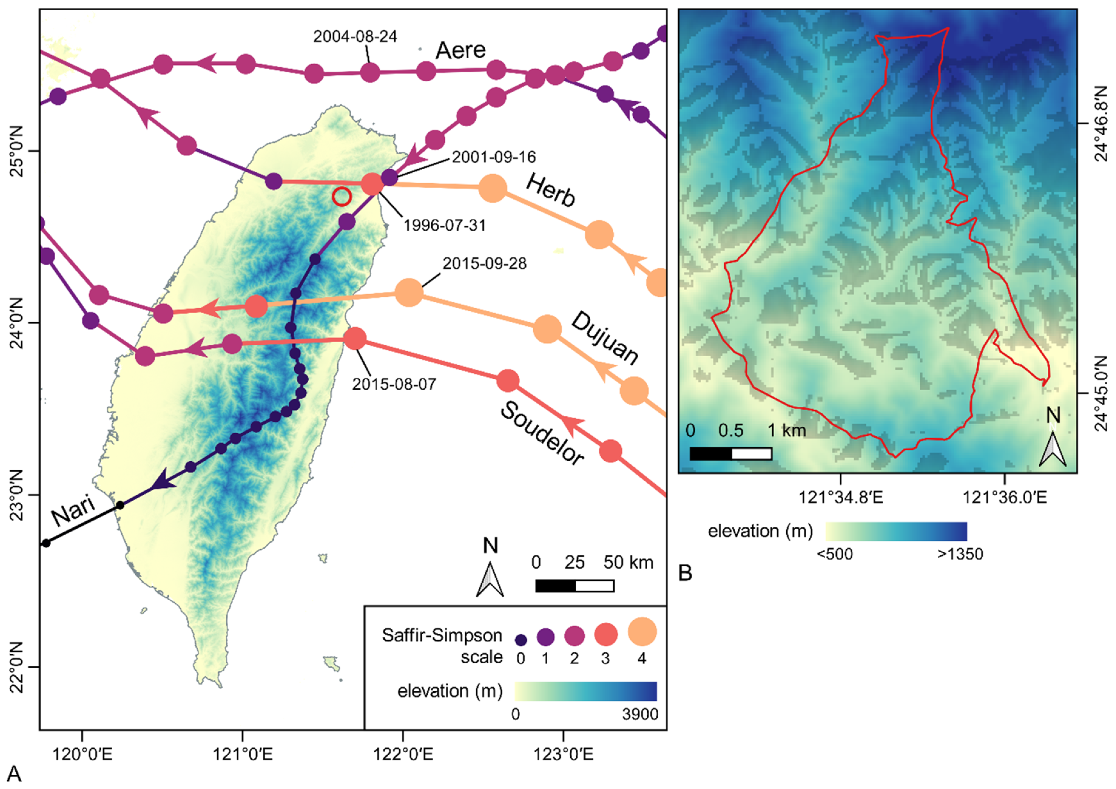
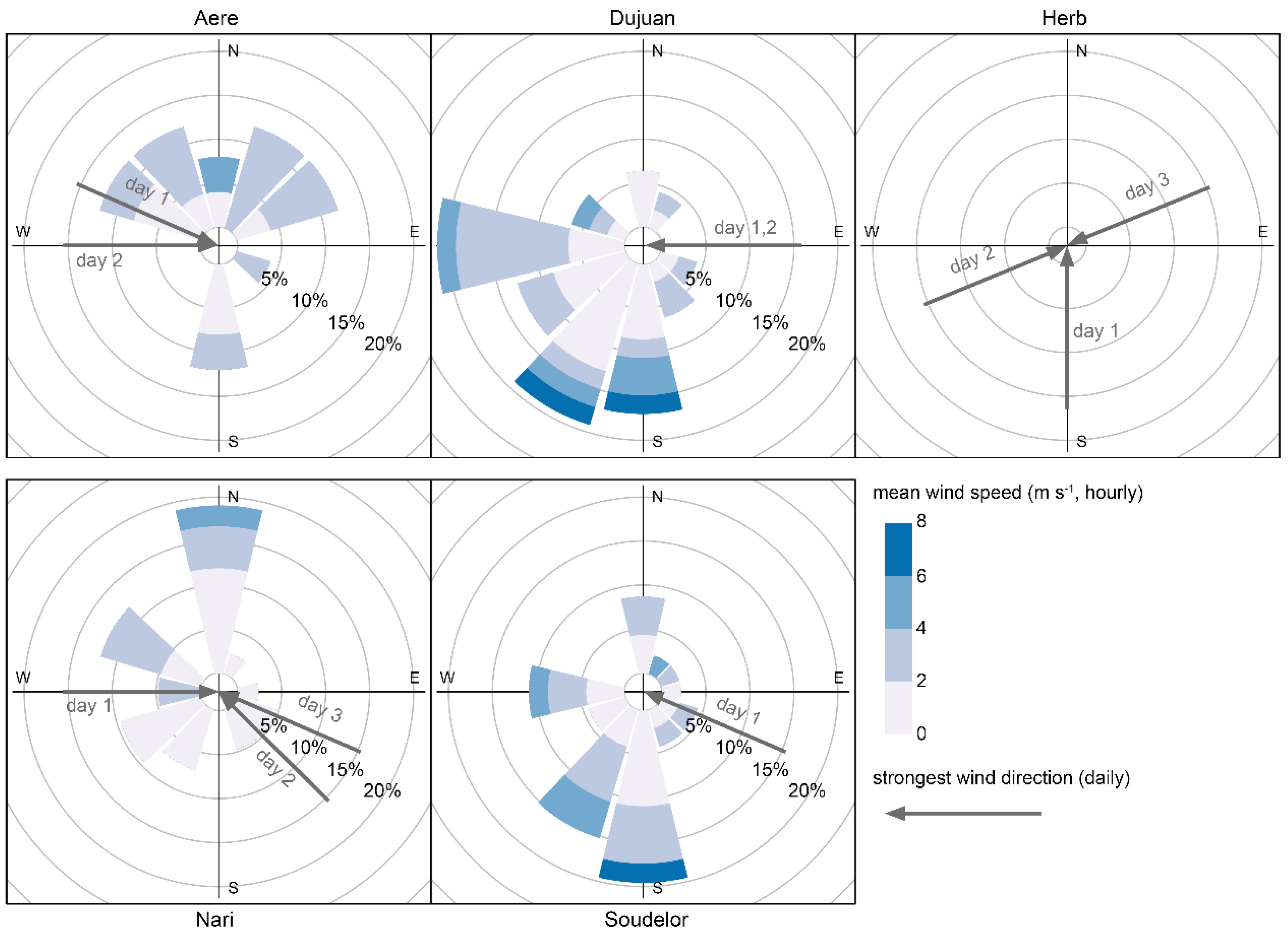
2.1. The Fushan Experimental Forest and Typhoons

The 1000-ha FEF is a nature reserve located in northeastern Taiwan, approximately 25 km from the east coast of the island (Figure 1). Elevation ranges from 400 to 1400 m above sea level (asl). From 1993 to 2004, mean annual temperature measured 18.2 °C, mean annual precipitation measured 4271 mm, and mean relative humidity was 95% [67,68]. The forest is classified as an old-growth sub-montane evergreen broadleaf forest dominated by trees species of Lauraceae and Fagaceae [67,68,69].

The FEF is regularly affected by typhoons between June and October, with an average of 0.74 typhoons per year between 1951 and 2005 [64]. Five recent typhoons (Herb, Nari, Aere, Soudelor, and Dujuan) were selected based on the availability of Landsat images with less than 50% cloud cover of the FEF within seven weeks of the typhoon passage ([23,72] but see [44,73]). We chose the temporal limit of seven weeks in order to minimize any changes in leaf phenology, which can occur within a matter of weeks. Although 50% cloud cover is substantial, it is difficult to find images with low cloud cover in cyclone-impacted regions [44], especially for the FEF, where it rains more than 220 days per year on average [74]. The five typhoons passed within 100 km of the FEF, and were all category 2 or 3 on the Saffir–Simpson scale ([75], Figure 1). Given that each of the typhoon air masses were within 100 km of the FEF, a distance envelope within which winds are strongest, the FEF was affected by all five typhoons.

According to the IBTrACS cyclone tracks dataset [70,71], Typhoon Herb (1996, category 3) was the first typhoon of its season to cross the 100-km range envelope of the FEF. In contrast, Typhoon Nari (September 16th 2001) was preceded by Typhoon Toraji, which passed in proximity to the FEF on July 29th–30th (categories 3 to 1), and Tropical Storm Mindulle (July 4th to 5th 2004) preceded Typhoon Aere (August 8th 2004). No typhoon made landfall before Soudelor and Dujuan (2015) near the FEF, and the two typhoons were seven weeks apart (Figure 1). Among the studied typhoons, Typhoon Aere did not make landfall, but its center was 80 km from the FEF at its closest point. All typhoons were associated with high rainfall (690–1300 mm), and winds over 20 m s⁻¹ at the FEF (

Table 1. Total rainfall (mm) and maximum wind speed measured at the Fushan Experimental Forest during the periods associated with the five typhoon passages. Data from the Fushan meteorological stations (Central Weather Bureau of Taiwan).

Typhoon	Dates	Total Rainfall (mm)	Max Instantaneous Wind Speed (m s−1)
Herb	1996-07-30 to 1996-08-01	720	36.8
Nari	2001-09-16 to 2001-09-18	1300	25.1
Aere	2004-08-24 to 2004-08-25	710	25.0
Soudelor	2015-08-07 to 2015-08-08	790	21.8
Dujuan	2015-09-28 to 2018-09-29	690	21.9

). Nari was the wettest typhoon, whereas Herb had the highest wind speed (Table 1).

The winds of the typhoons had different trajectories (Figure 2). The winds of Soudelor and Dujuan were mostly out of the south and west, whereas the winds of Nari and Aere were of northern origin (Figure 2). Although within each typhoon, at the hourly timescale, wind direction and speed were largely consistent, and daily data showed that the strongest wind gusts could come from different directions.

2.2. Satellite Images

Landsat images were used to analyze vegetation cover change and recovery within the FEF in relation to typhoon disturbances. For each typhoon, pre- and post-disturbance images were taken within seven weeks of the typhoon passage to minimize phenological change in vegetation cover [77,78]. Images used to study vegetation recovery were taken during the growth season before typhoon passage, and one year later during at a comparable time with minimal cloud cover. However, the recovery associated with Typhoon Herb was not studied because of the lack of images with low cloud cover. Basic information on the images used in this study is given in

Table 2. Basic information on Landsat images used in this study. Null cells were either covered by clouds or defined as non-forested using the Global Forest Cover dataset [80]. Pre- and post-disturbance images are shown in Figure S1.

Typhoon	Image Acquisition Dates		Sensors	Resolution (m)	Null Cells (%)
	disturbance	recovery
Herb	1996-07-06 & 08-23	-	TM5	30	19.4
Nari	2001-09-14 & 10-08	2001-06-18 & 2002-06-29	TM5, ETM+	30	17.5
Aere	2004-07-12 & 09-30	2004-07-12 & 2005-07-15	TM5	30	30.8
Soudelor	2015-06-09 & 08-12	2015-06-09 & 2016-07-13	OLI	30	48.8
Dujuan	2015-09-13 & 11-16		OLI	30	33.9

, images used to study pre- and post-typhoon states are shown in Figure S1 in the Supplementary Material. Data from satellites Landsat 5, 7, and 8 were downloaded from the EarthExplorer website [79] as surface reflectance at 30 m resolution, with atmospheric and radiometric corrections performed with the LEDAPS (Typhoons Aere, Herb and Nari) or LaSRC (Typhoons Dujuan and Soudelor) algorithm. A digital elevation model (DEM) at a 30-m spatial resolution was downloaded from the ALOS World 3D dataset from JAXA. Non-forested surfaces were identified with the Global Forest Cover dataset version 1.5 (GFC, [80]).

2.3. Pre-Processing

Pre-processing of spectral data followed [81]. Rasters were topographically corrected using the C correction method with the topcor function of the ‘RStoolbox’ package [82] in R 3.6.1 [83]. Clouds and shadows were identified based on the Pixel QA band provided by the USGS, and derived from [84] with CFmask detection algorithm and visual inspection of true color composite (i.e., for Nari recovery) before being removed from all rasters. In addition, non-forested surfaces were identified and removed using the GFC dataset with a threshold of 75% following studies of other tropical moist forests [85,86].

2.4. Processing

Three topographical variables were derived from the DEM using the terrain function from the ‘raster’ R package [87]: slope steepness, slope aspect, and topographic position index (TPI). The TPI is derived from the type of terrain surrounding a particular cell, with values ranging between −10 and 10. A TPI value of 0 indicates flat terrain surrounds the cell, whereas a cell surrounded by lower terrain has a positive TPI and a cell surrounded by more elevated terrain has a negative TPI. Aspect numerical values were converted into eight categorical variables (e.g., north, northeast, etc.) covering 45° each, centered on the cardinal direction (e.g., from 22.5° to 67.5° for northeast). TPI values were converted into six slope positions following [88] as described in

Table 3. Conversion thresholds of topographic position index (TPI) to slope positions and based on standard deviation (SD) of TPI and slope steepness following [88].

Slope Position	TPI	Slope (°)
Ridge	SD < x	–
Upper slope	0.5 SD < x < SD	–
Middle slope	−0.5 SD < x < 0.5 SD	>5
Flat slope	−0.5 SD < x < 0.5 SD	<5
Lower slope	−SD < x < −0.5 SD	–
Valley	x < −SD	–

. Slope steepness was used to differentiate middle slope from flat slope areas, because the two had the same TPI value range (Table 3).

Four commonly used VIs were created using the surface reflectance rasters NDVI (Equation (1), [89]), NDII (Equation (2), [60]), EVI (Equation (3), [55]), and SAVI (Equation (4) [90]). Although NDVI has been widely used in ecological studies (see reviews by [48,50,51]), it saturates faster than EVI and NDII at high biomass densities [55]. In contrast, EVI is more sensitive than NDVI to vegetation changes in areas with high biomass [91]. NDII has been shown to provide better monitoring of canopy defoliation and damage to forest structure [92,93,94], while SAVI reduces the soil effect [90]. The four indices are the products of four bands from the Landsat sensors: blue (B), red (R), NIR, and the first short-wave infrared band (SWIR1).

$$\mathrm{NDVI}=\frac{NIR-R}{NIR+R}$$

(1)

$$\mathrm{NDII}=\frac{NIR-SWIR1}{NIR+SWIR1}$$

(2)

$$\mathrm{EVI}=G\times \frac{\left(NIR-R\right)}{\left(NIR+C1\times R-C2\times B+L\right)}$$

(3)

$$\mathrm{SAVI}=\frac{\left(1+L\right)\left(NIR-R\right)}{\left(NIR+R+L_2\right)}$$

(4)

In the equation of EVI, the coefficients for EVI are the gain factor, G = 2.5; the canopy background adjustment, L = 1; and two coefficients of aerosol resistance, C1 = 6 and C2 = 7.5 [95]. For SAVI, the canopy density adjustment L2 = 0.5 [90].

To measure the effects of typhoon disturbance, the variation in VI was calculated using Equation (5). A negative ΔVI indicates a decrease in vegetation cover post-disturbance.

$$\Delta \mathrm{VI}=V{I}_{post-disturbance}-V{I}_{pre-disturbance}$$

(5)

2.5. Analysis of Disturbances among Vegetation Indices

Typhoon effects on VIs were first analyzed separately for each of the five typhoons, in which only cloudy cells in the images related to the given event were excluded from the analysis. In contrast, only the shared non-clouded cells were used for cross-typhoon comparisons. For each typhoon, the ΔVI was compared to 0 with a one-sample Wilcoxon signed-rank test. Then, Spearman’s ρ was used to explore the relationships among the four ΔVIs (very weak < 0.2 < weak < 0.4 < moderate < 0.6 < strong < 0.8 < very strong) with the corr.test function from the ‘psych’ R package and p adjustment of Bonferroni for multiple comparisons [96]. In addition, the same test was used to study the correlations between pre-disturbance state ($V{I}_{pre-disturbance}$) and the ΔVIs to examine if the changes in VIs are related to pre-disturbance vegetation conditions.

Across all typhoons, correlations between individual ΔVI (e.g., ΔNDVI among the five typhoons) were tested with Spearman’s ρ to examine the consistency of vegetation damage detection among different VIs. Furthermore, to assess the effects of each typhoon disturbance on vegetation, coefficients of variation (CV) of each VI before and after disturbances were compared through a bootstrapped comparison of means (5000 iterations) using Equation (6).

$$C{V}_{post-disturbance}-C{V}_{pre-disturbance}$$

(6)

2.6. Typhoon Damages and Topography

The relationships between ΔVIs and topographical variables were analyzed with ordinary least-squares (OLS) regression models, which are commonly used in forest ecology [97,98,99], including elevation and slope as continuous parameters, and TPI and aspect classes as ordinal variables. The number of cloud free pixels across all the images used for model construction was 4593.

2.7. Disturbance Frequencies and Intensity

Damage frequency was defined as the number of typhoons (out of 5) affecting a particular cell. Small variations in VI unrelated to wind damage may cause negative values; therefore, a more conservative threshold than < 0 was used to identify typhoon-damaged cells (Equation (7)). Only ΔNDII and ΔEVI were used in this analysis, whereas ΔNDVI and ΔSAVI were not included because of their moderate-to-strong correlations with ΔNDII and ΔEVI (ρ values ranging from 0.48 to 0.97). To assess if more frequently disturbed cells (i.e., those with frequencies of 4 or 5) were also more severely disturbed (had more negative ΔVI), mean ΔVIs among the six frequency classes were compared using the multiple comparisons procedure described by [100] for unbalanced designs with unequal variances with the ‘multcomp’ [101] and ‘sandwich’ [102,103] packages. Similarly, TPI-derived classes as well as aspect classes were compared to examine if cells containing certain topographical features were more frequently affected by typhoons. Relationships between elevation and slope with damage frequencies were tested using OLS regressions.

$$\Delta \mathrm{VI}<{\mathrm{mean}}_{VI}-0.5\times {\mathrm{SD}}_{VI}$$

(7)

2.8. Vegetation Recovery

Forest canopy recovery following Typhoons Aere, Nari, and Soudelor–Dujuan was analyzed by comparing an image of the FEF before disturbance to an image taken a year later during the same season (i.e., after disturbance, Table 2) through bootstrapped comparisons on means (5000 iterations). Typhoons Soudelor and Dujuan, which were only seven weeks apart, were studied together, as it was not possible to separate their recovery. Typhoon Herb could not be included in the recovery analysis due to the lack of images with low cloud cover following the typhoon.

3. Results

3.1. Vegetation Indices, Typhoons, and the Effect of Prior Vegetation Cover

The four VIs all significantly decreased after the five typhoons (one sample Wilcoxon, V = 63,407 to 42,679,021, all p-values < 0.001, sample size = 6361 to 10,128) except for the significant increase of NDII, EVI, and SAVI associated with Typhoon Herb (all p-values < 0.001,

Table 4. Average change (standard deviation) in vegetation indices (VIs) over five typhoon intervals for the Fushan Experimental Forest. ΔVIs are calculated as the difference between post- and pre-typhoon values for five typhoons, so negative values indicate vegetation loss (Equation (5)). Averages are calculated on variable portions of the Fushan Experimental Forest as the cloud cover varies among the images used to study typhoon events (see Table 2).

	Vegetation change
Typhoon	ΔEVI	ΔNDII	ΔNDVI	ΔSAVI
Aere	−0.021 (0.047)	−0.006 (0.034)	−0.012 (0.027)	−0.029 (0.038)
variation (%)	−3.39	−1.18	−1.39	−5.34
Dujuan	−0.121 (0.057)	−0.044 (0.031)	−0.012 (0.034)	−0.089 (0.041)
variation (%)	−19.87	−12.09	−1.19	−16.23
Herb	0.048 (0.099)	0.008 (0.045)	−0.035 (0.067)	0.014 (0.423)
variation (%)	11.06	3.31	−4.01	4.01
Nari	−0.046 (0.050)	−0.034 (0.037)	−0.044 (0.071)	−0.052 (0.040)
variation (%)	−8.62	−9.87	−5.51	−12.50
Soudelor	−0.010 (0.045)	−0.017 (0.027)	−0.022 (0.033)	−0.010 (0.037)
variation (%)	−1.34	−4.40	−2.52	−1.55

). Compared to the pre-typhoon VI values, the decrease was greatest for Dujuan and smallest for Aere and Soudelor (Table 4).

Correlations among ΔVIs were significant for all typhoons, although they varied in strength (

Table 5. Spearman’s correlations among the four ΔVIs measured over five typhoons for the Fushan Experimental Forest. All correlations are statistically significant (p-values < 0.01). ΔVIs are calculated as the difference between post- and pre-typhoon values (Equation (5)). The relationships are studied on variable portions of the Fushan Experimental Forest as the cloud cover varied among the images (see Table 2).

	Correlation (ρ)
Typhoon	ΔEVI-ΔNDVI	ΔEVI-ΔNDII	ΔEVI-ΔSAVI	ΔNDVI-ΔNDII	ΔNDVI-ΔSAVI	ΔNDII-ΔSAVI
Aere	0.59	0.23	0.90	0.28	0.64	0.31
Dujuan	0.27	0.21	0.90	0.48	0.19	0.19
Herb	−0.23	−0.27	0.60	0.64	0.42	0.26
Nari	0.10	0.05	0.48	0.56	0.80	0.55
Soudelor	0.39	0.46	0.97	0.64	0.48	0.49

). All the correlations were positive except for those between ΔEVI–ΔNDVI and ΔEVI–ΔNDII. Most of the correlations were weak to moderate (ρ = 0.05–0.50) but the correlations between ΔEVI and ΔSAVI were generally strong (ρ up to 0.90) (Table 5). Pre-disturbance VIs and ΔVIs had significant negative correlations in all cases (p < 0.001, Table S1). These relationships were in general weak for Typhoons Dujuan and Nari and considerably stronger for Typhoons Aere, Herb and Soudelor (Table S1).

3.2. Variation of ΔVIs among Typhoons

The correlations of ΔVIs among typhoons were mostly negative between Typhoon Dujuan and other typhoons and mostly positive among other typhoons (Table S2). Most of the correlations were either weak, very weak or not significant. However, moderate positive correlations were detected for the ΔNDVI of Typhoon Herb–Soudelor, Herb–Nari and Soudelor–Nari (Table S2).

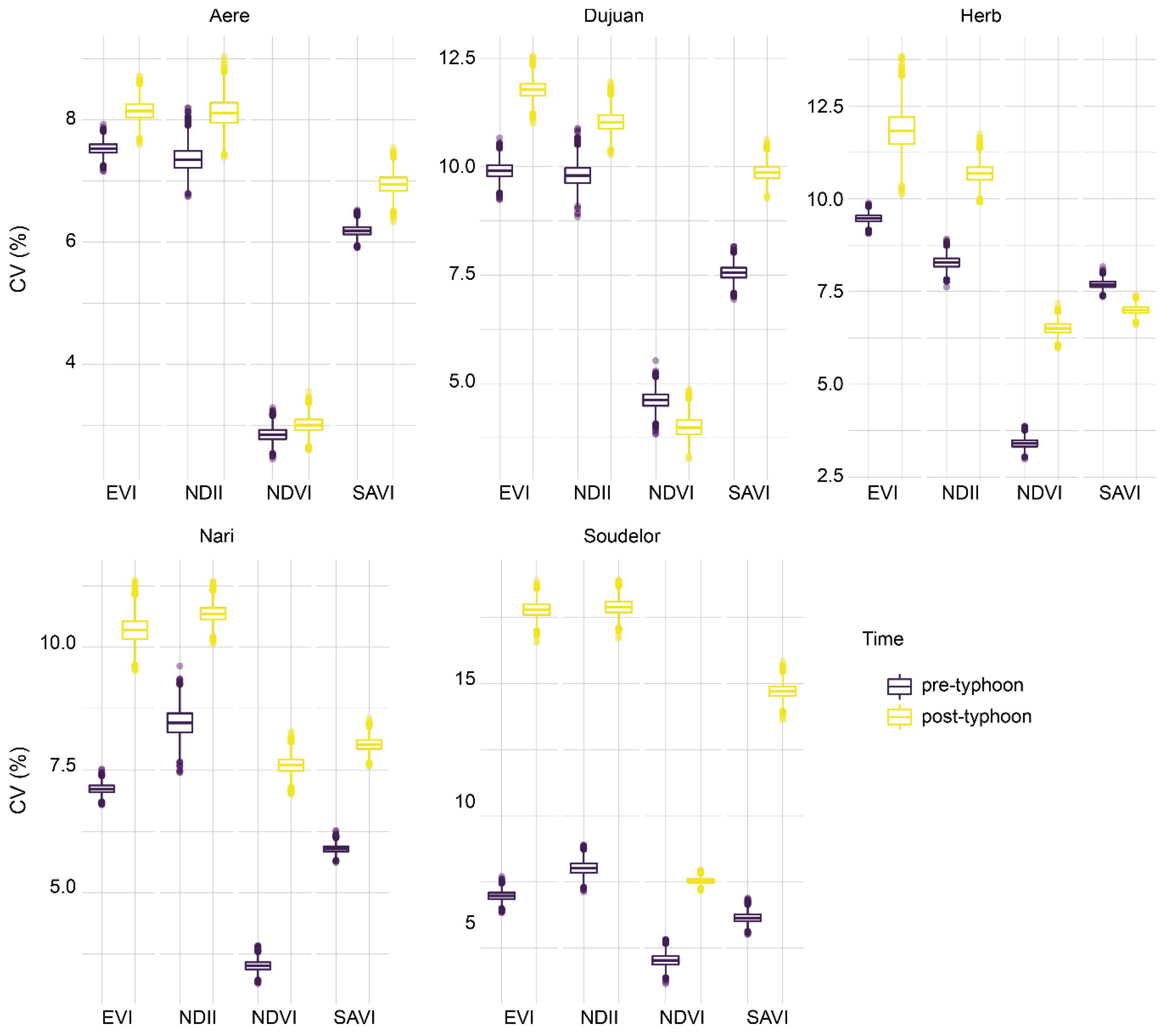
3.3. Effects on Vegetation Heterogeneity

Except for SAVI in relation to Typhoon Herb, typhoons led to a higher heterogeneity in VI values, as indicated by the significantly greater post-typhoon CV of all VIs except for NDVI for Typhoons Aere and Dujuan, wherein the CV did not change significantly (Figure 3).

3.4. Topography and Disturbance Severity

Topographical variables differed in their ability to explain the variation of ΔVIs among the typhoons (

Table 6. β Coefficients of ordinary least squares linear models between topographical variables and changes in vegetation index values (ΔVIs) associated with Typhoons Nari and Herb. Sample size of 4593 (equal to the number of pixels from analyzed Landsat images). Significance levels are shown with ^† (p < 0.05), ^‡ (p < 0.01), and * (p < 0.001). Only the first non-zero value is shown, complete results for the five typhoons are in Table S3.

Topography	Nari				Herb
	ΔEVI	ΔNDII	ΔNDVI	ΔSAVI	ΔEVI	ΔNDII	ΔNDVI	ΔSAVI
Elevation (m)	0.00005 *	0.00002 ‡	0.00008 *	0.00006 *	0.0002 *	0.0001 *	0.0002 *	0.0002 *
Slope (°)	0.0006 *	−0.001 *	−0.002 *	−0.0008 *	0.002 *	−0.0007 *	−0.001 *	0.0002 *
TPI category
Lower slope	−0.008	0.003	0.007	0.003	0.02 †	0.02 *	0.02 *	0.02 *
Middle slope	−0.005	0.003	0.008	0.005	0.03 *	0.03 *	0.02 *	0.02 *
Ridge	−0.0005	0.0004	0.004	0.008 ‡	0.03 *	0.03 *	0.02 *	0.02 *
Upper slope	−0.002	0.002	0.005	0.006 †	0.03 *	0.03 *	0.02 *	0.02 *
Valley	−0.008	0.0007	0.003	0.0001	0.01	0.02 *	0.01 *	0.01 *
Flat slope	-	-	-	-	-	-	-	-
Aspects
North	0.007 ‡	−0.03 *	−0.07 *	−0.03 *	0.03 *	−0.03 *	−0.05 *	−0.005 ‡
Northeast	−0.002	−0.02 *	−0.03 *	−0.01 *	0.005	−0.006 ‡	−0.01 *	−0.003
Northwest	0.02 *	−0.03 *	−0.09 *	−0.04 *	0.05 *	−0.06 *	−0.09 *	−0.02 *
South	−0.006 ‡	−0.0005	−0.001	−0.006 *	0.02 *	−0.03 *	−0.04 *	0.0004
Southeast	−0.003	−0.0002	0.006 †	−0.003	0.006	−0.007 *	−0.01 *	−0.001
Southwest	−0.006 †	−0.01 *	−0.03 *	−0.02 *	0.05 *	−0.05 *	−0.07 *	−0.0005
West	0.009 *	−0.02 *	−0.06 *	−0.03 *	0.07 *	−0.06 *	−0.1 *	−0.007 *
East	-	-	-	-	-	-	-	-
R2	0.07899	0.2163	0.4684	0.2786	0.2222	0.3417	0.5179	0.2046
Adjusted R2	0.07618	0.2139	0.4668	0.2764	0.2198	0.3397	0.5164	0.2021

for Nari and Herb, Table S3 for other typhoons). Topography was a better predictor of ΔNDVI for typhoons Herb and Nari (adjusted R² = 0.52 and 0.47, respectively) than it was for other ΔVIs (adjusted R² ≤ 0.34). For typhoons Aere, Dujuan, and Soudelor that passed further from the FEF (Figure 1), topographical variables were poor predictors of ΔVI values (adjusted R² ≤ 0.16). Elevation and slope were significant in explaining ΔVI variation in all cases except slope for ΔEVI and ΔSAVI for typhoon Dujuan (p > 0.05, Table 6 and Table S3); however, coefficients were small (β < 0.0002 for elevation, β < 0.008 for slope). The magnitude of ΔVI decreased with increasing topographic slope for all VI–typhoon combinations, except for ΔEVI with typhoons Herb and Nari, and ΔSAVI with typhoon Herb. However, increasing elevation led to either higher or lower damage (i.e., change in VI) depending on the typhoon in question, but the change in direction was consistent among VIs for each typhoon. Except for flat slopes, all TPI positions had positive and statistically significant (p < 0.05) regression slope coefficients for Soudelor, Nari, Herb and Aere. On the other hand, Typhoon Dujuan showed negative relationships for all TPI positions except for flat slopes. Nevertheless, the sign of regression slope coefficients remained consistent among ΔVIs for each typhoon. The relationships between aspect and ΔVI values changed among typhoons, showing no clear pattern.

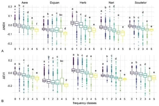
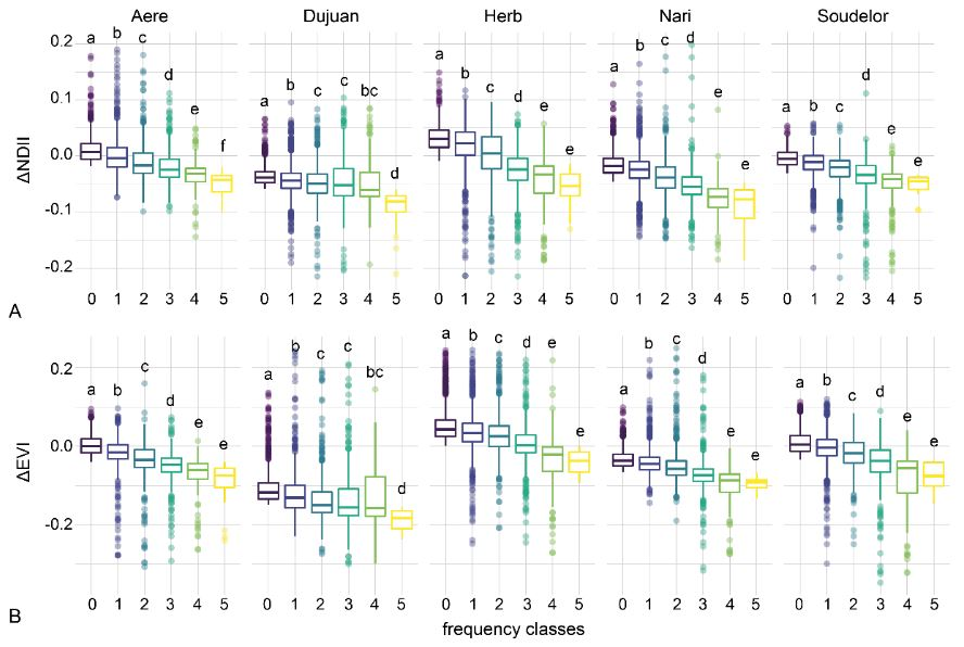
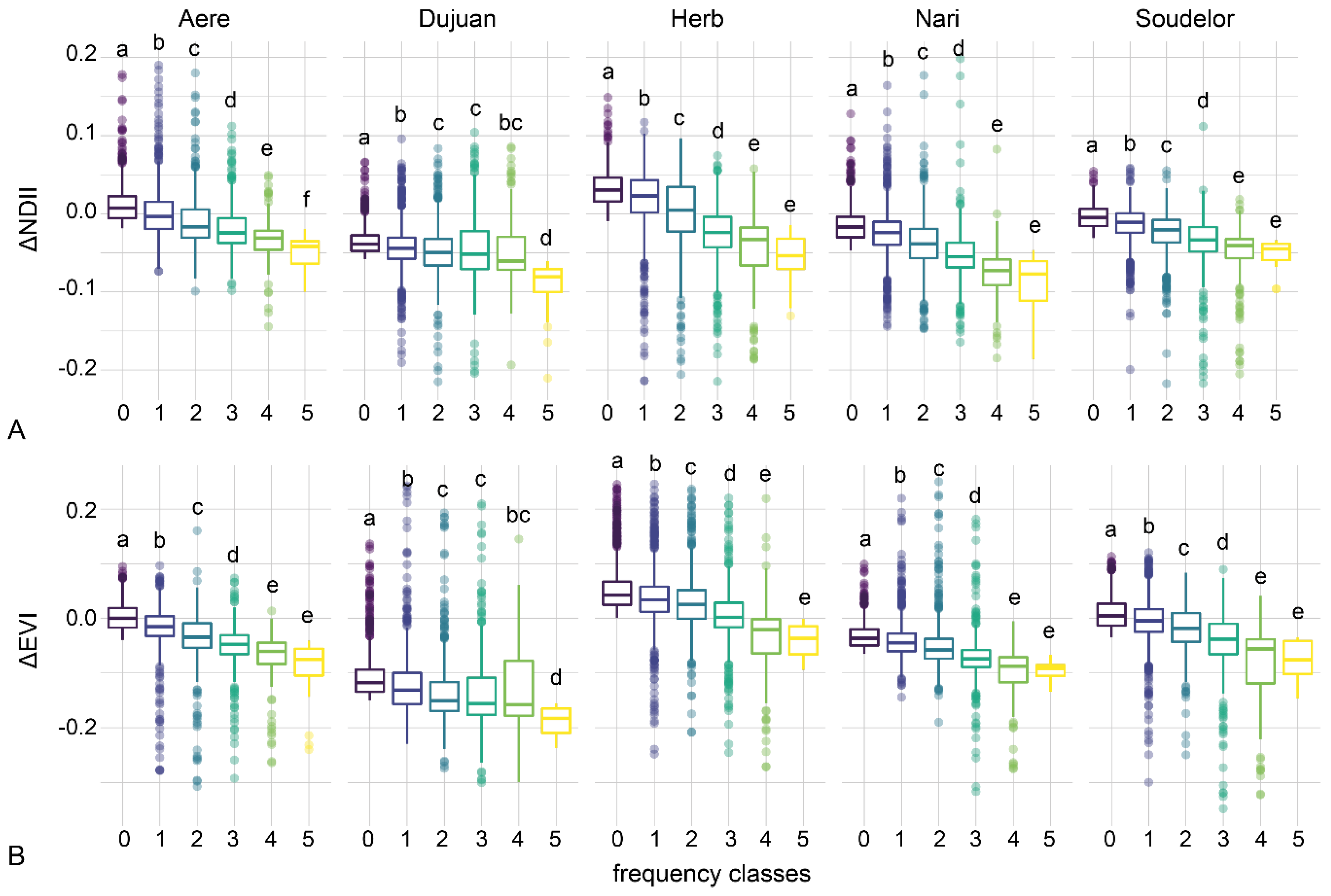
3.5. Disturbance Frequency and Severity

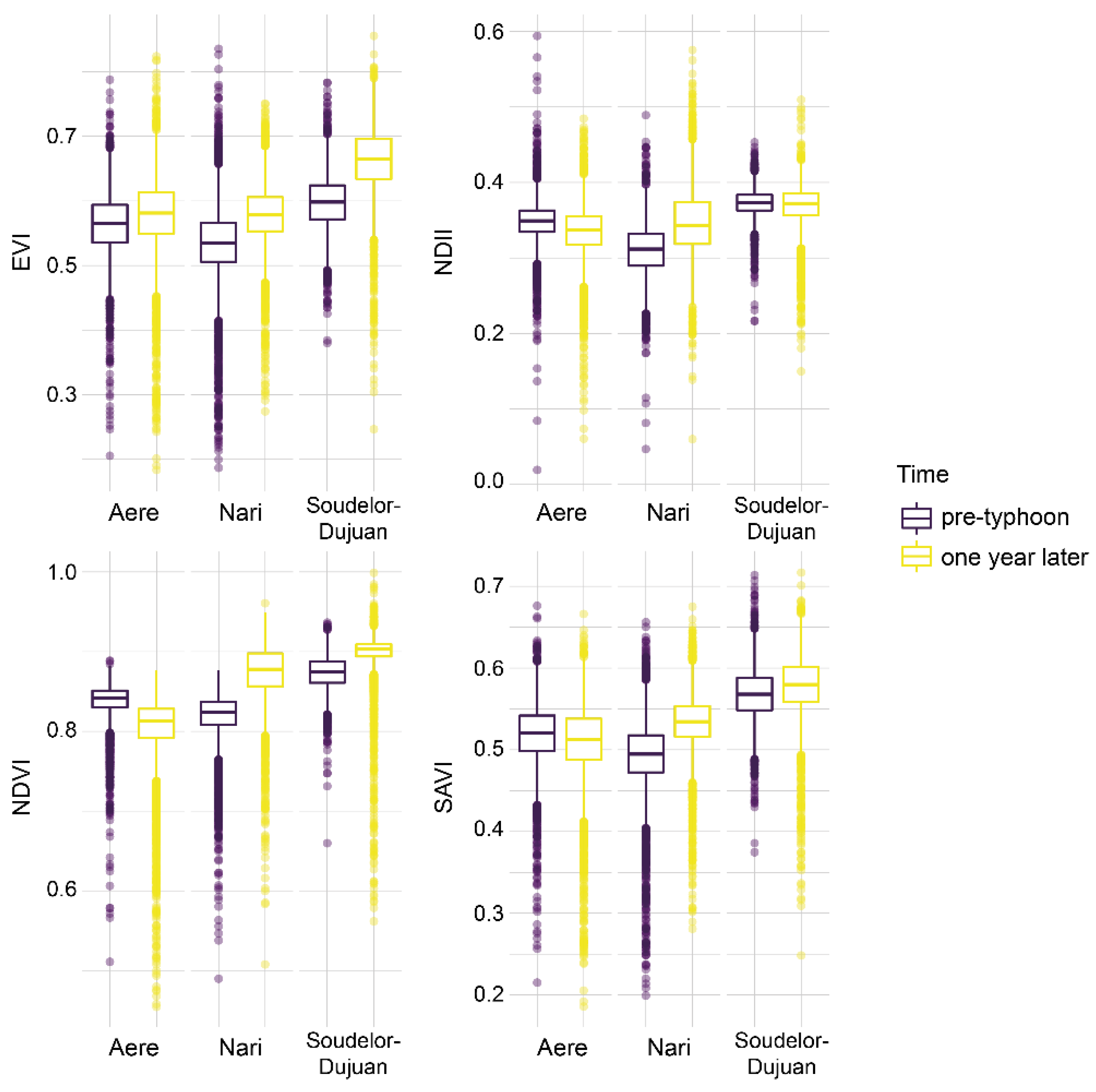
For all typhoons but Dujuan, the more frequently affected cells had greater VI losses (Figure 4). Typhoon damage frequency varied with elevation and slope steepness. Elevation was negatively related to EVI-based damage frequencies (β = −6.71, p < 0.001, adjusted R² = 0.016) but not to NDII-based frequencies (p = 0.47). On the other hand, slope was positively related to EVI- and NDII-based frequencies (β = 0.32, adjusted R² = 0.001, p = 0.01 for EVI; β = 2.16, adjusted R² = 0.07, p < 0.001 for NDII). The proportion of damage frequency varied among aspects (Figure 5, Table S4). For NDII, all aspects were significantly different in damage frequency (p < 0.001), except for south–east, northeast–north, southwest–northeast, southwest–north, and west–northwest (p > 0.05, Table S4). For NDII, southwestern to northwestern aspects had the highest damage frequencies and southeastern aspects had the lowest disturbance frequency (Figure 5A). Considering EVI, northern aspects had more frequent typhoon damage than western and southern aspects, whereas there were no significant differences between other aspects (Table S4, Figure 5B). Among slope positions, according to EVI, the flat slope, lower slope, and valley positions had similar typhoon damage frequencies (Table S4); these three topographic positions were more frequently damaged than other positions. For EVI, ridge areas had lower typhoon damage frequency than all other slope positions (Table S4). With NDII-based frequencies, no significant differences were observed between rides and slope or among other topographical positions (p > 0.05 with adjustment, Table S4).

3.6. Recovery

Vegetation cover had recovered in less than a year after Nari, as average VI values measured in June 2002 were equal to or greater than their values in June 2001 (positive 95% CIs, Figure 6). Similarly, all Vis, except NDII, registered vegetation recovery in less than one year after typhoons Soudelor–Dujuan (Figure 6). In contrast, EVI was the only VI showing recovery after Aere (Figure 6).

4. Discussion

4.1. Consistency in the Damage Effects among Typhoons

The consistent decrease in VI values following all five typhoons (with very few exceptions; see Table 4) suggest that all the VIs can generally capture typhoon-induced losses in vegetation cover [23,24,43,104,105,106]. However, we find weak correlations in ΔVIs between different typhoon events (ρ < 0.4, Table S2), indicating that typhoons range in their effects on vegetation cover. Although this is not surprising because typhoons differ in intensity, duration, trajectory and occurrence time relative to plant phenology, the inconsistency among vegetation indices highlights that results derived from one or a few disturbance events are unlikely to represent general trends in disturbance effects. Indeed, our results show that the successive Typhoons Soudelor and Dujuan did not have consistent effects on vegetation although they had comparable paths, wind speeds, and directions (Figure 1 and Figure 2, Table 1). Additionally, the very weak negative correlations of the ΔVIs between typhoons Soudelor and Dujuan (Table S2) indicate that the two typhoons had different effects on the vegetation cover, as observed in other sites subject to successive cyclones [21,22,107].

Powerful cyclones, such as Hurricanes Hugo and Maria in Puerto Rico, Typhoon Herb in Taiwan, and Cyclone Larry in northeastern Australia, attract scientific study of their ecological effects [25,26,35,38,40,43,106,107,108,109,110,111]. This high prevalence of studies has advanced our understanding of cyclone ecology, especially in relation to the most powerful and damaging storms (reviewed by [12,14,112]). However, in this study, Typhoon Herb was considered to be the most powerful typhoon in several decades [113]. Typhoon Herb had the greatest wind speed among the five typhoons studied, while Nari was most intense in terms of precipitation. Considering these two storms, the resultant changes in vegetation index values (ΔVIs) were only weakly correlated. Future increases in the frequency of the most intense cyclones are predicted [114,115,116]. However, our results suggest that conclusions drawn from studies that document the effects of a single or a few intense cyclones are insufficient for predicting the effects of future cyclones.

The fact that there were small or no changes in VIs associated with Typhoon Herb is somewhat surprising. In addition to the potential influence of image quality on our analyses, the timing of Typhoon Herb is probably the most important factor. Typhoon Herb occurred in the summer (late July) when the forest was in the middle of the main growing season, and the two images were approximately two months apart. Thus, plant growth could be substantial during the period, potentially confounding the detection of typhoon-caused decreases in vegetation cover by VIs. This contrasts with Typhoon Dujuan, which caused the largest decreases in VIs. Typhoon Dujuan occurred near the end of the main growing season (April to September) so that although the two images were also approximately two months apart, there was little vegetation growth during the period. As a result, typhoon-induced vegetation loss can be better detected with the VIs. Thus, image timing in relation to plant growth phenology should be considered when examining disturbance-induced changes in vegetation cover using VIs.

Not only were the overall effects inconsistent among typhoons, there was large variation in linear regression results, which showed that typhoon damage–topography relationships were inconsistent among typhoons (Table 6 and Table S3). Topography was better at explaining disturbance distribution across the landscape for Typhoons Herb and Nari, the typhoons that passed the closest to the FEF, but they were not the storms that caused the greatest degree of vegetation damage. This result suggests that topography–vegetation damage relationships vary with cyclone distance and that topography is a key determinant of vegetation damage only when typhoons are very close to the study site, despite the magnitude of the damage. It also suggests that factors other than cyclone distance determine the severity of typhoon-induced vegetation cover damage.

Nevertheless, there were some consistencies across typhoons. First, the canopy generally recovered quickly as many VIs returned to their pre-disturbance values within a year (Figure 6). This result is consistent with the report of the rapid recovery of the FEF observed following Typhoon Bilis using NDVI [106]. However, recovery of a VI does not imply total canopy recovery as LAI and litterfall typically do not recover within a year of damage in the FEF [73]. Second, the relationship between high pre-disturbance NDVI and strong NDVI loss observed by [106] was also detected for all five typhoons in this study despite their differences in paths and intensities (Table S1). This pattern may be explained by the higher aerodynamic drag of dense canopies as suggested by [16], who reported a similar relationship between pre-disturbance LAI and LAI loss (see also [17]). Third, cyclones are disturbance agents which induce heterogeneity in forest landscapes [14,64]. Secondary tree falls and defoliation may have led to the increased heterogeneity observed following almost all typhoons examined here. Finally, most ΔVIs were positively correlated between typhoons (Table S2), except for Soudelor–Dujuan, suggesting that different typhoons could have similar effects although the strength of the relationships varied greatly among typhoons and VIs.

4.2. ΔVIs in Relation to Topography

The topography only explained a small proportion of the variation in vegetation cover change. As observed by [32], steeper slopes were associated with greater decreases of all VIs across all typhoons (Table 6 and Table S3), perhaps because of different wind exposures and soil stability (e.g., landslides, [117]). However, our results show that the relationships between vegetation damage and other topographical variables changed among typhoons and VIs, even when typhoons had similar tracks and wind directions. Thus, observations from a single event should be generalized with caution, as they do not necessarily remain true for other cyclones. Indeed, complex interactions between wind and topography have occurred in the FEF, as leeward positions were more affected than eastern positions for Typhoon Nari but not for Dujuan (Figure 2, Table 6 and Table S3). Less exposed slopes may also offer little protection if the cyclone is particularly strong [40]. The overall low adjusted-R² values indicate that factors other than topography (e.g., vegetation conditions and timing of typhoon disturbance) likely play a more important role in determining typhoon-induced changes in vegetation cover.

4.3. Typhoon Disturbance Frequency

The greater damage for more frequently than less frequently affected cells (Figure 4) is consistent with a study from a moist forest of Puerto Rico, in which trees sustaining heavy damages from Hurricane Hugo (1989) were more likely to be damaged again nine years later by Hurricane George [118]. The result is also consistent with the mostly positive correlations between ΔVI values among the different typhoons (Table S2). Although it is possible that sites with certain topographical features within the FEF are more prone to typhoon damage, this claim is not supported by the lack of consistent topographical damage patterns among typhoons (Table 6 and Table S3). Possibly, susceptibility to damage is more related to weakened vegetation in these sites (i.e., repeated disturbances). Further field-based research may help to separate the effect of forest characteristics, topography, and typhoon frequency on canopy damage at the FEF.

The greater elevational signal in typhoon damage frequencies at lower than at higher elevations based on EVI fits the pattern of greater damage frequency at lower topographic positions (lower-slope, valley) than other positions (e.g., middle- and upper-slope). It also supports results from field observations of greater typhoon effects at low than at high elevations along a 2300-m elevational gradient in central Taiwan [65]. It appears that the elevational pattern is consistent across spatial scales including variation in slope across the landscape, possibly because the intensity of typhoons declines quickly in rough topography as they move upward [65]. The differences in NDII and EVI sensitivity to vegetation characteristics may explain the different relationships of their damage frequencies with slope. As observed in Puerto Rico [36], different aspects had different disturbance frequencies, with northern aspects having significantly higher values. However, the relationship with the windward–leeward direction was less clear here, as western aspects (leeward in the FEF) also had high damage frequencies. The very rough topography at the FEF, with a mean slope of 38%, probably obscures relationships between slope, aspect and typhoon damage.

4.4. Consistency among Vegetation Indices

We did not detect any VI that was consistently the most sensitive across the five typhoons. EVI and NDII were considered particularly functional to measuring vegetation characteristics such as canopy structure [55] and water content [61,62]. However, in our study, they did not detect strong decreases in vegetation cover relative to pre-typhoon values for Typhoon Herb. Such differences may be the product of different damage variations across disturbance events, as reported for other sites [21,22,107]. It may also be due to the phenological change in leaf properties between pre- and post-disturbance images [77,78], although effort was made to minimize such variation by selecting images from within seven weeks of typhoon events.

Surprisingly, NDVI was the only VI that showed a decreasing canopy cover following Typhoon Herb, whereas it was the least practical index for Dujuan and Nari, despite its lack of sensitivity under high LAI [57,58,59]. NDVI was also the only VI that did not detect change in vegetation cover heterogeneity following Typhoons Aere and Dujuan (Figure 3). Overall, NDVI is less sensitive to vegetation cover change in the FEF than the other Vis, as reported for other sites [92,93,94,119], and its sensitivity varied with typhoon events or images. Large variability between VIs in their responses to disturbance also took the form of varying correlation strength and direction between and within typhoon events (Table 5). However, ΔVIs based on the same spectral bands, such as ΔEVI–ΔSAVI, had stronger correlations than in other cases (e.g., ΔEVI–ΔNDII). The disparity between ΔVIs for a given typhoon suggests that cross-study comparisons of disturbance effects based on several or different VIs could be problematic.

ΔVIs shared some consistencies, nonetheless, as most VIs indicated increasing heterogeneity, and varied somehow similarly with elevation, slope, and TPI-derived classes for each typhoon (Table 6, Table S3). In addition, both ΔNDII and ΔEVI detected increasing severity for more frequent canopy damage.

Our study has several constrains. First, although we compared the consistency among different VIs, we could not identify which VI was more accurate in detecting vegetation changes caused by typhoons due to the lack of ground truthing. Conducting ground truthing is difficult, because although the beginning and the end of typhoon seasons are relatively well understood, typhoon events themselves are unpredictable, hence it is difficult to coordinate ground surveys across the studied landscape without knowing whether a disturbance will occur and where clouds would be present on the satellite images. Although it was possible to conduct ground truthing for past disturbance events, we strongly recommend routine ground surveys on several widely spread plots for studies that aim to assess disturbance effects on vegetation whenever possible. Such ground truthing could help to identify which VI would provide most accurate detection of disturbance-induced vegetation changes.

Second, some of our results may have been affected by cloud obstruction in analyzed images, which is substantial for all images used in this study (17.5–48.8%). A previous study showed that cloud contamination does not distribute across the FEF, with more cloud cover at higher elevations [66]. Because typhoon-induced vegetation change varied with elevation (Table 6), the observed topographical patterns of vegetation change are likely affected to some degree by the non-random cloud contamination. Unfortunately, cloud contamination is common in the FEF and most humid forests. In fact, cloud cover prevented the inclusion of Typhoon Herb in our analyses of vegetation recovery. Third, ideally, images should be derived from the same sensor as different sensors vary in the width of their spectral bands [120] and radiometric calibrations [121,122]. However, we were constrained by the availability of high-quality (low cloud contamination) images because we studied five typhoons spanning over two decades. With the rapid advancement of remote sensing, high-quality images from the same sensor should be increasingly available.

5. Conclusions

Comparison of the effects of five major typhoons affecting the Fushan Experimental Forest (FEF) showed substantial differences as well as some consistency in their effects. First, while typhoons all led to decreases in vegetation index (VI) values, the magnitude of change (ΔVIs) differed among events. The variability of ΔVIs among typhoons may be the product of complex interactions of their characteristics with landscape topography and the biotic conditions when the forest was disturbed (e.g., recovering from previous disturbance, soil moisture). Indeed, topography alone did not explain variation in ΔVIs among typhoons, and its explanatory power varied among the different indices. However, all typhoons shared the same positive relationship between damage severity and pre-disturbance vegetation condition, and all typhoons resulted in increased vegetation heterogeneity. Hence, conclusions drawn from the remote sensing studies of one typhoon may or may not stand for other typhoons in the same landscape, depending on the aspects of the effects under concern. Second, observation of greater disturbance severity for more frequently damaged cells of the FEF shows that some sites are more prone (i.e., have decreased resistance) to disturbances than others. On the other hand, the landscape generally has high resilience in order to maintain its forest cover over the many centuries of typhoon disturbance. Third, the four vegetation indices had different relationships with canopy cover damage, probably because of their different sensitivities across the light reflectance spectrum. The Normalized Difference Vegetation Index (NDVI) was, overall, less sensitive to change, which supports the findings of previous studies pointing to its saturation and overall limited sensitivity under high-biomass forest conditions. The Soil-Adjusted Vegetation Index (SAVI) and the Enhanced Vegetation Index (EVI) were highly correlated, but EVI was less related to the other two indices. Although the Normalized Difference Infrared Index (NDII) and EVI had the same change in direction after the five typhoons, they differed in the magnitude of change. Hence, we suggest using them together as complementarity Vis, because NDII and EVI are, respectively, based on short-wave infrared and near-infrared, making them sensitive to different characteristics of vegetation.

References

1. Gentry, A.H. Tropical forest biodiversity: Distributional patterns and their conservational significance. Oikos 1992, 63, 19–28. [Google Scholar] [CrossRef]
2. Malhi, Y.; Grace, J. Tropical forests and atmospheric carbon dioxide. Trends Ecol. Evol. 2000, 15, 332–337. [Google Scholar] [CrossRef]
3. Pan, Y.; Birdsey, R.A.; Fang, J.; Houghton, R.; Kauppi, P.E.; Kurz, W.A.; Phillips, O.L.; Shvidenko, A.; Lewis, S.L.; Canadell, J.G.; et al. A large and persistent carbon sink in the world’s forests. Science 2011, 333, 988–993. [Google Scholar] [CrossRef] [PubMed] [Green Version]
4. Beer, C.; Reichstein, M.; Tomelleri, E.; Ciais, P.; Jung, M.; Carvalhais, N.; Rödenbeck, C.; Arain, M.A.; Baldocchi, D.; Bonan, G.B.; et al. Terrestrial gross carbon dioxide uptake: Global distribution and covariation with climate. Science 2010, 329, 834–838. [Google Scholar] [CrossRef] [Green Version]
5. Saugier, B.; Roy, J.; Mooney, H.A. Estimations of global terrestrial productivity: Converging toward a single number? In Terrestrial Global Productivity, 1st ed.; Roy, J., Mooney, H., Saugier, B., Eds.; Academic Press: San Diego, CA, USA, 2001; pp. 543–557. [Google Scholar] [CrossRef]
6. Putz, F.E.; Blate, G.M.; Redford, K.H.; Fimbel, R.; Robinson, J. Tropical forest management and conservation of biodiversity: An overview. Conserv. Biol. 2001, 15, 7–20. [Google Scholar] [CrossRef] [Green Version]
7. Malhi, Y.; Gardner, T.A.; Goldsmith, G.R.; Silman, M.R.; Zelazowski, P. Tropical forests in the Anthropocene. Annu. Rev. Environ. Resour. 2014, 39, 125–159. [Google Scholar] [CrossRef] [Green Version]
8. Baccini, A.; Walker, W.; Carvalho, L.; Farina, M.; Sulla-Menashe, D.; Houghton, R.A. Tropical forests are a net carbon source based on aboveground measurements of gain and loss. Science 2017, 358, 230–234. [Google Scholar] [CrossRef] [Green Version]
9. Hubau, W.; Lewis, S.L.; Phillips, O.L.; Affum-Baffoe, K.; Beeckman, H.; Cuní-Sanchez, A.; Daniels, A.K.; Ewango, C.E.N.; Fauset, S.; Mukinzi, J.M.; et al. Asynchronous carbon sink saturation in African and Amazonian tropical forests. Nature 2020, 579, 80–87. [Google Scholar] [CrossRef] [Green Version]
10. Whitmore, T.C.; Burslem, D.F.R.P. Major disturbances in tropical rainforests. In Dynamics of Tropical Communities; Newbery, D.M., Prins, H.H.T., Brown, N.D., Eds.; Blackwell Science Ltd: Oxford, UK, 1998; pp. 549–565. [Google Scholar]
11. McDowell, N.; Allen, C.D.; Anderson-Teixeira, K.; Brando, P.; Brienen, R.; Chambers, J.; Christoffersen, B.; Davies, S.; Doughty, C.; Duque, A.; et al. Drivers and mechanisms of tree mortality in moist tropical forests. New Phytol. 2018, 219, 851–869. [Google Scholar] [CrossRef] [Green Version]
12. Lin, T.-C.; Hogan, J.A.; Chang, C.-T. Tropical cyclone ecology: A scale-link perspective. Trends Ecol. Evol. 2020, in press. [Google Scholar] [CrossRef] [Green Version]
13. Pruitt, J.N.; Little, A.G.; Majumdar, S.J.; Schoener, T.W.; Fisher, D.N. Call-to-action: A global consortium for tropical cyclone ecology. Trends Ecol. Evol. 2019, 34, 588–590. [Google Scholar] [CrossRef]
14. Lugo, A.E. Visible and invisible effects of hurricanes on forest ecosystems: An international review. Austral Ecol. 2008, 33, 368–398. [Google Scholar] [CrossRef]
15. Hogan, J.A.; Zimmerman, J.K.; Thompson, J.; Uriarte, M.; Swenson, N.G.; Condit, R.; Hubbell, S.; Johnson, D.J.; Sun, I.F.; Chang-Yang, C.-H.; et al. The frequency of cyclonic wind storms shapes tropical forest dynamism and functional trait dispersion. Forests 2018, 9, 404. [Google Scholar] [CrossRef] [Green Version]
16. Harrington, R.A.; Fownes, J.H.; Scowcroft, P.G.; Vann, C.S. Impact of Hurricane Iniki on native Hawaiian Acacia koa forests: Damage and two-year recovery. J. Trop. Ecol. 1997, 13, 539–558. [Google Scholar] [CrossRef]
17. Herbert, D.A.; Fownes, J.H.; Vitousek, P.M. Hurricane damage to a Hawaiian forest: Nutrient supply rate affects resistance and resilience. Ecology 1999, 80, 908–920. [Google Scholar] [CrossRef]
18. Tanner, E.V.J.; Rodriguez-Sanchez, F.; Healey, J.R.; Holdaway, R.J.; Bellingham, P.J. Long-term hurricane damage effects on tropical forest tree growth and mortality. Ecology 2014, 95, 2974–2983. [Google Scholar] [CrossRef] [Green Version]
19. Webb, E.L.; van de Bult, M.; Fa’aumu, S.; Webb, R.C.; Tualaulelei, A.; Carrasco, L.R. Factors affecting tropical tree damage and survival after catastrophic wind disturbance. Biotropica 2014, 46, 32–41. [Google Scholar] [CrossRef]
20. Gannon, B.M.; Martin, P.H. Reconstructing hurricane disturbance in a tropical montane forest landscape in the Cordillera Central, Dominican Republic: Implications for vegetation patterns and dynamics. Arct. Antarct. Alp. Res. 2014, 46, 767–776. [Google Scholar] [CrossRef] [Green Version]
21. Burslem, D.F.R.P.; Whitmore, T.C.; Brown, G.C. Short-term effects of cyclone impact and long-term recovery of tropical rain forest on Kolombangara, Solomon Islands. J. Ecol. 2000, 88, 1063–1078. [Google Scholar] [CrossRef]
22. Elmqvist, T.; Rainey, W.E.; Pierson, E.D.; Cox, P.A. Effects of Tropical Cyclones Ofa and Val on the structure of a Samoan lowland rain forest. Biotropica 1994, 26, 384–391. [Google Scholar] [CrossRef] [Green Version]
23. Hu, T.; Smith, R.B. The impact of Hurricane Maria on the vegetation of Dominica and Puerto Rico using multispectral remote sensing. Remote Sens. 2018, 10, 827. [Google Scholar] [CrossRef] [Green Version]
24. Ayala-Silva, T.; Twumasi, Y.A. Hurricane Georges and vegetation change in Puerto Rico using AVHRR satellite data. Int. J. Remote Sens. 2004, 25, 1629–1640. [Google Scholar] [CrossRef]
25. Turton, S.M. Landscape-scale impacts of Cyclone Larry on the forests of northeast Australia, including comparisons with previous cyclones impacting the region between 1858 and 2006. Austral Ecol. 2008, 33, 409–416. [Google Scholar] [CrossRef]
26. Metcalfe, D.J.; Bradford, M.G.; Ford, A.J. Cyclone damage to tropical rain forests: Species- and community-level impacts. Austral Ecol. 2008, 33, 432–441. [Google Scholar] [CrossRef]
27. Boose, E.R.; Foster, D.R.; Fluet, M. Hurricane impacts to tropical and temperate forest landscapes. Ecol. Monogr. 1994, 64, 369–400. [Google Scholar] [CrossRef]
28. McLaren, K.; Denneko, L.; Tanner, E.; Bellingham, P.J.; Healey, J.R. Reconstructing the effects of hurricanes over 155 years on the structure and diversity of trees in two tropical montane rainforests in Jamaica. Agric. Forest Meteorol. 2019, 276-277, 107621. [Google Scholar] [CrossRef]
29. Bellingham, P.J. Landforms influence patterns of hurricane damage: Evidence from Jamaican montane forests. Biotropica 1991, 23, 427–433. [Google Scholar] [CrossRef]
30. Webb, E.L.; Seamon, J.O.; Fa’aumu, S. Frequent, low-amplitude disturbances drive high tree turnover rates on a remote, cyclone-prone Polynesian island. J. Biogeogr. 2011, 38, 1240–1252. [Google Scholar] [CrossRef]
31. Zhang, X.; Wang, Y.; Jiang, H.; Wang, X. Remote-sensing assessment of forest damage by Typhoon Saomai and its related factors at landscape scale. Int. J. Remote Sens. 2013, 34, 7874–7886. [Google Scholar] [CrossRef]
32. Negrón-Juárez, R.; Baker, D.B.; Chambers, J.Q.; Hurtt, G.C.; Goosem, S. Multi-scale sensitivty of Landsat and MODIS to forest disturbance associated with tropical cyclones. Remote Sens. Environ. 2014, 140, 679–689. [Google Scholar] [CrossRef]
33. Luke, D.; McLaren, K.; Wilson, B. Modeling hurricane exposure in a Caribbean lower montane tropical wet forest: The effects of frequent, intermediate disturbances and topography on forest structural dynamics and composition. Ecosystems 2016, 19, 1178–1195. [Google Scholar] [CrossRef]
34. Inagaki, Y.; Kuramoto, S.; Torii, A.; Shinomiya, Y.; Fukata, H. Effects of thinning on leaf-fall and leaf-litter nitrogen concentration in hinoki cypress (Chamaecyparis obtusa Endlicher) plantation stands in Japan. For. Ecol. Manag. 2008, 255, 1859–1867. [Google Scholar] [CrossRef]
35. Brokaw, N.V.L.; Grear, J.S. Forest structure before and after Hurricane Hugo at three elevations in the Luquillo Mountains, Puerto Rico. Biotropica 1991, 23, 386–392. [Google Scholar] [CrossRef]
36. Boose, E.R.; Serrano, M.I.; Foster, D.R. Landscape and regional impacts of hurricanes in Puerto Rico. Ecol. Monogr. 2004, 74, 335–352. [Google Scholar] [CrossRef]
37. Heartsill Scalley, T.; Scatena, F.N.; Lugo, A.E.; Moya, S.; Estrada Ruiz, C.R. Changes in structure, composition, and nutrients during 15 years of hurricane-induced succession in a subtropical wet forest in Puerto Rico. Biotropica 2010, 42, 455–463. [Google Scholar] [CrossRef]
38. Uriarte, M.; Thompson, J.; Zimmerman, J.K. Hurricane María tripled stem breaks and doubled tree mortality relative to other major storms. Nat. Commun. 2019, 10, 1362. [Google Scholar] [CrossRef] [PubMed] [Green Version]
39. Hogan, J.A.; Zimmerman, J.K.; Thompson, J.; Nytch, C.J.; Uriarte, M. The interaction of land-use legacies and hurricane disturbance in subtropical wet forest: Twenty-one years of change. Ecosphere 2016, 7, e01405. [Google Scholar] [CrossRef] [Green Version]
40. Hall, J.; Muscarella, R.; Quebbeman, A.; Arellano, G.; Thompson, J.; Zimmerman, J.K.; Uriarte, M. Hurricane-induced rainfall is a stronger predictor of tropical forest damage in Puerto Rico than maximum wind speeds. Sci. Rep. 2020, 10, 4318. [Google Scholar] [CrossRef]
41. Comita, L.S.; Uriarte, M.; Forero-Montaña, J.; Kress, W.J.; Swenson, N.G.; Thompson, J.; Umaña, M.N.; Zimmerman, J.K. Changes in phylogenetic community structure of the seedling layer following hurricane disturbance in an human-impacted tropical forest. Forests 2018, 9, 556. [Google Scholar] [CrossRef] [Green Version]
42. Mabry, C.M.; Hamburg, S.P.; Lin, T.-C.; Horng, F.-W.; King, H.-B.; Hsia, Y.-J. Typhoon disturbance and stand-level damage patterns at a subtropical forest in Taiwan. Biotropica 1998, 30, 238–250. [Google Scholar] [CrossRef]
43. Lee, M.-F.; Lin, T.-C.; Vadeboncoeur, M.A.; Hwong, J.-L. Remote sensing assessment of forest damage in relation to the 1996 strong Typhoon Herb at Lienhuachi Experimental Forest, Taiwan. For. Ecol. Manag. 2008, 255, 3297–3306. [Google Scholar] [CrossRef]
44. De Beurs, K.M.; McThompson, N.S.; Owsley, B.C.; Henebry, G.M. Hurricane damage detection on four major Caribbean islands. Remote Sens. Environ. 2019, 229, 1–13. [Google Scholar] [CrossRef]
45. Asner, G.P.; Martin, R.E.; Knapp, D.E.; Tupayachi, R.; Anderson, C.B.; Sinca, F.; Vaughn, N.R.; Llactayo, W. Airborne laser-guided imaging spectroscopy to map forest trait diversity and guide conservation. Science 2017, 355, 385–389. [Google Scholar] [CrossRef] [PubMed]
46. Asner, G.P.; Brodrick, P.G.; Philipson, C.; Vaughn, N.R.; Martin, R.E.; Knapp, D.E.; Heckler, J.; Evans, L.J.; Jucker, T.; Goossens, B.; et al. Mapped aboveground carbon stocks to advance forest conservation and recovery in Malaysian Borneo. Biol. Conserv. 2018, 217, 289–310. [Google Scholar] [CrossRef]
47. Abbas, S.; Nichol, J.E.; Fischer, G.A.; Wong, M.S.; Irteza, S.M. Impact assessment of a super-typhoon on Hong Kong’s secondary vegetation and recommendations for restoration of resilience in the forest succession. Agric. For. Meteorol. 2020, 280. [Google Scholar] [CrossRef]
48. Huete, A.R. Vegetation indices, remote sensing and forest monitoring. Geogr. Compass 2012, 6, 513–532. [Google Scholar] [CrossRef]
49. Glenn, E.P.; Huete, A.R.; Nagler, P.L.; Nelson, S.G. Relationship between remotely-sensed vegetation indices, canopy attributes and plant physiological processes: What vegetation indices can and cannot tell us about the landscape. Sensors (Basel) 2008, 8, 2136–2160. [Google Scholar] [CrossRef] [Green Version]
50. Kerr, J.T.; Ostrovsky, M. From space to species: Ecological applications for remote sensing. Trends Ecol. Evol. 2003, 18, 299–305. [Google Scholar] [CrossRef]
51. Pettorelli, N.; Vik, J.O.; Mysterud, A.; Gaillard, J.-M.; Tucker, C.J.; Stenseth, N.C. Using the satellite-derived NDVI to assess ecological responses to environmental change. Trends Ecol. Evol. 2005, 20, 503–510. [Google Scholar] [CrossRef]
52. Baret, F.; Guyot, G. Potentials and limits of vegetation indices for LAI and APAR assessment. Remote Sens. Environ. 1991, 35, 161–173. [Google Scholar] [CrossRef]
53. Lobell, D.B.; Asner, G.P.; Law, B.E.; Treuhaft, R.N. Subpixel canopy cover estimation of coniferous forests in Oregon using SWIR imaging spectrometry. J. Geophys. Res. Atmos. 2001, 106, 5151–5160. [Google Scholar] [CrossRef] [Green Version]
54. Tian, Y.; Zhu, Y.; Cao, W. Monitoring leaf photosynthesis with canopy spectral reflectance in rice. Photosynthetica 2005, 43, 481–489. [Google Scholar] [CrossRef]
55. Huete, A.R.; Didan, K.; Miura, T.; Rodriguez, E.P.; Gao, X.; Ferreira, L.G. Overview of the radiometric and biophysical performance of the MODIS vegetation indices. Remote Sens. Environ. 2002, 83, 195–213. [Google Scholar] [CrossRef]
56. Huete, A.R.; Didan, K.; Shimabukuro, Y.E.; Ratana, P.; Saleska, S.R.; Hutyra, L.R.; Yang, W.; Nemani, R.R.; Myneni, R. Amazon rainforests green-up with sunlight in dry season. Geophys. Res. Lett. 2006, 33, L06405. [Google Scholar] [CrossRef] [Green Version]
57. Huete, A.R.; Liu, H.; van Leeuwen, W.J. The use of vegetation indices in forested regions: Issues of linearity and saturation. In Proceedings of the IGARSS’97. 1997 IEEE International Geoscience and Remote Sensing Symposium Proceedings. Remote Sensing—A Scientific Vision for Sustainable Development, Singapore, 3–8 August 1997; pp. 1966–1968. [Google Scholar]
58. White, J.D.; Running, S.W.; Nemani, R.; Keane, R.E.; Ryan, K.C. Measurement and remote sensing of LAI in Rocky Mountain montane ecosystems. Can. J. For. Res. 1997, 27, 1714–1727. [Google Scholar] [CrossRef]
59. Gao, X.; Huete, A.R.; Ni, W.; Miura, T. Optical-biophysical relationships of vegetation spectra without background contamination. Remote Sens. Environ. 2000, 74, 609–620. [Google Scholar] [CrossRef]
60. Hardisky, M.A.; Klemas, V.; Smart, R.M. The influences of soil salinity, growth form, and leaf moisture on the spectral reflectance of Spartina alterniflora canopies. Photogramm. Eng. Remote Sens. 1983, 49, 77–83. [Google Scholar]
61. Cheng, Y.-B.; Zarco-Tejada, P.J.; Riaño, D.; Rueda, C.A.; Ustin, S.L. Estimating vegetation water content with hyperspectral data for different canopy scenarios: Relationships between AVIRIS and MODIS indexes. Remote Sens. Environ. 2006, 105, 354–366. [Google Scholar] [CrossRef]
62. Anderson, M.C.; Neale, C.M.U.; Li, F.; Norman, J.M.; Kustas, W.P.; Jayanthi, H.; Chavez, J. Upscaling ground observations of vegetation water content, canopy height, and leaf area index during SMEX02 using aircraft and Landsat imagery. Remote Sens. Environ. 2004, 92, 447–464. [Google Scholar] [CrossRef]
63. Lawrence, R.L.; Ripple, W.J. Comparisons among vegetation indices and bandwise regression in a highly disturbed, heterogeneous landscape: Mount St. Helens, Washington. Remote Sens. Environ. 1998, 64, 91–102. [Google Scholar] [CrossRef]
64. Lin, T.-C.; Hamburg, S.P.; Lin, K.-C.; Wang, L.-J.; Chang, C.-T.; Hsia, Y.-J.; Vadeboncoeur, M.A.; Mabry McMullen, C.M.; Liu, C.-P. Typhoon disturbance and forest dynamics: Lessons from a northwest Pacific subtropical forest. Ecosystems 2011, 14, 127–143. [Google Scholar] [CrossRef]
65. Chi, C.-H.; McEwan, R.W.; Chang, C.-T.; Zheng, C.; Yang, Z.; Chiang, J.-M.; Lin, T.-C. Typhoon disturbance mediates elevational patterns of forest structure, but not species diversity, in humid monsoon Asia. Ecosystems 2015, 18, 1410–1423. [Google Scholar] [CrossRef]
66. Peereman, J.; Hogan, J.A.; Lin, T.-C. Landscape representation by a permanent forest plot and alternative plot designs in a typhoon hotspot, Fushan, Taiwan. Remote Sens. 2020, 12, 660. [Google Scholar] [CrossRef] [Green Version]
67. Lin, S.-Y.; Shaner, P.-J.L.; Lin, T.-C. Characteristics of old-growth and secondary forests in relation to age and typhoon disturbance. Ecosystems 2018, 21, 1521–1532. [Google Scholar] [CrossRef]
68. Su, S.-H.; Chang-Yang, C.H.; Lu, C.-L.; Tsui, C.-C.; Lin, T.-T.; Lin, C.-L.; Chiou, W.-L.; Kuan, L.-H.; Chen, Z.-S.; Hsieh, C.-F. Fushan Subtropical Forest Dynamics Plot: Tree Species Characteristics and Distribution Patterns; Taiwan Forestry Research Institute: Taipei, Taiwan, 2007. [Google Scholar]
69. Wang, H.-H.; Pan, F.-J.; Liu, C.-K.; Yu, Y.-H.; Hung, S.-F. Vegetation classification and ordination of a permanent plot in the Fushan Experimental Forest, northern Taiwan. Taiwan J. For. Sci. 2000, 15, 411–428. [Google Scholar] [CrossRef]
70. Knapp, K.R.; Kruk, M.C.; Levinson, D.H.; Diamond, H.J.; Neumann, C.J. The International Best Track Archive for Climate Stewardship (IBTrACS): Unifying tropical cyclone best track data. Bull. Am. Meteorol. Soc. 2010, 91, 363–376. [Google Scholar] [CrossRef]
71. Knapp, K.R.; Diamond, H.J.; Kossin, J.P.; Kruk, M.C.; Schreck, C.J. International Best Track Archive for Climate Stewardship (IBTrACS) Project, Version 4. [IBTrACS.EP.list.v04r00]; NOAA National Centers for Environmental Information: Asheville, NC, USA, 2018. [CrossRef]
72. Walker, L.R.; Voltzow, J.; Ackerman, J.D.; Fernández, D.S.; Fetcher, N. Immediate impact of Hurricane Hugo on a Puerto Rican rain forest. Ecology 1992, 73, 691–694. [Google Scholar] [CrossRef]
73. Lin, K.-C.; Hamburg, S.P.; Wang, L.; Duh, C.-T.; Huang, C.-M.; Chang, C.-T.; Lin, T.-C. Impacts of increasing typhoons on the structure and function of a subtropical forest: Reflections of a changing climate. Sci. Rep. 2017, 7, 4911. [Google Scholar] [CrossRef] [Green Version]
74. Chang, C.-T.; Wang, L.-J.; Huang, J.-C.; Liu, C.-P.; Wang, C.-P.; Lin, N.-H.; Wang, L.; Lin, T.-C. Precipitation controls on nutrient budgets in subtropical and tropical forests and the implications under changing climate. Adv. Water Resour. 2017, 103, 44–50. [Google Scholar] [CrossRef] [Green Version]
75. Simpson, R.H.; Riehl, H. The Hurricane and Its Impact; Louisiana State University Press: Baton Rouge, LA, USA, 1981; p. 398. [Google Scholar]
76. Carslaw, D.C.; Ropkins, K. openair - An R package for air quality data analysis. Environ. Model. Softw. 2012, 27–28, 52–61. [Google Scholar] [CrossRef]
77. Chang-Yang, C.H.; Lu, C.-L.; Sun, I.-F.; Hsieh, C.-F. Flowering and fruiting patterns in a subtropical rain forest, Taiwan. Biotropica 2013, 45, 165–174. [Google Scholar] [CrossRef]
78. Lin, K.-C.; Hwanwu, C.-B.; Liu, C.-C. Phenology of broadleaf tree species in the Fushan Experimental Forest of northeastern Taiwan. Taiwan J. For. Sci. 1997, 12, 347–355. [Google Scholar] [CrossRef]
79. USGS. Earthexplorer. Available online: https://earthexplorer.usgs.gov/ (accessed on 4 July 2019).
80. Hansen, M.C.; Potapov, P.V.; Moore, R.; Hancher, M.; Turubanova, S.A.; Tyukavina, A.; Thau, D.; Stehman, S.V.; Goetz, S.J.; Loveland, T.R.; et al. High-resolution global maps of 21st-century forest cover change. Science 2013, 342, 850–853. [Google Scholar] [CrossRef] [PubMed] [Green Version]
81. Young, N.E.; Anderson, R.S.; Chignell, S.M.; Vorster, A.G.; Lawrence, R.; Evangelista, P.H. A survival guide to Landsat preprocessing. Ecology 2017, 98, 920–932. [Google Scholar] [CrossRef] [PubMed] [Green Version]
82. Leutner, B.; Horning, N.; Schwalb-Willmann, J. RStoolbox: Tools for Remote Sensing Data Analysis; 2019; Available online: https://cran.r-project.org/web/packages/RStoolbox/index.html (accessed on 2 May 2020).
83. R Core Team. R: A Language and Environment for Statistical Computing; R Foundation for Statistical Computing: Vienna, Austria, 2019. [Google Scholar]
84. Foga, S.; Scaramuzza, P.L.; Guo, S.; Zhu, Z.; Dilley, R.D., Jr.; Beckmann, T.; Schmidt, G.L.; Dwyer, J.L.; Hughes, M.J.; Laue, B. Cloud detection algorithm comparison and validation for operational Landsat data products. Remote Sens. Environ. 2017, 194, 379–390. [Google Scholar] [CrossRef] [Green Version]
85. Achard, F.; Beuchle, R.; Mayaux, P.; Stibig, H.J.; Bodart, C.; Brink, A.; Carboni, S.; Desclée, B.; Donnay, F.; Eva, H.D.; et al. Determination of tropical deforestation rates and related carbon losses from 1990 to 2010. Glob. Chang. Biol. 2014, 20, 2540–2554. [Google Scholar] [CrossRef]
86. Vieilledent, G.; Grinand, C.; Rakotomalala, F.A.; Ranaivosoa, R.; Rakotoarijaona, J.-R.; Allnutt, T.F.; Achard, F. Combining global tree cover loss data with historical national forest cover maps to look at six decades of deforestation and forest fragmentation in Madagascar. Biol. Conserv. 2018, 222, 189–197. [Google Scholar] [CrossRef]
87. Hijmans, R.J. Raster: Geographic Data Analysis and Modeling; 2.9-23; 2019; Available online: https://rdrr.io/cran/raster/ (accessed on 2 May 2020).
88. Weiss, A. Topographic Position and Landform Analysis. In Poster Presentation; ESRI User Conference: San Diego, CA, USA, 2001. [Google Scholar]
89. Rouse, J.W.; Haas, R.H.; Schell, J.A.; Deering, D.W.; Harlan, J.C. Monitoring the Vernal Advancement of Retrogradation (Green Wave Effect) of Natural Vegetation; Type III Final Rep; NASA/GSFC: Greenbelt, MD, USA, 1974; p. 371.
90. Huete, A.R. A Soil-Adjusted Vegetation Index (SAVI). Remote Sens. Environ. 1988, 25, 295–309. [Google Scholar] [CrossRef]
91. Chang, C.-T.; Wang, S.-F.; Vadeboncoeur, M.A.; Lin, T.-C. Relating vegetation dynamics to temperature and precipitation at monthly and annual timescales in Taiwan using MODIS vegetation indices. Int. J. Remote Sens. 2014, 35, 598–620. [Google Scholar] [CrossRef]
92. Townsend, P.A.; Singh, A.; Foster, J.R.; Rehberg, N.J.; Kingdon, C.C.; Eshleman, K.N.; Seagle, S.W. A general Landsat model to predict canopy defoliation in broadleaf deciduous forests. Remote Sens. Environ. 2012, 119, 255–265. [Google Scholar] [CrossRef]
93. Wang, W.; Qu, J.J.; Hao, X.; Liu, Y.; Stanturf, J.A. Post-hurricane forest damage assessment using satellite remote sensing. Agric. For. Meteorol. 2010, 150, 122–132. [Google Scholar] [CrossRef]
94. Zhang, K.; Thapa, B.; Ross, M.; Gann, D. Remote sensing of seasonal changes and disturbances in mangrove forest: A case study from South Florida. Ecosphere 2016, 7, e01366. [Google Scholar] [CrossRef] [Green Version]
95. Huete, A.R.; Liu, H.Q.; Batchily, K.; van Leeuwen, W. A comparison of vegetation indices over a global set of TM images for EOS-MODIS. Remote Sens. Environ. 1997, 59, 440–451. [Google Scholar] [CrossRef]
96. Revelle, W. Psych: Procedures for Psychological, Psychometric, and Personality Research; 1.9.12; 2019; Available online: https://www.scholars.northwestern.edu/en/publications/psych-procedures-for-personality-and-psychological-research (accessed on 2 May 2020).
97. Fisher, J.I.; Hurtt, G.C.; Thomas, R.Q.; Chambers, J.Q. Clustered disturbances lead to bias in large-scale estimates based on forest sample plots. Ecol. Lett. 2008, 11, 554–563. [Google Scholar] [CrossRef]
98. Saatchi, S.; Mascaro, J.; Xu, L.; Keller, M.; Yang, Y.; Duffy, P.; Espírito-Santo, F.; Baccini, A.; Chambers, J.; Schimel, D. Seeing the forest beyond the trees. Glob. Ecol. Biogeogr. 2015, 24, 606–610. [Google Scholar] [CrossRef] [Green Version]
99. Turner, D.P.; Cohen, W.B.; Kennedy, R.E.; Fassnacht, K.S.; Briggs, J.M. Relationships between Leaf Area Index and Landsat TM spectral vegetation indices across three temperate zone sites. Remote Sens. Environ. 1999, 70, 52–68. [Google Scholar] [CrossRef]
100. Herberich, E.; Sikorski, J.; Hothorn, T. A robust procedure for comparing multiple means under heteroscedasticity in unbalanced designs. PLoS ONE 2010, 5, e9788. [Google Scholar] [CrossRef] [Green Version]
101. Hothorn, T.; Bretz, F.; Westfall, P. Simultaneous inference in general parametric models. Biom. J. 2008, 50, 346–363. [Google Scholar] [CrossRef] [Green Version]
102. Zeileis, A. Econometric computing with HC and HAC covariance matrix estimators. J. Stat. Softw. 2004, 11, 1–17. [Google Scholar] [CrossRef]
103. Zeileis, A. Object-oriented computation of sandwich estimators. J. Stat. Softw. 2006, 16, 1–16. [Google Scholar] [CrossRef] [Green Version]
104. Rossi, E.; Rogan, J.; Schneider, L. Mapping forest damage in northern Nicaragua after Hurricane Felix (2007) using MODIS enhanced vegetation index data. GIsci. Remote Sens. 2013, 50, 385–399. [Google Scholar] [CrossRef]
105. Tsai, H.P.; Yang, M.-D. Relating vegetation dynamics to climate variables in Taiwan using 1982-2012 NDVI3g data. IEEE J. Sel. Top. Appl. Earth Obs. Remote Sens. 2016, 9, 1624–1639. [Google Scholar] [CrossRef]
106. Kang, R.-L.; Lin, T.-C.; Jan, J.-F.; Hwong, J.-L. Changes in the Normalized Difference Vegetation Index (NDVI) at the Fushan Experimental Forest in relation to Typhoon Bilis of 2000. Taiwan J. For. Sci. 2005, 20, 73–87. [Google Scholar] [CrossRef]
107. Liu, X.; Zeng, X.; Zou, X.; González, G.; Wang, C.; Yang, S. Litterfall production prior to and during Hurricanes Irma and Maria in four Puerto Rican forests. Forests 2018, 9, 367. [Google Scholar] [CrossRef] [Green Version]
108. Walker, L.R. Tree damage and recovery from Hurricane Hugo in Luquillo experimental forest, Puerto Rico. Biotropica 1991, 23, 379–385. [Google Scholar] [CrossRef]
109. Lodge, D.J.; Scatena, F.N.; Asbury, C.E.; Sanchez, M.J. Fine litterfall and related nutrient inputs resulting from Hurricane Hugo in subtropical wet and lower montane rain forests of Puerto Rico. Biotropica 1991, 23, 336–342. [Google Scholar] [CrossRef]
110. Lin, T.-C.; Hamburg, S.P.; Hsia, Y.-J.; Lin, T.-T.; King, H.-B.; Wang, L.-J.; Lin, K.-C. Influence of typhoon disturbances on the understory light regime and stand dynamics of a subtropical rain forest in northeastern Taiwan. J. For. Res. 2003, 8, 139–145. [Google Scholar] [CrossRef]
111. Grimbacher, P.S.; Catterall, C.P.; Stork, N.E. Do edge effects increase the susceptibility of rainforest fragments to structural damage resulting from a severe tropical cyclone? Austral Ecol. 2008, 33, 525–531. [Google Scholar] [CrossRef]
112. Everham, E.M.; Brokaw, N.V.L. Forest damage and recovery from catastrophic wind. Bot. Rev. 1996, 62, 113–185. [Google Scholar] [CrossRef]
113. Lin, M.L.; Jeng, F.S. Characteristics of hazards induced by extremely heavy rainfall in Central Taiwan—Typhoon Herb. Eng. Geol. 2000, 58, 191–207. [Google Scholar] [CrossRef]
114. Knutson, T.R.; McBride, J.L.; Chan, J.; Emanuel, K.; Holland, G.; Landsea, C.; Held, I.; Kossin, J.P.; Srivastava, A.K.; Sugi, M. Tropical cyclones and climate change. Nat. Geosci. 2010, 3, 157–163. [Google Scholar] [CrossRef] [Green Version]
115. Walsh, K.J.E.; McBride, J.L.; Klotzbach, P.J.; Balachandran, S.; Camargo, S.J.; Holland, G.; Knutson, T.R.; Kossin, J.; Lee, T.-c.; Sobel, A.; et al. Tropical cyclones and climate change. Wiley Interdiscip. Rev. Clim. Chang. 2016, 7, 65–89. [Google Scholar] [CrossRef]
116. Knutson, T.R.; Sirutis, J.J.; Zhao, M.; Tuleya, R.E.; Bender, M.; Vecchi, G.A.; Villarini, G.; Chavas, D. Global projections of intense tropical cyclone activity for the late twenty-first century from dynamical downscaling of CMIP5/RCP4.5 scenarios. J. Clim. 2015, 28, 7203–7224. [Google Scholar] [CrossRef] [Green Version]
117. McEwan, R.W.; Lin, Y.-C.; Sun, I.-F.; Hsieh, C.-F.; Su, S.-H.; Chang, L.-W.; Song, G.-Z.M.; Wang, H.-H.; Hwong, J.-L.; Lin, K.-C.; et al. Topographic and biotic regulation of aboveground carbon storage in subtropical broad-leaved forests of Taiwan. For. Ecol. Manag. 2011, 262, 1817–1825. [Google Scholar] [CrossRef]
118. Ostertag, R.; Silver, W.L.; Lugo, A.E. Factors affecting mortality and resistance to damage following hurricanes in a rehabilitated subtropical moist forest. Biotropica 2005, 37, 16–24. [Google Scholar] [CrossRef]
119. Huete, A.; Didan, K.; van Leeuwen, W.; Miura, T.; Glenn, E. MODIS Vegetation Indices. In Land Remote Sensing and Global Environmental Change: NASA’s Earth Observing System and the Science of ASTER and MODIS; Ramachandran, B., Justice, C.O., Abrams, M.J., Eds.; Springer: New York, NY, USA, 2011; pp. 579–602. [Google Scholar] [CrossRef]
120. Irons, J.R.; Dwyer, J.L.; Barsi, J.A. The next Landsat satellite: The Landsat data continuity mission. Remote Sens. Environ. 2012, 122, 11–21. [Google Scholar] [CrossRef] [Green Version]
121. Markham, B.L.; Helder, D.L. Forty-year calibrated record of earth-reflected radiance from Landsat: A review. Remote Sens. Environ. 2012, 122, 30–40. [Google Scholar] [CrossRef] [Green Version]
122. Markham, B.; Barsi, J.; Kvaran, G.; Ong, L.; Kaita, E.; Biggar, S.; Czapla-Myers, J.; Mishra, N.; Helder, D. Landsat-8 operational land imager radiometric calibration and stability. Remote Sens. 2014, 6, 12275–12308. [Google Scholar] [CrossRef] [Green Version]
Figure 1. (A) Tracks and intensities (on the Saffir–Simpson scale) of the five studied typhoons affecting the Fushan Experimental Forest (FEF, circled in red). Arrows indicate the directions of typhoon movement. Typhoon tracks data from the NOAA IBTrACS archives [70,71]. (B) Topographic map of the FEF (reserve boundary shown in the red contour) with south facing aspects in gray.
Remotesensing 12 01654 g001
Figure 2. Mean hourly wind direction and speed (m s−1), and direction of daily strongest wind during five typhoons that affected the Fushan Experimental Forest. Hourly mean wind direction data was not available for Typhoon Herb. Percentages do not necessarily sum up to 100% as a wind speed of 0 m s−1 is not shown. Data are from the Central Weather Bureau of Taiwan and were analyzed using the ‘openair’ R package [76].
Remotesensing 12 01654 g002
Figure 3. Changes in coefficient of variation (CV) of four vegetation indices following the five typhoons. Asterisks (*) indicate significant differences between pre- and post-typhoon CV based on bootstrap comparisons on means (5000 iterations).
Remotesensing 12 01654 g003
Figure 4. ΔNDII (A) and ΔEVI (B) for five typhoons and across the six damages frequency classes. Different characters above boxes indicate significant differences between frequency classes based on multiple comparison of means with p-adjustment [100].
Remotesensing 12 01654 g004
Figure 5. Percent of pixels of the eight aspects in different typhoon damage frequency classes (0 to 5) based on NDII (A), and EVI (B).
Remotesensing 12 01654 g005
Figure 6. One-year regeneration of the Fushan Experimental Forest as shown by the vegetation indices measured before typhoon passages and a year later at the same season. Regeneration of Typhoons Soudelor and Dujuan were merged as they passed during the same season; no satisfying images were available to study Typhoon Herb regeneration. All the differences between pre-typhoon and post-typhoon images are significant based on 95% confidence intervals measured through bootstrapped comparisons on means.
Remotesensing 12 01654 g006