The Impact of SAR Parameter Errors on the Ionospheric Correction Based on the Range-Doppler Model and the Split-Spectrum Method

Abstract

Interferometric synthetic aperture radar (InSAR) products may be significantly distorted by microwave signals traveling through the ionosphere, especially with long wavelengths. The split-spectrum method (SSM) is used to separate the ionospheric and the nondispersive phase terms with lower and higher spectral sub-band interferogram images. However, the ionospheric path delay phase is very delicate to the synthetic aperture radar (SAR) parameters including orbit vectors, slant range, and target height. In this paper, we get the impact of SAR parameter errors on the ionospheric phase by two steps. The first step is getting the derivates of geolocation with reference to SAR parameters based on the range-Doppler (RD) imaging model and the second step is calculating the derivates of the ionospheric phase delay with respect to geometric positioning. Through the numerical simulation, we demonstrate that the deviation of ionospheric phase has a linear relationship with SAR parameter errors. The experimental results show that the estimation of SAR parameters should be accurate enough since the parameter errors significantly affect the performance of ionospheric correction. The root mean square error (RMSE) between the corrected differential interferometric SAR (DInSAR) phase with SAR parameter errors and the corrected DInSAR phase without parameter errors varies from centimeter to decimeter level with the L-band data acquired by the Advanced Land Observing Satellite (ALOS) Phased Array type L-band SAR (PALSAR) over Antofagasta, Chile. Furthermore, the effectiveness of SSM can be improved when SAR parameters are accurately estimated.

1. Introduction

With the development of synthetic aperture radar (SAR), SAR products have been widely used in lots of different fields nowadays [1]. Furthermore, interferometric SAR (InSAR) technology plays a significant role in detecting surface deformation caused by natural processes such as earthquakes, tectonics, volcanic unrest, shallow hydrological process, landslides, glaciers, or caused by anthropogenic activities, such as groundwater and oil pumping, gas and geothermal extraction, mining and urban subsidence [2,3,4,5,6,7,8,9]. Under many circumstances, an interferogram contains several different parts, not only information on ground-surface displacement. Other components are error of topographic elevation, thermal noise and atmospheric delay which can significantly affect the accuracy of InSAR measurements of deformation and cannot be neglected. Atmospheric delay consists of the influence of the troposphere and the ionosphere. The tropospheric delay is caused by the spatial and temporal variations of water vapor [10,11]. GPS technique [12,13,14] and the use of Generic Atmospheric Correction Online Service for InSAR (GACOS) [15] give an effective way to measure this component. In addition, the propagation delay of the microwave signal can also be estimated by a numerical model [16,17,18], such as the global objective analysis data (GANAL) [19] weather model and European Centre for Medium-Range Weather Forecasts (ECMWF) [20], or the regional high-resolution weather research and forecasting (WRF) model, through integrating the refractive index of atmosphere along the zenith direction or the observation line of sight. For long wavelength (L-band, ~24 cm wavelength) signals, which can improve the InSAR coherence and make unwrapping easier, they are more likely to be affected by spatial and temporal variation of the free electron concentration in the ionosphere [21,22,23,24].

The ionospheric phase delay is inversely proportional to the carrier frequency because of the quality of dispersiveness. Taking advantage of the unique quality, a split-spectrum method (SSM) [25,26,27] can be used to separate the ionospheric and the nondispersive phase terms with lower and higher spectral sub-band interferogram images with strong ionospheric effects. When applying SSM, the ionospheric path delay phase is very delicate to some necessary steps. Therefore, we build a model to demonstrate that the accuracy of SAR parameters including orbit vectors, slant range and target height can affect the ionospheric phase delay and evaluate the influence. The model consists of two parts, one is the impact of SAR parameter errors on geolocation and the other is the impact of geometric positioning error on the ionospheric phase delay.

As for geolocation [28], many methods have been developed to determine the location of a pixel in a digital SAR image. With spacecraft ephemeris data and the characteristics of the SAR system, the range-Doppler (RD) imaging model [29,30,31] is mainly used to estimate the precise coordinate of a pixel. RD imaging model is based on three fundamental relationships: the slant range equation defining the distance from the sensor to the target, the Doppler equation defining the plane of the centroid and earth ellipsoid equation describing the earth’s shape, conforming to the image formation theory of SAR. However, due to certain limitations, the orbital data [32], provided by some satellites such as Radarsat [33] and Gaofen-3 [34], are not so accurate, or slant range error results from atmospheric transmission or digital elevation model (DEM) data used in the process of geometric positioning is not exactly accurate [35]. Errors in these SAR parameters respectively affect the geolocation accuracy [36] of the SAR image.

In this article, we determine the influence of SAR parameter errors in the ionospheric phase correction by firstly analyzing the impact of different SAR parameter errors on target coordinate as well as getting a theoretical derivate of the ionospheric phase delay with reference to the geolocation. According to the numerical simulation, the deviation of ionospheric phase estimation is linearly related to SAR parameter errors. Then we apply the SSM to two Advanced Land Observing Satellite (ALOS) Phased Array type L-band SAR (PALSAR) interferograms over Antofagasta in Chile on 20080131 and 20080317, and on 20100623 and 20100808, which both show unexpected ionospheric distortion [37]. The experimental results demonstrate that SAR parameter errors influence the ionospheric correction significantly. The root mean square error (RMSE) between the corrected differential InSAR (DInSAR) phase with parameter errors and the corrected DInSAR phase without parameter errors varies from centimeter to decimeter level with the L-band data.

2. Methods

The impact of SAR parameter errors on the ionospheric correction is analyzed on the basis of SSM. The ionospheric path delay phase is sensitive to different factors, and the influence of the relationship is complex. So, the impact of SAR parameter errors on the geolocation model is firstly analyzed and the relationship between geolocation accuracy and ionospheric phase is then discussed.

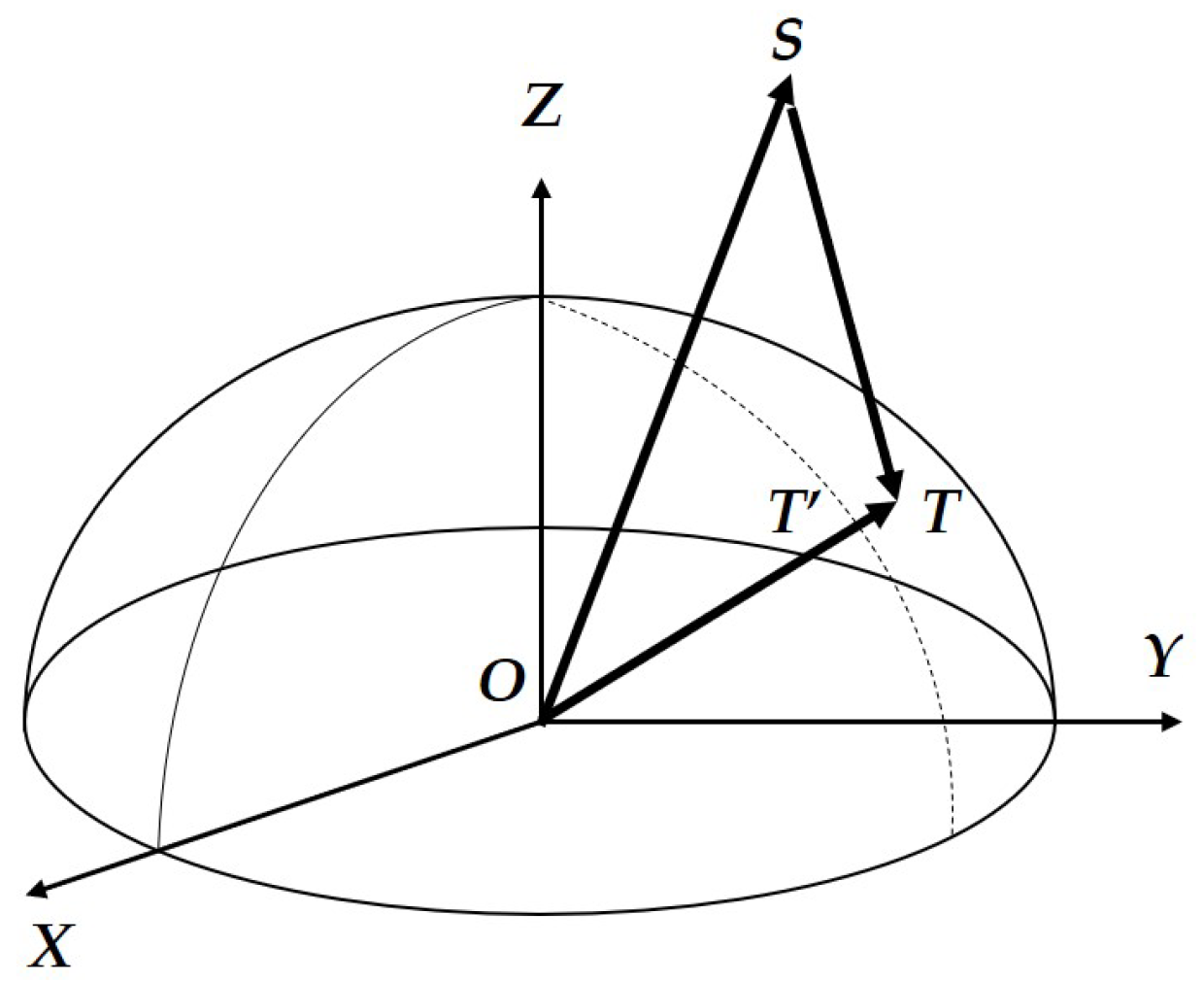
2.1. Impact of SAR Parameter Errors on the Geolocation Model

Considering Figure 1, which depicts a schematic of a SAR image acquisition in the earth centered rotating (ECR) coordinate system. S is the position of satellite. The reflection of point target T on the earth lays on $T\prime$. $TT\prime$ is the height of the target. RD geolocation model consists of three equations [38]:

$${(X_s-X_t)}^2+{(Y_s-Y_t)}^2+{(Z_s-Z_t)}^2=R^2$$

(1)

$$v_{X_s}(X_s-X_t)+v_{Y_s}(Y_s-Y_t)+v_{Z_s}(Z_s-Z_t)=-\frac{f_d\lambda R}{2}$$

(2)

$$\frac{{X_t}^2+{Y_t}^2}{{(a+h)}^2}+\frac{{Z_t}^2}{{(b+h)}^2}=1$$

(3)

where $(X_t,Y_t,Z_t)$ defines the target position, $(X_s,Y_s,Z_s)$ is the coordinate of the sensor position, $(v_{X_s},v_{Y_s},v_{Z_s})$ is the velocity vector at the respective azimuth time, R is the slant range, $f_d$ is the Doppler centroid frequency, $\lambda$ means the wavelength, a and b represents semi-major axis and semi-minor axis of reference ellipsoid, and h is the height of the target.

$(X_s,Y_s,Z_s)$ can be fitted as cubic polynomial equations from state vectors in single look complex (SLC) image parameter file as below

$$\begin{array}{c}\hfill \left\{\begin{array}{cc}{X}_s\hfill & =a_0+a_{1}t+a_2{t}^2+a_3{t}^3\hfill \\ Y_s\hfill & =b_0+b_{1}t+b_2{t}^2+b_3{t}^3\hfill \\ Z_s\hfill & =c_0+c_{1}t+c_2{t}^2+c_3{t}^3\hfill \end{array}\right.\end{array}$$

(4)

where t is the azimuth time starting at the first line of the image, and $a_0$, $a_1$, $a_2$, $a_3$, $b_0$, $b_1$, $b_2$, $b_3$, $c_0$, $c_1$, $c_2$ and $c_3$ are coefficients in the polynomials. Then $(v_{X_s},v_{Y_s},v_{Z_s})$ is the derivate of $(X_s,Y_s,Z_s)$ with respect to t.

Furthermore, $f_d$ can be presented as a function of R

$$f_d=d_0+d_1(R-R_1)+d_2{(R-R_1)}^2+d_3{(R-R_1)}^3$$

(5)

where $d_0$, $d_1$, $d_2$, $d_3$ are coefficients with respect to Doppler frequency from SLC parameter file and $R_1$ is the reference slant range of Doppler centroid.

With the RD geolocation model, $(X_t,Y_t,Z_t)$ can be conducted from pixel coordinate $(i,j)$ and other known parameters.

When it comes to the impact of SAR parameter errors on geolocation accuracy, we discuss three main parameters: orbit vectors, slant range, and target height.

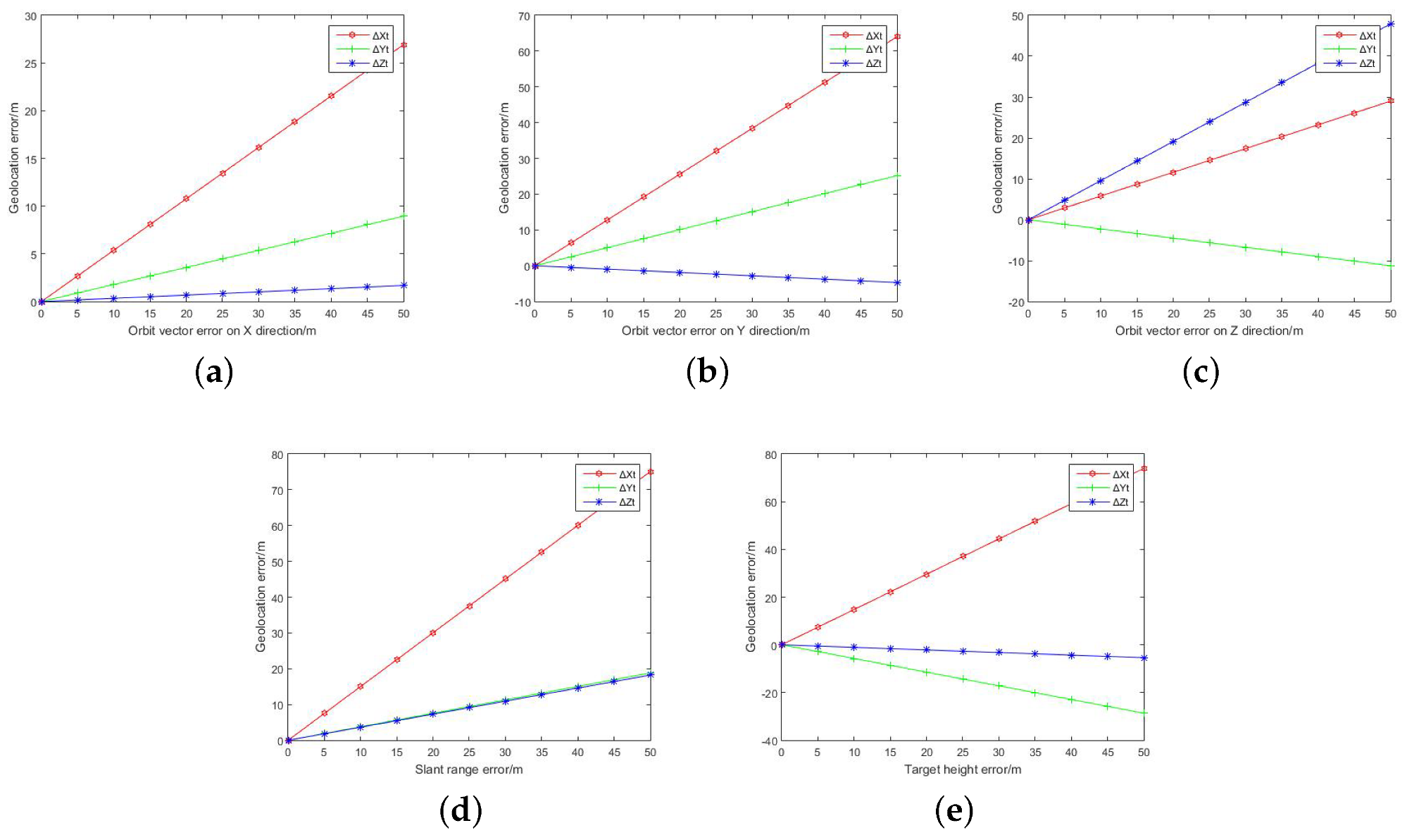
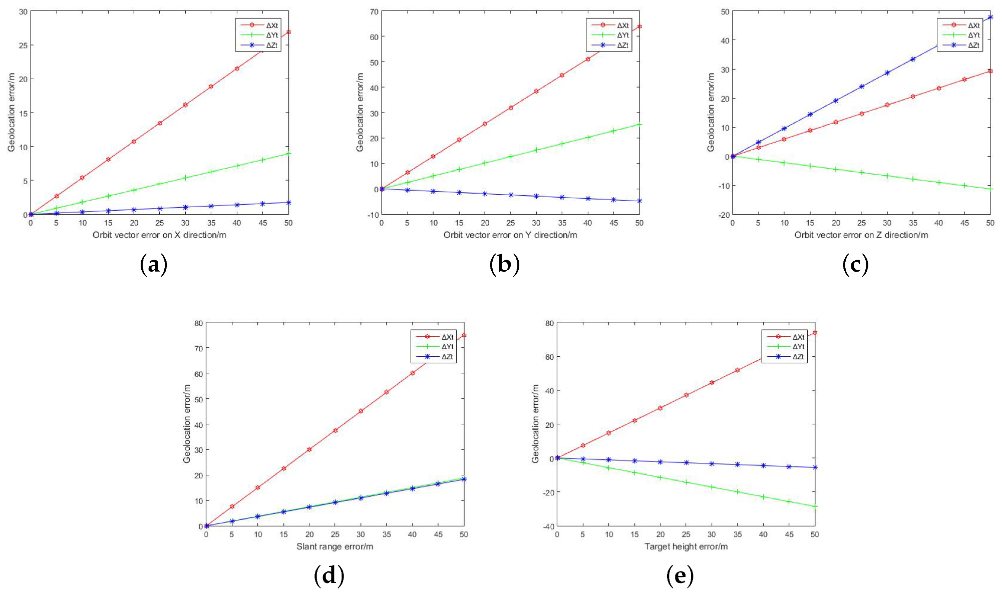
2.1.1. Orbit Vectors

The derivate of $(X_t,Y_t,Z_t)$ with reference to $(X_s,Y_s,Z_s)$ shows the relationship between target coordinate and orbit vectors. Neglecting the change of $(X_t,Y_t,Z_t)$ along with $(v_{X_s},v_{Y_s},v_{Z_s})$, the derivative of RD model Equations (1)–(3) with respect to $X_s$ can be solved as [39]

$$\begin{array}{c}\hfill \left[\begin{array}{c}\frac{\mathrm{d}{X}_t}{\mathrm{d}{X}_s}\\ \frac{\mathrm{d}{Y}_t}{\mathrm{d}{X}_s}\\ \frac{\mathrm{d}{Z}_t}{\mathrm{d}{X}_s}\end{array}\right]={\left[\begin{array}{ccc}2(X_s-X_t)& 2(Y_s-Y_t)& 2(Z_s-Z_t)\\ v_{X_s}& v_{Y_s}& v_{Z_s}\\ \frac{2X_t}{{(a+h)}^2}& \frac{2Y_t}{{(a+h)}^2}& \frac{2Z_t}{{(b+h)}^2}\end{array}\right]}^{-1}\times \left[\begin{array}{c}2(X_s-X_t)\\ v_{X_s}\\ 0\end{array}\right]\end{array}$$

(6)

The derivative of $(X_t,Y_t,Z_t)$ with respect to $Y_s$ and $Z_s$ can be solved in the same form.

2.1.2. Slant Range

Microwave signals travel through atmosphere including troposphere which causes propagation delay and affects slant range between satellite and target. The derivative of RD model equations with respect to R is

$$\begin{array}{c}\hfill \left[\begin{array}{c}\frac{\mathrm{d}{X}_t}{\mathrm{d}R}\\ \frac{\mathrm{d}{Y}_t}{\mathrm{d}R}\\ \frac{\mathrm{d}{Z}_t}{\mathrm{d}R}\end{array}\right]={\left[\begin{array}{ccc}2(X_s-X_t)& 2(Y_s-Y_t)& 2(Z_s-Z_t)\\ v_{X_s}& v_{Y_s}& v_{Z_s}\\ \frac{2X_t}{{(a+h)}^2}& \frac{2Y_t}{{(a+h)}^2}& \frac{2Z_t}{{(b+h)}^2}\end{array}\right]}^{-1}\times \left[\begin{array}{c}-2R\\ \frac{f_d\lambda }{2}\\ 0\end{array}\right]\end{array}$$

(7)

2.1.3. Target Height

DEM data is used in the process of geometric positioning when it comes to the height of target. Due to some limitations, DEM data are not exactly accurate. Then the error in target height also influences the accuracy of geolocation. The derivative of RD model equations with respect to h is

$$\begin{array}{c}\hfill \left[\begin{array}{c}\frac{\mathrm{d}{X}_t}{\mathrm{d}h}\\ \frac{\mathrm{d}{Y}_t}{\mathrm{d}h}\\ \frac{\mathrm{d}{Z}_t}{\mathrm{d}h}\end{array}\right]={\left[\begin{array}{ccc}2(X_s-X_t)& 2(Y_s-Y_t)& 2(Z_s-Z_t)\\ v_{X_s}& v_{Y_s}& v_{Z_s}\\ \frac{2X_t}{{(a+h)}^2}& \frac{2Y_t}{{(a+h)}^2}& \frac{2Z_t}{{(b+h)}^2}\end{array}\right]}^{-1}\times \left[\begin{array}{c}0\\ 0\\ \frac{2({X_t}^2+{Y_t}^2)}{{(a+h)}^3}+\frac{2{Z_t}^2}{{(b+h)}^3}\end{array}\right]\end{array}$$

(8)

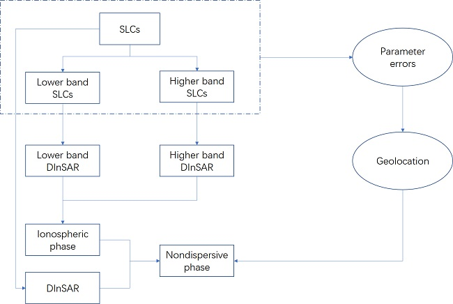
2.2. Impact of Geolocation Accuracy on the Ionospheric Phase

The interferometric phase contains several different components

$${\phi }_{int}=\frac{4\pi }{\lambda }(\mathrm{d}{R}_{topo}+\mathrm{d}{R}_{mov}+\mathrm{d}{R}_{trop}+\mathrm{d}{R}_{iono})$$

(9)

where $\mathrm{d}{R}_{topo}$ represents the topographic path delay including the flat-earth phase and the topography-related range difference from radar to target, $\mathrm{d}{R}_{mov}$ is the ground-surface displacement in radar line-of-sight (LOS) direction, and $\mathrm{d}{R}_{trop}$ and $\mathrm{d}{R}_{iono}$ are tropospheric and ionospheric delay, respectively.

The ionospheric phase delay [40] can be expressed as

$${\phi }_{iono}=\frac{4\pi K}{c{f}_0}\mathrm{d}TEC$$

(10)

where $\mathrm{d}TEC$ is the difference between the Total Electron Content (TEC) values integrated along the LOS of the master and slave radar images, K = 40.31 m${}^3$/s${}^2$ is a constant, $f_0$ is the carrier frequency of the microwave signal, and c is the speed of light.

Considering that the ionospheric path delay phase is very delicate to some necessary steps including unwrapping and spatial filtering, we take advantage of the DInSAR phase ${\phi }_{diff}$ instead of the common interferometric phase ${\phi }_{int}$ by subtracting the topographic component when using SSM. Then the DInSAR phase can be divided into two parts, and phases related to ground-surface movement and tropospheric propagation delay contribute to nondispersive phases to distinguish them from the dispersive ionospheric phase.

$${\phi }_{non-disp}=\frac{4\pi f_0}{c}(\mathrm{d}{R}_{mov}+\mathrm{d}{R}_{trop})$$

(11)

According to SSM, we divide the full spectral bands into lower and higher parts which have new radar center frequencies $f_l$ and $f_h$, respectively. The ionospheric phase [37,41] can be expressed as

$${\phi }_{iono}=\frac{f_l{f}_h}{f_0({f_h}^2-{f_l}^2)}({\phi }_l{f}_h-{\phi }_h{f}_l)$$

(12)

where ${\phi }_l$ and ${\phi }_h$ are DInSAR phases at $f_l$ and $f_h$.

According to Figure 2, where there exists geolocation error in the master image and $S_1\prime$ takes the place of $S_1$, target P is mistakenly taken at $P\prime$. $(X_s,Y_s,Z_s)$ is replaced with $({X_s}^{\prime },{Y_s}^{\prime },{Z_s}^{\prime })$ and $r_1\prime$ still meets fundamental relationships of RD imaging model Equations (1)–(3). If we define $\mathrm{d}\overrightarrow{P}$ the geolocation error, then

$${\overrightarrow{P}}^{\prime }=\overrightarrow{P}+\mathrm{d}\overrightarrow{P}$$

(13)

The topographic error phase is

$$\begin{array}{cc}\hfill {\phi }_{err}& =-\frac{4\pi }{\lambda }[(r_1^{\prime }-r_1)-(r_2^{\prime }-r_2)]\hfill \end{array}$$

(14)

According to the Doppler Equation (2), $f_d$ is the function of slant range, so

$$f_{d_1}\left(r_1\right)=-\frac{2}{\lambda }\frac{(\overrightarrow{S_1}-\overrightarrow{P})\overrightarrow{v_{S_1}}}{r_1}$$

(15)

$f_{d_2}\left(r_2\right)$ has a similar representation.

From Equation (5) and Equation (15), if $f_{d_1}$ is regarded as a intermediate variable, $r_1$ can be decided by $\overrightarrow{S_1}$, $\overrightarrow{P}$ and $\lambda$, then $r_1$ is a function of $\overrightarrow{S_1}$, $\overrightarrow{P}$ and $\lambda$

$$r_1=F_1(\overrightarrow{S_1},\overrightarrow{P},\lambda )$$

(16)

so as

$$r_2=F_2(\overrightarrow{S_2},\overrightarrow{P},\lambda )$$

(17)

Then topographic error phase can be written as

$$\begin{array}{cc}\hfill {\phi }_{err}& =-\frac{4\pi }{\lambda }[(r_1^{\prime }-r_1)-(r_2^{\prime }-r_2)]\hfill \\ \hfill & =-\frac{4\pi }{\lambda }\{[F_1({\overrightarrow{S_1}}^{\prime },\overrightarrow{P}+\mathrm{d}\overrightarrow{P},\lambda )-F_1(\overrightarrow{S_1},\overrightarrow{P},\lambda )]-[F_2({\overrightarrow{S_2}}^{\prime },\overrightarrow{P}+\mathrm{d}\overrightarrow{P},\lambda )-F_2(\overrightarrow{S_2},\overrightarrow{P},\lambda )]\}\hfill \end{array}$$

(18)

With geolocation error, according to Equation (12), ionospheric phase is in the form below

$${\phi }_{iono}^{\prime }=\frac{f_l{f}_h}{f_0({f_h}^2-{f_l}^2)}[({\phi }_l-{\phi }_{er{r}_l})f_h-({\phi }_h-{\phi }_{er{r}_h})f_l]$$

(19)

where ${\phi }_{er{r}_l}$ and ${\phi }_{er{r}_h}$ are topographic errors at lower and higher carrier frequency.

In that way, the error of the ionospheric phase with respect to geolocation error $\mathrm{d}\overrightarrow{P}$ is

$$\begin{array}{cc}{\phi }_{iono-err}\hfill & ={\phi }_{iono}^{\prime }-{\phi }_{iono}\hfill \\ \hfill & =\frac{f_l{f}_h}{f_0({f_h}^2-{f_l}^2)}\{\frac{4\pi }{{\lambda }_l}[F_1({\overrightarrow{S_1}}^{\prime },\overrightarrow{P}+\mathrm{d}\overrightarrow{P},{\lambda }_l)-F_1(\overrightarrow{S_1},\overrightarrow{P},{\lambda }_l)-F_2({\overrightarrow{S_2}}^{\prime },\overrightarrow{P}+\mathrm{d}\overrightarrow{P},{\lambda }_l)+F_2(\overrightarrow{S_2},\overrightarrow{P},{\lambda }_l)]f_h\hfill \\ \hfill & -\frac{4\pi }{{\lambda }_h}[F_1({\overrightarrow{S_1}}^{\prime },\overrightarrow{P}+\mathrm{d}\overrightarrow{P},{\lambda }_h)-F_1(\overrightarrow{S_1},\overrightarrow{P},{\lambda }_h)-F_2({\overrightarrow{S_2}}^{\prime },\overrightarrow{P}+\mathrm{d}\overrightarrow{P},{\lambda }_h)+F_2(\overrightarrow{S_2},\overrightarrow{P},{\lambda }_h)]f_l\}\hfill \end{array}$$

(20)

2.3. Impact of SAR Parameter Errors on the Ionospheric Phase

From Section 2.1 and Section 2.2, SAR parameter errors affect the accuracy of geolocation and geometric positioning error has an influence on the ionospheric phase correction. Furthermore, we determine the relationship between SAR parameter errors and the deviation of the ionospheric phase delay.

For slave SAR images, orbit polynomial equations are in the form as following

$$\begin{array}{c}\hfill \left\{\begin{array}{cc}{X}_{s_2}\hfill & =a_{02}+a_{12}t+a_{22}{t}^2+a_{32}{t}^3\hfill \\ Y_{s_2}\hfill & =b_{02}+b_{12}t+b_{22}{t}^2+b_{32}{t}^3\hfill \\ Z_{s_2}\hfill & =c_{02}+c_{12}t+c_{22}{t}^2+c_{32}{t}^3\hfill \end{array}\right.\end{array}$$

(21)

where t is the azimuth time starting at the first line of the slave image, and $a_{02}$, $a_{12}$, $a_{22}$, $a_{32}$, $b_{02}$, $b_{12}$, $b_{22}$, $b_{32}$, $c_{02}$, $c_{12}$, $c_{22}$ and $c_{32}$ are coefficients in the polynomials. Then $(v_{X_{s_2}},v_{Y_{s_2}},v_{Z_{s_2}})$ is the derivate of $(X_{s_2},Y_{s_2},Z_{s_2})$ with respect to t.

According to the RD model, the respective position of the slave satellite when imaging can be conducted with the orbit polynomial equations based on the slave SLC parameter file, after point target coordinate $(X_t,Y_t,Z_t)$ is settled.

If $(X_{s_2},Y_{s_2},Z_{s_2})$ and $(v_{X_{s_2}},v_{X_{s_2}},v_{X_{s_2}})$ are replaced with orbit polynomial Equation (21), the Doppler Equation (2) can be changed into a new form

$$\begin{array}{c}(a_{12}+2a_{22}t+3a_{32}{t}^2)(a_{02}+a_{12}t+a_{22}{t}^2+a_{32}{t}^3-X_t)+\hfill \\ (b_{12}+2b_{22}t+3b_{32}{t}^2)(b_{02}+b_{12}t+b_{22}{t}^2+b_{32}{t}^3-Y_t)+\hfill \\ (c_{12}+2c_{22}t+3c_{32}{t}^2)(c_{02}+c_{12}t+c_{22}{t}^2+c_{32}{t}^3-Z_t)\hfill \\ =-\frac{f_d\lambda }{2}\sqrt{{(a_{02}+a_{12}t+a_{22}{t}^2+a_{32}{t}^3-X_t)}^2+{(b_{02}+b_{12}t+b_{22}{t}^2+b_{32}{t}^3-Y_t)}^2+{(c_{02}+c_{12}t+c_{22}{t}^2+c_{32}{t}^3-Z_t)}^2}\hfill \end{array}$$

(22)

Based on the new Doppler Equation (22), azimuth time t in slave SLC image is the function of $(X_t,Y_t,Z_t)$ and $\lambda$ when $f_d$ is calculated through SLC parameter file, so it can be expressed as

$$t=g(X_t,Y_t,Z_t,\lambda )$$

(23)

For slant range between slave satellite and target

$$\begin{array}{cc}\hfill r_2& =\sqrt{{(X_{s_2}-X_t)}^2+{(Y_{s_2}-Y_t)}^2+{(Z_{s_2}-Z_t)}^2}\hfill \\ \hfill & =\sqrt{{(a_{02}+a_{12}t+a_{22}{t}^2+a_{32}{t}^3-X_t)}^2+{(b_{02}+b_{12}t+b_{22}{t}^2+b_{32}{t}^3-Y_t)}^2+{(c_{02}+c_{12}t+c_{22}{t}^2+c_{32}{t}^3-Z_t)}^2}\hfill \end{array}$$

(24)

Like Equation (23), $r_2$ can be regarded as a function of t, $(X_t,Y_t,Z_t)$ and $\lambda$

$$r_2=w(t,X_t,Y_t,Z_t,\lambda )$$

(25)

2.3.1. Orbit Vectors from Master SLC Parameter File

The derivative of slave azimuth time t with respect to $X_t$ is

$$\frac{\mathrm{d}t}{\mathrm{d}{X}_s}=\frac{\mathrm{d}g}{\mathrm{d}{X}_t}\frac{\mathrm{d}{X}_t}{\mathrm{d}{X}_s}+\frac{\mathrm{d}g}{\mathrm{d}{Y}_t}\frac{\mathrm{d}{Y}_t}{\mathrm{d}{X}_s}+\frac{\mathrm{d}g}{\mathrm{d}{Z}_t}\frac{\mathrm{d}{Z}_t}{\mathrm{d}{X}_s}$$

(26)

where $\frac{\mathrm{d}{X}_t}{\mathrm{d}{X}_s}$, $\frac{\mathrm{d}{Y}_t}{\mathrm{d}{X}_s}$, $\frac{\mathrm{d}{Z}_t}{\mathrm{d}{X}_s}$ have already been conducted in Section 2.1.

$\frac{\mathrm{d}t}{\mathrm{d}{Y}_s}$ and $\frac{\mathrm{d}t}{\mathrm{d}{Z}_s}$ have similar form as $\frac{\mathrm{d}t}{\mathrm{d}{X}_s}$.

Then the derivates of slave slant range with reference to different factors can be conducted according to Equation (25).

Combined with derivates of t

$$\frac{\mathrm{d}{r}_2}{\mathrm{d}{X}_s}=\frac{\mathrm{d}{r}_2}{\mathrm{d}t}\frac{\mathrm{d}t}{\mathrm{d}{X}_s}+\frac{\mathrm{d}{r}_2}{\mathrm{d}{X}_t}\frac{\mathrm{d}{X}_t}{\mathrm{d}{X}_s}+\frac{\mathrm{d}{r}_2}{\mathrm{d}{Y}_t}\frac{\mathrm{d}{Y}_t}{\mathrm{d}{X}_s}+\frac{\mathrm{d}{r}_2}{\mathrm{d}{Z}_t}\frac{\mathrm{d}{Z}_t}{\mathrm{d}{X}_s}$$

(27)

So as $\frac{\mathrm{d}{r}_2}{\mathrm{d}{Y}_s}$ and $\frac{\mathrm{d}{r}_2}{\mathrm{d}{Z}_s}$.

Combined with Equation (20) from Section 2.2, the derivate of the ionospheric phase with respect to $X_s$ is

$$\frac{\mathrm{d}{\phi }_{iono}}{\mathrm{d}{X}_s}=\frac{4\pi {f_l}^2{f_h}^2}{c{f}_0({f_h}^2-{f_l}^2)}[\frac{\mathrm{d}{r}_2\left({\lambda }_h\right)}{\mathrm{d}{X}_s}-\frac{\mathrm{d}{r}_2\left({\lambda }_l\right)}{\mathrm{d}{X}_s}]$$

(28)

In the same way

$$\frac{\mathrm{d}{\phi }_{iono}}{\mathrm{d}{Y}_s}=\frac{4\pi {f_l}^2{f_h}^2}{c{f}_0({f_h}^2-{f_l}^2)}[\frac{\mathrm{d}{r}_2\left({\lambda }_h\right)}{\mathrm{d}{Y}_s}-\frac{\mathrm{d}{r}_2\left({\lambda }_l\right)}{\mathrm{d}{Y}_s}]$$

(29)

$$\frac{\mathrm{d}{\phi }_{iono}}{\mathrm{d}{Z}_s}=\frac{4\pi {f_l}^2{f_h}^2}{c{f}_0({f_h}^2-{f_l}^2)}[\frac{\mathrm{d}{r}_2\left({\lambda }_h\right)}{\mathrm{d}{Z}_s}-\frac{\mathrm{d}{r}_2\left({\lambda }_l\right)}{\mathrm{d}{Z}_s}]$$

(30)

2.3.2. Master Slant Range

Combined with the derivative of azimuth time t of slave SLC image with respect to the slant range of master image $r_1$, and the slave slant range $r_2$ with reference to the master slant range $r_1$, then

$$\begin{array}{cc}\hfill \frac{\mathrm{d}{\phi }_{iono}}{\mathrm{d}{r}_1}& =\frac{f_l{f}_h}{f_0({f_h}^2-{f_l}^2)}[\frac{4\pi }{{\lambda }_l}(1-\frac{\mathrm{d}{r}_2\left({\lambda }_l\right)}{\mathrm{d}{r}_1})f_h-\frac{4\pi }{{\lambda }_h}(1-\frac{\mathrm{d}{r}_2\left({\lambda }_h\right)}{\mathrm{d}{r}_1})f_l]\hfill \\ \hfill & =\frac{4\pi {f_l}^2{f_h}^2}{c{f}_0({f_h}^2-{f_l}^2)}[\frac{\mathrm{d}{r}_2\left({\lambda }_h\right)}{\mathrm{d}{r}_1}-\frac{\mathrm{d}{r}_2\left({\lambda }_l\right)}{\mathrm{d}{r}_1}]\hfill \end{array}$$

(31)

2.3.3. Target Height

Combined with the derivative of azimuth time t of slave SLC image with respect to the height of target h, and the slave slant range $r_2$ with reference to the height of target h, then

$$\frac{\mathrm{d}{\phi }_{iono}}{\mathrm{d}h}=\frac{4\pi {f_l}^2{f_h}^2}{c{f}_0({f_h}^2-{f_l}^2)}[\frac{\mathrm{d}{r}_2\left({\lambda }_h\right)}{\mathrm{d}h}-\frac{\mathrm{d}{r}_2\left({\lambda }_l\right)}{\mathrm{d}h}]$$

(32)

3. Numerical Simulation

3.1. Impact of SAR Parameter Errors on the Geolocation Model

To analyze the specific relationship between SAR system parameter errors and the deviation of the target coordinate, we simulate a point target from ALOS PALSAR-1 interferogram on 20080131 and 20080317 and another interferogram on 20100623 and 20100808 over Antofagasta, Chile.

In the first case on 20080131 and 20080317, the master slant range of this point is 876,845.8487 m, the respective azimuth Coordinated Universal Time (UTC) is 13,365.6580 s and the target height is 906.0579 m. The error equation of SAR geolocation is given in Section 2.1, so the impact can be estimated when there exist errors on orbit vectors, slant range, and target height.

Cubic polynomial Equation (4) are calculated with orbit vectors from the parameter file on 20080131.

$$\left\{\begin{array}{c}{X}_s=-968896044.2932+203773.1547\times t-14.1331\times t^2+3.2323\times {10}^{-4}\times t^3\hfill \\ Y_s=-915139813.1383+257717.5799\times t-23.0514\times t^2+6.6268\times {10}^{-4}\times t^3\hfill \\ Z_s=3223643924.2163-716260.2857\times t+52.4879\times t^2-0.0013\times t^3\hfill \end{array}\right.$$

(33)

where t is UTC at azimuth direction.

Firstly, the error of 5 m, 10 m, 15 m, …, 45 m, 50 m are added independently in the X axis of orbit vectors, the coordinate of point target $(X_t,Y_t,Z_t)$ is calculated and we get the geolocation error in three different directions compared with the exact coordinate.

In the same way, errors are added in Y and Z directions of orbit vectors, slant range R and target height h, and the respective geolocation errors are calculated. Then the geolocation error in three directions of orbit vectors, slant range and target height are plotted in Figure 3.

In Figure 3, the horizontal axis shows the error added in different factors, and the vertical axis is geolocation error. The red line represents error in X direction of the target coordinate, the green and blue ones are errors in the Y and Z components.

According to Figure 3a, geolocation error in different directions all grow with X orbit error, and they are correlated in a linear relationship. The impact on X axis of geolocation error is about three times of that on the Y axis. We calculate the derivates of geolocation with respect to $X_s$ and other components of orbit vectors, slant range and target height considering the form of matric with Equations (6)–(8). The derivates are shown in

Table 1. The derivates of geolocation with respect to SAR parameters on 20080131 and 20080317.

SAR Parameters	Derivate of ${\mathit{X}}_{\mathit{t}}$	Derivate of ${\mathit{Y}}_{\mathit{t}}$	Derivate of ${\mathit{Z}}_{\mathit{t}}$
$X_s$	0.5384	0.1789	0.0338
$Y_s$	1.2801	0.5040	−0.0936
$Z_s$	0.5803	−0.2248	0.9576
R	1.5015	0.3768	0.3633
h	1.4793	−0.5732	−0.1082

.

The values of derivates agree with the gradients of lines shown in Figure 3.

In another case on 20100623 and 20100808, the master slant range of this point is 876,845.9523 m, the respective azimuth time of UTC is 13,470.1155 s and the target height is 1131.8140 m. Cubic polynomial Equation (4) are calculated with orbit vectors from the parameter file on 20100623.

$$\left\{\begin{array}{c}{X}_s=-1006468593.0374+210256.2397\times t-14.4909\times t^2+3.2947\times {10}^{-4}\times t^3\hfill \\ Y_s=-904280697.1649+254049.3536\times t-22.6228\times t^2+6.4677\times {10}^{-4}\times t^3\hfill \\ Z_s=3318569557.1120-731387.9905\times t+53.1749\times t^2-0.0013\times t^3\hfill \end{array}\right.$$

(34)

When the same errors are added independently in the X, Y and Z directions of orbit vectors, slant range R and target height h, the respective geolocation errors are calculated. The geolocation error in three directions of orbit vectors, slant range and target height are plotted in Figure 4.

The derivates of geolocation with respect to different parameters are calculated shown in

Table 2. The derivates of geolocation with respect to SAR parameters on 20100623 and 20100808.

SAR Parameters	Derivate of ${\mathit{X}}_{\mathit{t}}$	Derivate of ${\mathit{Y}}_{\mathit{t}}$	Derivate of ${\mathit{Z}}_{\mathit{t}}$
$X_s$	0.5376	0.1785	0.0349
$Y_s$	1.2777	0.5066	−0.0965
$Z_s$	0.5860	−0.2263	0.9558
R	1.5016	0.3765	0.3638
h	1.4798	−0.5714	−0.1117

.

The values of derivates from Table 2 agree with the slopes of lines shown in Figure 4.

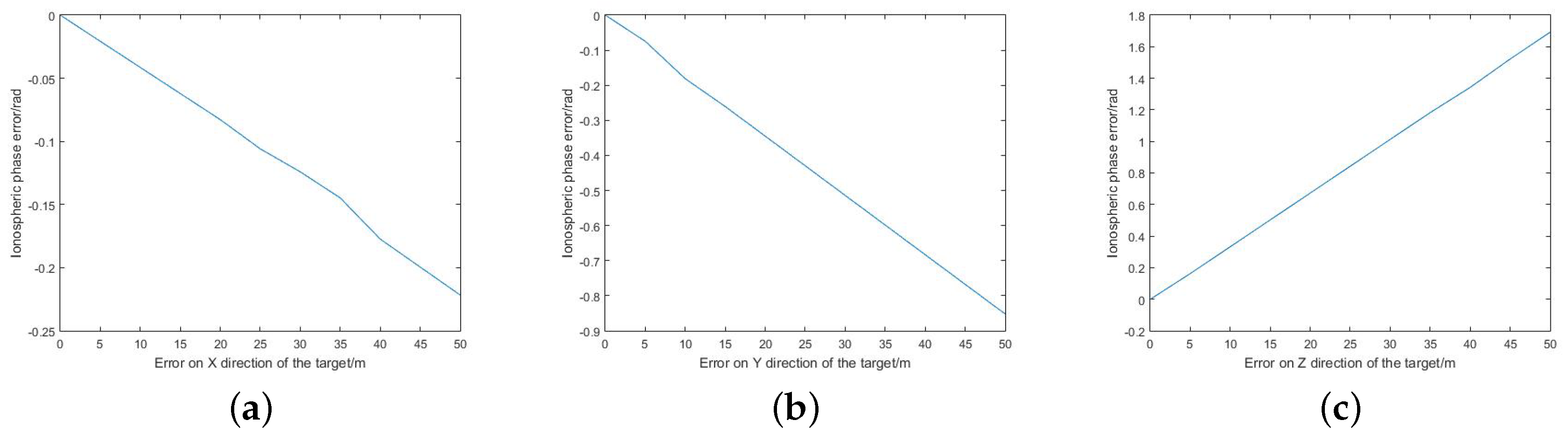
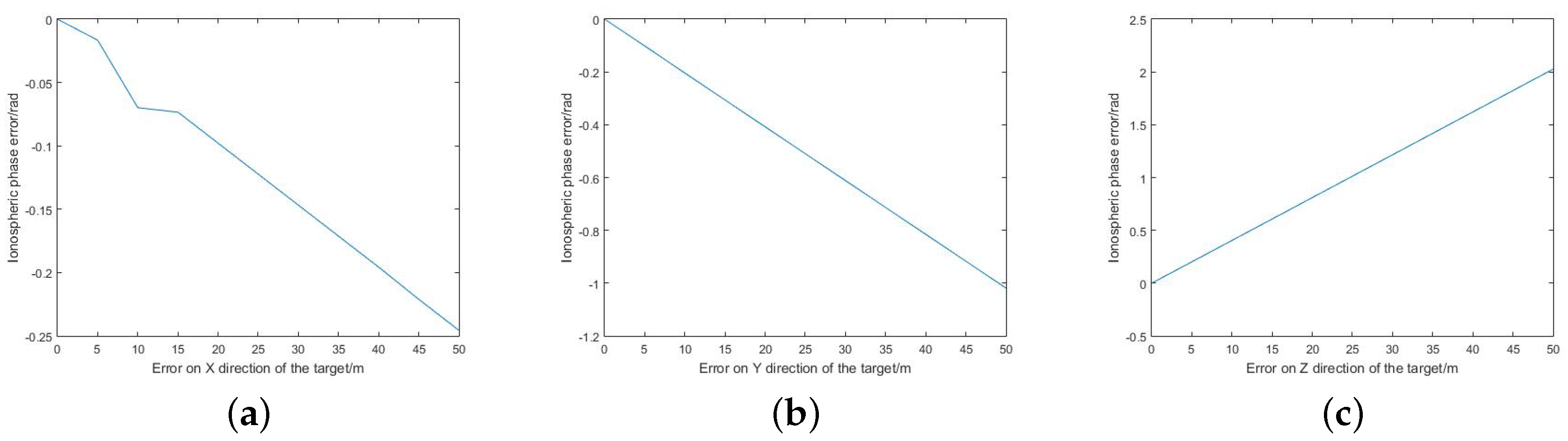
3.2. Impact of Geolocation Accuracy on the Ionospheric Phase

In order to estimate the relationship between geolocation accuracy and ionospheric delay, the error is added in different directions of the target coordinate. Then the phases of the ionosphere are calculated and compared with the exact value without geolocation error.

We add 5 m, 10 m, 15 m, …, 45 m, 50 m errors in different directions of target in the case on 20080131 and 20080317, the differences between the new ionospheric phase and the exact value are calculated. Furthermore, the results are plotted in Figure 5.

From Figure 5a, the ionospheric phase error grows with X axis of geolocation error, and it is linearly related to the error in X direction with a slope around −0.0044 rad/m. Then the ionospheric phase error is correlated with the geolocation error in Y direction in a linear relationship with a gradient around −0.0171 rad/m and is linearly to the error in Z direction with a slope around 0.0339 rad/m according to Figure 5b,c.

Then we add the same errors in different directions of target in the case on 20100623 and 20100808, the differences between the new ionospheric phase and the exact value are calculated. Furthermore, the results are plotted in Figure 6.

From Figure 6a, the ionospheric phase error grows with the geolocation error on X axis, and it is linearly related to the error in X direction with a slope around −0.0048 rad/m. Then the ionospheric phase error is correlated with the geolocation error in Y direction in a linear relationship with a gradient around −0.0204 rad/m and is linearly to the error in Z direction with a slope around 0.0405 rad/m according to Figure 6b,c.

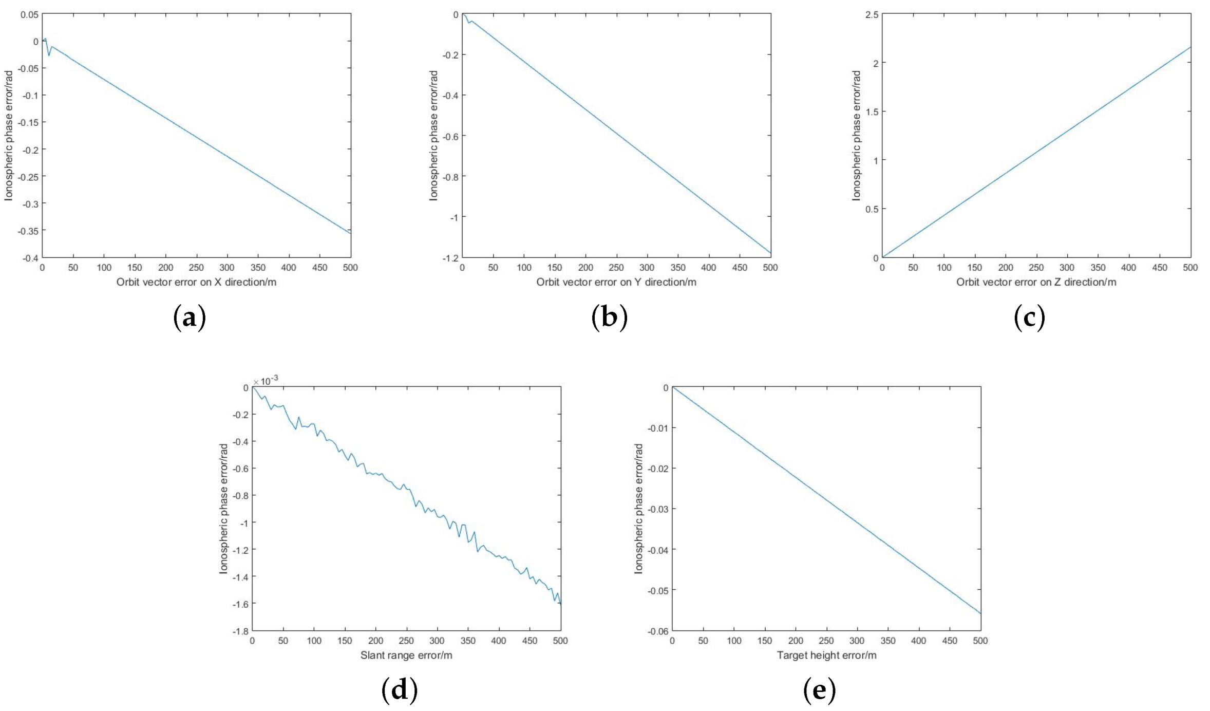
3.3. Impact of SAR Parameter Errors on the Ionospheric Phase

In order to determine the relationship between SAR parameter errors and the deviation of the ionospheric phase, the results in Section 3.1 and Section 3.2. can be considered into a combination.

For the first case, cubic polynomial equations are calculated with orbit vectors from parameter file on 20080317 with Equation (21).

$$\left\{\begin{array}{c}{X}_{s_2}=-932207141.0991+196180.9423\times t-13.6073\times t^2+3.1101\times {10}^{-4}\times t^3\hfill \\ Y_{s_2}=-977378076.6340+272168.2696\times t-24.1906\times t^2+6.9304\times {10}^{-4}\times t^3\hfill \\ Z_{s_2}=3163524048.9463-704835.3431\times t+51.7836\times t^2-1.2549\times {10}^{-3}\times t^3\hfill \end{array}\right.$$

(35)

We add 5 m, …, 500 m errors in different directions of orbit vectors from master image, master slant range and target height, then the ionospheric phase errors are plotted in Figure 7.

The phase error is in a linear relationship with orbit error in X direction at around $-6.2229\times {10}^{-4}$ rad/m. Furthermore, slopes are about $-0.0020$ rad/m, $0.0036$ rad/m, $-5.2607\times {10}^{-5}$ rad/m and $-1.0073\times {10}^{-4}$ rad/m for errors in Y and Z direction, master slant range and target height.

Then cubic polynomial equations according to orbit vectors from parameter file on 20100808 are

$$\left\{\begin{array}{c}{X}_{s_2}=-961770440.0508+200835.5303\times t-13.8263\times t^2+3.1376\times {10}^{-4}\times t^3\hfill \\ Y_{s_2}=-993773145.4944+274356.9804\times t-24.1761\times t^2+6.8673\times {10}^{-4}\times t^3\hfill \\ Z_{s_2}=3252779016.9887-718459.2228\times t+52.3394\times t^2-1.2579\times {10}^{-3}\times t^3\hfill \end{array}\right.$$

(36)

The respective ionospheric phase errors are plotted in Figure 8.

The phase error is in a linear relationship with orbit error in X direction at around $-7.1101\times {10}^{-4}$ rad/m. Furthermore, slopes are about $-0.0024$ rad/m, $0.0043$ rad/m, $-3.0637\times {10}^{-6}$ rad/m and $-1.1168\times {10}^{-4}$ rad/m for errors in Y and Z direction, master slant range and target height.

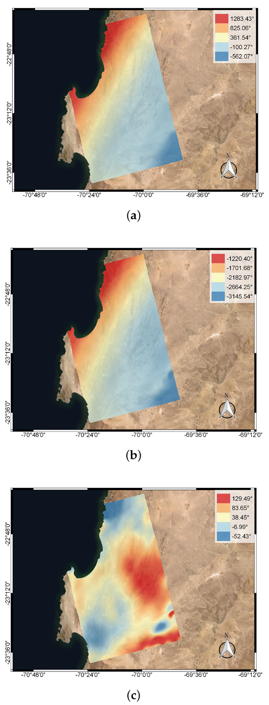
4. Experimental Results

We select an area (track 104, frames 6710–6720) from ALOS PALSAR-1 interferogram on 20080131 and 20080317 and another area (track 104, frame 6710) on 20100623 and 20100808 over Antofagasta in Chile, to demonstrate the impact of SAR parameter errors on the ionospheric correction based on SSM.

In the first case on 20080131 and 20080317, the Doppler centroid frequency of the master SLC image is 92.12 Hz, the baseline is 914.12 m and the range of elevation is 62.41~1572.74 m. We use SSM to estimate the ionospheric phase delay and the corrected DInSAR phase (also nondispersive phase according to SSM). The correction results are shown in Figure 9.

Where there exists an error in the Doppler centroid frequency, according to Equation (2), the coordinate of the target will be inaccurate. It leads to geolocation error and affects the ionospheric correction in the end. We add an error around 90 Hz to the Doppler frequency of the master SLC image, and then use SSM to calculate the ionospheric phase and the corrected DInSAR phase, which are shown in Figure 10. We assume the corrected DInSAR phase without any parameter error from Figure 9c as truth and compute the difference between the corrected DInSAR phase with Doppler frequency error in Figure 10b and the corrected DInSAR phase without parameter error. The difference phase is shown in Figure 10c.

The baseline of two sensors is determined by the orbit vectors of SLCs. The error in orbit vectors results in baseline error, and then baseline error influences the ionospheric correction. We add an error around 0.20 m to the baseline of the interferogram on 20080131 and 20080317 and use SSM to calculate the ionospheric phase and the corrected DInSAR phase. The ionospheric correction result is shown in Figure 11. The difference between the corrected DInSAR phase with baseline error and the corrected DInSAR phase without parameter error from Figure 9c is shown in Figure 11c. The linear fringes in Figure 11c show the features of orbital error.

We add an error around 925.60 m to the height of the area and use SSM to calculate the ionospheric phase and the corrected DInSAR phase. The ionospheric correction result and the corrected phase difference are shown in Figure 12.

In the second case on 20100623 and 20100808, the Doppler centroid frequency of the master SLC image is 110.08 Hz, the baseline is 266.05 m and the range of elevation is 87.14~1462.61 m. We use SSM to estimate the ionospheric phase delay and the corrected DInSAR phase. The correction results are shown in Figure 13.

We add an error around 110 Hz to the Doppler frequency of the master SLC image, the ionospheric correction result is shown in Figure 14 and the difference between the corrected DInSAR phase with Doppler frequency error and the corrected DInSAR phase without parameter error from Figure 13c is shown in Figure 14c.

We add an error around 0.01 m to the baseline of the interferogram on 20100623 and 20100808, the ionospheric correction result and the corrected phase difference are shown in Figure 15.

We add an error around 942.01 m to the height of the area, the ionospheric correction result and the corrected phase difference are shown in Figure 16.

5. Discussion

To discuss how SAR parameter errors affect ionospheric phase correction, we build a model to analyze the impact of SAR parameter errors on the ionospheric correction based on SSM, then do numerical simulations to testify that the deviation of the ionospheric phase has a linear relationship with SAR parameter errors. In the end, we do experiments with ionospheric disturbed data by SSM to get the ionospheric phase and the corrected DInSAR phase.

In Section 4, we assume the corrected DInSAR phase without parameter errors as truth. Then we add error to the SAR parameters of the same data, use SSM to get the ionospheric phase and the corrected DInSAR phase respectively when SAR parameter errors exist.

Comparing the corrected DInSAR phase with parameter errors and the corrected DInSAR phase without parameter errors reveals that the impact of SAR parameter errors on the ionospheric correction is significant. To quantifying the difference between the corrected DInSAR phase with parameter errors and the corrected DInSAR phase without parameter errors, we assume the corrected DInSAR phase without parameter errors as truth and compute the deviation of the corrected DInSAR phase with SAR parameter errors using RMSE given as

$$RMSE=\sqrt{\frac{{\sum }_{i=1}^N{({{\phi }_i}^{err}-{{\phi }_i}^0)}^2}{N}}$$

(37)

where ${{\phi }_i}^{err}$ and ${{\phi }_i}^0$ represent the corrected DInSAR phase with parameter errors and the corrected DInSAR phase without parameter errors, respectively, at the ith DInSAR pixel, and N is the number of pixels in the DInSAR image.

For the first case on 20080131 and 20080317, according to Equation (37), the RMSE between the corrected DInSAR phase with Doppler frequency error and the corrected DInSAR phase without parameter errors is 269.29${}^{\circ }$. As we know, the wavelength of ALOS PALSAR-1 is about 23.26 cm. Then the value of RMSE is equal to 17.40 cm in distance. In the same way, we calculate the RMSE between the corrected DInSAR phase with different parameter errors and the corrected DInSAR phase without parameter errors in distance and show the values in

Table 3. The root mean square error (RMSE) between the corrected DInSAR phase with different parameter errors and the corrected DInSAR phase without parameter errors in distance on 20080131 and 20080317.

Parameter Error	Doppler Frequency (90 Hz)	Baseline (0.20 m)	Height (925.60 m)
RMSE/cm	17.40	5.22	9.29

.

For the second case on 20100623 and 20100808, the values of RMSE are calculated in the same way and shown in

Table 4. The RMSE between the corrected DInSAR phase with different parameter errors and the corrected DInSAR phase without parameter errors in distance on 20100623 and 20100808.

Parameter Error	Doppler Frequency (110 Hz)	Baseline (0.01 m)	Height (942.01 m)
RMSE/cm	12.69	2.00	1.33

.

The values of RMSE between the corrected DInSAR phase with parameter errors and the corrected DInSAR phase without parameter errors vary from centimeter to decimeter level with the L-band data. It demonstrates that the ionospheric correction is sensitive to SAR parameter errors. The impact of SAR parameter errors on the ionospheric correction based on SSM is significant. Furthermore, the effectiveness of SSM can be improved when SAR parameters are accurately estimated.

6. Conclusions

This paper discusses the relationship between SAR parameter errors and the deviation of the ionospheric phase in the process of separating the ionospheric and the nondispersive phase with lower and higher sub-band interferograms. We built a model by calculating the derivates of geolocation with respect to parameter errors on the basis of the RD imaging model as well as getting the impact of target coordinate error on the ionospheric phase delay. Then we did numerical simulation to testify the impact of SAR parameter errors on the ionospheric correction. We evaluated the exact influence and concluded that the deviation of the ionospheric phase is linearly related to SAR parameter errors.

Through experiments on two interferograms with L-band data acquired from ALOS PALSAR-1 satellite in Chile, we calculated the ionospheric phase delay and the corrected DInSAR phase with SSM. Considering Doppler frequency error, baseline error and height error, the corrected DInSAR images with different parameter errors were presented in this article and showed that the SAR parameter errors significantly affected the performance of ionospheric correction. We computed the deviation of ionospheric correction results with parameter errors. The values of RMSE between the corrected DInSAR phase with parameter errors and the corrected DInSAR phase without parameter errors varied from centimeter to decimeter level in distance demonstrating the delicateness of the ionospheric correction to SAR parameter errors. Furthermore, the correction effectiveness of SSM could be improved when SAR parameters were accurately estimated.

References

1. Bamler, R.; Hartl, P. Synthetic aperture radar interferometry. Inverse Probl. 1998, 14, R1–R54. [Google Scholar] [CrossRef]
2. Amelung, F.; Yun, S.H.; Walter, T.R.; Segall, P.; Kim, S.W. Stress control of deep rift intrusion at Mauna Loa volcano, Hawaii. Science 2007, 316, 1026–1030. [Google Scholar] [CrossRef] [PubMed]
3. Hooper, A.; Bekaert, D.; Spaans, K.; Arikan, M. Recent advances in SAR interferometry time series analysis for measuring crustal deformation. Tectonophysics 2012, 514, 1–13. [Google Scholar] [CrossRef]
4. Lu, Z.; Kwoun, O.; Rykhus, R. Interferometric synthetic aperture radar (InSAR): Its past, present and future. Photogramm. Eng. Remote Sens. 2007, 73, 217–221. [Google Scholar]
5. Massonnet, D.; Feigl, K.L. Radar interferometry and its application to changes in the earth’s surface. Rev. Geophys. 1998, 36, 441–500. [Google Scholar] [CrossRef] [Green Version]
6. Baer, G.; Magen, Y.; Nof, R.N.; Raz, E.; Lyakhovsky, V.; Shalev, E. InSAR Measurements and Viscoelastic Modeling of Sinkhole Precursory Subsidence: Implications for Sinkhole Formation, Early Warning, and Sediment Properties. J. Geophys. Res.-Earth Surf. 2018, 123, 678–693. [Google Scholar] [CrossRef]
7. Berardino, P.; Fornaro, G.; Lanari, R.; Sansosti, E. A new algorithm for surface deformation monitoring based on small baseline differential SAR interferograms. IEEE Trans. Geosci. Remote Sens. 2002, 40, 2375–2383. [Google Scholar] [CrossRef] [Green Version]
8. Lv, X.; Yazici, B.; Zeghal, M.; Bennett, V.; Abdoun, T. Joint-Scatterer Processing for Time-Series InSAR. IEEE Trans. Geosci. Remote Sens. 2014, 52, 7205–7221. [Google Scholar] [CrossRef]
9. Yun, Y.; Lv, X.; Fu, X.; Xue, F. Application of Spaceborne Interferometric Synthetic Aperture Radar to Geohazard Monitoring. J. Radars 2020, 9, 73–85. [Google Scholar]
10. Bekaert, D.P.S.; Hooper, A.; Wright, T.J. A spatially variable power law tropospheric correction technique for InSAR data. J. Geophys. Res.-Solid Earth 2015, 120, 1345–1356. [Google Scholar] [CrossRef]
11. Bekaert, D.P.S.; Walters, R.J.; Wright, T.J.; Hooper, A.J.; Parker, D.J. Statistical comparison of InSAR tropospheric correction techniques. Remote Sens. Environ. 2015, 170, 40–47. [Google Scholar] [CrossRef] [Green Version]
12. Li, Z.W.; Ding, X.L.; Liu, G. Modeling atmospheric effects on InSAR with meteorological and continuous GPS observations: Algorithms and some test results. J. Atmos. Solar-Terr. Phys. 2004, 66, 907–917. [Google Scholar] [CrossRef]
13. Webley, P.W.; Bingley, R.M.; Dodson, A.H.; Wadge, G.; Waugh, S.J.; James, I.N. Atmospheric water vapour correction to InSAR surface motion measurements on mountains: Results from a dense GPS network on Mount Etna. Phys. Chem. Earth 2002, 27, 363–370. [Google Scholar] [CrossRef]
14. Yu, C.; Li, Z.; Penna, N.T. Interferometric synthetic aperture radar atmospheric correction using a GPS-based iterative tropospheric decomposition model. Remote Sens. Environ. 2018, 204, 109–121. [Google Scholar] [CrossRef]
15. Yu, C.; Li, Z.; Penna, N.T.; Crippa, P. Generic Atmospheric Correction Model for Interferometric Synthetic Aperture Radar Observations. J. Geophys. Res.-Solid Earth 2018, 123, 9202–9222. [Google Scholar] [CrossRef]
16. Foster, J.; Brooks, B.; Cherubini, T.; Shacat, C.; Businger, S.; Werner, C.L. Mitigating atmospheric noise for InSAR using a high resolution weather model. Geophys. Res. Lett. 2006, 33. [Google Scholar] [CrossRef]
17. Jolivet, R.; Agram, P.S.; Lin, N.Y.; Simons, M.; Doin, M.P.; Peltzer, G.; Li, Z. Improving InSAR geodesy using Global Atmospheric Models. J. Geophys. Res.-Solid Earth 2014, 119, 2324–2341. [Google Scholar] [CrossRef]
18. Jolivet, R.; Grandin, R.; Lasserre, C.; Doin, M.P.; Peltzer, G. Systematic InSAR tropospheric phase delay corrections from global meteorological reanalysis data. Geophys. Res. Lett. 2011, 38. [Google Scholar] [CrossRef] [Green Version]
19. Shimada, M. Correction of the satellite’s state vector and the atmospheric excess path delay in SAR interferometry—Application to surface deformation detection. In Proceedings of the IEEE 2000 International Geoscience and Remote Sensing Symposium, Taking the Pulse of the Planet: The Role of Remote Sensing in Managing the Environment, Honolulu, HI, USA, 24–28 July 2000; pp. 2236–2238. [Google Scholar]
20. Shimada, M.; Minamisawa, M.; Isoguchi, O.; Ieee, I. Correction of atmospheric excess path delay appeared in repeat-pass SAR interferometry using objective analysis data. In Proceedings of the IGARSS 2001, Scanning the Present and Resolving the Future, IEEE 2001 International Geoscience and Remote Sensing Symposium (Cat. No.01CH37217), Sydney, NSW, Australia, 9–13 July 2001; pp. 2052–2054. [Google Scholar]
21. Gray, A.L.; Mattar, K.E.; Sofko, G. Influence of ionospheric electron density fluctuations on satellite radar interferometry. Geophys. Res. Lett. 2000, 27, 1451–1454. [Google Scholar] [CrossRef]
22. Mattar, K.E.; Gray, A.L. Reducing ionospheric electron density errors in satellite radar interferometry applications. Can. J. Remote Sens. 2002, 28, 593–600. [Google Scholar] [CrossRef]
23. Rignot, E.J.M. Effect of Faraday rotation on L-band interferometric and polarimetric synthetic-aperture radar data. IEEE Trans. Geosci. Remote Sens. 2000, 38, 383–390. [Google Scholar] [CrossRef] [Green Version]
24. Rosen, P.A.; Hensley, S.; Chen, C. Measurement and Mitigation of the Ionosphere in L-band Interferometric SAR Data. In Proceedings of the 2010 Ieee Radar Conference, Washington, DC, USA, 10–14 May 2010; pp. 1459–1463. [Google Scholar] [CrossRef]
25. Brcic, R.; Parizzi, A.; Eineder, M.; Bamler, R.; Meyer, F. Estimation and compensation of ionospheric delay for sar interferometry. In Proceedings of the 2010 Ieee International Geoscience and Remote Sensing Symposium, Honolulu, HI, USA, 25–30 July 2010; pp. 2908–2911. [Google Scholar] [CrossRef]
26. Gomba, G.; Gonzalez, F.R.; De Zan, F. Ionospheric Phase Screen Compensation for the Sentinel-1 TOPS and ALOS-2 ScanSAR Modes. IEEE Trans. Geosci. Remote Sens. 2017, 55, 223–235. [Google Scholar] [CrossRef]
27. Gomba, G.; Parizzi, A.; De Zan, F.; Eineder, M.; Bamler, R. Toward Operational Compensation of Ionospheric Effects in SAR Interferograms: The Split-Spectrum Method. IEEE Trans. Geosci. Remote Sens. 2016, 54, 1446–1461. [Google Scholar] [CrossRef] [Green Version]
28. Schubert, A.; Small, D.; Miranda, N.; Geudtner, D.; Meier, E. Sentinel-1A Product Geolocation Accuracy: Commissioning Phase Results. Remote Sens. 2015, 7, 9431–9449. [Google Scholar] [CrossRef] [Green Version]
29. Dong, X.T.; Zhao, Y.H.; Yue, X.J.; Han, C.M. An Accurate Co-registration Method for Airborne Repeatpass InSAR. In Proceedings of the 2017 International Conference on Sustainable Development on Energy and Environment Protection, Yichang, China, 28–30 July 2017; Volume 86. [Google Scholar] [CrossRef] [Green Version]
30. Johnsen, H.; Lauknes, L.; Guneriussen, T. Geocoding of fast-delivery ers-1 sar image mode product using dem data. Int. J. Remote Sens. 1995, 16, 1957–1968. [Google Scholar] [CrossRef]
31. Liu, X.; Ma, H.; Sun, W. Study on the geolocation algorithm of space-borne SAR image. In Advances in Machine Vision, Image Processing, and Pattern Analysis; Zheng, N., Jiang, X., lan, X., Eds.; Lecture Notes in Computer Science; Springer: Berlin/Heidelberg, Germany, 2006; Volume 4153, pp. 270–280. [Google Scholar]
32. Fattahi, H.; Amelung, F. InSAR uncertainty due to orbital errors. Geophys. J. Int. 2014, 199, 549–560. [Google Scholar] [CrossRef] [Green Version]
33. Baehr, H.; Hanssen, R.F. Reliable estimation of orbit errors in spaceborne SAR interferometry The network approach. J. Geod. 2012, 86, 1147–1164. [Google Scholar] [CrossRef] [Green Version]
34. Zhang, T.; Wan, L.; Lyu, X.; Hong, J. Baseline analysis and control of spaceborne repeat-pass InSAR based on relative orbital elements. J. Remote Sens. 2019, 23, 1123–1131. [Google Scholar]
35. Ding, C.; Liu, J.; Lei, B.; Qiu, X. Preliminary Exploration of Systematic Geolocation Accuracy of GF-3 SAR Satellite System. J. Radars 2017, 6, 11–16. [Google Scholar]
36. Cheng, C.; Zhang, J.; Huang, G.; Zhang, L. Range-Cocone equation with Doppler parameter for SAR imagery positioning. J. Remote Sens. 2013, 17, 1444–1458. [Google Scholar]
37. Fattahi, H.; Simons, M.; Agram, P. InSAR Time-Series Estimation of the Ionospheric Phase Delay: An Extension of the Split Range-Spectrum Technique. IEEE Trans. Geosci. Remote Sens. 2017, 55, 5984–5996. [Google Scholar] [CrossRef]
38. Chen, E.; Li, Z. The algorithm for direct geo location of space-borne SAR imagery based on slant angle coordinate transformation. High Technol. Lett. 2006, 16, 1082–1086. [Google Scholar]
39. Kang, Y. Study on the Influence of Spaceborne SAR Orbital Data on Image Geolocation. Master’s Thesis, Liaoning Technical University, Fuxin, China, 2015. [Google Scholar]
40. Meyer, F.; Bamler, R.; Jakowski, N.; Fritz, T. The potential of low-frequency SAR systems for mapping ionospheric TEC distributions. IEEE Geosci. Remote Sens. Lett. 2006, 3, 560–564. [Google Scholar] [CrossRef]
41. Milczarek, W.; Kopec, A.; Glabicki, D. Estimation of Tropospheric and Ionospheric Delay in DInSAR Calculations: Case Study of Areas Showing (Natural and Induced) Seismic Activity. Remote Sens. 2019, 11, 621. [Google Scholar] [CrossRef] [Green Version]
Figure 1. Range-Doppler (RD) imaging model defined in the earth centered rotating (ECR) system.
Remotesensing 12 01607 g001
Figure 2. The geometric model of repeat-pass interferometric synthetic aperture radar (InSAR).
Remotesensing 12 01607 g002
Figure 3. The relationship between error in different SAR parameters and geolocation error on 20080131 and 20080317: (a) shows geolocation error when error added in X direction of orbit vector. (be) are geometric deviation changing with Y s , Z s , R and h.
Remotesensing 12 01607 g003
Figure 4. The relationship between error in different SAR parameters and geolocation error on 20100623 and 20100808: (a) shows geolocation error when error added in X direction of orbit vector. (be) are geometric deviation changing with Y s , Z s , R and h.
Remotesensing 12 01607 g004
Figure 5. The relationship between error in ionospheric phase and geolocation error on 20080131 and 20080317: (a) shows ionospheric phase error when error added in X direction of target coordinate. (bc) are ionospheric phase deviation changing with Y t , Z t .
Remotesensing 12 01607 g005
Figure 6. The relationship between error in ionospheric phase and geolocation error on 20100623 and 20100808: (a) shows ionospheric phase error when error added in X direction of target coordinate. (bc) are ionospheric phase deviation changing with Y t , Z t .
Remotesensing 12 01607 g006
Figure 7. The relationship between error in different factors and ionospheric phase error on 20080131 and 20080317: (a) shows ionospheric phase error when error added in X direction of orbit vector. (be) are ionospheric phase error changing with Y s , Z s , R and h.
Remotesensing 12 01607 g007
Figure 8. The relationship between error in different factors and ionospheric phase error on 20100623 and 20100808: (a) shows ionospheric phase error when error added in X direction of orbit vector. (be) are ionospheric phase error changing with Y s , Z s , R and h.
Remotesensing 12 01607 g008
Figure 9. Ionospheric correction by SSM on 20080131 and 20080317: (a) Original DInSAR phase. (b) Ionospheric phase delay. (c) Corrected DInSAR phase.
Remotesensing 12 01607 g009
Figure 10. Ionospheric correction with Doppler frequency error by SSM on 20080131 and 20080317: (a) Ionospheric phase delay. (b) Corrected DInSAR phase. (c) Corrected DInSAR phase difference.
Remotesensing 12 01607 g010
Figure 11. Ionospheric correction with baseline error by SSM on 20080131 and 20080317: (a) Ionospheric phase delay. (b) Corrected DInSAR phase. (c) Corrected DInSAR phase difference.
Remotesensing 12 01607 g011
Figure 12. Ionospheric correction with height error by SSM on 20080131 and 20080317: (a) Ionospheric phase delay. (b) Corrected DInSAR phase. (c) Corrected DInSAR phase difference.
Remotesensing 12 01607 g012
Figure 13. Ionospheric correction by SSM on 20100623 and 20100808: (a) Original DInSAR phase. (b) Ionospheric phase delay. (c) Corrected DInSAR phase.
Remotesensing 12 01607 g013
Figure 14. Ionospheric correction with Doppler frequency error by SSM on 20100623 and 20100808: (a) Ionospheric phase delay. (b) Corrected DInSAR phase. (c) Corrected DInSAR phase difference.
Remotesensing 12 01607 g014
Figure 15. Ionospheric correction with baseline error by SSM on 20100623 and 20100808: (a) Ionospheric phase delay. (b) Corrected DInSAR phase. (c) Corrected DInSAR phase difference.
Remotesensing 12 01607 g015
Figure 16. Ionospheric correction with height error by SSM on 20100623 and 20100808: (a) Ionospheric phase delay. (b) Corrected DInSAR phase. (c) Corrected DInSAR phase difference.
Remotesensing 12 01607 g016