Article

Inter-Comparisons of Daily Sea Surface Temperatures and In-Situ Temperatures in the Coastal Regions

1
Department of Earth Science Education, Seoul National University, Seoul 08826, Korea
2
Research Institute of Oceanography, Seoul National University, Seoul 08826, Korea
*
Author to whom correspondence should be addressed.
Remote Sens. 2020, 12(10), 1592; https://doi.org/10.3390/rs12101592
Submission received: 6 April 2020 / Revised: 11 May 2020 / Accepted: 14 May 2020 / Published: 16 May 2020

Abstract

:
In this study, seven, global, blended, sea surface temperature (SST) analyses, including Operational SST and Sea Ice Analysis (OSTIA), Canadian Meteorological Centre (CMC) analysis, Optimum Interpolation SST (OISST), Remote Sensing System (REMSS) analysis, Multi-scale Ultra-high Resolution SST (MURSST), Merged Satellite and In situ Data Global Daily SST (MGDSST), and Geo-Polar Blended SST (Blended SST) were conducted. In-situ temperature measurements were used for the years 2014–2018, from 35 narrowly-spaced buoys distributed along the Korean Peninsula coast, to investigate how well the SST analyses represent the temperatures at the coastal regions. Contrary to the overall accuracy of the SSTs in the global ocean and offshore regions, the root-mean-square errors for the analyses were relatively large over 1.27 K. Specifically, all SST analyses resulted in warm biases over 0.31 K, which became quite distinctive in the western and the southwestern coastal regions. Investigation of the errors identified relationships with the coastal zones of vigorous tidal mixing, shallow bathymetry, and absence of microwave measurements. Overall, temporal wavelet coherency between in-situ measurements and SST products revealed high coherency of greater than 0.8 in periods longer than 180 days, however, low coherency (<0.5) in the period shorter than 10 days was observed. Inter-comparisons between the SST analyses illustrated clear spatial differences in the correlations at both the coastal regions, along the southwestern coast of the Korean Peninsula and in the frontal regions, and in the marginal seas of the Northwest Pacific. Overall, the results emphasized on the importance of using real-time in-situ measurements as much as possible, to overcome the increasing SST errors in coastal regions.

Graphical Abstract

1. Introduction

Sea surface temperature (SST) is a major oceanic variable that plays an important role as an indicator of climate change and as input data for the numerical models used for weather forecasting and oceanic circulation prediction [1,2,3,4]. SST data have been extensively used in understanding the fundamental variability and long-term trends of a warming world [5,6,7,8]. Further diverse applications have included investigating changes in oceanic, biological and chemical environments, as well as in fisheries [9,10,11,12,13,14,15].
For nearly half the century, SST was extensively and periodically observed globally, using various satellites [16]. Satellite SST data (Level 2; L2) are retrieved from brightness temperature data (Level 1B; L1B) observed from infrared (IR) and microwave (MW) sensors. In the case of the L2 SST, the accuracy assessments were conducted not only in the global oceans [17,18,19,20,21,22], but also in the coastal region [23,24,25,26,27]. However, in the coastal region, there are insufficient in-situ measurements to represent the sea area. Since the oceanographic features at the coastal regions have relatively small spatial scales and high variability, as compared to those in the open ocean, validation studies using extensive in-situ temperatures should be performed. Recently, studies have been proposed to develop an instrument that can compensate for the limitations of coastal observations and evaluate the accuracy of satellite SST [25,27]. In addition, studies have been conducted to compare the accuracy of satellite SST in coastal regions and open oceans. Satellite SST data in the coastal region have higher errors than the open ocean [23]. Furthermore, the most prominent issue is that MW SST data cannot be used in a region within 50 km of the coast, due to land contamination [28,29]. The grid data produced using one or more L2 SST data from a single sensor are referred to as Level 3 (L3) data, and might have gaps due to interference from clouds, heavy rainfall, or land. To remove these gaps, multi-satellite SST datasets have been combined with in-situ observations, using optimal interpolation methods, which are referred to as Level 4 (L4) products [16,30]. Among them, the L4 SST analysis with constant spatial and temporal resolution have been widely used for atmospheric and oceanic prediction [4,31], SST variability analysis [32,33], or as background SST fields for SST retrievals from satellite data [34].
SST analysis has been produced by institutions worldwide for various purposes [4,31,35,36,37,38,39] and quality assessments of each product have been performed, both by comparison with in-situ measurements and by inter-comparison between SST analyses across global oceans [40,41,42,43,44,45]. In contrast, validation and comparison of SST products in regional areas has been reported as insufficient [46], and there has been even less attention given to the coastal regions, despite its essential importance.
As shown in Figure 1a, the seas around the Korean Peninsula, which constitute the marginal seas of the Northwest Pacific Ocean, exhibit varied bathymetric characteristics, with the East/Japan Sea (EJS) having an average depth of 1000 m and the Yellow Sea having an average depth of less than 100 m [47,48]. The Tsushima Current is derived from the Kuroshio Current, with the East Korea Warm Current as its branch. The North Korean Cold Current along the eastern coast of the Korean Peninsula is well-developed along the Korean Peninsula [49]. There are also various regional phenomena, such as subpolar fronts and mesoscale eddies, in the EJS [50,51,52]. The Yellow Sea also has a complex current system, including the Yellow Sea Warm Current, the Jeju Warm Current, and the West Korean Coastal Current [49]. In the Yellow Sea, because the tidal range is large and the associated tidal currents are strong, a distinct tidal front appears in summer [53,54]. The seas around the Korean Peninsula are also directly affected by the East Asian monsoon, which is dominated by cold dry northwesterly winds in winter and warm humid southeasterly winds during summer [55,56]. Such diverse atmospheric and oceanic conditions have brought peculiar characteristics of coastal SSTs in the seas around the Korean Peninsula, when compared with those of the open ocean. There are many abrupt changes in SST between the coastal areas and the offshore regions, as exhibited by the diverse oceanographic features. These include the coastal upwelling with high year-to-year variability in the eastern coast, occurrence of cold waters due to strong tidal currents in the western coast, and wind-induced SST changes. Therefore, it is important to evaluate the accuracy of daily SST composites compared to in-situ measurements in the coastal region.
The objectives of this study were (1) to evaluate the accuracies of the SST products applicable to the seas around the Korean Peninsula; (2) to analyze the error characteristics of the SST products using in-situ temperature data measured by the coastal wave buoys operated by the Korea Meteorological Administration (KMA); (3) to compare SSTs among the databases in the Northwest Pacific; (4) to identify the strength and weakness of each SST analysis database; and (5) to provide information on the SST databases in the coastal regions.

2. Data and Methods

2.1. SST Analysis Products

Accuracy assessment and validation procedures have been performed for seven daily SST databases with real-time operational applications: Operational SST and Sea Ice Analysis (OSTIA) of the UK Met Office (Meteorological Office), 0.2 degree SST analysis of the Canadian Meteorological Centre data set (CMC analysis), Optimum Interpolation SST (OISST) of the National Centers for Environmental Information (NCEI)/National Oceanic and Atmospheric Administration (NOAA), SST analysis of the Remote Sensing System (REMSS analysis), the Multi-scale Ultra-high Resolution SST (MURSST) of Jet Propulsion Laboratory (JPL)/National Aeronautics and Space Administration (NASA), Merged Satellite and In Situ Data Global Daily SST (MGDSST) of Japan Meteorological Agency (JMA), and Geo-Polar Blended SST (Blended SST) of National Environmental Satellite Data and Services (NESDIS)/NOAA. Detailed information on each SST database, such as period, spatial resolution, input data, and data distribution agency, are summarized in Table 1. The data used in this study covered the period 2014–2018.

2.1.1. Met Office OSTIA SST Database

The daily OSTIA SST data of the UK Met Office has a spatial resolution of about 0.05° and the database has been used for numerical weather prediction (NWP) and ocean forecasting [4,57]. The data has been operationally produced by applying an optimal interpolation (OI) method [2,4,58] to L2 SST data from IR sensor data of polar-orbit and geostationary satellite, MW sensor data, and in-situ measurements from the global telecommunications system (GTS). To produce foundation SST data without diurnal variation, observed data were eliminated when the wind speed was less than 6 m s−1 during daytime [4,59]. Prior to applying the OI method, all satellite data were adjusted to remove bias errors, based on the Advanced Along Track Scanning Radiometer (AATSR) SST data and in-situ SST data. According to the validation results for OSTIA product accuracy, the mean bias and root-mean-squared error (RMSE) were reported to be close to zero, and about 0.57 K, respectively [4]. The OSTIA SST database was obtained by accessing the Copernicus Marine Environment Monitoring Service (CMEMS) (http://marine.copernicus.eu).

2.1.2. CMC SST Analysis Database

The SST analysis database of the CMC was produced using satellite IR and MW SSTs, combined with in-situ SST measurements [1,31,60]. The source data inputs to the blended data included both in-situ data measured by buoys, ships, and Argo floats, and diverse IR SST data sets, such as from the NOAA/Advanced Very High Resolution Radiometer (AVHRR), Meteorological Operational (MetOp)/AVHRR, European Remote Sensing (ERS)/ATSR (Along Track Scanning Radiometer), Envisat (Environmental Satellite)/AATSR, and so on. Additional data sources included the passive MW SST from the Aqua/AMSR-E (Advanced Microwave Scanning Radiometer—Earth Observing System), Coriolis/Windsat, and GCOM-W1 (Global Change Observation Mission 1st-Water)/AMSR2. The quality-controlled satellite data were divided into bins of 550 km in the north-south direction and 1110 km (2220 km between 45°S and 60°S, 4440 km south of 60°S) in the east-west direction for removal by comparing with in-situ temperatures. Then, the large-scale biases were removed from the satellite-observed SSTs. This SST analysis database had a temporal resolution of 1 day and a spatial resolution of 0.2° for the period from September 1991 to March 2017 and 0.1° since January 2016. The RMSE was reported to be less than 0.4 K, when compared with temperature data from Argo floats distributed throughout the global oceans [31]. CMC products were obtained for this study from PO.DAAC (https://podaac.jpl.nasa.gov/dataset/CMC0.2deg-CMC-L4-GLOB-v2.0).

2.1.3. NCEI/NOAA OISST Database

OISST provided by NCEI/NOAA, is a global gridded SST analysis, with a 0.25° spatial resolution [36,61,62]. It uses the only AVHRR, with in-situ SST data (AVHRR-only analysis). The satellite-observed SST data and in-situ measurements were combined to generate daily SST fields by applying the OI method, after completing a bias adjustment procedure based on in-situ data measured by buoys and ships. This dataset is referred to as a bulk SST, at the depths of the in-situ instruments [61]. There was another SST analysis (AVHRR+AMSR-E analysis) that included the MW SST data. Although the MW sensors had a limitation insofar as the SST could not be retrieved in the coastal regions (<50 km), they had an advantage in terms of coverage, as SST data can be retrieved from them in most weather conditions, except for heavy rainfall. In spite of this advantage, due to the relatively shorter period of AVHRR+AMSR-E data availability (2002–2011), the AVHRR-only analysis database, which covered the period from 1981 to the present, was used in this study. SST products from the NCEI/NOAA OISST database were accessed through the PO.DAAC (https://podaac.jpl.nasa.gov/dataset/AVHRR_OI-NCEI-L4-GLOB-v2.0).

2.1.4. REMSS Analysis Database

REMSS produces two L4 blended SST analyses, based on microwave SST data that can observe SST through clouds [63]. One product consists of microwave SST data with a 25-km spatial resolution, while the other is a daily blended product with a 9 km spatial resolution, which uses both microwave SST and IR SST data as input data; microwave SST data from the TMI (Tropical Rainfall Measuring Mission (TRMM) Microwave Imager), AMSR-E, AMSR2, WindSat, and GMI, and IR SST data from MODIS (Moderate Resolution Imaging Spectroradiometer), and VIIRS (Visible Infrared Imager Radiometer Suite). When performing the OI procedure, a small weighting was given to SST data with a large error, by considering the RMS errors for each satellite sensor observation. In addition, a foundation SST was estimated by removing any diurnal warming effect, which was achieved by applying a model using solar insolation and wind speed data. Herein, we selected the second database, with both MW SST and IR SST data. REMSS products were obtained by accessing the PO.DAAC (https://podaac.jpl.nasa.gov/dataset/MW_IR_OI-REMSS-L4-GLOB-v5.0).

2.1.5. JPL/NASA MURSST Analysis Database

JPL/NASA have developed a MURSST product with a spatial resolution of about 0.01° and temporal resolution of 1 day [39,64]. For SST analysis, IR SST data, such as the MODIS SST of Terra and Aqua and the AVHRR SST of NOAA and MetOp, and microwave SST data, such as the AMSR-E, AMSR2, and WindSat, were used as inputs. In-situ data from the drifting and moored buoys and from ships were also used in the SST analysis. This product used nighttime SST data to remove diurnal warming effects. Unlike other analyses, the MURSST analysis blends and interpolates SST data, using a Multi-Resolution Variational Analysis method. Multiple timescale data windows were used to produce reconstructed meso-scale and small-scale features. This analysis showed an average RMSE of 0.36 K in the global oceans, except for the polar regions in summer, as compared to the Multi-Product Ensemble (GMPE) SST of Group for High Resolution Sea Surface Temperature (GHRSST) [39]. This product was also obtained from the PO.DAAC (https://podaac.jpl.nasa.gov/dataset/MUR-JPL-L4-GLOB-v4.1).

2.1.6. JMA MGDSST Analysis Database

MGDSST is a daily blended SST analysis from the JMA, with a spatial resolution of 0.25° [35]. This database is also a merged SST product created using both IR sensor data, such as NOAA/AVHRR and MetOp/AVHRR, and MW sensor data, such as Aqua/AMSR-E, Coriolis/Windsat, and GCOM-W1/AMSR2, and in-situ SST data from buoys and ships. For the quality control of input data, abnormal day–night differences were investigated by comparison with daily climatology. In addition, bias correction was also performed on the satellite data by comparing it to the in-situ data. The SST anomaly (SSTA) data, which represented the SST deviations from SST climatology data, were decomposed into components at several temporal and spatial scales, and then the OI procedure was applied to each component. The final product was calculated as the sum of the SSTA and daily climatology data at each scale [35]. This MGDSST product is a foundation SST, as mentioned in [42,65]. As the result of validation using in-situ data from moored buoys that were not used for SST analysis, the MGDSST data showed an RMSE of 0.3 K and a bias of 0.04 K [35]. We accessed and downloaded this MGDSST product through the North-East Asian Regional-Global Ocean Observing System (NEAR-GOOS) website of JMA (https://www.data.jma.go.jp/gmd/goos/data/pub/JMA-product/mgd_sst_glb_D/).

2.1.7. NESDIS/NOAA Blended SST Analysis Database

Geo-Polar Blended SST is a daily global SST analysis with a high spatial resolution of approximately 5 km that is generated by NESDIS/NOAA [66]. This analysis combined the data from polar-orbit satellite sensors such as AVHRR and VIIRS, and from geostationary satellite instruments such as the Geostationary Operational Environmental Satellite (GOES) Imager, the Japanese Advanced Meteorological Imager (JAMI) carried onboard the Multifunctional Transport Satellite (MTSAT), and the Spinning Enhanced Visible and Infrared Imager (SEVIRI) carried onboard the Meteosat Second Generation (MSG). After each input data were re-gridded to the analysis resolution, bias correction was performed using real-time global (RTG) SST from the National Centers for Environmental Prediction (NCEP) [67]. A multi-scale OI method [68] was used to preserve the small-scale structures and reduce the noise in the estimated SST analysis [66]. The robust standard deviation was less than 0.3 K in the accuracy verification results of Blended SST, against the drifter data for the period from May 2012 to August 2015. We accessed and downloaded this product through the CoastWatch/OceanWatch website of NOAA (https://coastwatch.noaa.gov/cw/satellite-data-products/sea-surface-temperature/sea-surface-temperature-near-real-time-geopolar-blended.html).

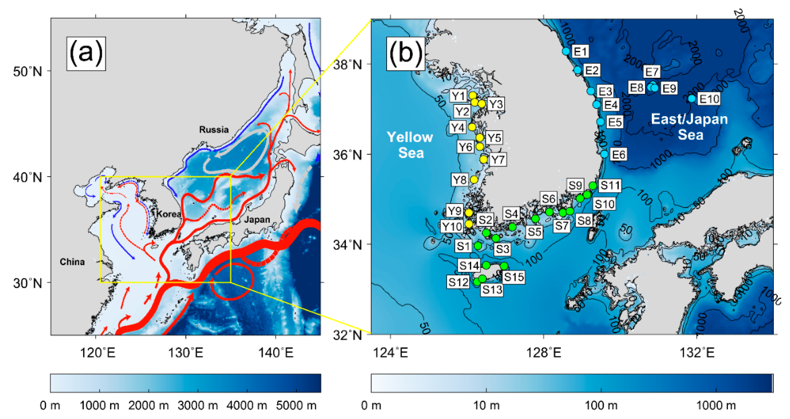
2.2. In-Situ Temperature

Herein, we used temperature data from the KMA coastal wave buoys to validate SST analyses in the coastal region around the Korean Peninsula (Figure 1b) [69]. To improve marine weather monitoring, the KMA has been operating 66 coastal wave buoys, as shown in Figure 1b. Although the main purpose of these coastal wave buoys is to record ocean wave information, 30-cm depth water temperatures are also measured at several stations in the coastal region off the Korean Peninsula. Temperature measurements from these coastal wave buoys are excluded from the GTS network and diverse SST composite products in the global ocean. Thus, temperature data from these wave buoys can be essential independent data that is applicable for validating the accuracy of each SST database.
During the study period, water temperatures were measured at 35 coastal wave buoys located around the Korean Peninsula (Table 2), with 10 of these located in the EJS, 15 buoys in the southern region, and 10 buoys in the Yellow Sea, as shown in Figure 1b. The precision and temporal resolution of their water temperature measurements were 0.1 K and 1 hour, respectively. The coastal wave buoys were located in the shallow regions over depths ranging from 16.5–51.0 m and at distances from the coast ranging from 0.14–13.36 km. Their water temperature data for the period of 2014–2018 were quality-controlled according to the appropriate quality control procedure [70], which led to about 5.8% of the data being removed, on the basis that it was probably erroneous.

2.3. Error Analysis Methodology

To compare the SST analysis databases with in-situ temperatures, matchup databases between the SST and in-situ temperatures were produced by considering the nearest positions. In comparison with in-situ measurements, a series of matchup processes was performed while maintaining the resolution of each SST analysis. Due to a change of grid sizes of the CMC product, as described in Section 2.1.2, the nearest grid point of 0.1° grid into 0.2° grid was selected before the matchup procedure. First, the matchup data between buoy temperatures and satellite SSTs were produced and then an average over different time periods (daytime, nighttime, 24-hour averages) were taken, by considering the SST types such as a foundation SST or bulk SST.
Since the buoy temperatures were taken hourly, in-situ measurements were converted to daily-averaged temperatures to have the same temporal interval of temperatures with that of the SST analysis database. To investigate the effect of diurnal variation of in-situ temperature, daily-averaged temperatures using daytime only, nighttime only, and all data were calculated.
To quantify the accuracy of the SST analyses, statistical parameters, such as bias, RMSE, and combined error (Ecom), which was suggested as a concept of error radius, considering the importance of RMSE and bias to be identical [71], were used with these being, respectively, defined as follows:
B i a s = 1 N i = 1 N ( x i y i ) ,
R M S E = 1 N i = 1 N ( x i y i ) 2 ,
E c o m = R M S E 2 + B i a s 2 ,
where x i represents the SST analysis, y i stands for the buoy temperature, and x ¯ and y ¯ represent the average values of the SST analysis and buoy temperature, respectively. N represents the number of the data [70].
For inter-comparison between SST analyses, these datasets with different resolutions need to be re-gridded to an identical grid [42,43,45]. Therefore, all SST products were re-gridded into 0.25° grids, using the nearest neighborhood method, by keeping the original values, to use comparable grids in the SST database inter-comparisons.

3. Results

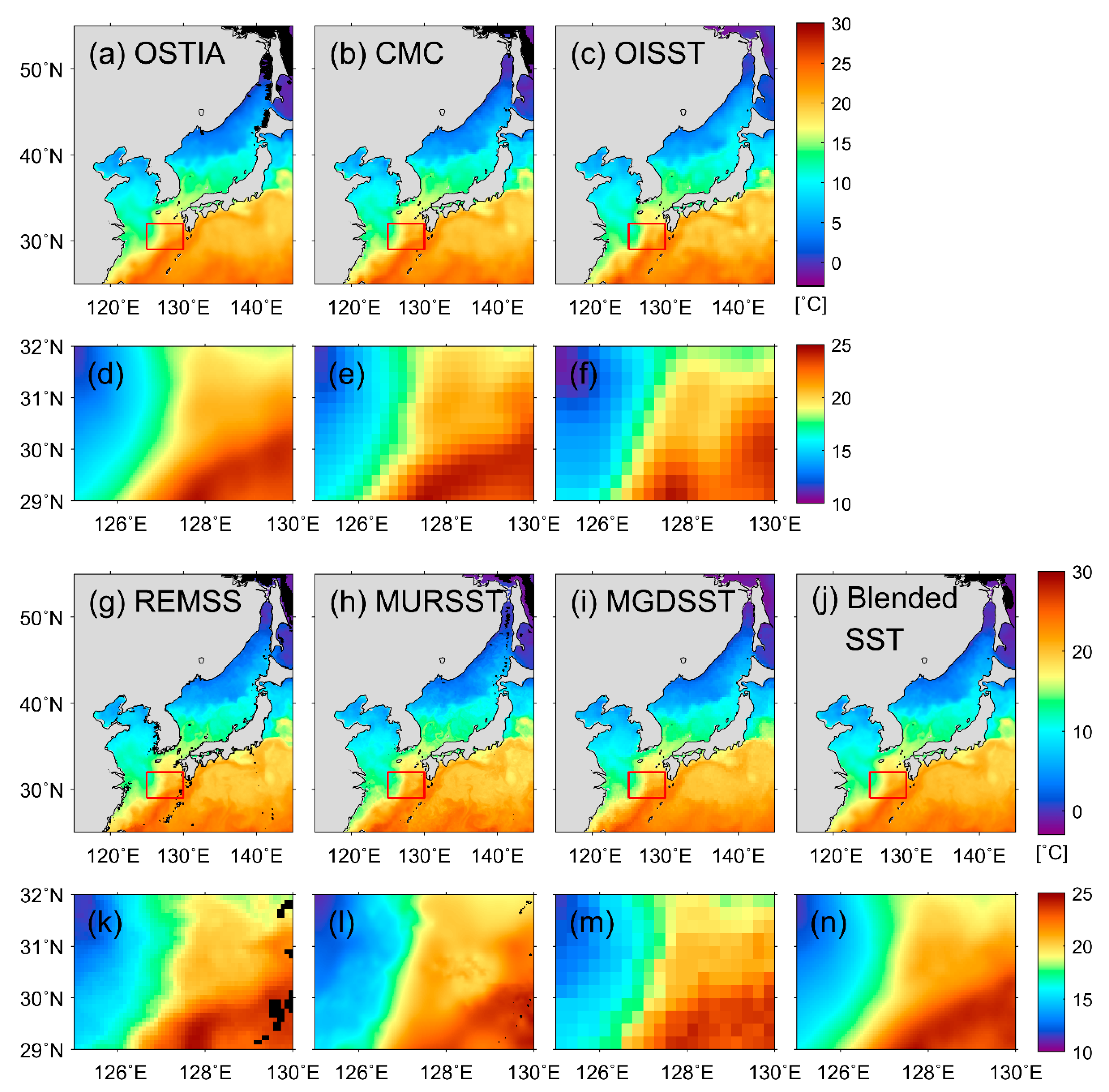
3.1. Spatial Distribution of SST analyses

Figure 2 shows the examples of the spatial distribution of SST analysis data in the marginal seas of the Northwest Pacific on 15 April 2016. Overall, the SSTs of the seven databases showed a similar meandering path of the Kuroshio Current in the Northwest Pacific and spatial distributions of the subpolar front along 40°N in the EJS, as indicated in Figure 2a–c,g–j [51,72]. On the contrary, the enlarged portions of the region around the Kuroshio Current, as shown in Figure 2d–f,k–n, revealed relatively small-scale features, depending on the grid resolutions of the SST databases. As shown in Figure 2h,l, when compared to other SST analyses, the MURSST with its 1-km spatial resolution presented not only large-scale structures of the oceanic phenomena but also small-scale features. The SST analysis of REMSS, with its 9 km spatial resolution, also detected relatively small-scale features (Figure 2g,k).
By contrast, most SST analysis databases such as the CMC analysis, OISST, and MGDSST—with their relatively low spatial resolutions of more than 0.2°—failed to show distinctive small-scale features (Figure 2e,f,m). It was conspicuous in the enlarged plots that the OSTIA (Figure 2d) and the Blended SST database (Figure 2n) expressed large-scale features without small-scale noises [4].

3.2. Comparison between SST Analysis Data and In-Situ Measurements

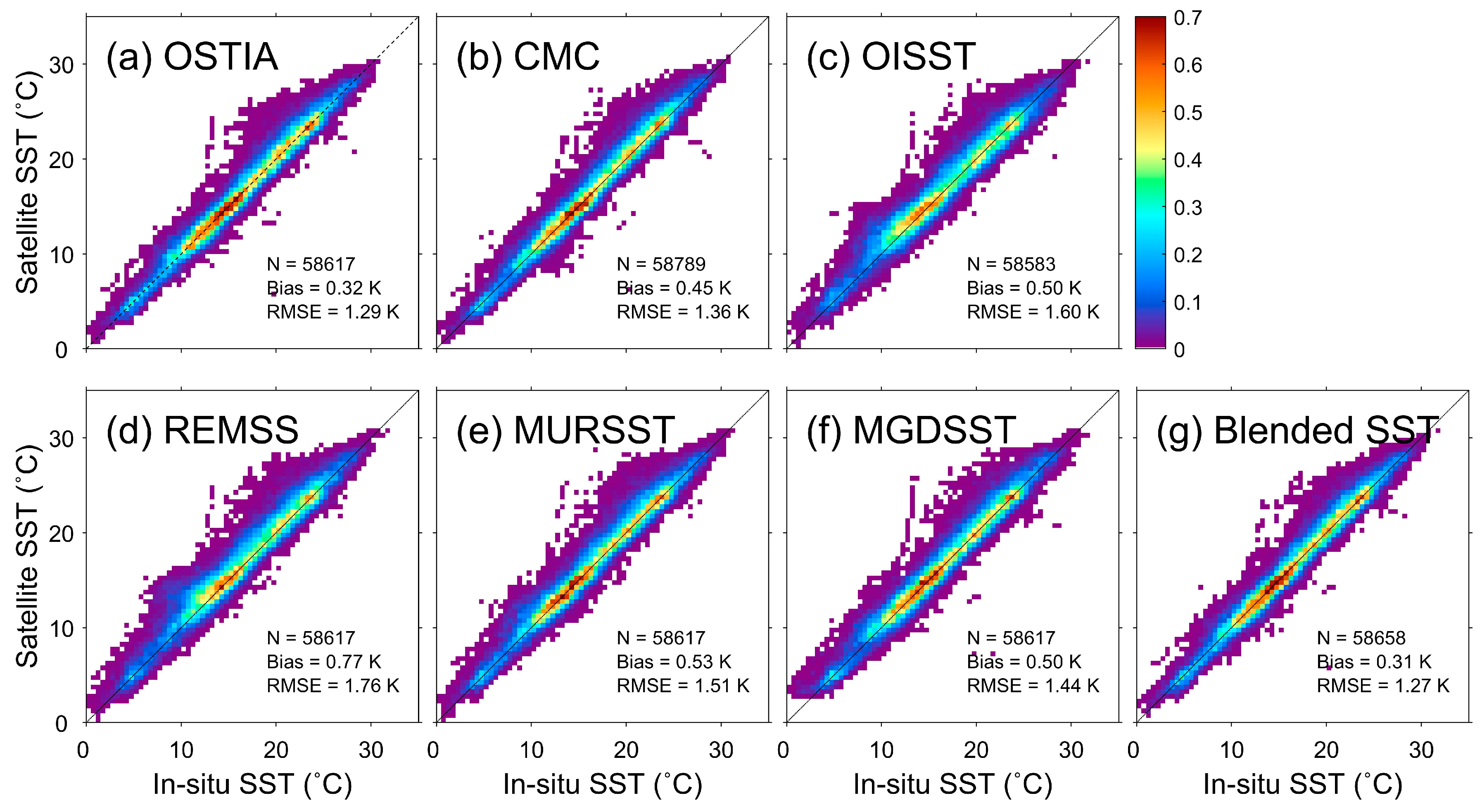
3.2.1. Accuracy Assessments of SST Databases

To determine the accuracy of SST analysis data in coastal regions, in-situ temperatures from the coastal wave buoy of the KMA were compared with each database (Table 3). The SST analyses showed positive bias errors of 0.26 K or more and RMSEs from 1.26 to 1.72 K in the daytime (from 6 am to 6 pm KST), 1.29 to 1.76 K in the nighttime (from 6 pm to 6 am KST), and 1.27 to 1.74 K for daily-averaged temperatures, using the hourly temperature measurements. All products showed distinct positive biases, which were about 0.06 K higher during the night than during the day. This implied that in-situ temperatures, which were measured at a depth of approximately 30 cm, were slightly affected by diurnal variation. Therefore, in order to produce foundation SSTs using in-situ measurements, daily-average SST should be combined using only the nighttime data. Since OSTIA, REMSS analysis, MURSST, and MGDSST are foundation SSTs with the diurnal variation removed [4,39,63,65], the comparisons were performed for in-situ temperatures averaged over nighttime hours from 6 pm to 6 am. Except for these three products, all validation procedures for the CMS, the OISST, and the Blended SST were established against daily-averaged in-situ temperatures obtained for a day corresponding to the date of the satellite data (Figure 3).
As shown in Figure 3, it is worth noting that all SST analyses exhibited positive biases of 0.31 K or more. The Blended SST database presented the lowest bias of 0.31 K, while the REMSS analysis showed the highest bias of 0.77 K, revealing considerable differences between the databases (Figure 3d,g).

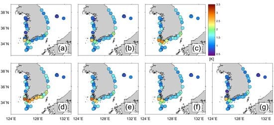
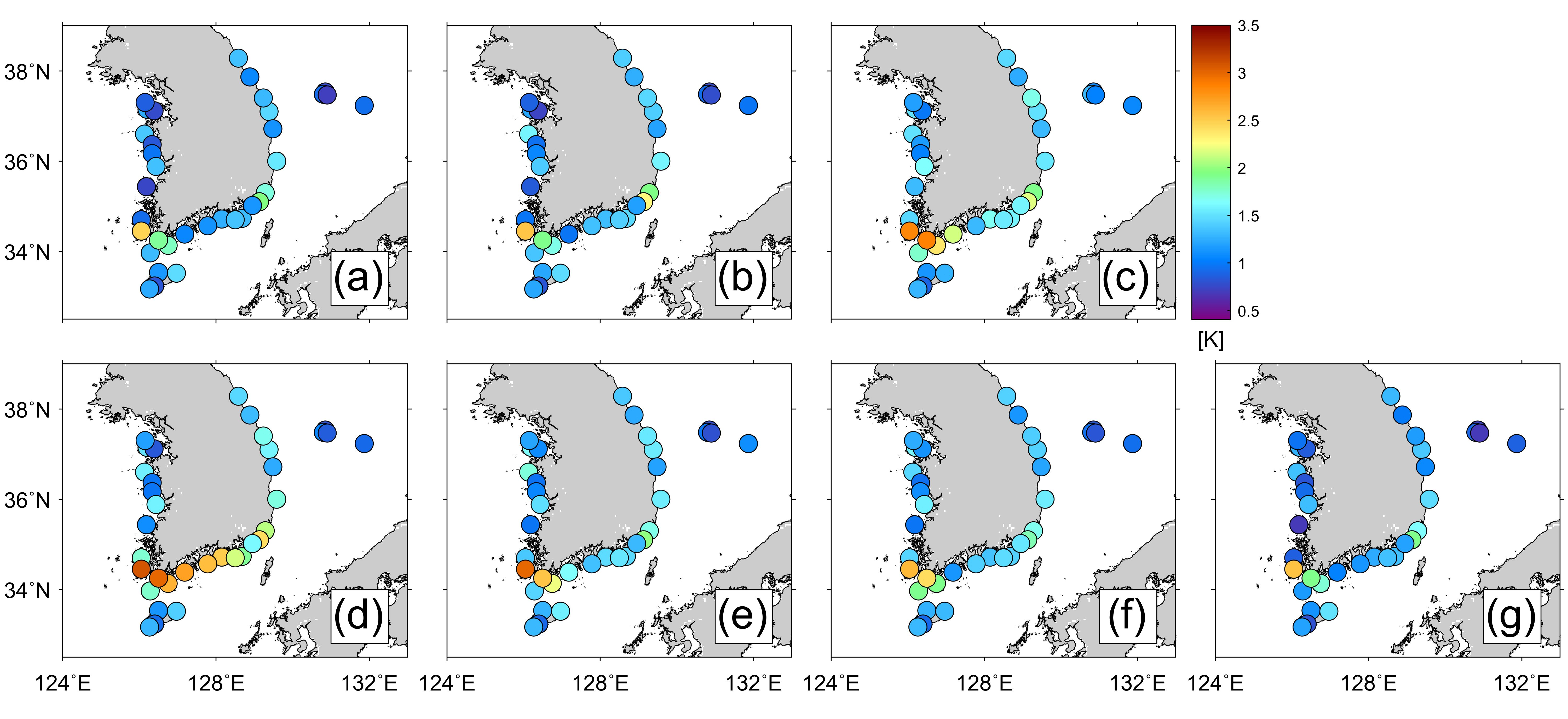
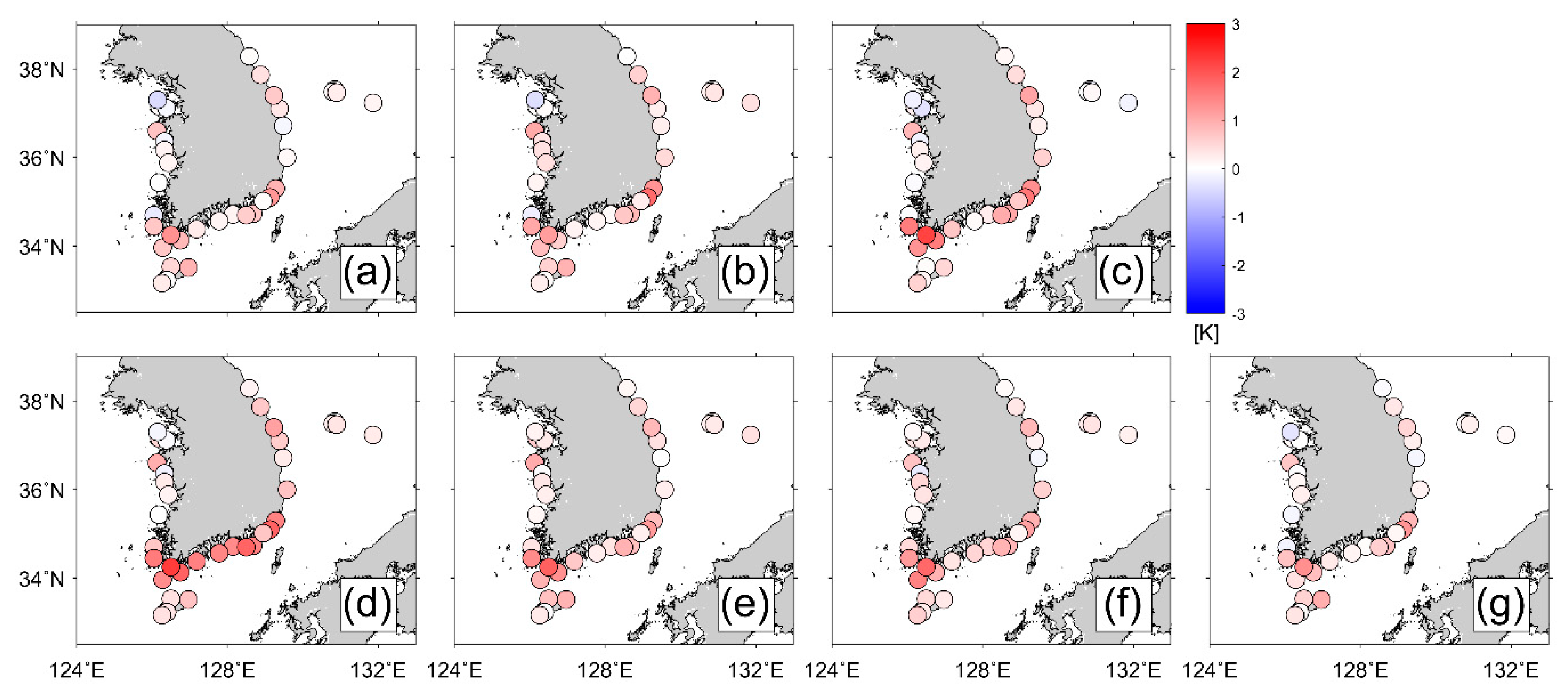
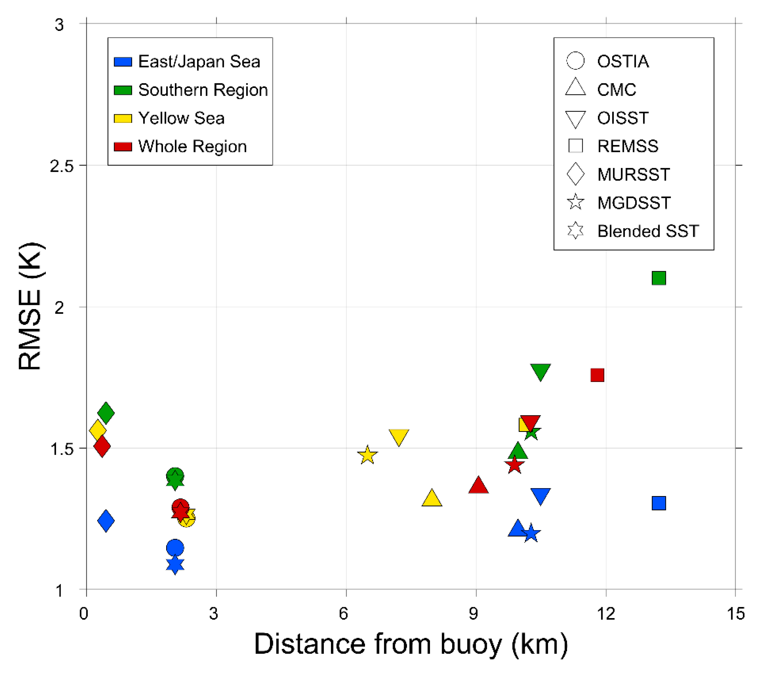
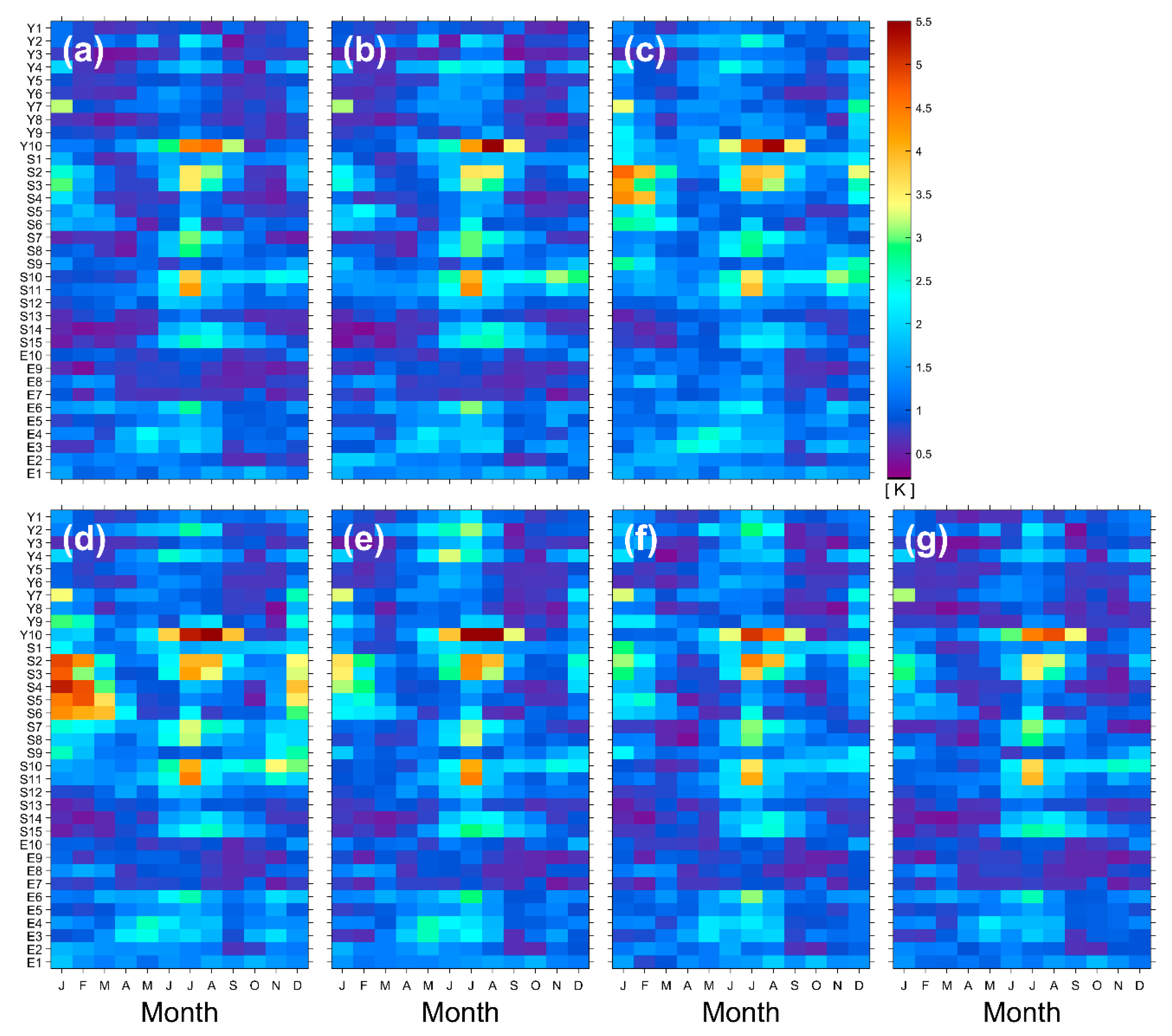
3.2.2. Characteristics of Spatial Distribution of SST Errors

In order to understand the characteristics of the spatial distribution of errors in the coastal region of the Korean Peninsula, the RMSEs and bias errors of SST analysis at each buoy station are shown in Figure 4 and Figure 5, respectively. As shown in Figure 4, the bias error also showed lower amplitudes in the OSTIA and Blended SST database, compared to other products across the entire region, whereas the REMSS analysis showed a distinct positive bias (0.31–2.27 K) in the southern region. Comparisons of SST data with in-situ temperatures yielded bias errors from –0.41 (Y1) to 1.30 K (S2) for the OSTIA data, –0.38 (Y1) to 1.74 K (S10) for the CMC data, –0.33 (Y3) to 2.20 K (S2) for the OISST data, –0.14 (Y5) to 2.27 K (S2) for the REMSS data, –0.02 (Y5) to 1.87 K (S2) for the MURSST data, –0.24 (Y5) to 1.78 K (S2) for the MGDSST data, and –0.31 (Y1) to 1.34 K (S2) for the Blended SST data, as shown in Figure 4.
Consistent with the previous results, the OSTIA, CMC analysis, and the Blended analysis had relatively low RMSEs (Figure 5a,b,g), which contrasted with the REMSS analysis with its comparatively higher RMSEs ranging from 0.80 to 3.08 K than other analyses (Figure 5d). The RMSE at each buoy station were relatively small, ranging from 0.69 to 1.71 K in the open ocean of the EJS. These small errors were detected in the offshore region, far from the eastern coast of Korea, while the higher values were found in the southwestern region. In the EJS, RMSEs less than 2 K were produced in both the coastal region and the open ocean. In contrast, the RMSEs of the SST analysis in the southern region and the Yellow Sea had large regional deviations amounting to 2.39 K. In the southern region, the RMSEs were mainly high in the vicinity of buoys S2 and S3, while in the Yellow Sea, the RMSEs were high at buoys Y2 and Y4, and especially at buoy Y10.
Considering the RMSE of OSTIA for the in-situ temperature at each coastal wave buoy station, the minimum RMSE of 0.71 K was shown by buoy E9, whereas the maximum RMSE of 2.46 K was shown by Y10 (Figure 5a). For the CMC analysis, the minimum RMSE was 0.74 K at Y3, whereas the maximum was 2.54 K at Y10 (Figure 5b). The RMSE of OISST ranged from 0.89 (S13) to 2.87 K (S2) (Figure 5c). The minimum and maximum RMSE values of REMSS analysis were 0.80 K (E7) and 3.08 K (Y10), respectively (Figure 5d). The RMSE of MURSST also showed a minimum of 0.79 K (E7) and a maximum of 3.00 K (Y10) (Figure 5e). For MGDSST, the minimum RMSE of 0.82 K was seen at E9, whereas the maximum of 2.60 K was seen at Y10 (Figure 5f). The minimum and maximum RMSE values of the Blended SST analysis were 0.67 K (E9) and 2.54 K (Y10), respectively (Figure 5g).
Since the seas around each side of the Korean Peninsula had very different bathymetry and shorelines, the relative accuracies of the data for the different seas—the EJS, the Yellow Sea, and the southern part of the Korean Peninsula—were evaluated, and the results were displayed in Figure 6, following the RMS-bias map style suggested by Jang et al. [71]. In the EJS, all analyses had low bias errors and RMSEs less than 0.43 K and 1.34 K, respectively, whereas in the southern region, the bias errors and RMSEs were comparatively high ranging from 0.56 to 1.26 K and 1.39 to 2.10 K, respectively. In the Yellow Sea, all analyses had bias errors and the RMSEs ranged from 0.09 to 0.44 K and 1.25 to 1.58 K, respectively. In Figure 6, it could be seen that RMSEs increased as bias errors increased in all regions. The spatial distribution of the RMSE-bias plot of the Yellow Sea was similar to that of other regions, but an offset occurred in the RMSE direction. In the Yellow Sea, RMSE values were higher, although the mean bias values were similar to those in the EJS. This indicated that high RMSE values were due to the high variability of SST errors in the Yellow Sea, which were distinct from the EJS and the Southern region.
When the combined errors (Ecom) were estimated using the method proposed by Jang et al. [71], in the EJS, most of the values were small compared to other regions, whereas in the southern region, they were larger than other regions. Regardless of the regions, the SST tended to be most accurately estimated in the OSTIA and the Blended SST. In the EJS, the MGDSST showed the relatively high accuracy, exhibiting a combined error of about 1.23 K. In the southern region and the Yellow Sea, the CMC analysis showed a higher accuracy than other SST analyses except for the OSTIA and the Blended SST, with combined error values of 1.61 K and 1.35 K, respectively. The combined errors of the REMSS product over the whole regions were quite high—1.37 K for the EJS, 1.63 K for the Yellow Sea, and 2.45 K for the southern region.
Although the validation was performed based on independent data—by excluding the GTS buoy data that was used in generating the SST analysis database—similar temperatures might be used in this study, as there are many coastal wave buoys in quite close proximity to the GTS buoy stations. We therefore assessed the accuracy of the SST database again, by removing the buoys located within 30 km of the corresponding GTS buoys. This led to a tendency in the combined errors to increase by 0.1–0.3 K, while the accuracy ranking of the SST databases showed little change.
Overall feature of the SST errors suggested potential influences from both bathymetry and coastline complexity, especially where there were many small islands, such as along the southern and western coasts of the Korean Peninsula. As the spatial resolution of the various SST analyses varied from 1 to 25 km, it was also conceivable that the SST errors varied in relation to the distance between each buoy and the center of grid of SST analysis corresponding matchup point. Moreover, in the coastal region, the SST analysis errors were likely to be intensified, as the spatial scales of SST variability were relatively smaller, and temporal and spatial variabilities of SSTs were much greater than those in the open ocean [23,26,73]. Figure 7 indicates the SST analysis errors, plotted with respect to region, as a function of the distance between position of coastal buoys and center of grid of SST analysis data. Here it can be seen that, although the spatial resolution REMSS was about 9 km, the distance from the buoy was more than 10 km because SST was not estimated in the sea near the coast. The distances for the CMC, OISST, and MGDSST with resolutions of 20 km or more from the buoy stations showed ranges of 10–15 km. Overall, as the distance between the SST analysis and their respective buoys increased, the RMSE also tended to increase. This tendency was evident in the southern regions and the Yellow Sea, but not in the EJS, as shown with the blue symbols, regardless of the source of the SST database.

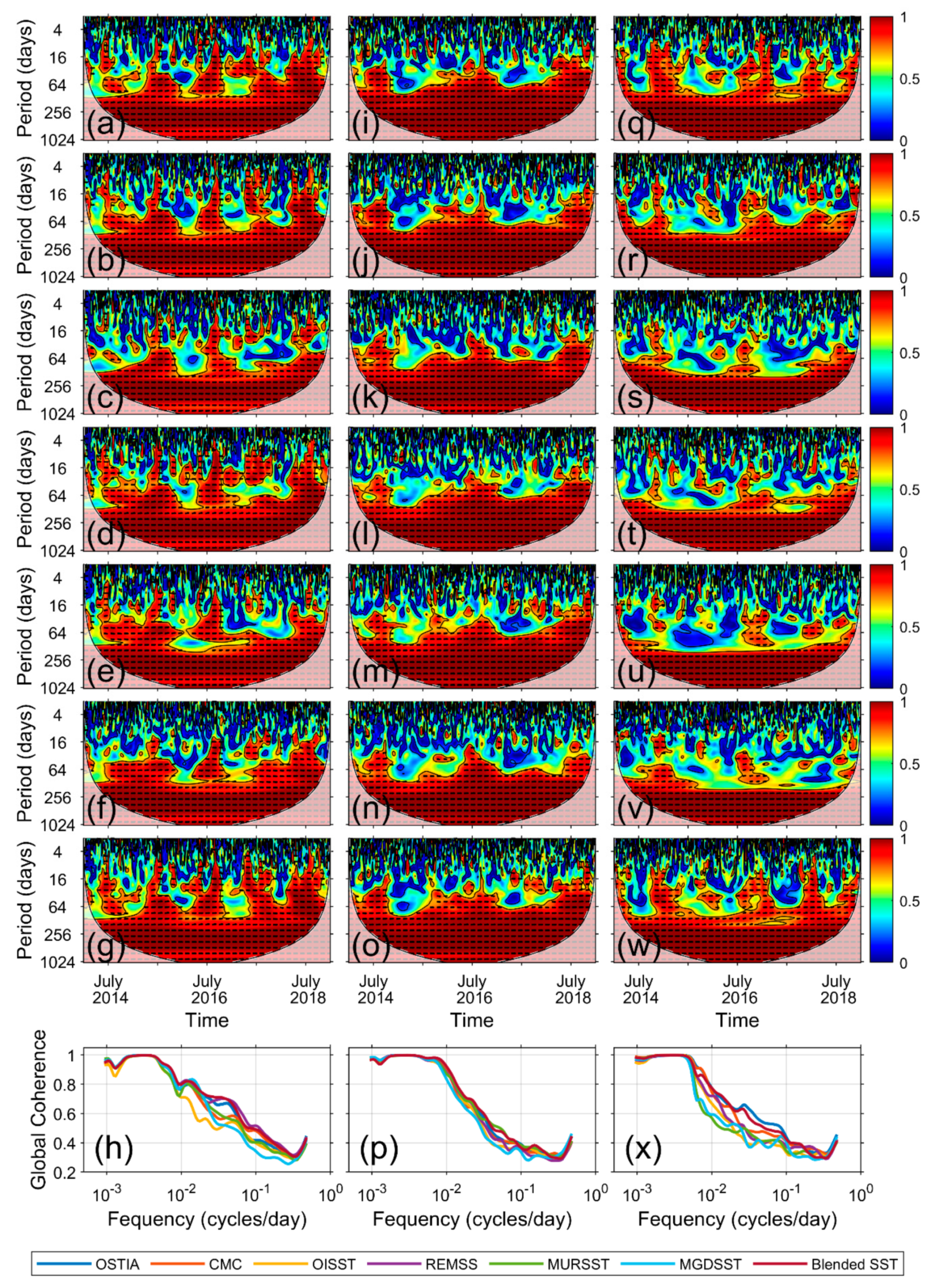
3.2.3. Comparison of Wavelet Coherence

In addition to the spatial distributions of the SST errors, it was also considered important to review the temporal characteristics of the SST analysis data errors, to fully understand the properties of SST products—and this was done by comparing them with in-situ temperatures (Figure 8). In order to compare temporal variability in the differences between the SST analyses and in-situ temperatures, the wavelet coherence between them was calculated at three representative marine stations (E4, S2, and Y10). These stations were selected as they had relatively large RMSEs and were located on each side of the study area (Figure 8).
Wavelet coherence between OSTIA SST and in-situ temperatures at the E4 station of the EJS was seen to have a relatively high coherence of greater than 0.8 at longer periods of over 64 days, during the entire study period, as well as over much shorter periods centered at 16 days, especially in summer (Figure 8a). This pattern was found to be repeated by other products, except for the OISST and MGDSST product, which showed no overall seasonal variation in coherence with only nominal values even in summer, at periods of less than 64 days (Figure 8c,f). As shown in the averaged coherence values with respect to the period in Figure 8h, all SST products kept their coherence high (>0.8) at longer periods of more than 180 days. This high coherence of over 0.8 for long periods (>180 days) indicated that both in-situ measurements and SST analyses dominantly reflected the annual variations of SST at a range of more than 10 K in the coastal regions around the Korean Peninsula. For shorter periods (<64 days), however, the coherences tended to gradually decrease to about 0.3 without statistical significance. At this high-frequency range from 64 days to 4 days, the REMSS data produced relatively high coherence, while the MGDSST resulted in the lowest similarity with in-situ SSTs (Figure 8h).
For the station S2, in the southern coast region, the coherence diagrams of all SST products were quite similar (Figure 8i–o). This similarity was confirmed by the low level of scattering of the differences between the products with a narrow range of coherence values, as shown in Figure 8p. In contrast to this, relatively high temporal coherence variability was seen for Y10 in the Yellow Sea, where the OSTIA and the Blended SST had a relatively high coherence of greater than 0.8, in comparison to other SST analyses products by occupying extensive areas in the coherence diagram (Figure 8q–w). The detailed variability of coherence was different at the three buoy stations, but overall, it was high over the long-term period of >180 days and low over the short-term period of <64 days. This demonstrated that SST analyses simulated long-term fluctuations, such as annual variation, similar to in-situ measurements but did not properly simulate short-term period fluctuations.

3.3. Inter-Comparison of the SST Products

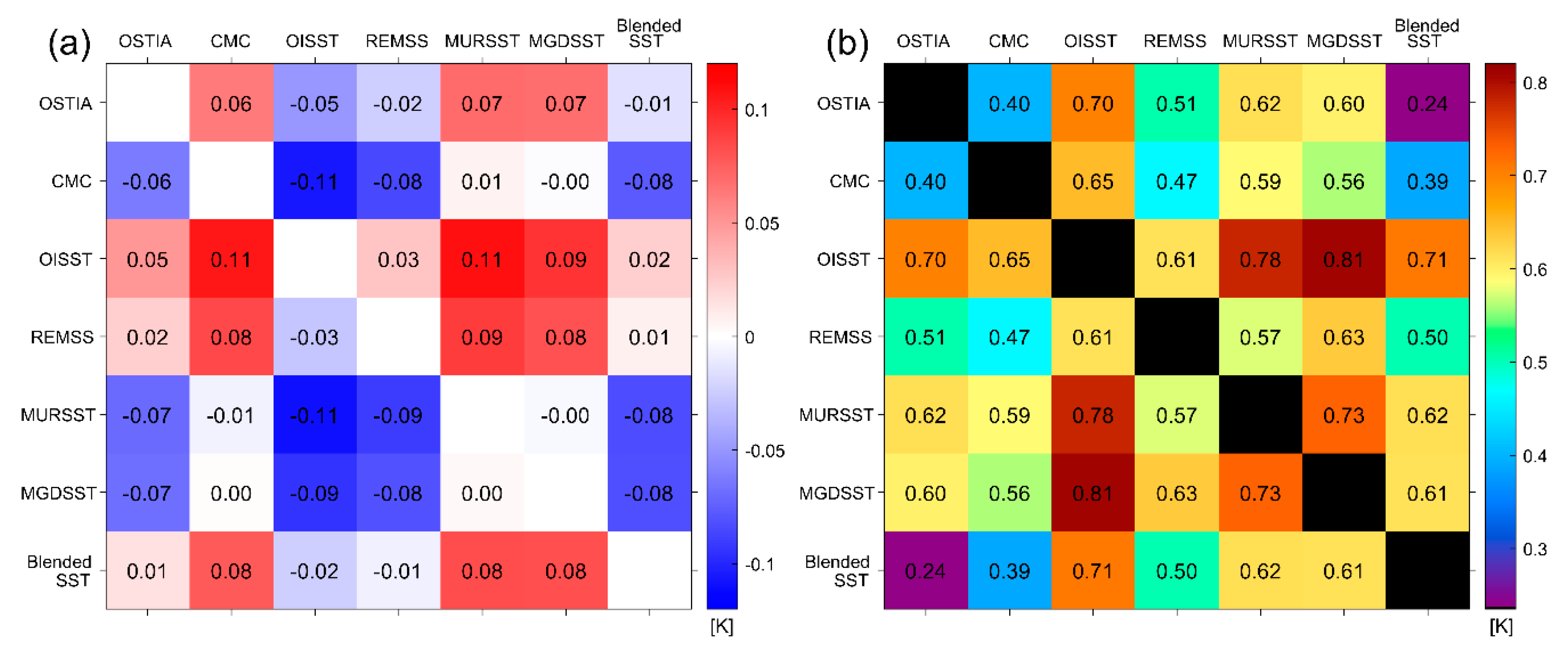
3.3.1. Errors of Differences between the SST Products

For inter-comparison between the SST products, spatial averaged RMS difference and bias between each SST analysis were estimated for the entire marginal sea region of the Northwest Pacific (25–55°N, 115–145°E), as shown in Figure 9. The bias and RMS errors in each grid in Figure 9 were estimated using temperature differences between each SST product listed at the top of the plot and the other SST product indicated on the left side (column minus row). For example, the error of −0.08 K in the 4th column and the 2nd row in Figure 9a indicated the bias error of REMSS SST minus CMC SST. In contrast to normal RMSE and bias errors, these errors between the SST products did not indicate the degree of each SST product’s accuracy, but rather identified the level of similarity between the arbitrary dataset pairings with no involvement of in-situ temperatures.
The SST differences (OSTIA SST minus other SST analysis), along the first column of Figure 9a, had biases ranging from −0.07 to 0.05 K for the other analyses. The CMC analysis differences from other products, as indicated in the second column, showed positive biases in the range of −0.01 to 0.11 K, while the OISST differences showed negative biases from −0.11 to −0.02 K. The REMSS and Blended SST also showed negative biases for almost all analyses, with the exception of the OISST. The MURSST and MGDSST showed positive biases of more than 0.07 K in the case of the differences from OSTIA, OISST, REMSS analysis, and Blended SST data in the Northwest Pacific Ocean. The MURSST, MGDSST, and OISST were consistently biased high or low, relative to the other products.
As can be seen in Figure 9b, the most similar SST variability with the lowest RMS differences of about 0.24 K was found between the OSTIA and Blended SST data products, while the lowest similarity of SST variability with the highest RMS difference of 0.81 K was detected between the OISST and the MGDSST products. When the other analyses were used as reference SSTs, the CMC analysis showed the smallest RMS difference value and the OISST showed the largest, overall, as shown in the 2nd and 3rd columns, respectively (Figure 9b). For the other SST analyses, the OSTIA product showed RMS differences ranging from 0.24 K with the Blended SST analysis to 0.70 K with the OISST data. The CMC analysis also showed the smallest RMS difference (0.40 K) with the OSTIA SST data and the largest RMS difference (0.65 K) with the OISST data. The RMS difference of the OISST presented a minimum value of 0.61 K for the REMSS analysis and a maximum value of 0.81 K for the MGDSST data. The REMSS analysis showed the lowest difference for CMC analysis (0.47 K) and the most prominent difference for the MGDSST (0.63 K). The maximum and minimum RMS differences for the MURSST were 0.57 K (REMSS analysis) and 0.78 K (OISST), respectively, and those for the MGDSST data were 0.56 K (CMC analysis) and 0.81 K (OISST), respectively. Blended SST presented the smallest RMS difference for OSTIA (0.24 K) and the largest RMS difference for OISST (0.71 K).

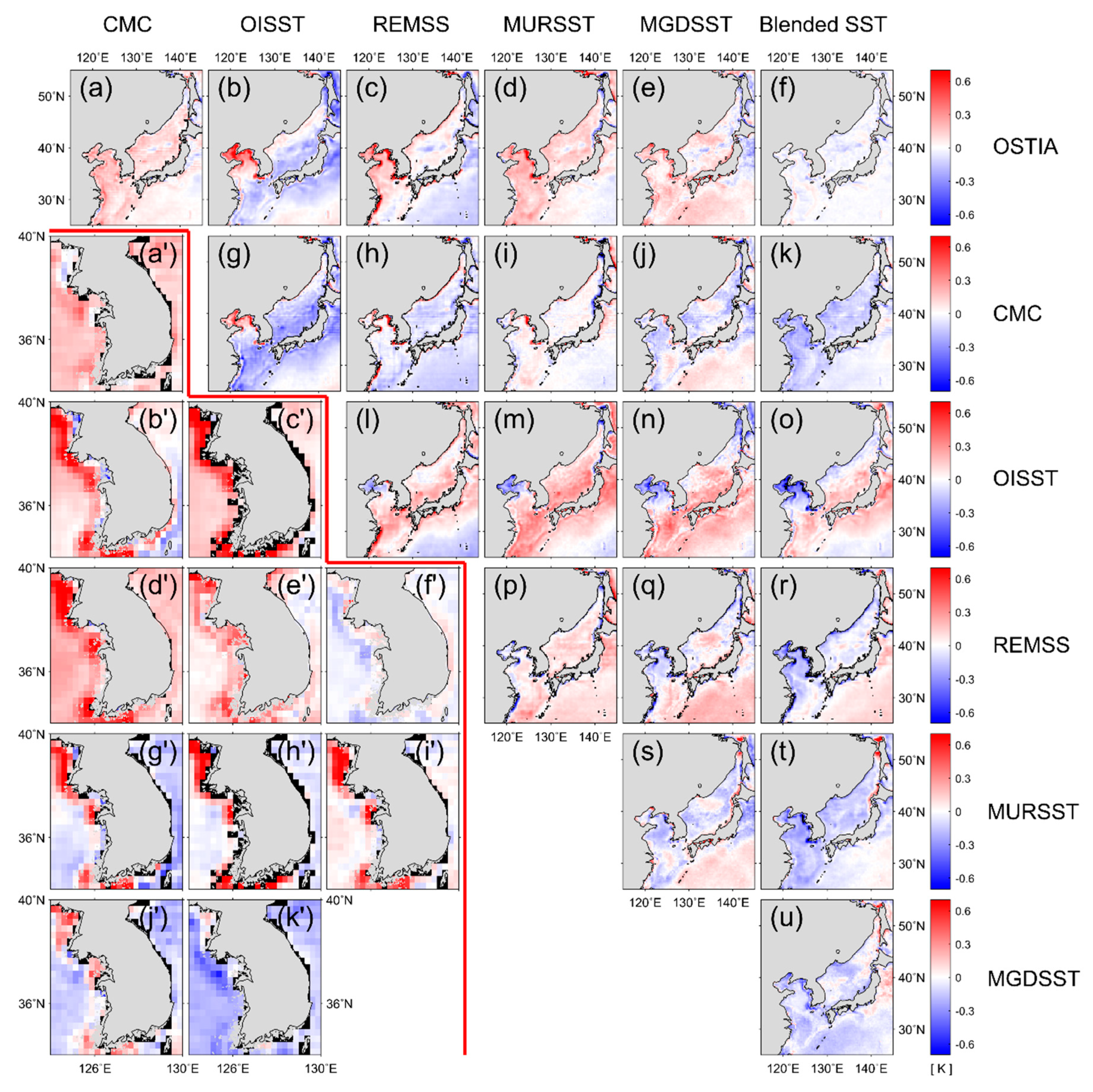
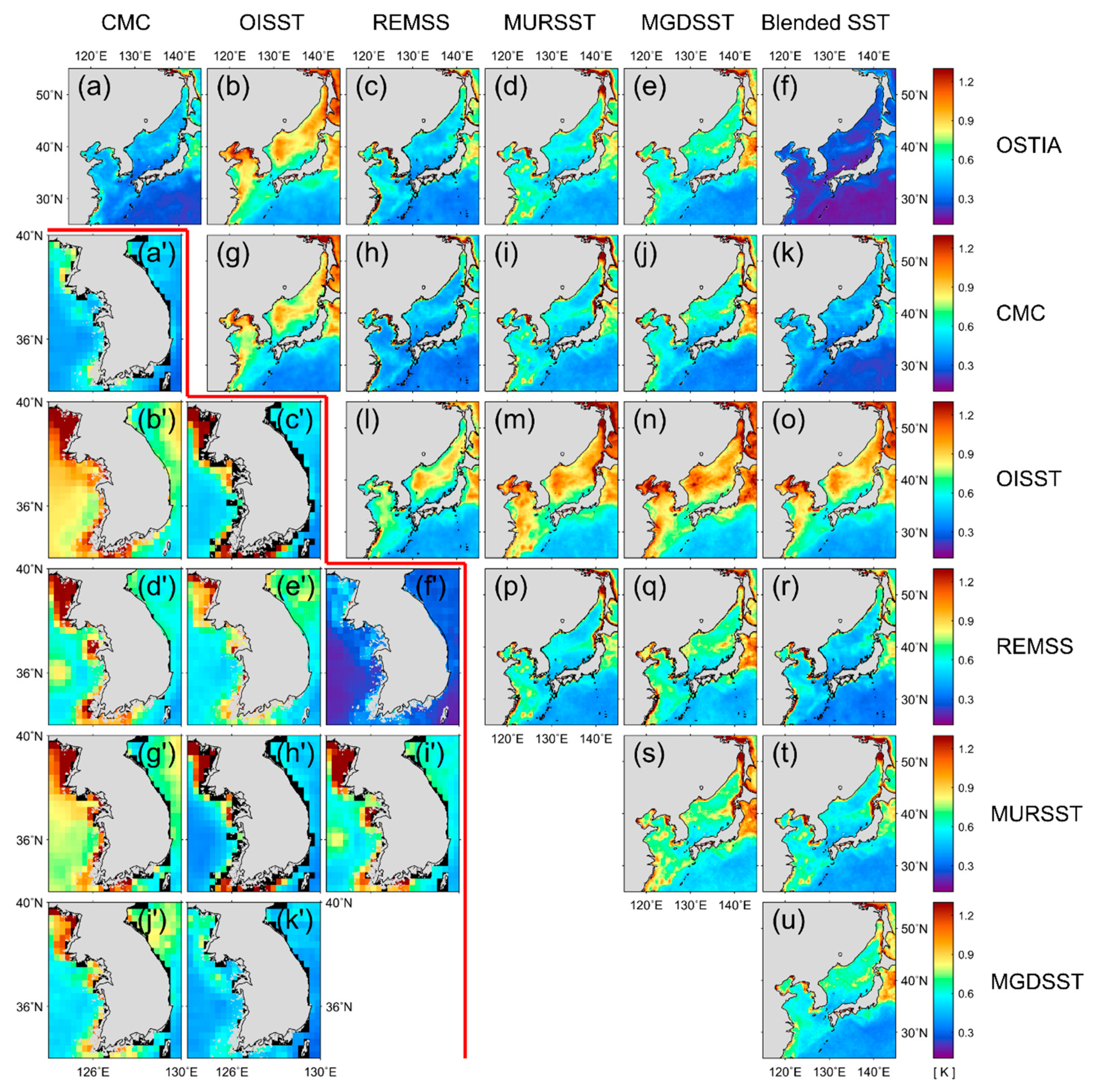
3.3.2. Spatial Distribution of Variability between the SST Products

The spatial distribution of the bias that occurred between the SST analyses are depicted in Figure 10. CMC, MURSST, and MGDSST SSTs showed positive bias in most regions, when compared to the OSTIA SSTs (Figure 10a,d,e). The OISST against OSTIA SST comparison, OISST minus OSTIA SST, had positive biases in the western coastal region of Korea and in the northern region of the Yellow Sea, however, most other regions—the southern regions of EJS, the East China Sea (ECS), and the eastern coastal region of Japan, indicated negative biases (Figure 10b). The REMSS analysis also showed a weak negative bias of −0.2 to −0.1 K in the Northwest Pacific, and a positive bias in the Yellow Sea (<0.6 K), as shown in Figure 10c. The Blended SST against OSTIA showed near-zero biases in most regions of the Northwest Pacific (Figure 10f).
When CMC data were used as a reference (the 2nd row of Figure 10), most SST analyses showed distinctively negative biases, with the exception of some coastal regions around the Korean Peninsula that showed positive biases (Figure 10g–k).The biases of the REMSS analysis, MURSST, MGDSST, and the Blended SST for the OISST presented similar distributions with positive values in the southern region of EJS, the ECS, and the eastern coastal region of Japan, and negative values in the western coastal region of Korea and the northern region of the Yellow Sea (Figure 10l–o). The MURSST, MGDSST, and the Blended SST had weak positive biases in the open ocean of the Northwest Pacific, compared to the REMSS analysis (Figure 10p–r). On the other hand, in the Yellow Sea, MURSST showed positive bias, and MGDSST and the Blended SST showed negative biases. In the EJS, the MURSST and the Blended SST showed positive and negative biases, respectively. As shown in Figure 10s, the bias of MGDSST for the MURSST as a reference was weakly negative in the EJS and the Yellow Sea, and weakly positive in the Northwest Pacific. Blended SST for both MURSST and MGDSST had negative biases in most regions of the Northwest Pacific (Figure 10t,u).
The Investigation into the coastal regions found that high amplitude of biases applied along the western part of the Korean Peninsula, as illustrated by most of the plots in Figure 10. The prime symbols in Figure 10 represent enlargements of the unprimed symbols in each plot from (a) to (k)—for instance, (a’) is from (a) in Figure 10. The enlargements of these coastal regions revealed a peculiar bias (>0.4 K), as shown in the comparisons of OSTIA and CMC SSTs, with other products of the OISST, the REMSS, the MURSST, the MGDSST, and the Blended SST, along the southwest and south coasts of the peninsula (Figure 10a’–k’). These features were more pronounced in comparison with CMC analysis.
Figure 11 shows the spatial distribution of RMS difference between SST analyses for each grid in the Northwest Pacific for the period of 2014–2018. When using the OSTIA SSTs as a reference, as shown in the first row of Figure 11, the Blended SST analysis showed the small RMS difference with the OSTIA SSTs in most of the marginal seas (<0.3 K), especially the smallest RMS difference in the Kuroshio region of the Northwest Pacific below 0.2 K (Figure 11f). On the contrary, the OISST showed relatively high RMS difference amounting to 1.2 K in the northern region of the EJS (>0.8 K), in the Bohai Sea, and along the western coastal region of the Yellow Sea (~1.2 K), as seen in Figure 11b. This result was consistent with relatively high RMS difference values of OISST, as exhibited in the 3rd column of Figure 9b. The SSTs for REMSS, MURSST, and MGDSST (Figure 11c–e) presented relatively higher RMS difference in comparison with OSTIA SSTs, after the CMC analysis (Figure 11a), although this RMS difference was lower than OISST, as seen in Figure 11b. It is noted that the REMSS with the highest variability at the southwestern coast yielded relatively small variability in the offshore regions of the Northwest Pacific, as shown in Figure 11c,h,l,p–r. Comparison between Figure 11b and Figure 11g illustrates that the variability of the OISST was similar to that of the OSTIA for the CMC analysis. In addition, the variability for the REMSS analysis, MURSST, and MGDSST (Figure 11h–j), which were calculated using CMC analysis as the reference, were also similar to those calculated by reference to OSTIA (Figure 11c–e). However, the variability of the Blended SST with CMC analysis as a reference (Figure 11k) was amplified than that with OSTIA as a reference (Figure 11f).
The RMS difference for the REMSS analysis, MURSST, MGDSST, and the Blended SST, estimated using OISST as reference, were greater than 1.0 K in the EJS and the Yellow Sea (Figure 11l–o). This implied that the OISST embodied a larger variability from the other SST analyses. RMS difference of the MURSST, the MGDSST, and the Blended SST against the REMSS analysis (Figure 11p–r), the MGDSST and the Blended SST against the MURSST analysis (Figure 11s,t), and the Blended SST against the MGDSST (Figure 11u) were relatively moderate in comparison to the OISST case.
Most of the results showed high variability in the coastal regions and low variability off-shore. The coastal region enlargements (Figure 11a’–k’) demonstrated remarkably high RMS difference, exceeding 1.2 K, especially in the southwestern coastal region of the Korean Peninsula. This implied that most SST products tended to be amplified with the viewpoint of variability, especially at specific coastal locations off the western coast of the Korean Peninsula. As illustrated in Figure 11d’,i’, higher variability of the SST database (>1.2 K) became quite evident at specific coastal regions, such as the southwestern corner, the western corner of the central area, and the North Korean coastal region. These regions are also associated with tidal mixing zones from strong tidal currents and shallow bathymetry, or with frequent sea fog [74,75]. More details about tidal current-related influences on SST differences are dealt with in the final part of Discussion.

4. Discussion

4.1. Absence of Microwave SST at Coastal Region

Comparative studies between global SST analysis products and in-situ SST databases in the coastal regions are relatively insufficient, even when considering that some studies have shown amplification of SST errors at high-latitude sea-ice transition zones and coasts [42]. In global oceans, the accuracies of the SST analysis have been reported to be within 1 K, through long-term validation of the SST analysis, using comparison with in-situ measurements and inter-comparison [40,41,42,43,44,45]. It has been reported that such differences between daily SST analyses and the daily SSTs from buoys can be caused by several factors, including differences in thermometer types, observation depths, or the specific schemes for estimation of the daily SST [24,42]. As well as these factors, the verification results obtained also revealed noticeable deviations with high RMSEs, amounting to 2 K, for the coastal regions along the Korean Peninsula.
Except for the OISST data, all SST analyses used herein included microwave SSTs as input data [4,31,35,36,39,66]. Microwave SSTs cannot be used within 50 km of the coast due to land contamination, and exhibit a bias for up to 150 km seawards from the coast [28,29]. Figure 12a shows an example of the results achieved in the absence of AMSR SST observations in the coastal regions around the Korean Peninsula on 25 April 2016. Even the probability of AMSR observations at each point using all 2016 data, showed zero probability for the coastal areas (Figure 12b), indicating that it is important to have either IR SSTs or in-situ temperature measurements to produce SST analyses. However, it is difficult to obtain IR-based SSTs in the presence of clouds or sea fog and in coastal regions (e.g., [76,77,78]). In such situations, SST analysis data in the coastal region can be affected by microwave SSTs far from the coastline, within a space decorrelation scale in the optimum interpolation procedure [4,75]. Under severe cloud conditions, pixels near the shore tend to be alternatively replaced by background SST values or by climatology SSTs.

4.2. Effect of Tidal Mixing and Upwelling

As shown in Figure 13, monthly variation of RMSEs of SST analyses for the in-situ measurements in each coastal buoy presented prominent seasonal characteristics. The most remarkable feature was the amplification of RMSEs (>3 K) of all SST analyses in the summer (July–August), at the Y10, S2, and S3 buoy stations, which were located in the southwestern coastal region of the Korean peninsula. In the western coastal regions of the Korean Peninsula in the Yellow Sea, there are high tides and strong tidal currents amounting to 5 m s−1 in the shallow waters [53,79]. SST gradients for the tidal front regions in the Yellow Sea and the southwestern region were relatively high at about 0.25 K km−1, due to strong tidal currents and mixing, especially in summer [53,54,74,75]. In summer, SSTs increased to about 28 °C in the offshore region, while in contrast to this, SSTs were greatly reduced to about 10 °C in the onshore regions that were clearly separated from the offshore SSTs, due to strong tidal mixing and fronts with a small tidal front index (log10(H/Umax3), H is the water depth, and Umax is the maximum velocity) of less than 2 [74].
Another monthly variation feature was the increase of the RMSEs of SST analyses in summer at the buoys located in the EJS (e.g., E6 buoy), although the amplitudes were smaller than those in the Yellow Sea (Figure 13). Cold water upwelling often occurs at particular east coast regions of the Korean Peninsula during summer, and this is related to the Ekman transport to the offshore region rather than tidal mixing [80,81]. Similarly, cooler upwelled water increased the IR observation rates, eventually leading to SST bias toward warming. Even though the SST was observed, it showed a negative bias compared to the surrounding region. Therefore, these data were likely to be rejected, as it would be identified as representing either cloud-contaminated pixels or abnormal values, during the quality control procedure. Thus, study was needed to develop a quality control procedure for such extreme events.

4.3. Effect of Front

As shown in Figure 14a, frontal mixing makes surface water cold and produces unclear atmospheric condition with fog or clouds, providing poor conditions for SST estimation [75,82,83]. Such conditions increase the possibility of the use of higher microwave SSTs instead of IR SSTs in the OI procedure for each SST analysis product. This would give rise to positive bias errors in the tidal frontal region in summer, as shown earlier. Figure 14b–g show the relationships between SST gradient, as a measure of SST front magnitude, and the RMS differences of the SST differences between OSTIA with relatively smaller RMS and other SST products (CMC analysis, OISST, REMSS analysis, MURSST, MGDSST, and Blended SST) in the Northwest Pacific of Figure 14a. All plots showed that the larger the SST gradient, the greater the SST product error, as shown in Figure 14b–g. This phenomenon might be encouraged by the differences in the spatial grid size of each SST product and from spatial resolutions of the SST images in the frontal regions.

4.4. Small Spatial Scale of Coastal Oceanic Features

When manifested in the coastal region, ocean-scale phenomena are not only small in spatial scale and structure but are also short in temporal persistence. Therefore, it might be hard for satellite-observed SST data with their spatial resolutions of several kilometers to capture such events [24,84]. Several efforts have been made to implement high-resolution SST databases using VIIRS SST data with its resolution of 750 m as input data [56,63,85], however, it is still necessary to include more high-resolution SST data in both time and space to describe SST phenomena of the coast. To improve the spatial resolution of SST analyses, high-resolution satellite data such as the Landsat-8 SST [86,87] can be utilized in the coastal regions.
In addition, efforts are needed to improve the quality and spatio-temporal resolution of satellite SST in the coastal region [87,88,89]. This is very important for understanding the physical dynamics of the mesoscale and sub-mesoscale SST features that dominate the coastal regions. Additionally, to contribute to improving SST temporal variation of SST analysis, it is necessary to obtain additional in-situ temperature data observed from buoys that are proliferated in the coastal region. Considering that satellite SST observation is difficult, it is suggested that the capacity to observe SST data using more buoy observations needs to be strengthened in coastal regions.

5. Summary and Conclusions

It is essential to identify the advantages and disadvantages of each SST analysis to select the SST analysis optimized for application to the seas around the Korean Peninsula. In this regard, we evaluated the accuracy of, and performed inter-comparison between, seven L4 global, gap-free, gridded, and daily SST products available for the seas around the Korean Peninsula, for the period of 2014–2018.
To investigate how well the global SST databases expressed coastal SSTs along the Korean Peninsula and how applicable they would be for diverse purposes in coastal regions, the accuracy assessment procedure of the SST analyses was performed by comparing their data with in-situ temperatures observed by 35 coastal wave buoys. Our results indicated that SST analyses had a positive bias errors ranging from 0.31 K to 0.77 K and RMSEs ranging from 1.27 K to 1.76 K, in the coastal region of the Korean Peninsula. In all SST analyses, SST errors for in-situ measurements showed similar spatial distributions, except in the dynamic regions with strong tidal currents. Coastal environmental characteristics, including tidal currents and bathymetry, resulted in higher SST errors being detected for the western coast of Korean Peninsula than for the eastern coast.
In addition to the contribution of spatial differences to the SST data errors, temporal scales and similarity between the in-situ temperatures and satellite-based SST database were examined using comparison of the wavelet coherence. This coherence was high (>0.8) for long periods (>180 days) and much less for short periods (<30 days). Such low temporal coherence and decorrelation features were often apparent over time scales of <1 month, in all SST analyses. Therefore, to apply the global SST database to coastal regions, in short-term conditions, the temporal and spatial scales of the coastal phenomena at specific regions should be investigated.
Global SST databases have been produced by using satellite-based SSTs from all available satellite SST and in-situ measurements. However, in-situ measurements from the coastal buoys of each country are not always included in the OI procedures, partly because of delays associated with data distribution, and partly as the measurements are not in real-time. This study revealed the SST differences between onshore and offshore regions and addressed the importance of using as many coastal buoy measurements as possible in the production of the SST analysis database. This is particularly important for the coastal phenomena with small spatial scales, which exist over short time-scales in the coastal regions.

Author Contributions

Conceptualization, K.-A.P.; data curation, H.-J.W.; methodology, K.-A.P. and H.-J.W.; writing–original draft preparation, H.-J.W.; writing–review and editing; K.-A.P. and H.-J.W. All authors have read and agreed to the published version of the manuscript.

Funding

This research was funded by the National Research Foundation of Korea (NRF), grant funded by the Korean government (MSIT) (No. 2020R1A2C2009464).

Acknowledgments

This work was supported by the National Research Foundation of Korea (NRF), grant funded by the Korean government (MSIT) (No. 2020R1A2C2009464).

Conflicts of Interest

The authors declare no conflict of interest.

References

  1. Brasnett, B. A global analysis of sea surface temperature for numerical weather prediction. J. Atmos. Oceanic Technol. 1997, 14, 925–937. [Google Scholar] [CrossRef]
  2. Martin, M.J.; Hines, A.; Bell, M.J. Data assimilation in the FOAM operational short-range ocean forecasting system: A description of the scheme and its impact. Q. J. R. Meteorol. Soc 2007, 133, 981–995. [Google Scholar] [CrossRef]
  3. Chassignet, E.P.; Hurlburt, H.E.; Metzger, E.J.; Smedstad, O.M.; Cummings, J.; Halliwell, G.R.; Bleck, R.; Baraille, R.; Wallcraft, A.J.; Lozano, C.; et al. GODAE: Global Ocean Prediction with the HYbrid Coordinate Ocean Model (HYCOM). Oceanography 2009, 22, 64–75. [Google Scholar] [CrossRef]
  4. Donlon, C.J.; Martin, M.; Stark, J.; Roberts-Jones, J.; Fiedler, E.; Wimmer, W. The Operational Sea Surface Temperature and Sea Ice Analysis (OSTIA) system. Remote Sens. Environ. 2012, 116, 140–158. [Google Scholar] [CrossRef]
  5. Wentz, F.J.; Schabel, M. Precise climate monitoring using complementary satellite data sets. Nature 2000, 403, 414–416. [Google Scholar] [CrossRef] [PubMed]
  6. Casey, K.S.; Cornillon, P. Global and regional sea surface temperature trends. J. Clim. 2001, 14, 3801–3818. [Google Scholar] [CrossRef] [Green Version]
  7. Rayner, N.A.; Parker, D.E.; Horton, E.B.; Folland, C.K.; Alexander, L.V.; Rowell, D.P.; Kent, E.C.; Kaplan, A. Global analyses of sea surface temperature, sea ice, and night marine air temperature since the late nineteenth century. J. Geophys. Res. 2003, 108, 4407. [Google Scholar] [CrossRef]
  8. McPhaden, M.J. A 21st century shift in the relationship between ENSO SST and warm water volume anomalies. Geophys. Res. Lett. 2012, 39, L09706. [Google Scholar] [CrossRef]
  9. Park, K.-A.; Lee, E.-Y.; Chang, E.; Hong, S. Spatial and temporal variability of sea surface temperature and warming trends in the Yellow Sea. J. Mar. Syst. 2015, 143, 24–38. [Google Scholar] [CrossRef]
  10. Gledhill, D.K.; Wanninkhof, R.; Millero, F.J.; Eakin, M. Ocean acidification of the Greater Caribbean Region 1996–2006. J. Geophys. Res. 2008, 113, C10031. [Google Scholar] [CrossRef] [Green Version]
  11. Belkin, I.M. Rapid warming of large marine ecosystems. Prog. Oceanogr. 2009, 81, 207–213. [Google Scholar] [CrossRef]
  12. Cantin, N.E.; Cohen, A.L.; Karnauskas, K.B.; Tarrant, A.M.; McCorkle, D.C. Ocean warming slows coral growth in the central Red Sea. Science 2010, 329, 322–325. [Google Scholar] [CrossRef] [PubMed] [Green Version]
  13. Gittings, J.A.; Raitsos, D.E.; Krokos, G.; Hoteit, I. Impacts of warming on phytoplankton abundance and phenology in a typical tropical marine ecosystem. Sci. Rep. 2018, 8, 2240. [Google Scholar] [CrossRef] [PubMed]
  14. Solanki, H.U.; Dwivedi, R.M.; Nayak, S.R.; Somvanshi, V.S.; Gulati, D.K.; Pattnayak, S.K. Fishery forecast using OCM chlorophyll concentration and AVHRR SST: Validation results off Gujarat coast, India. Int. J. Remote Sens. 2003, 24, 3691–3699. [Google Scholar] [CrossRef]
  15. Mills, K.E.; Pershing, A.J.; Brown, C.J.; Chen, Y.; Chiang, F.S.; Holland, D.S.; Lehuta, S.; Nye, J.A.; Sun, J.C.; Thomas, A.C.; et al. Fisheries management in a changing climate: Lessons from the 2012 ocean heat wave in the Northwest Atlantic. Oceanography 2013, 26, 191–195. [Google Scholar] [CrossRef] [Green Version]
  16. Minnett, P.J.; Alvera-Azcárate, A.; Chin, T.; Corlett, G.; Gentemann, C.; Karagali, I.; Li, X.; Marsouin, A.; Marullo, S.; Maturi, E.; et al. Half a century of satellite remote sensing of sea-surface temperature. Remote Sens. Environ. 2019, 233, 111366. [Google Scholar] [CrossRef]
  17. Kilpatrick, K.A.; Podestá, G.P.; Evans, R. Overview of the NOAA/NASA advanced very high resolution radiometer Pathfinder algorithm for sea surface temperature and associated matchup database. J. Geophys. Res. 2001, 106, 9179–9197. [Google Scholar] [CrossRef]
  18. Corlett, G.K.; Barton, I.J.; Donlon, C.J.; Edwards, M.C.; Good, S.A.; Horrocks, L.A.; Llewellyn-Jones, D.T.; Merchant, C.J.; Minnett, P.J.; Nightingale, T.J.; et al. The accuracy of SST retrievals from AATSR: An initial assessment through geophysical validation against in situ radiometers, buoys and other SST data sets. Adv. Space Res. 2006, 37, 764–769. [Google Scholar] [CrossRef]
  19. O’Carroll, A.G.; Watts, J.G.; Horrocks, L.A.; Saunders, R.W.; Rayner, N.A. Validation of the AATSR meteo product sea surface temperature. J. Atmos. Ocean. Technol. 2006, 23, 711–726. [Google Scholar] [CrossRef] [Green Version]
  20. O’Carroll, A.G.; August, T.; Le Borgne, P.; Marsouin, A. The accuracy of SST retrievals from Metop-A IASI and AVHRR using the EUMETSAT OSI-SAF matchup dataset. Remote Sens. Environ. 2012, 126, 184–194. [Google Scholar] [CrossRef]
  21. Le Borgne, P.; Legendre, G.; Péré, S. Comparison of MSG/SEVIRI and drifting buoy derived diurnal warming estimates. Remote Sens. Environ. 2012, 124, 622–626. [Google Scholar] [CrossRef]
  22. Gentemann, C.L. Three way validation of MODIS and AMSR-E sea surface temperatures. J. Geophys. Res. Oceans 2014, 119, 2583–2598. [Google Scholar] [CrossRef]
  23. Castro, S.L.; Wick, G.A.; Emery, W.J. Evaluation of the relative performance of sea surface temperature measurements from different types of drifting and moored buoys using satellite-derived reference products. J. Geophys. Res. 2012, 117, C02029. [Google Scholar] [CrossRef]
  24. Smit, A.J.; Roberts, M.; Anderson, R.J.; Dufois, F.; Dudley, S.F.; Bornman, T.G.; Olbers, J.; Bolton, J.J. A coastal seawater temperature dataset for biogeographical studies: Large biases between in situ and remotely-sensed data sets around the coast of South Africa. PLoS ONE 2013, 8, e81944. [Google Scholar] [CrossRef] [PubMed] [Green Version]
  25. Brewin, R.J.W.; de Mora, L.; Billson, O.; Jackson, T.; Russell, P.; Brewin, T.G.; Shutler, J.; Miller, P.I.; Taylor, B.H.; Smyth, T.J.; et al. Evaluating operational AVHRR sea surface temperature data at the coastline using surfers. Estuar. Coast. Shelf Sci. 2017, 196, 276–289. [Google Scholar] [CrossRef]
  26. Hao, Y.; Cui, T.; Singh, V.P.; Zhang, J.; Yu, R.; Zhilei, Z. Validation of MODIS sea surface temperature product in the coastal waters of the Yellow Sea. IEEE J. Sel. Top. Appl. Earth Obs. Remote Sens. 2017, 10, 1667–1680. [Google Scholar]
  27. Brewin, R.; Smale, D.; Moore, P.; Dall’Olmo, G.; Miller, P.; Taylor, B.; Smyth, T.; Fishwick, J.; Yang, M. Evaluating operational AVHRR sea surface temperature data at the coastline using benthic temperature loggers. Remote Sens. 2018, 10, 925. [Google Scholar] [CrossRef] [Green Version]
  28. Chelton, D.B.; Wentz, F.J. Global microwave satellite observations of sea surface temperature for numerical weather prediction and climate research. Bull. Am. Meteorol. Soc. 2005, 86, 1097–1115. [Google Scholar] [CrossRef] [Green Version]
  29. Gentemann, C.L.; Wentz, F.J.; Brewer, M.; Hilburn, K.; Smith, D. Passive microwave remote sensing of the ocean: An overview. In Oceanography from Space; Barale, V., Gower, J.F.R., Alberotanza, L., Eds.; Springer: Hague, The Netherlands, 2010; pp. 13–33. [Google Scholar]
  30. Parkinson, C.; Ward, A.; King, M. Earth Science Reference Handbook: A Guide to NASA’s Earth Science Program and Earth Observing Satellite Missions; National Aeronautics and Space Administration: Washington, DC, USA, 2006.
  31. Brasnett, B. The impact of satellite retrievals in a global sea-surface-temperature analysis. Q. J. R. Meteorol. Soc. 2008, 134, 1745–1760. [Google Scholar] [CrossRef]
  32. Liu, Y.; Minnett, P.J. Evidence linking satellite-derived sea-surface temperature signals to changes in the Atlantic meridional overturning circulation. Remote Sens. Environ. 2015, 169, 150–162. [Google Scholar] [CrossRef]
  33. Gentemann, C.L.; Fewings, M.R.; García-Reyes, M. Satellite sea surface temperatures along the West Coast of the United States during the 2014–2016 northeast Pacific marine heat wave. Geophys. Res. Lett. 2017, 44, 312–319. [Google Scholar] [CrossRef]
  34. Ignatov, A.; Zhou, X.; Petrenko, B.; Liang, X.; Kihai, Y.; Dash, P.; Stroup, J.; Sapper, J.; DiGiacomo, P. AVHRR GAC SST Reanalysis Version 1 (RAN1). Remote Sens. 2016, 8, 315. [Google Scholar] [CrossRef] [Green Version]
  35. Sakurai, T.; Kurihara, Y.; Kuragano, T. Merged satellite and in-situ data global daily SST. In Proceedings of the 2005 IEEE International Geoscience and Remote Sensing Symposium (IGARSS), Seoul, Korea, 25–29 July 2005. [Google Scholar]
  36. Reynolds, R.W.; Smith, T.M.; Liu, C.; Chelton, D.B.; Casey, K.S.; Schlax, M.G. Daily high-resolution-blended analyses for sea surface temperature. J. Clim. 2007, 20, 5473–5496. [Google Scholar] [CrossRef]
  37. Martin, M.; Dash, P.; Ignatov, A.; Banzon, V.; Beggs, H.; Brasnett, B.; Cayula, J.F.; Cummings, J.; Donlon, C.; Gentemann, C.; et al. Group for High Resolution Sea Surface temperature (GHRSST) analysis fields inter-comparisons. Part 1: A GHRSST multi-product ensemble (GMPE). Deep Sea Res. II Top. Stud. Oceanogr. 2012, 77, 21–30. [Google Scholar] [CrossRef]
  38. Merchant, C.J.; Embury, O.; Roberts-Jones, J.; Fiedler, E.; Bulgin, C.E.; Corlett, G.K.; Good, S.; McLaren, A.; Rayner, N.; Morak-Bozzo, S.; et al. Sea surface temperature datasets for climate applications from Phase 1 of the European Space Agency Climate Change Initiative (SST CCI). Geosci. Data J. 2014, 1, 179–191. [Google Scholar] [CrossRef] [Green Version]
  39. Chin, T.M.; Vazquez-Cuervo, J.; Armstrong, E.M. A multi-scale high-resolution analysis of global sea surface temperature. Remote Sens. Environ. 2017, 200, 154–169. [Google Scholar] [CrossRef]
  40. Iwasaki, S.; Kubota, M.; Tomita, H. Inter-comparison and evaluation of global sea surface temperature products. Int. J. Remote Sens. 2008, 9, 6263–6280. [Google Scholar] [CrossRef]
  41. Reynolds, R.W.; Chelton, D.B. Comparisons of daily sea surface temperature analyses for 2007–08. J. Clim. 2010, 23, 3545–3562. [Google Scholar] [CrossRef] [Green Version]
  42. Dash, P.; Ignatov, A.; Martin, M.; Donlon, C.; Brasnett, B.; Reynolds, R.W.; Banzon, V.; Beggs, H.; Cayula, J.F.; Chao, Y.; et al. Group for high resolution sea surface temperature (GHRSST) analysis fields inter-comparisons. Part 2: Near real time web-based Level 4 SST quality monitor (L4-SQUAM). Deep Sea Res. II Top. Stud. Oceanogr. 2012, 77, 31–43. [Google Scholar] [CrossRef] [Green Version]
  43. Okuro, A.; Kubota, M.; Tomita, H.; Hihara, T. Inter-comparison of various global sea surface temperature products. Int. J. Remote Sens. 2014, 35, 5394–5410. [Google Scholar] [CrossRef]
  44. Castro, S.L.; Wick, G.A.; Steele, M. Validation of satellite sea surface temperature analyses in the Beaufort Sea using UpTempO buoys. Remote Sens. Environ. 2016, 187, 458–475. [Google Scholar] [CrossRef]
  45. Fiedler, E.K.; McLaren, A.; Banzon, V.; Brasnett, B.; Ishizaki, S.; Kennedy, J.; Rayner, N.; Roberts-Jones, J.; Corlett, G.; Merchant, C.J.; et al. Intercomparison of long-term sea surface temperature analyses using the GHRSST Multi-Product Ensemble (GMPE) system. Remote Sens. Environ. 2019, 222, 18–33. [Google Scholar] [CrossRef] [Green Version]
  46. Xie, J.; Zhu, J.; Yan, L. Assessment and inter-comparison of five high-resolution sea surface temperature products in the shelf and coastal seas around China. Cont. Shelf Res. 2008, 28, 1286–1293. [Google Scholar] [CrossRef]
  47. Choi, B.H.; Kim, K.O. Eum. H.M. Digital bathymetric and topographic data for neighboring seas of Korea (in Korean with English abstract). J. Korean Soc. Coastal Ocean Eng. 2002, 14, 41–50. [Google Scholar]
  48. Chang, K.-I.; Teague, W.; Lyu, S.; Perkins, H.; Lee, D.-K.; Watts, D.; Kim, Y.-B.; Mitchell, D.; Lee, C.; Kim, K. Circulation and currents in the southwestern East/Japan Sea: Overview and review. Prog. Oceanogr. 2004, 61, 105–156. [Google Scholar] [CrossRef]
  49. Park, K.-A.; Park, J.-E.; Choi, B.-J.; Byun, D.-S.; Lee, E.-I. An oceanic current map in the East Sea for science textbooks based on scientific knowledge acquired from oceanic measurements (in Korean with English abstract). J. Korean Soc. Oceanogr. 2013, 18, 234–265. [Google Scholar]
  50. Huh, O.K. Spring season flow of the Tsushima Current and its separation from the Kuroshio: Satellite evidence. J. Geophys. Res. 1982, 87, 9687–9693. [Google Scholar] [CrossRef]
  51. Park, K.-A.; Ullman, D.S.; Kim, K.; Chung, J.Y.; Kim, K.-R. Spatial and temporal variability of satellite-observed Subpolar Front in the East/Japan Sea. Deep Sea Res. I 2007, 54, 453–470. [Google Scholar] [CrossRef]
  52. Park, K.-A.; Woo, H.-J.; Ryu, J.-H. Spatial scales of mesoscale eddies from GOCI Chlorophyll-a concentration images in the East/Japan Sea. Ocean Sci. J. 2012, 47, 347–358. [Google Scholar] [CrossRef]
  53. Lie, H.J. Tidal fronts in the southeastern Hwanghae (Yellow Sea). Cont. Shelf Res. 1989, 9, 527–546. [Google Scholar] [CrossRef]
  54. Lee, S.H.; Beardsley, R.C. Influence of stratification on residual tidal currents in the Yellow Sea. J. Geophys. Res. 1999, 104, 15679–15701. [Google Scholar] [CrossRef] [Green Version]
  55. Kwon, M.; Jhun, J.G.; Wang, B.; An, S.I.; Kug, J.S. Decadal change in relationship between east Asian and WNP summer monsoons. Geophys. Res. Lett. 2005, 32, L16709. [Google Scholar] [CrossRef] [Green Version]
  56. Ha, K.J.; Heo, K.Y.; Lee, S.S.; Yun, K.S.; Jhun, J.G. Variability in the East Asian Monsoon: A review. Meteorol. App. 2012, 19, 200–215. [Google Scholar] [CrossRef]
  57. UK Met Office. GHRSST Level 4 OSTIA Global Foundation Sea Surface Temperature Analysis; Ver. 1.0; PO.DAAC: Pasadena, CA, USA, 2005. [CrossRef]
  58. Lorenc, A.C.; Bell, R.S.; Macpherson, B. The Meteorological Office analysis correction data assimilation scheme. Q. J. R. Meteorol. Soc. 1991, 117, 59–89. [Google Scholar] [CrossRef]
  59. Donlon, C.J.; Robinson, I.S. Observations of the oceanic thermal skin in the Atlantic Ocean. J. Geophys. Res. 1997, 102, 18585–18606. [Google Scholar] [CrossRef]
  60. Canada Meteorological Center. GHRSST Level 4 CMC0.2deg Global Foundation Sea Surface Temperature Analysis (GDS version 2); Ver. 2.0; PO.DAAC: Pasadena, CA, USA, 2012. [CrossRef]
  61. Banzon, V.; Smith, T.M.; Chin, T.M.; Liu, C.; Hankins, W. A long-term record of blended satellite and in situ sea surface temperature for climate monitoring, modeling and environmental studies. Earth Syst. Sci. Data 2016, 8, 165–176. [Google Scholar] [CrossRef] [Green Version]
  62. National Centers for Environmental Information. GHRSST Level 4 AVHRR_OI Global Blended Sea Surface Temperature Analysis (GDS version 2) from NCEI; Ver. 2.0; PO.DAAC: Pasadena, CA, USA, 2016. [CrossRef]
  63. Remote Sensing Systems. GHRSST Level 4 MW_IR_OI Global Foundation Sea Surface Temperature analysis version 5.0 from REMSS; Ver. 5.0; PO.DAAC: Pasadena, CA, USA, 2017. [CrossRef]
  64. JPL MUR MEaSUREs Project. GHRSST Level 4 MUR Global Foundation Sea Surface Temperature Analysis (v4.1); Ver. 4.1; PO.DAAC: Pasadena, CA, USA, 2015. [CrossRef]
  65. Kurihara, Y.; Sakurai, T.; Kuragano, T. Global daily sea surface temperature analysis using data from satellite microwave radiometer, satellite infrared radiometer and in--situ observations (in Japanese). Weath. Bull. 2006, 73, 1–18. [Google Scholar]
  66. Maturi, E.; Harris, A.; Mittaz, J.; Sapper, J.; Wick, G.; Zhu, X.; Dash, P.; Koner, P. A new high-resolution sea surface temperature blended analysis. Bull. Am. Meteorol. Soc. 2017, 98, 1015–1026. [Google Scholar] [CrossRef]
  67. Thiébaux, J.; Rogers, E.; Wang, W.; Katz, B. A new high resolution blended real-time global sea surface temperature analysis. Bull. Am. Meteorol. Soc. 2004, 84, 645–656. [Google Scholar] [CrossRef] [Green Version]
  68. Khellah, F.; Fieguth, P.W.; Murray, M.J.; Allen, M.R. Statistical processing of large image sequences. IEEE Trans. Image Process. 2005, 14, 80–93. [Google Scholar] [CrossRef]
  69. Korea Meteorological Administration. Monthly Report of Marine Data; Korea Meteorological Administration: Seoul, Korea, 2020; p. 701.
  70. Woo, H.-J.; Park, K.-A.; Li, X.; Lee, E.-Y. Sea surface temperature retrieval from the first Korean geostationary satellite COMS data: Validation and error assessment. Remote Sens. 2018, 10, 1916. [Google Scholar] [CrossRef] [Green Version]
  71. Jang, J.-C.; Park, K.-A.; Mouche, A.A.; Chapron, B.; Lee, J.-H. Validation of Sea Surface Wind from Sentinel-1A/B SAR Data in the Coastal Regions of the Korean Peninsula. IEEE J. Sel. Top. Appl. Earth Obs. Remote Sens. 2019, 12, 2513–2529. [Google Scholar] [CrossRef]
  72. Park, K.-A.; Chung, J.Y.; Kim, K. Sea surface temperature fronts in the East (Japan) sea and temporal variations. Geophys. Res. Lett. 2004, 31, L07304. [Google Scholar] [CrossRef]
  73. Park, K.-A.; Chung, J.-Y. Spatial and temporal scale variations of sea surface temperature in the East Sea using NOAA/AVHRR data. J. Oceanogr. 1999, 55, 271–288. [Google Scholar] [CrossRef]
  74. Kim, T.-S.; Park, K.-A.; Li, X.; Lee, M.; Hong, S.; Lyu, S.J.; Nam, S. Detection of the Hebei Spirit oil spill on SAR Imagery and its temporal evolution in a coastal region of the Yellow Sea. Adv. Space Res. 2015, 56, 1079–1093. [Google Scholar] [CrossRef]
  75. Kim, H.-Y.; Park, K.-A. Comparison of Sea Surface Temperature from Oceanic Buoys and Satellite Microwave Measurements in the Western Coastal Region of Korean Peninsula (in Korean with English abstract. J. Korean Earth Sci. Soc. 2018, 39, 555–567. [Google Scholar] [CrossRef]
  76. Saunders, R.W.; Kriebel, K.T. An improved method for detecting clear sky and cloudy radiances from AVHRR data. Int. J. Remote Sens. 1988, 9, 123–150. [Google Scholar] [CrossRef]
  77. Robinson, I.S. Measuring the Oceans from Space: The Principles and Methods of Satellite Oceanography; Springer Praxis Books in Geophysical Sciences: Berlin, Germany, 2004; p. 669. [Google Scholar]
  78. Merchant, C.; Harris, A.; Maturi, E.; MacCallum, S. Probabilistic physically based cloud screening of satellite infrared imagery for operational sea surface temperature retrieval. Q. J. R. Meteorol. Soc. 2005, 131, 2735–2755. [Google Scholar] [CrossRef] [Green Version]
  79. Choi, B.-H. A tidal model of the Yellow Sea and the Eastern China Sea; Korea Ocean Research and Development Institute: Ansan, Korea, 1980; p. 72. [Google Scholar]
  80. Park, K.-A.; Kim, K.-R. Unprecedented coastal upwelling in the East/Japan Sea and linkage to long--term large--scale variations. Geophys. Res. Lett. 2010, 37, L09603. [Google Scholar] [CrossRef]
  81. Kim, T.-S.; Park, K.-A.; Li, X.; Hong, S. SAR-derived wind fields at the coastal region in the East/Japan sea and relation to coastal upwelling. Int. J. Remote Sens. 2014, 35, 3947–3965. [Google Scholar] [CrossRef]
  82. Cho, Y.-K.; Kim, M.-O.; Kim, B.-C. Sea fog around the Korean peninsula. J. Appl. Meteor. 2000, 39, 2473–2479. [Google Scholar] [CrossRef]
  83. Tokinaga, H.; Xie, S.-P. Ocean tidal cooling effect on summer sea fog over the Okhotsk Sea. J. Geophys. Res. 2009, 114, D14102. [Google Scholar] [CrossRef] [Green Version]
  84. Miller, R.L.; del Castillo, C.E.; McKee, B.A. Remote Sensing of Coastal Aquatic Environments. Technologies, Techniques and Applications; Springer: New York, NY, USA, 2005. [Google Scholar]
  85. Tu, Q.; Pan, D.; Hao, Z. Validation of S-NPP VIIRS sea surface temperature retrieved from NAVO. Remote Sens. 2015, 7, 17234–17245. [Google Scholar] [CrossRef] [Green Version]
  86. Thomas, A.; Byrne, D.; Weatherbee, R. Coastal sea surface temperature variability from Landsat infrared data. Remote Sens. Environ. 2002, 81, 262–272. [Google Scholar] [CrossRef]
  87. Jang, J.-C.; Park, K.-A. High-resolution sea surface temperature retrieval from Landsat 8 OLI/TIRS data at coastal regions. Remote Sens. 2019, 11, 2687. [Google Scholar] [CrossRef] [Green Version]
  88. Medina-Lopez, E.; Ureña-Fuentes, L. High-resolution sea surface temperature and salinity in coastal areas worldwide from raw satellite data. Remote Sens. 2019, 11, 2191. [Google Scholar] [CrossRef] [Green Version]
  89. O’Carroll, A.G.; Armstrong, E.M.; Beggs, H.M.; Bouali, M.; Casey, K.S.; Corlett, G.K.; Dash, P.; Donlon, C.J.; Gentemann, C.L.; Hoeyer, J.; et al. Observational needs of sea surface temperature. Front. Mar. Sci. 2019, 6, 420. [Google Scholar] [CrossRef]
Figure 1. (a) Currents in the study area, where the color blue represents water depth; (b) enlarged bathymetry map for the seas around the Korean Peninsula. Blue, green, and yellow dots and black text represent the location and symbol of the coastal wave buoys of Korean Meteorological Administration.
Remotesensing 12 01592 g001
Figure 2. Spatial distribution of sea surface temperatures—(a) OSTIA; (b) CMC analysis; (c) OISST; (df) enlarged SST data for the red box in (ac); (g) REMSS analysis; (h) MURSST; (i) MGDSST; (j) Blended SST; and (kn) enlarged SST data for the red box in (gj).
Remotesensing 12 01592 g002
Figure 3. Comparison between sea surface temperature (SST) analyses and in-situ temperatures from coastal wave buoys—(a) OSTIA; (b) CMC analysis; (c) OISST; (d) REMSS analysis; (e) MURSST; (f) MGDSST; and (g) Blended SST. The color represents the percentage of the data to the total number of matchup points in a bin of 0.5 × 0.5 K. The number of matchups (N), bias errors, and root-mean-squared errors (RMSEs) are given in each plot.
Remotesensing 12 01592 g003
Figure 4. Spatial distribution of the bias errors of sea surface temperature (SST) analysis at the location of the coastal wave buoys—(a) OSTIA; (b) CMC analysis; (c) OISST; (d) REMSS analysis; (e) MURSST; (f) MGDSST; and (g) Blended SST.
Remotesensing 12 01592 g004
Figure 5. Spatial distribution of root-mean-squared error (RMSE) of sea surface temperature (SST) analyses at the locations of the coastal wave buoys—(a) OSTIA; (b) CMC analysis; (c) OISST; (d) REMSS analysis; (e) MURSST; (f) MGDSST; and (g) Blended SST.
Remotesensing 12 01592 g005
Figure 6. Scatter plot of root-mean-squared error (RMSE) and bias in sea surface temperature (SST) analyses in the East/Japan Sea, southern region of the Korean Peninsula, Yellow Sea, and for the region as a whole. Dashed contours represent the constant value of the distances from the zero bias and zero RMSE.
Remotesensing 12 01592 g006
Figure 7. Scatter plot of root-mean-squared error (RMSE) of sea surface temperature analysis as a function of distance between the center of grid cell of SST analyses and the position of coastal wave buoys in the East/Japan Sea, southern region of the Korean Peninsula, Yellow Sea, and for the region as a whole.
Remotesensing 12 01592 g007
Figure 8. Wavelet coherence between in-situ temperature and (a) OSTIA, (b) CMC analysis, (c) OISST, (d) REMSS analysis, (e) MURSST, (f) MGDSST, and (g) Blended SST. (h) Global coherence at the location of the E4 buoy; (ip) and (qx) are the same as (ah), but at the locations of S2 and Y10, respectively.
Remotesensing 12 01592 g008
Figure 9. (a) Bias errors and (b) root-mean-squared errors of sea surface temperature (SST) analysis (column) estimated using other SST analysis (row) as reference. The errors were obtained for SST differences by subtracting one SST product on the left side from the other SST product listed at the top.
Remotesensing 12 01592 g009
Figure 10. Spatial distribution of bias of (a) CMC analysis, (b) OISST, (c) REMSS analysis, (d) MURSST, (e) MGDSST, and (f) Blended SST for the OSTIA; (g) OISST, (h) REMSS analysis, (i) MURSST, (j) MGDSST, and (k) Blended SST for the CMC analysis; (l) REMSS analysis, (m) MURSST, (n) MGDSST, and (o) Blended SST for the OISST; (p) MURSST, (q) MGDSST, and (r) Blended SST for the REMSS analysis; (s) MGDSST and (t) Blended SST for the MURSST; and (u) Blended SST for the MGDSST. (a’k’) are enlarged from (ak), respectively.
Remotesensing 12 01592 g010
Figure 11. Spatial distribution of the root-mean-squared (RMS) differences of (a) CMC analysis, (b) OISST, (c) REMSS analysis, (d) MURSST, (e) MGDSST, and (f) Blended SST for the OSTIA; (g) OISST, (h) REMSS analysis, (i) MURSST, (j) MGDSST, and (k) Blended SST for the CMC analysis; (l) REMSS analysis, (m) MURSST, (n) MGDSST, and (o) Blended SST for the OISST; (p) MURSST, (q) MGDSST, and (r) Blended SST for the REMSS analysis; (s) MGDSST and (t) Blended SST for the MURSST; (u) Blended SST for the MGDSST. (a’k’) are enlarged from (ak), respectively.
Remotesensing 12 01592 g011
Figure 12. Spatial distribution of (a) sea surface temperature (SST) from the Advanced Microwave Scanning Radiometer 2 (AMSR2) on 25 April 2016 and (b) probability for AMSR2 observation for 2016.
Remotesensing 12 01592 g012
Figure 13. Monthly variation of root-mean-squared errors (RMSE) of (a) OSTIA, (b) CMC analysis, (c) OISST, (d) REMSS analysis, (e) MURSST, (f) MGDSST, and (g) Blended SST for the in-situ measurements of each coastal wave buoy.
Remotesensing 12 01592 g013
Figure 14. (a) Spatial distribution of sea surface temperature (SST) gradient using the OSTIA, and root-mean-squared errors for the (b) CMC analysis, (c) OISST, (d) REMSS analysis, (e) MURSST, (f) MGDSST, and (g) Blended SST for the OSTIA, as functions of the SST gradient. The color represents the percentage of the data to the total number in each bin.
Remotesensing 12 01592 g014
Table 1. Information on the sea surface temperature (SST) analyses used in this study, where the input data were investigated based on the SST analysis information on 1 January 2014, or on information from the respective database website. Acronyms: OSTIA = Operational SST and Sea Ice Analysis, CMC = Canadian Meteorological Centre, OISST = Optimum Interpolation SST, REMSS = Remote Sensing System, MURSST = Multi-scale Ultra-high Resolution SST, MGDSST = Merged Satellite and In situ Data Global Daily SST, AVHRR = Advanced Very-High-Resolution Radiometer, IASI = Infrared Atmospheric Sounding Interferometer, SEVIRI = Spinning Enhanced Visible and InfraRed Imager, GOES = Geostationary Operational Environmental Satellite, MODIS = Moderate Resolution Imaging Spectroradiometer, JAMI = Japanese Advanced Meteorological Imager, TMI = Tropical Rainfall Measuring Mission (TRMM) Microwave Imager, AMSR2 = Advanced Microwave Scanning Radiometer 2, AMSR-E = AMSR-Earth Observing System, GTS = Global Telecommunications System, iQUAM = In situ SST Quality Monitor, Met Office = Meteorological Office, NECI = National Centers for Environmental Information, NOAA = National Oceanic and Atmospheric Administration, JPL = Jet Propulsion Laboratory, NASA = National Aeronautics and Space Administration, JMA = Japan Meteorological Agency, and NESDIS = National Environmental Satellite, Data, and Information Service.
NamePeriodSpatial resolution (°)Input dataAgency
IRMWIn-situ
OSTIAJan 2007–present0.05AVHRR, IASI, SEVIRI, GOES13 ImagerTMIGTSMet Office
CMC analysisSep 1991–present0.2 (~2017)
0.1 (2016~)
AVHRRWindsatGTSCMC
OISSTSep 1981–present0.25AVHRR-GTSNCEI/NOAA
REMSS analysisJun 2002–present0.09MODISAMSR2, TMI, Windsat-REMSS
MURSSTJun 2002–present0.01AVHRR, MODISAMSR2iQUAMJPL/NASA
MGDSSTJan 1982–present0.25AVHRRAMSR-E, Windsat, AMSR2GTSJMA
Blended SSTSep 2002–present0.05AVHRR, JAMI, GOES Imager--NESDIS/NOAA
Table 2. Information on coastal wave buoys of the Korean Meteorological Administration.
RegionSymbolStation
Name
Depth
(m)
Distance from the Coast (km)
East/Japan SeaE1Toseong272.97
E2Yeongok293.00
E3Samcheok191.11
E4Jukbyeon290.55
E5Hupo29.51.20
E6Guryongpo311.10
E7Hyeolam210.43
E8Guam341.05
E9Ulleungup260.30
E10Dokdo301.59
Southern regionS1Chujado320.22
S2Nohwado18.63.61
S3Cheongsando401.77
S4Goheung191.50
S5Geumodo301.12
S6Dumido302.14
S7Hansando503.08
S8Haegeumgang450.18
S9Namhang202.25
S10Bukhang400.75
S11Jangan282.20
S12Gapado190.28
S13Jungmun291.49
S14Jejuhang371.35
S15Udo300.51
Yellow SeaY1Jawoldo304.68
Y2Ijakdo313.66
Y3Pungdo510.14
Y4Sinjindo16.54.48
Y5Sangsido191.39
Y6Seochun219.65
Y7Gunsan343.06
Y8Yeonggwang16.513.36
Y9Okdo191.89
Y10Jindo261.20
Table 3. Bias errors and root-mean-square errors (RMSEs) in SST analyses for in-situ measurements in the daytime, nighttime, and all day.
SST AnalysisNumber of MatchupsBias Error (K)RMSE (K)
DayNightTotalDayNightTotal
OSTIA586170.25560.31650.28591.25791.29001.2674
CMC585840.41570.47650.44611.34761.38811.3616
OISST583790.46770.52890.49851.58431.61631.5950
REMSS586170.70770.76830.73811.72131.75821.7352
MURSST586170.46740.52780.49771.47181.50691.4838
MGDSST586170.43600.49660.46631.40491.44021.4168
Blended SST584530.28390.34490.31431.26201.29591.2724

