Letter

Semi-Supervised Deep Metric Learning Networks for Classification of Polarimetric SAR Data

Key Laboratory of Intelligent Perception and Image Understanding of Ministry of Education, School of Artificial Intelligence, Xidian University, Xi’an 710071, China
*
Author to whom correspondence should be addressed.
Remote Sens. 2020, 12(10), 1593; https://doi.org/10.3390/rs12101593
Submission received: 7 April 2020 / Revised: 13 May 2020 / Accepted: 14 May 2020 / Published: 17 May 2020
(This article belongs to the Section Remote Sensing Communications)

Abstract

:
Recently, classification methods based on deep learning have attained sound results for the classification of Polarimetric synthetic aperture radar (PolSAR) data. However, they generally require a great deal of labeled data to train their models, which limits their potential real-world applications. This paper proposes a novel semi-supervised deep metric learning network (SSDMLN) for feature learning and classification of PolSAR data. Inspired by distance metric learning, we construct a network, which transforms the linear mapping of metric learning into the non-linear projection in the layer-by-layer learning. With the prior knowledge of the sample categories, the network also learns a distance metric under which all pairs of similarly labeled samples are closer and dissimilar samples have larger relative distances. Moreover, we introduce a new manifold regularization to reduce the distance between neighboring samples since they are more likely to be homogeneous. The categorizing is achieved by using a simple classifier. Several experiments on both synthetic and real-world PolSAR data from different sensors are conducted and they demonstrate the effectiveness of SSDMLN with limited labeled samples, and SSDMLN is superior to state-of-the-art methods.

Graphical Abstract

1. Introduction

As the synthetic aperture radar (SAR) sensors can work independently in various weather conditions, they have been widely applied to disaster detection and military reconnaissance. The Polarimetric SAR (PolSAR) observations may contain rich information of the ground target, such as the scattering properties, direction of arrival, and geometric shapes. The interpretation of PolSAR imageries have become significant. Researchers have proposed numerous classification algorithms during the last few years. These methods broadly fall into the following three categories: supervised, unsupervised, and semi-supervised methods.
The unsupervised classification methods infer the label of each sample from the input dataset without pre-existing labels. These methods play a main role in the early years (e.g., the late 20th century) for PolSAR data. Researchers rely on the electromagnetic scattering and the polarimetric target decomposition to classify pixels. For example, Lee et al. [1] based on the Cloude decomposition and Wishart distribution of the covariance matrix, proposed the H/a-wishart classification. A fuzzy C-means clustering algorithm [2] is used for unsupervised segmentation of PolSAR image. Lee et al. [3] presented a clustering algorithm combined with the Wishart distribution of the data. Liu et al. [4] integrated the color features with the statistical model for unsupervised classification. The classification results benefit from the direct analysis on the physical scattering mechanisms and the statistical characteristics of terrain types. Nevertheless, these unsupervised methods rarely yield high classification accuracies due to the lack of prior knowledge of the terrain classes.
Furthermore, the supervised learning has been applied to PolSAR classification, for example, the classical SVM [5,6] and random forest [7]. Most of these methods are pixel-wise classifications. In [6], each pixel/sample is represented by a feature vector composed of elements from decompositions, after training with certain numbers of samples, the rest are input to SVM for attaining labels. What is more, as the emergence of deep learning, many neural networks have been designed for PolSAR classification, such as the stack auto-encoder (SAE) [8], Wishart-based Deep Stacking Network (WDSN) [9], and Convolutional Neural Network (CNN) [10]. Although these supervised approaches have obtained fine classification accuracy, both the conventional and deep learning-based supervised methods require large amounts of labeled data to train the models, and this is not practical for large-scale remote sensing imageries, which are quite expensive with on-the-spot investigations and labeling work. When the labeled data is insufficient, the classification accuracy of these methods is still unsatisfactory.
Recently, semi-supervised learning (SSL) methods have been proposed for classification, which includes the conventional and deep learning-based methods. The two classes of these methods use both a small amount of labeled data and a large amount of unlabeled data for training a classifier. Some conventional SSL methods, such as the graph model-based SSL methods [11,12,13], attempt to construct a graph to represent the dataset and then conduct label propagation from a few labeled nodes/samples to lots of unlabeled nodes/samples. Moreover, the self-training and co-training based SSL methods such as [14,15] also obtain sound classification results. Self-training employs one classifier to select the most reliable data from an unlabeled dataset to add them to the training set, and the co-training method applies two classifiers based on two distinct feature spaces to select the most reliable data and add those data to the other classifier. In addition, a growing number of deep learning-based SSL methods, such as Deep Sparse Filtering Network (DSFN) [16], neighborhood preserved deep neural network (NPDNN) [17], are proposed for PolSAR feature learning and classification as there emerges a wide range of applications of deep learning models and algorithms. The aforementioned methods have attained sound results on the classification of various terrains. However, the prior knowledge of the categories is not exploited sufficiently in the algorithms, which may result in the coarse divisions for the terrains, and the classification accuracy still can be improved.
To address the issues mentioned above, we present a novel Semi-Supervised Deep Metric Learning Network, named SSDMLN, to enhance the classification performance for PolSAR data. We are inspired by the classical metric learning [18,19] and propose a new deep metric learning method, which automatically learns a distance metric for input samples with supervised information and preserves the relation of distance among the training samples. We transform the linear mapping of metric learning into a non-linear projection by deep learning. Meanwhile, we construct a metric learning network in which the input is the feature vector with the utilization of the prior knowledge from the data categories. By the layer-by-layer learning, the proposed network maintains a closer distance for similar pixels and a further larger distance for dissimilar pixels. Furthermore, to make full use of massive unlabeled pixels we introduce a new manifold regularization to reduce the distance between neighboring pixels since the neighboring samples pixels are more likely to be homogeneous. Finally, our network determines the category of each pixel by the extracted discriminative features from a few labeled pixels and a great number of unlabeled pixels. Therefore, compared with existing algorithms, the contributions of this work are listed below.
  • A new deep semi-supervised metric learning network is proposed to learn the intuitive features from PolSAR data. SSDMLN maps the discriminative information from the classical metric learning into a layer-by-layer network, which enhances the classification capability of the proposed network.
  • The new manifold regularization is constructed for our SSDMLN method, and it utilizes a great deal of unlabeled pixels to learn features with large discrimination capability, which greatly reduces the requirement for the labeled data for PolSAR classification.
  • The proposed SSDMLN is evaluated on three datasets of the real-world PolSAR imagery from different radar sensors. It consistently improves the classification accuracy of both heterogeneous and homogeneous land types with limited labeled data.
The rest of our paper is structured as follows. In Section 2, related work is briefly introduced. Section 3 presents our SSDMLN. Experimental results on synthetic and real-world PolSAR datasets are demonstrated and analyzed in Section 4. Finally, our work is concluded and the future work is discussed in Section 5.

2. Related Work

The related studies on PolSAR classification and the distance metric learning are briefly introduced in this section.

2.1. Classification Methods

The deep learning-based classifications for PolSAR data are addressed below. There are supervised methods, for example, in 2014, Xie et al. [8] exploited an SAE network to learn the features of PolSAR imagery, overcoming the difficulty of manually extracting features. They input nine dimensional features for training the SAE network, fine tuned it with 10% samples, and utilized a Softmax for pixel-wise classification for the other 90% samples. Moreover, based on the Wishart distribution of PolSAR data, Liu et al. [9] stacked the restricted Boltzmann machines, and proposed a WDSN for modeling PolSAR data and classification. These two networks use unsupervised pre-training but adopt the supervised learning for predicting labels. A deep CNN was proposed for PolSAR categorization by Zhou et al. [10]. It employs a number of labeled samples for training the network. The input data is converted into a hypercube in the size of H × W (i.e., height and width) with six channels, and an 8 × 8 sliding window is used for convolution computation. Each pixel is classified based on surrounding pixels in the sliding window. This method is of region-wise.
The semi-supervised methods are depicted. For example, Liu et al. [16] designed a DSFN to preserve the spatial relation of pixels. The sparse filtering is combined within the layer-wise feature learning to further improve the performance of the semi-supervised classification model with a few optimized parameters. The authors in [17] further propose an NPDNN network. The PauliRGB image is initially segmented into relatively homogeneous regions to use the spatial relation and reduce speckle noise. Then a few labeled samples and its unlabeled nearest neighbors, which are the most similar ones, are utilized to preserve the structure of the input data during pre-training and fine-tuning the parameters of the deep network. Note that PauliRGB image is constructed from the Pauli decomposition. The Pauli decomposition describes the measured scattering matrix that characterizes the scattering process of the target, in the Pauli basis. The three components from Pauli decomposition can be coded as the RGB channels, respectively. The represented image is named as the PauliRGB image.

2.2. Distance Metric Learning

The classical distance metric learning is briefly introduced in this section. We denote by X R d × N a training set, where d is the number of features and the number of training samples is denoted by N. The distance metric learning in the conventional Mahalanobis framework attempts to seek for a positive semi-definite matrix S R d × d , by which the distance between any two samples x i and x j can be calculated as:
d S ( x i , x j ) = ( x i x j ) T S ( x i x j ) .
Naturally, the distance d S ( · , · ) has the properties of symmetry, non-negativity, and triangle inequality. Due to the property of symmetric and positive semi-definite matrices, the decomposition of S can be given by S = R T R . Then, the distance d S ( · , · ) can be rewritten as:
d S ( x i , x j ) = R ( x i x j ) 2 ,
where · 2 is the Euclidean norm, i.e.,  α 2 = i α i 2 .
Equation (2) indicates that learning a distance metric d S is to seek a linear transformation R by which each sample x i can be projected onto a subspace. Moreover, a Large Margin Nearest Neighbor (LMNN) algorithm [20] is proposed to learn a linear transformation by a large margin between differently labeled samples. The goal of LMNN is to pull similar samples closer together and penalize a large distance between them, and to push differently labeled samples further apart. Thus, the loss function consists of the following two parts:
L s s = ( 1 μ ) i , j i R ( x i x j ) 2 + μ i , j i l ( l y i l ) ξ ,
where μ is a coefficient to balance the weight between the pull and the push. The notation j i represents that x j is a neighbor of x i , the variable y i l = 1 if and only if y i = y l , and  y i l = 0 otherwise. ξ = [ 1 + R ( x i x j ) 2 R ( x i x l ) 2 ] + , and  [ e ] + = max ( e , 0 ) denotes the hinge loss in a standard form, and the second term is used to penalize a short distance between samples with different labels. However, LMNN is a supervised and linear learning algorithm. It requires a large amount of trained data to train, and it may not be effective for data with non-linear features.

3. Proposed Method

In this section, a novel semi-supervised deep metric learning network (SSDMLN) is proposed for the classification of PolSAR data.
It is well known that conventional distance metric learning methods cannot map the non-linear structure of training data, since it only seeks for a linear transformation. Several non-linear feature extraction methods [17,21,22,23,24] have achieved relatively high classification accuracies, which verifies that the PolSAR data has non-linear features. Therefore, we propose a deep distance metric learning network, as shown in Figure 1, for PolSAR feature extraction and classification, which learns both the linear and non-linear hierarchical relations within samples.
Suppose a deep neural network with V hidden layers, and for each hidden layer, N k , k = 1 , 2 , , V is the number of hidden units. The output of the network uses the Softmax function as a classifier. X R M × N denotes the input data, where M is the dimension of the features, and N represents the number of samples. The matrix W 1 R N 1 × N 0 denotes the weight connecting the first layer and input data, where N 0 = M . The matrix W k R N k × N k 1 denotes the weight of k-th and ( k 1 )-th hidden layer. For one input vector x j R M × 1 ( j = 1 , 2 , , N ) , the unit i in the first hidden layer is formulated as follows:
h i 1 = δ ( j W i j 1 x j + b i 1 ) ,
where b 1 R N 1 × 1 is the bias of the first hidden layer, δ ( ) denotes an activation function, for example, a common sigmoid function δ ( z ) = ( 1 + exp ( z ) ) 1 . When we input h i 1 ( i = 1 , 2 , , N 1 ) to the network, we can obtain the output of the second hidden layer as follows:
h 2 = δ ( W 2 h 1 + b 2 ) .
We greedily train the network layer-by-layer. The k-th hidden layer can be given by
h k = δ ( W k h k 1 + b k ) .
As we have introduced, the metric learning seeks a linear transformation matrix R to project x to another space f ( x ) = R x . Inspired by this, we equal the weight matrix W in the hidden layer to the transformation matrix R, as the weight matrix W also has to be learned. Then the metric optimization objective in the first hidden layer is defined as,
J 1 = min W 1 ( 1 λ ) i , j i W 1 ( x i x j ) 2 + λ i , j i l ( 1 y i l ) β i j l ,
where β i j l = [ 1 + W 1 ( x i x j ) 2 W 1 ( x i x l ) 2 ] + , and  λ 0 is regularization parameter. For the supervised learning methods mentioned above, when there are insufficient labeled samples for training, the model may be over-fitting, and the performance of the model may degrade dramatically. To address the deficiency of labeled samples and maintain the performance of learning, we design a manifold regularization term for our model to utilize unlabeled data as follows:
J 2 = A i j i , j f ( x i ) f ( x j ) 2 = A i j i , j W 1 ( x i x j ) 2 ,
where A i j represents the similarity relation between two samples x i and x j .
As it is known that the covariance matrix follows a complex Wishart distribution, we use Wishart distance D w as a metric to calculate the similarity between samples x i and sample x j . It is defined as follows:
D w ( x i , x j ) = ln ( | Σ i | | Σ j | ) + T r ( Σ i 1 Σ j ) ,
where Σ i denotes the covariance matrix for sample x i , | · | denotes the matrix determinant, and  T r ( · ) is the trace of a matrix. Then the nearest neighbor relation for sample x i is
A i p = exp ( D w ( x i , x p ) 2 ) x p Ω ( x i ) 0 x p Ω ( x i )
where x p Ω ( x i ) denotes that x p is within the K-nearest neighbor of x i . The goal of manifold regularization is to penalize the large distance between labeled data x i and unlabeled data x p to reduce the relative distance between the nearest neighbors.
Therefore, the total optimization objective for the first hidden layer is given as,
min W 1 { λ 1 i , j i W 1 ( x i x j ) 2 + λ 2 i , j i l ( 1 y i l ) β i j l + λ 3 A i j i , j W 1 ( x i x j ) 2 + λ 4 W 1 F 2 } ,
where λ 1 , λ 2 , λ 3 , and  λ 4 are coefficients to balance the weight of each term, and  · F denotes the Frobenius norm. Then the total optimization objective for the k-th hidden layer is
min W k { λ 1 i , j i W k ( h i k 1 h j k 1 ) 2 + λ 2 i , j i l ( 1 y i l ) β i j l k + λ 3 A i j i , j W k ( h i k 1 h j k 1 ) 2 + λ 4 W k F 2 } ,
where β i j l k = [ 1 + W k ( h i k 1 h j k 1 ) 2 W k ( x i k 1 h l k 1 ) 2 ] + .
This function can be solved by traditional stochastic gradient descent algorithms (called backpropagation algorithms, BP). The algorithm of the proposed SSDMLN for classification is listed in Algorithm 1.
Algorithm 1 SSDMLN for classification of PolSAR data
Input: A dataset of PolSAR X R M × N with M dimensional features and N samples (L labeled samples X L = { ( x i , y i ) } i = 1 L , the rest are unlabeled X U = { x i } i = L + 1 N ). The label y i Z V × 1 denotes the vector of class labels, and V denotes the number of classes for terrains.   
1:
Initialize randomly a weight matrix W 1 and bias b 1 for the first hidden layer;   
2:
Calculate the K nearest neighbors for sample x i ( i = 1 , 2 , , N ) according to Equation (10);   
3:
Pre-train the network layer-by-layer according to Equation (12);   
4:
Fine-tune both W and b by using the BP algorithm;   
5:
Predict the class for unlabeled data X U using SSDMLN;
Output: Classification result: the label matrix Y Z V × ( N L ) .

4. Experimental Results and Discussions

In this section, we perform many experiments on one synthetic data set and three real-world PolSAR data sets from different radar systems to evaluate the effectiveness of our SSDMLN.

4.1. Experimental Settings

The information of the four PolSAR datasets is given as follows:
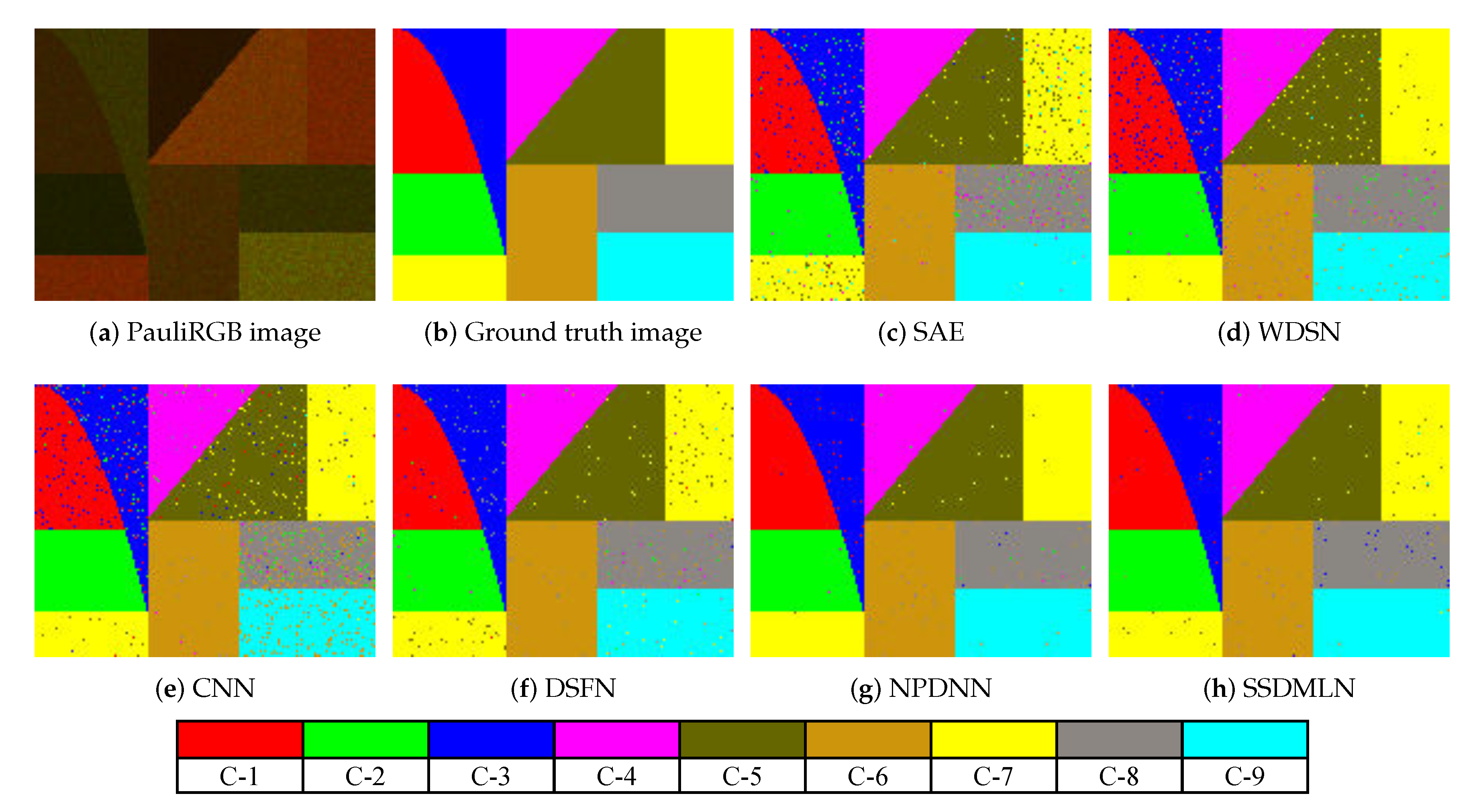
  • The synthetic data is obtained by the Monte-Carlo method ([25] Ch.4.5.2) with a size of 120 × 150 pixels, and it contains nine categories that are represented by C-1 to C-9, respectively.
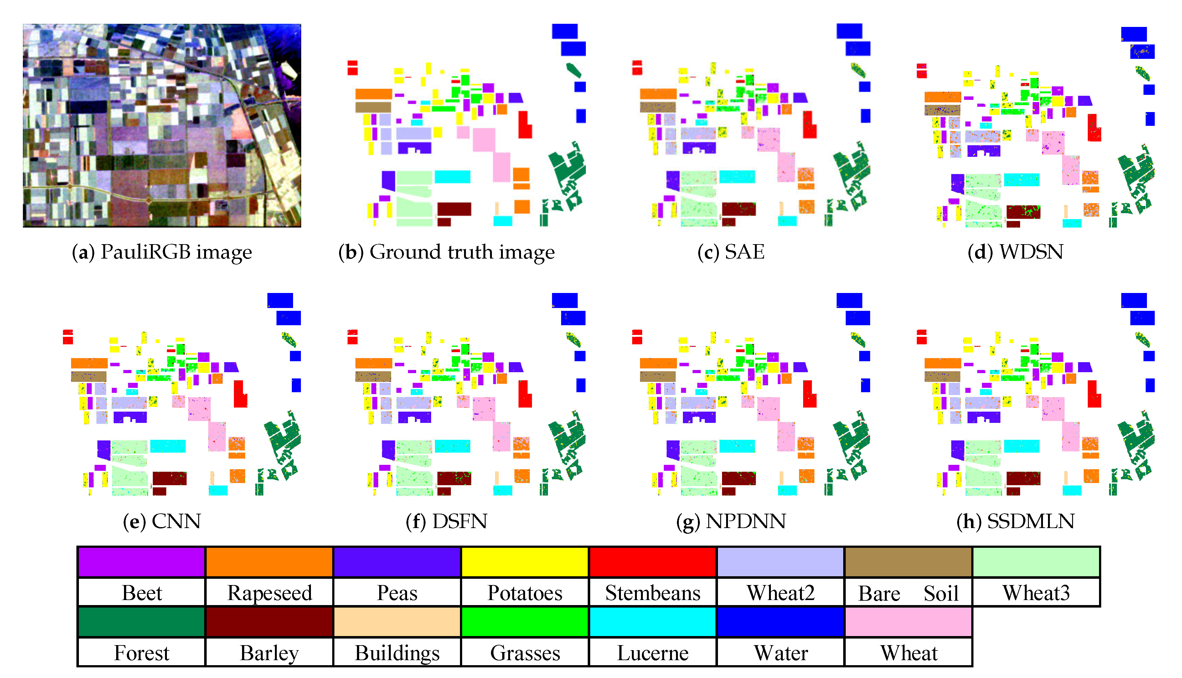
  • The Flevoland data set: This data set is acquired by the NASA/JPL AIRSAR system, and it is publicly available from the European Space Agency (ESA) (https://earth.esa.int/web/polsarpro/data-sources/sample-datasets). It is L-band four-look data, its resolution is 12 × 6 m, and the image size is 750 × 1024 pixels. It has 15 types of terrain: peas, stem beans, lucerne, forest, beet, potatoes, wheat, rapeseed, barley, bare soil, wheat2, grass, wheat3, buildings, and water.
  • The San Francisco data set: This data set is from the RADARSAT-2 system, which is also publicly available from the ESA (https://earth.esa.int/web/polsarpro/spaceborne-data-sources). It is a C-band single-look full-polarization SAR data. The image size is 1300 × 1300 pixels, which represents the bay of San Francisco with the golden gate bridge. It includes five classes: low-density urban, water, high-density urban, the developed, and vegetation.
  • The Xi’an data set: This data set is imagery of the Xi’an city in China, and it is also acquired by RADARSAT-2, which is purchased by our institution. A sub-region in the western region is selected for the experiment, and the image size is 512 × 512 pixels for our experiments.
Moreover, we implemented the following five algorithms, which are related and state-of-the-art ones for comparison. Among them, SAE [8] and WDSN [9] are both supervised classification methods with unsupervised pre-training. CNN [10] is a typical supervised neural network without pre-training, and both DSFN [16] and NPDNN [17] are semi-supervised methods.
The parameters for all the methods are listed below:
  • SAE [8]: The parameter for sparsity is between [ 0.05 , 0.09 ] for each layer; the parameter of the sparsity penalty is set to 1; the learning rate or step-size is between [ 0.1 , 0.9 ] .
  • WDSN [9]: This network has two hidden layers, and the number of nodes for each is 50 and 100, respectively; the thresholds τ 0 is [ 0.95 , 0.99 ] , and ρ 0 is 0; the window size is [ 3 , 5 ] ; and the learning rate is 0.01.
  • CNN [10]: The network includes two convolutional layers, one fully connected layer and two max-pooling layers; the sizes of the first and the second convolutional filters are 3 × 3 , and 2 × 2 , respectively; the size of pooling is 2 × 2 ; the momentum parameter is 0.9; the weight decay rate is 5 × 10 4 .
  • DSFN [16]: The rate of weight decay is chosen from the internal [ 1 × 10 4 , 1 × 10 3 ] .
  • NPDNN [17]: The nearest-neighbor number is chosen in the interval [ 10 , 20 ] and the parameter of regularization α is fixed at 1; the learning rate and weight decay rate are chosen in the range [ 0.01 , 0.1 ] .
  • The proposed SSDMLN: The learning rate is 0.2; the weight reduction factor is 5 × 10 6 , and dropout rate is 0.5; the number of nearest neighbors is between [ 5 , 30 ] , respectively.
Additionally, other parameters of all the methods are manually tuned to their best results according to the data sets. We run all the methods for 20 times, and report the overall accuracy (OA) on average. The implementations are on a computer in which the GPU is with 11GB memory. For each dataset, we randomly select 1% data as labeled samples, and the Lee filtering [26] with 5 × 5 window size is applied for preprocessing to reduce noise.

4.2. Parameter Analysis

The main parameters of SSDMLN are chosen by experience and experiments. We take the synthetic dataset as an example. The network includes five layers, and the numbers of nodes in the hidden layers are 25, 100, and 50, respectively. The parameters are shown as follows:
(1)
The weight coefficients λ 1 , λ 2 , λ 3 , and λ 4
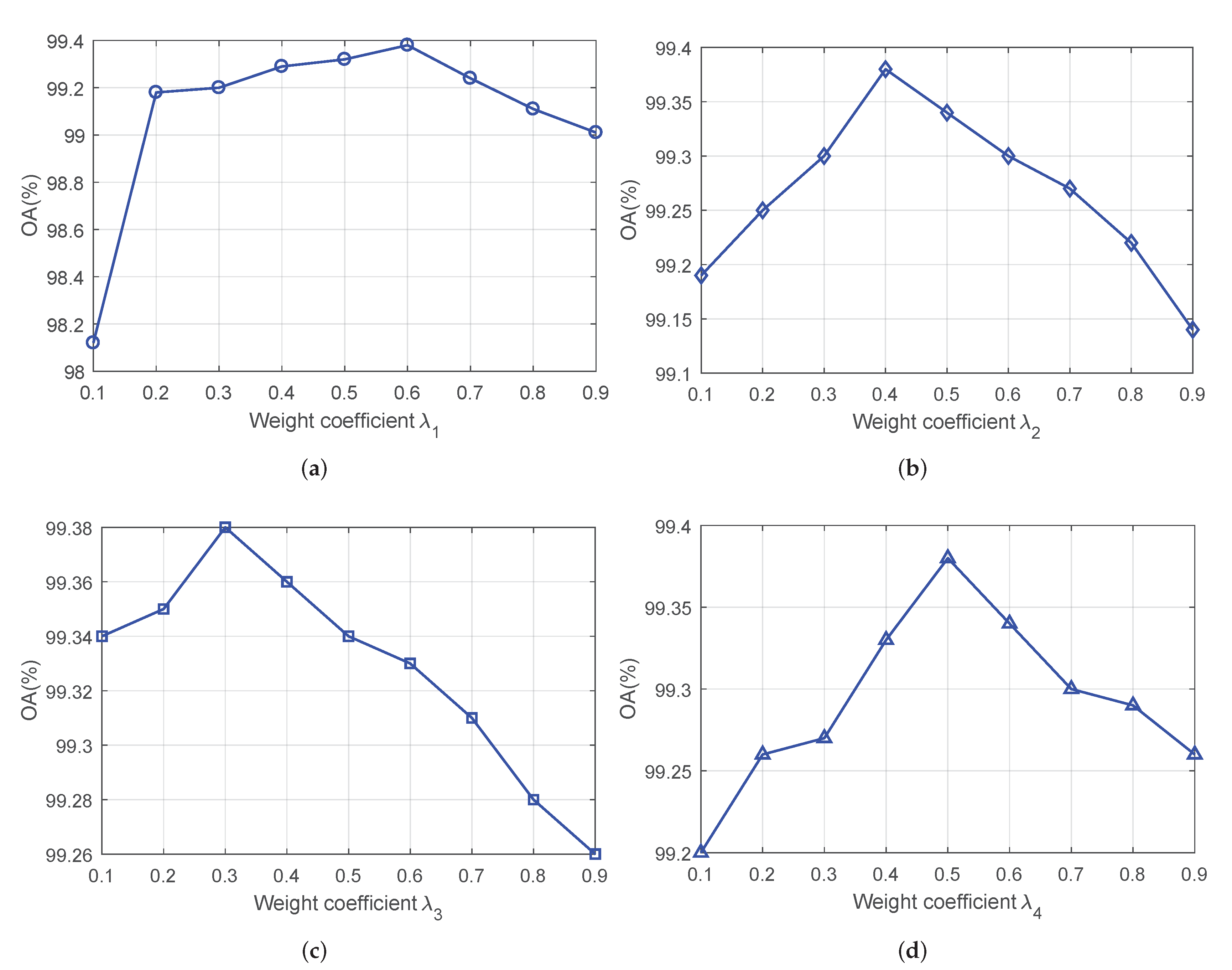
The coefficient λ 1 : The OA versus the varying parameter λ 1 is shown in Figure 2a, when we set λ 2 = 0.4 , λ 3 = 0.3 , and λ 4 = 0.5 , and the increasing step for λ 1 is 0.1. It indicates that when λ 1 is greater than 0.6, the OA falls. The accuracy for λ 1 = 0.6 is superior to the result at λ 1 = 0.5 . Therefore, the coefficient λ 1 should be set to 0.6 for this dataset.
The coefficient λ 2 : The OA versus the varying parameter λ 2 is shown in Figure 2b, when we set λ 1 = 0.6 , λ 3 = 0.3 , and λ 4 = 0.5 . It indicates that the coefficient λ 2 should be set to 0.4 for this dataset.
The coefficient λ 3 : The OA versus the varying parameter λ 3 is shown in Figure 2c, when we set λ 1 = 0.6 , λ 2 = 0.4 , and λ 4 = 0.5 . It indicates that the coefficient λ 3 should be set to 0.3 for this dataset.
The coefficient λ 4 : The OA versus the varying parameter λ 4 is shown in Figure 2d, when we set λ 1 = 0.6 , λ 2 = 0.4 , and λ 3 = 0.3 . It indicates that the coefficient λ 4 should be set to 0.5 for this dataset.
(2)
The number of nearest neighbors K
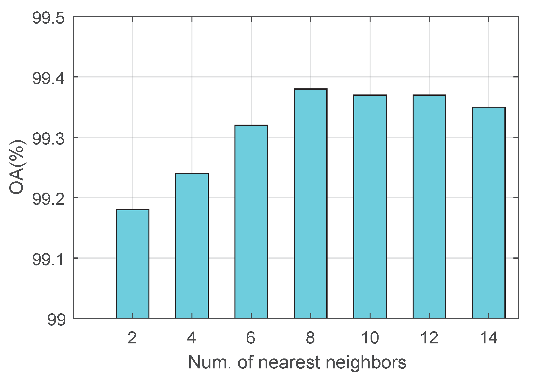
The classification accuracies vary with the number of nearest neighbors K, which is shown in Figure 3. It indicates that K is set 8 for this data set.

4.3. Experimental Results

(1) The synthetic dataset is shown in Figure 4a,b, and classification results by different algorithms on this dataset are demonstrated in Figure 4c–h. It shows that our SSDMLN attains the best visual result for each class, and the misclassified pixels are much fewer than those of other algorithms, even if for the curved boundary on the left of the image. It also indicates that SSDMLN has fine capability for division of non-linear boundary, which may benefit from the layer-wise feature learning. The overall accuracies are shown in Table 1. It demonstrates that the OA of SSDMLN is highest at 99.38%, which is better than state-of-the-art semi-supervised networks including DSFN and NPDNN. It is likely that the class discriminative information for SSDMLN plays a role in the layer-by-layer learning. Although CNN has been reported satisfactory performance for many pattern recognition tasks, it is inferior to other networks, such as SAE, WDSN and NPDNN, on this dataset. The main reason for these semi-supervised approaches obtaining high accuracies with only 1% labeled samples is that they make good use of prior knowledge from unlabeled samples, while the supervised CNN may be overfitting and works poorly with insufficient labeled samples.
(2) Classification results by different algorithms on the Flevoland dataset are given in Figure 5c–h. It is obvious that our SSDMLN has a satisfactory visual result compared with that of other algorithms. The reason is because our algorithm exploits the information from both the few labeled pixels and large quantities of unlabeled pixels with metric learning. The classification accuracies are listed in Table 2. SSDMLN obtains the highest OA, and it reaches 94.85%. Especially for stembeans, potatoes, peas, lucerne, barley, grass, and water, it achieves the highest accuracy. On the contrary, the semi-supervised DSFN and NPDNN have lower accuracies for these terrains, and SAE and WDSN, which are based on the unsupervised pre-training, perform poorly with 1% labeled samples. This also indicates that our proposed metric learning-based network has a robust distinguishing ability for homogenous terrain.
(3) Classification results by different algorithms on the San Francisco dataset are demonstrated in Figure 6c–h. It can be seen that the visual result of SSDMLN is still the best among the other algorithms, especially on the low-density urban area, which is challenging to categorize for this heterogeneous terrain. Moreover, the classification accuracies are listed in Table 3. SSDMLN still attains the highest OA, and it achieves an increase of 8% and 7% compared with WDSN and CNN, respectively. Especially on the low-density urban and the developed area, it is nearly 20% higher than other algorithms. The reason for the low accuracy of WDSN and CNN is that the labeled samples are quite limited for their training. Nevertheless, on one side, SSDMLN utilizes metric learning to increase the discriminative ability of classes, and on the other, it uses manifold regularization to decrease the dependence on labeled data.
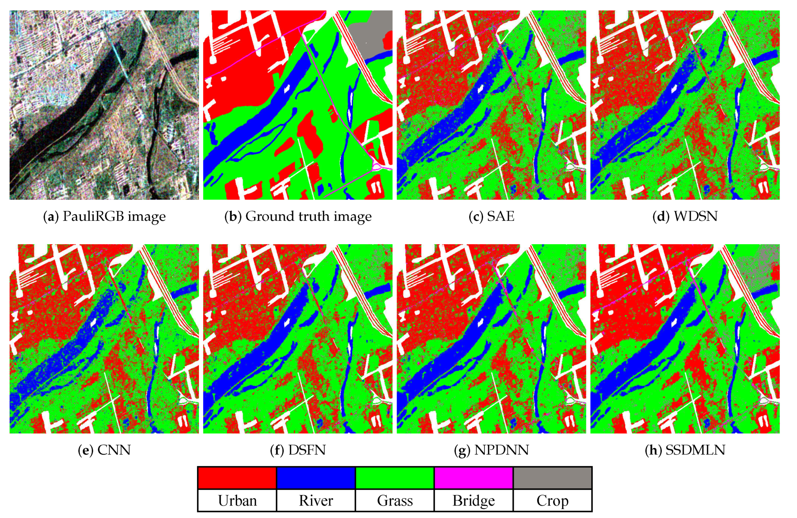
(4) The Classification results generated by all the algorithms on the Xi’an data set are illustrated in Figure 7c–h. The original image in RGB is reported in Figure 7a. The urban regions, where there are many build-ups, are mainly on the left. The River Weihe is in the middle of the image, and it is one primary branch of Yellow River in China. The Weihe Bridge spans the River Weihe. A railway also spans the river. The grass and the trees are around the rivers. Figure 7b shows the ground truth. Reference data were collected from aerial photographic interpretation, Google satellite images and the fieldwork. The visual results demonstrate that SSDMLN is superior to other algorithms. Furthermore, the overall accuracies are reported in Table 4. It indicates that SSDMLN obtains the highest accuracy not only for the terrain of urban, river and grass, which have relatively more samples, but also for the terrain of the bridge and crop, which are of much fewer samples in total. Especially for the bridge, SSDMLN has an accuracy of 34.30%, which is significantly higher than that of the other algorithms. It indicates that SSDMLN can identify the classes with very few labeled samples. It is probably because the metric learning together with the manifold regularization takes full advantage of lots of unlabeled pixels, and thus reduces the dependence on labeled pixels.
In fact, there are really significant differences in the classification accuracies on the studied datasets. This is likely because the datasets from different radar systems have different characteristics (e.g., in terms of imaging mode, noise level, the observed target, etc.), which can bring a significant difference in the classification results. This phenomenon also appears in other research work (e.g., [10,11,14]). It may be data driven, and the performance of the presented model can be exactly repetitive, since in our studies, we run each classification experiment for 20 times. One can draw similar results as presented in our paper.

5. Conclusions

A novel semi-supervised deep metric learning network (SSDMLN) was proposed for the classification of PolSAR data in this work. The metric learning is utilized to construct a layer-wise network, which transforms the linear mapping to the non-linear projection for learning the intuitive features from PolSAR data. Meanwhile, we presented a manifold regularization to make full use of unlabeled samples, which can reduce the distance between neighboring samples. The extensive experiments on both synthetic and real-world datasets demonstrated the effectiveness of the proposed network compared with existing methods. The strengths of our SSDMLN method were also confirmed by extensive experimental results: (1) The linear metric learning embedded in the non-linear network can extract intuitive features and thus improves the classification performance for both heterogeneous and homogenous terrains. (2) During the layer-wise learning, our manifold regularization is very effective for semi-supervised learning, which cuts down the number of labeled samples for classification. This provides inspirations for the design of semi-supervised deep neural networks for other research work. It is noticed that the method for selection of weight coefficients is not optimal. In the future, more sophisticated methodologies, such as random search [27] and gradient-based search [28], will be studied to tune the weight coefficients in various real-world applications.

Author Contributions

Conceptualization and methodology, H.L. and F.S.; writing, R.L., X.M., S.G. and B.H. All authors have read and agreed to the published version of the manuscript.

Funding

This research was funded by the National Natural Science Foundation of China (Nos. 61876220, 61876221, 61976164, 61836009 and U1701267), the Project supported the Foundation for Innovative Research Groups of the National Natural Science Foundation of China (No. 61621005), the Program for Cheung Kong Scholars and Innovative Research Team in University (No. IRT_15R53), the Fund for Foreign Scholars in University Research and Teaching Programs (the 111 Project) (No. B07048), the Science Foundation of Xidian University (Nos. 10251180018 and 10251180019), the National Science Basic Research Plan in Shaanxi Province of China (Nos. 2019JQ-657 and 2020JM-194), and the Key Special Project of China High Resolution Earth Observation System-Young Scholar Innovation Fund. Jun Fan was supported by the Natural Science Foundation of Hebei Province (No. A2019202135).

Acknowledgments

We thank the reviewers for their valuable comments.

Conflicts of Interest

The authors declare no conflict of interest.

References

  1. Lee, J.S.; Grunes, M.R.; Ainsworth, T.L.; Du, L.J.; Schuler, D.L.; Cloude, S.R. Unsupervised classification using polarimetric decomposition and the complex Wishart classifier. IEEE Trans. Geosci. Remote Sens. 1999, 37, 2249–2258. [Google Scholar]
  2. Du, L.; Lee, J. Fuzzy classification of earth terrain covers using complex polarimetric SAR data. Int. J. Remote Sens. 1996, 17, 809–826. [Google Scholar] [CrossRef]
  3. Lee, J.S.; Grunes, M.R.; Pottier, E.; Ferro-Famil, L. Unsupervised terrain classification preserving polarimetric scattering characteristics. IEEE Trans. Geosci. Remote Sens. 2004, 42, 722–731. [Google Scholar]
  4. Liu, H.; Wang, S.; Wang, R.; Shi, J.; Zhang, E.; Yang, S.; Jiao, L. A framework for classification of urban areas using polarimetric SAR images integrating color features and statistical model. Int. J. Infrared Millim. Waves 2016, 35, 398–406. [Google Scholar]
  5. Fukuda, S.; Hirosawa, H. Polarimetric SAR image classification using support vector machines. IEICE Trans. Inf. Syst. 2001, 84, 1939–1945. [Google Scholar]
  6. Lardeux, C.; Frison, P.L.; Tison, C.; Souyris, J.C.; Stoll, B.; Fruneau, B.; Rudant, J.P. Support vector machine for multifrequency SAR polarimetric data classification. IEEE Trans. Geosci. Remote Sens. 2009, 47, 4143–4152. [Google Scholar] [CrossRef]
  7. Zou, T.; Yang, W.; Dai, D.; Sun, H. Polarimetric SAR image classification using multifeatures combination and extremely randomized clustering forests. EURASIP J. Adv. Signal Process. 2010, 2010, 465612. [Google Scholar] [CrossRef] [Green Version]
  8. Xie, H.; Wang, S.; Liu, K.; Lin, S.; Hou, B. Multilayer feature learning for polarimetric synthetic radar data classification. In Proceedings of the 2014 IEEE Geoscience and Remote Sensing Symposium, Quebec City, QC, Canada, 13–18 July 2014; pp. 2818–2821. [Google Scholar]
  9. Jiao, L.; Liu, F. Wishart deep stacking network for fast POLSAR image classification. IEEE Trans. Image Process. 2016, 25, 3273–3286. [Google Scholar] [CrossRef]
  10. Zhou, Y.; Wang, H.; Xu, F.; Jin, Y.Q. Polarimetric SAR image classification using deep convolutional neural networks. IEEE Geosci. Remote Sens. Lett. 2016, 13, 1935–1939. [Google Scholar] [CrossRef]
  11. Wei, B.; Yu, J.; Wang, C.; Wu, H.; Li, J. PolSAR image classification using a semi-supervised classifier based on hypergraph learning. Remote Sens. Lett. 2014, 5, 386–395. [Google Scholar] [CrossRef]
  12. Liu, H.; Wang, Y.; Yang, S.; Wang, S.; Feng, J.; Jiao, L. Large polarimetric SAR data semi-supervised classification with spatial-anchor graph. IEEE J. Sel. Top. Appl. Earth Obs. Remote Sens. 2016, 9, 1439–1458. [Google Scholar] [CrossRef]
  13. Liu, H.; Yang, S.; Gou, S.; Liu, S.; Jiao, L. Terrain classification based on spatial multi-attribute graph using polarimetric SAR data. Appl. Soft Comput. 2018, 68, 24–38. [Google Scholar] [CrossRef]
  14. Li, Y.; Xing, R.; Jiao, L.; Chen, Y.; Chai, Y.; Marturi, N.; Shang, R. Semi-Supervised PolSAR Image Classification Based on Self-Training and Superpixels. Remote Sens. 2019, 11, 1933. [Google Scholar] [CrossRef] [Green Version]
  15. Hua, W.; Wang, S.; Liu, H.; Liu, K.; Guo, Y.; Jiao, L. Semisupervised PolSAR image classification based on improved cotraining. IEEE J. Sel. Top. Appl. Earth Obs. Remote Sens. 2017, 10, 4971–4986. [Google Scholar] [CrossRef]
  16. Liu, H.; Min, Q.; Sun, C.; Zhao, J.; Yang, S.; Hou, B.; Feng, J.; Jiao, L. Terrain classification with polarimetric SAR based on deep sparse filtering network. In Proceedings of the 2016 IEEE International Geoscience and Remote Sensing Symposium (IGARSS), Beijing, China, 10–15 July 2016; pp. 64–67. [Google Scholar]
  17. Liu, H.; Yang, S.; Gou, S.; Zhu, D.; Wang, R.; Jiao, L. Polarimetric SAR feature extraction with neighborhood preservation-based deep learning. IEEE J. Sel. Top. Appl. Earth Obs. Remote Sens. 2017, 10, 1456–1466. [Google Scholar] [CrossRef]
  18. Yang, L.; Jin, R. Distance Metric Learning: A Comprehensive Survey; Michigan State Universiy: East Lansing, MI, USA, 2006; Volume 2, p. 4. [Google Scholar]
  19. Kulis, B. Metric Learning: A Survey. Found. Trends Mach. Learn. 2013, 5, 287–364. [Google Scholar] [CrossRef]
  20. Weinberger, K.Q.; Saul, L.K. Distance metric learning for large margin nearest neighbor classification. J. Mach. Learn. Res. 2009, 10, 207–244. [Google Scholar]
  21. Liu, H.; Zhu, D.; Yang, S.; Hou, B.; Gou, S.; Xiong, T.; Jiao, L. Semisupervised feature extraction with neighborhood constraints for polarimetric SAR classification. IEEE J. Sel. Top. Appl. Earth Obs. Remote Sens. 2016, 9, 3001–3015. [Google Scholar] [CrossRef]
  22. Liu, H.; Shang, F.; Yang, S.; Gong, M.; Zhu, T.; Jiao, L. Sparse Manifold-Regularized Neural Networks for Polarimetric SAR Terrain Classification. IEEE Trans. Neural Netw. Learn. Syst. 2019. [Google Scholar] [CrossRef]
  23. Liu, H.; Wang, F.; Yang, S.; Biao, H.; Licheng, J.; Yang, R. Fast Semi-supervised Classification Using Histogram-based Density Estimation for Large-scale Polarimetric SAR Data. IEEE Geosci. Remote Sens. 2019, 16, 1844–1848. [Google Scholar] [CrossRef]
  24. Liu, H.; Wang, Z.; Shang, F.; Yang, S.; Gou, S.; Licheng, J. Semi-supervised Tensorial Locally Linear Embedding for Feature Extraction using PolSAR Data. IEEE J-STSP 2018, 12, 1476–1490. [Google Scholar] [CrossRef]
  25. Lee, J.S.; Pottier, E. Polarimetric Radar Imaging: From Basics to Applications; CRC Press: Boca Raton, FL, USA, 2009. [Google Scholar]
  26. Lee, J.S.; Grunes, M.; de Grandi, G. Polarimetric SAR speckle filtering and its implication for classification. IEEE Trans. Geosci. Remote Sens. 1999, 37, 2363–2373. [Google Scholar]
  27. Bergstra, J.; Bengio, Y. Random search for hyper-parameter optimization. JMLR 2012, 13, 281–305. [Google Scholar]
  28. Beng, Y. Gradient-based optimization of hyperparameters. Neural Comput. 2000, 12, 1889–1900. [Google Scholar] [CrossRef]
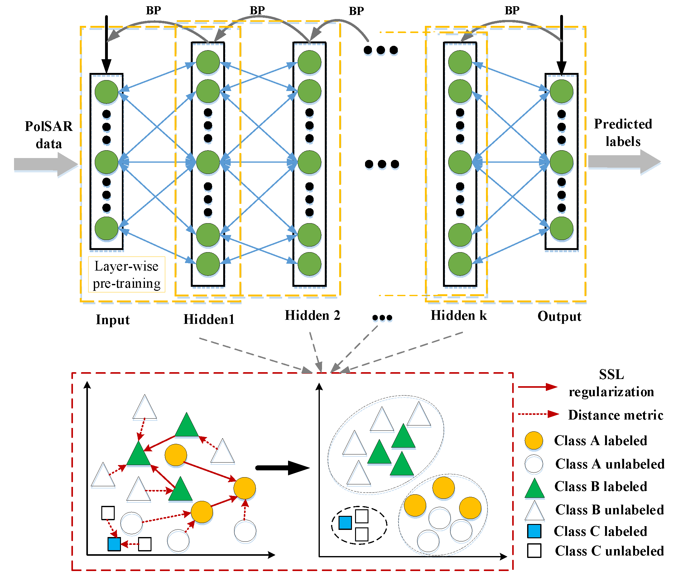
Figure 1. The architecture of our semi-supervised deep metric learning network (SSDMLN).
Remotesensing 12 01593 g001
Figure 2. Classification accuracy versus different weight coefficients on the synthetic PolSAR dataset. (a) λ 1 , (b) λ 2 , (c) λ 3 , (d) λ 4 .
Remotesensing 12 01593 g002
Figure 3. The overall accuracy varies with the number of nearest neighbors on the synthetic PolSAR data set.
Remotesensing 12 01593 g003
Figure 4. Comparison of classification results on the synthetic data set using 1% labeled data. (a) PauliRGB image. (b) Ground truth image. (c) SAE [8]. (d) WDSN [9]. (e) CNN [10]. (f) DSFN [16]. (g) NPDNN [17]. (h) SSDMLN (ours).
Remotesensing 12 01593 g004
Figure 5. Comparison of classification results on the Flevoland data set using 1% labeled data. (a) PauliRGB image. (b) Ground truth image. (c) SAE [8]. (d) WDSN [9]. (e) CNN [10]. (f) DSFN [16]. (g) NPDNN [17]. (h) SSDMLN (ours).
Remotesensing 12 01593 g005
Figure 6. Comparison of classification results on the San Francisco data set using 1% labeled data. (a) PauliRGB image. (b) Ground truth. (c) SAE [8]. (d) WDSN [9]. (e) CNN [10]. (f) DSFN [16]. (g) NPDNN [17]. (h) SSDMLN (ours).
Remotesensing 12 01593 g006
Figure 7. Comparison of classification results on the Xi’an data set using 1% labeled data. (a) PauliRGB image. (b) Ground truth. (c) SAE [8]. (d) WDSN [9]. (e) CNN [10]. (f) DSFN [16]. (g) NPDNN [17]. (h) SSDMLN (ours).
Remotesensing 12 01593 g007
Table 1. Classification results (%) on the synthetic data set with 1% labeled data where C-1 to C-9 denote 9 different categories.
MethodsC-1C-2C-3C-4C-5C-6C-7C-8C-9OA
SAE [8]96.1499.4792.36100.098.7298.9992.5792.2199.6696.15
WDSN [9]95.3798.3689.5697.2194.3889.7689.3290.4791.8992.36
CNN [10]95.81100.090.8897.8295.2698.5198.6585.1590.2694.17
DSFN [16]98.6198.8494.3399.9597.6891.1497.7098.7099.3297.80
NPDNN [17]98.7799.8596.8099.9598.8194.9899.3598.3799.4998.70
SSDMLN (ours)99.7499.9399.0299.6999.6098.6698.9898.5299.8199.38
Table 2. Classification results (%) on the Flevoland data set with 1 % labeled data.
MethodsSAE [8]WDSN [9]CNN [10]DSFN [16]NPDNN [17]SSDMLN (ours)
Peas93.3680.4285.1593.1595.3096.32
Stembeans93.2562.5593.4796.5696.0196.62
Lucerne92.1188.3170.1091.5794.1095.49
Forest87.8388.4599.8891.9693.0392.03
Beet94.3580.2199.7295.2596.1596.80
Potatoes87.0785.5391.2090.2691.0292.39
Wheat90.2479.6694.9991.5690.4692.57
Rapeseed83.1676.3297.6689.0488.4689.94
Bare Soil94.5487.8997.6893.1497.7097.54
Wheat279.8279.3484.9788.9689.1087.82
Grasses73.1178.0645.2090.5382.5893.08
Wheat390.8689.6599.8190.2595.1094.60
Barley94.9767.2433.6794.1694.8397.40
Buildings87.5986.3587.3591.2490.3592.62
Water99.0895.1188.1993.1098.5499.42
OA88.1283.4188.1292.2593.5794.85
Table 3. Classification results (%) on San Francisco data set with 1 % labeled data.
MethodsWaterVegetationL-UrbanH-UrbanDevelopedOA
SAE [8]98.9483.1455.8585.7863.4487.95
WDSN [9]98.2876.3553.1182.2366.4886.41
CNN [10]98.8481.7053.7185.3162.2887.96
DSFN [16]99.9091.6255.9286.4668.5990.00
NPDNN [17]99.9491.7469.7087.9574.8592.36
SSDMLN (ours)99.9893.5575.9191.1581.2394.49
Table 4. Classification results (%) on the Xi’an data set with 1 % labeled data.
MethodsUrbanRiverGrassBridgeCropOA
SAE [8]74.1982.8575.0526.1918.3072.59
WDSN [9]74.5883.6873.3316.3815.9571.69
CNN [10]75.5476.0174.2385.3112.1271.40
DSFN [16]77.0186.6880.7917.3113.7876.48
NPDNN [17]79.0387.3780.1127.3915.6477.14
SSDMLN (ours)84.4386.7780.5934.3040.1382.10