Small Scale Landslide Detection Using Sentinel-1 Interferometric SAR Coherence


Abstract
:
1. Introduction
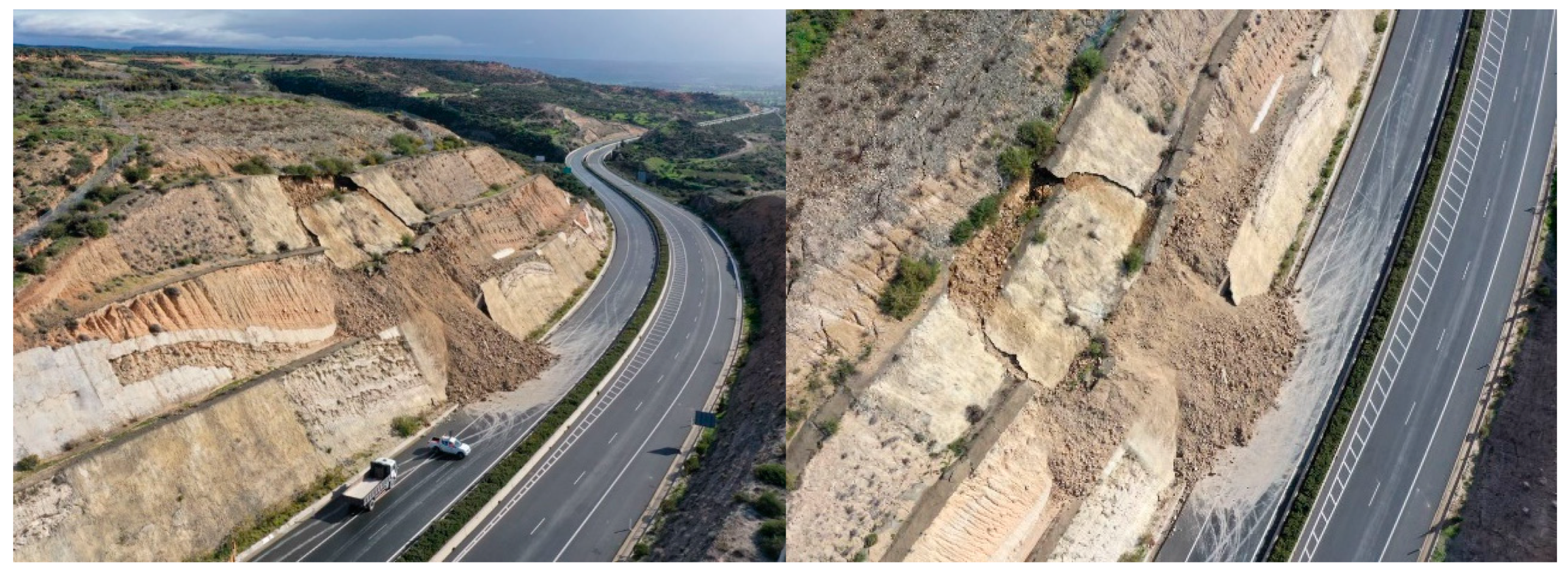
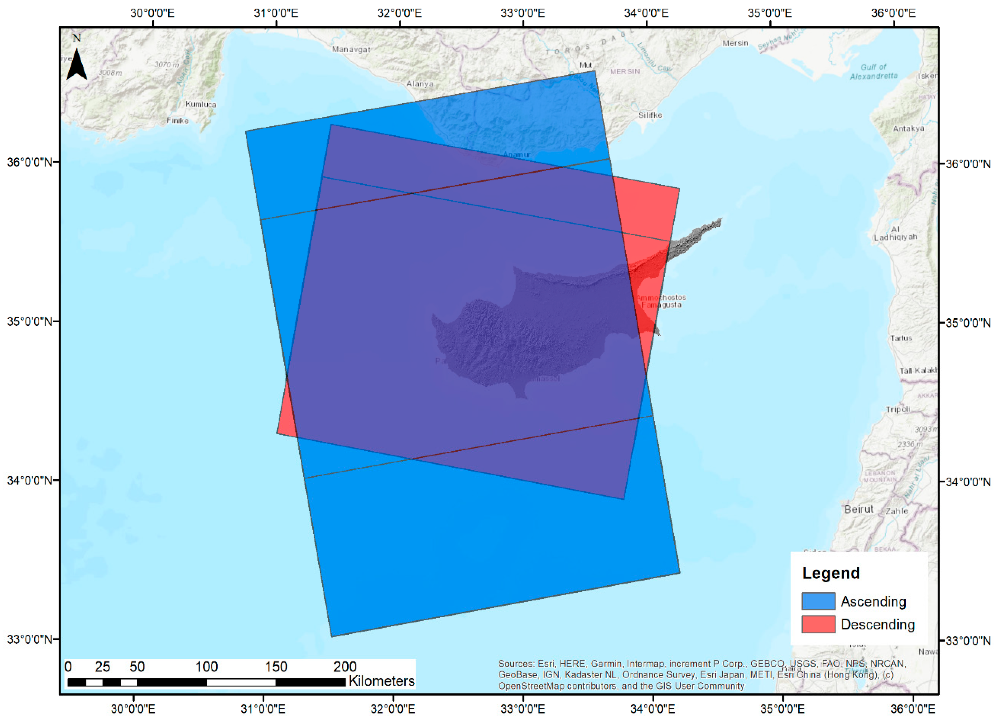
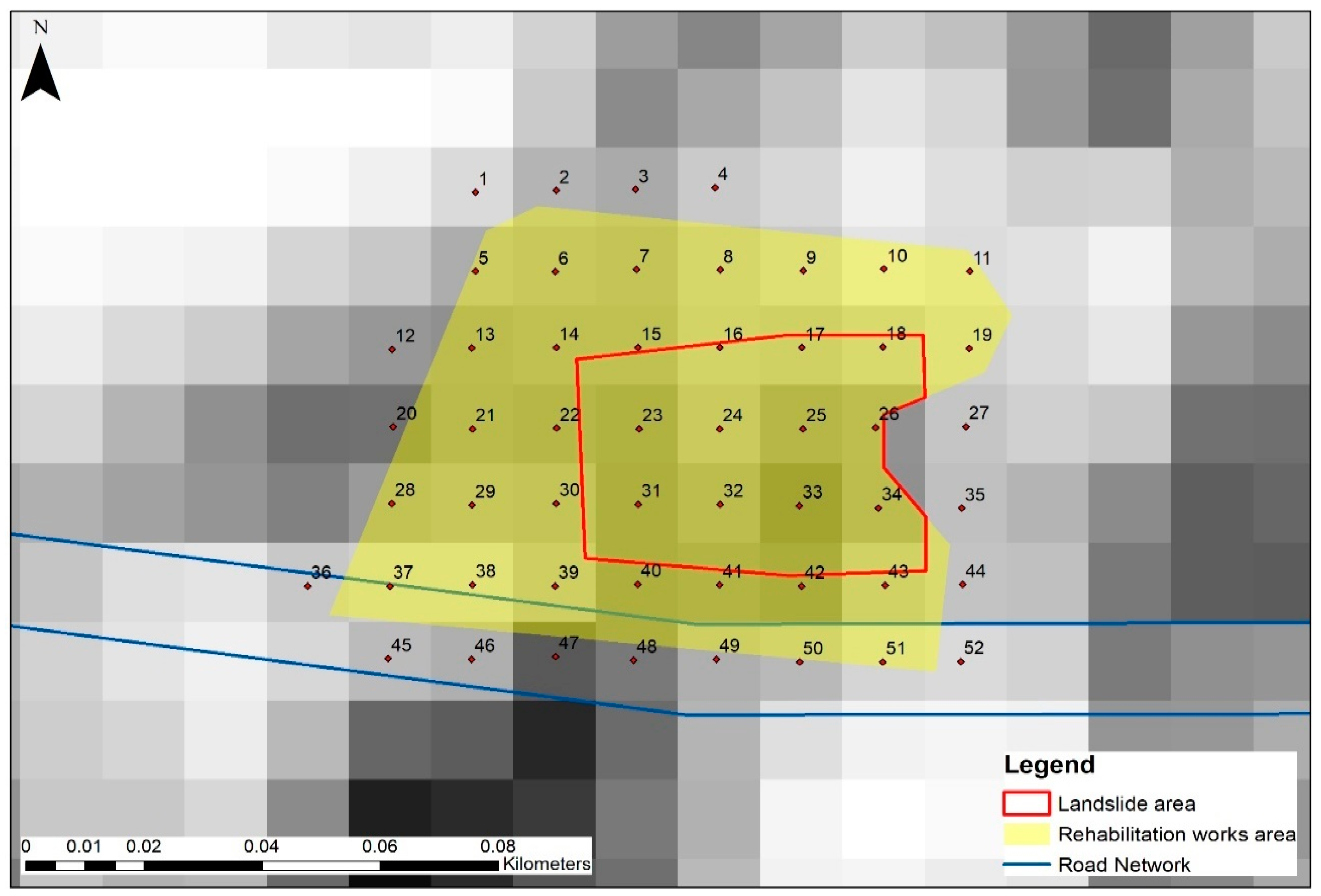
2. Area of Study
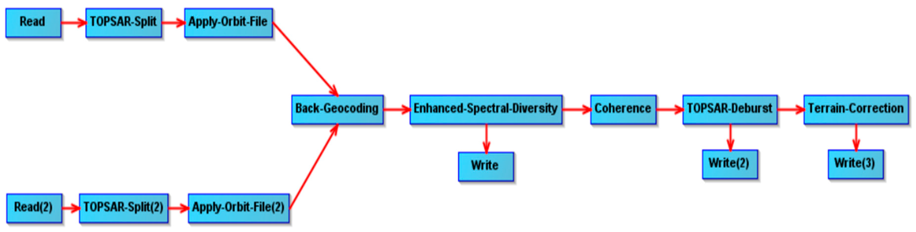
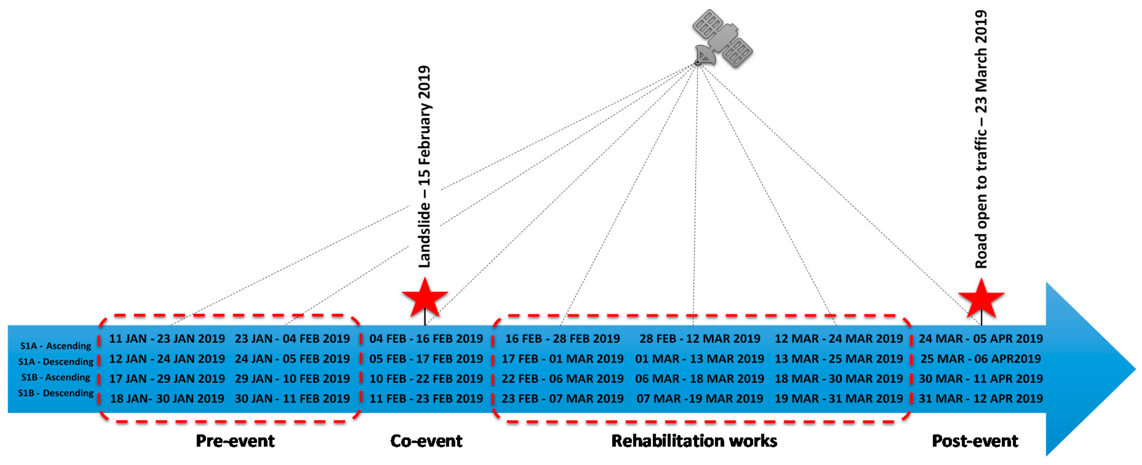
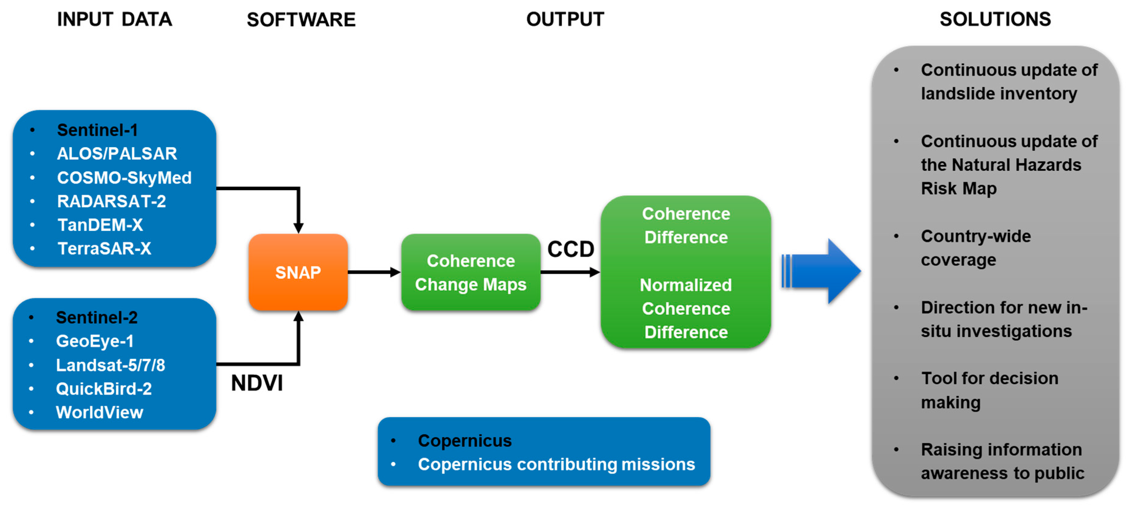
3. Materials and Methods
4. Results
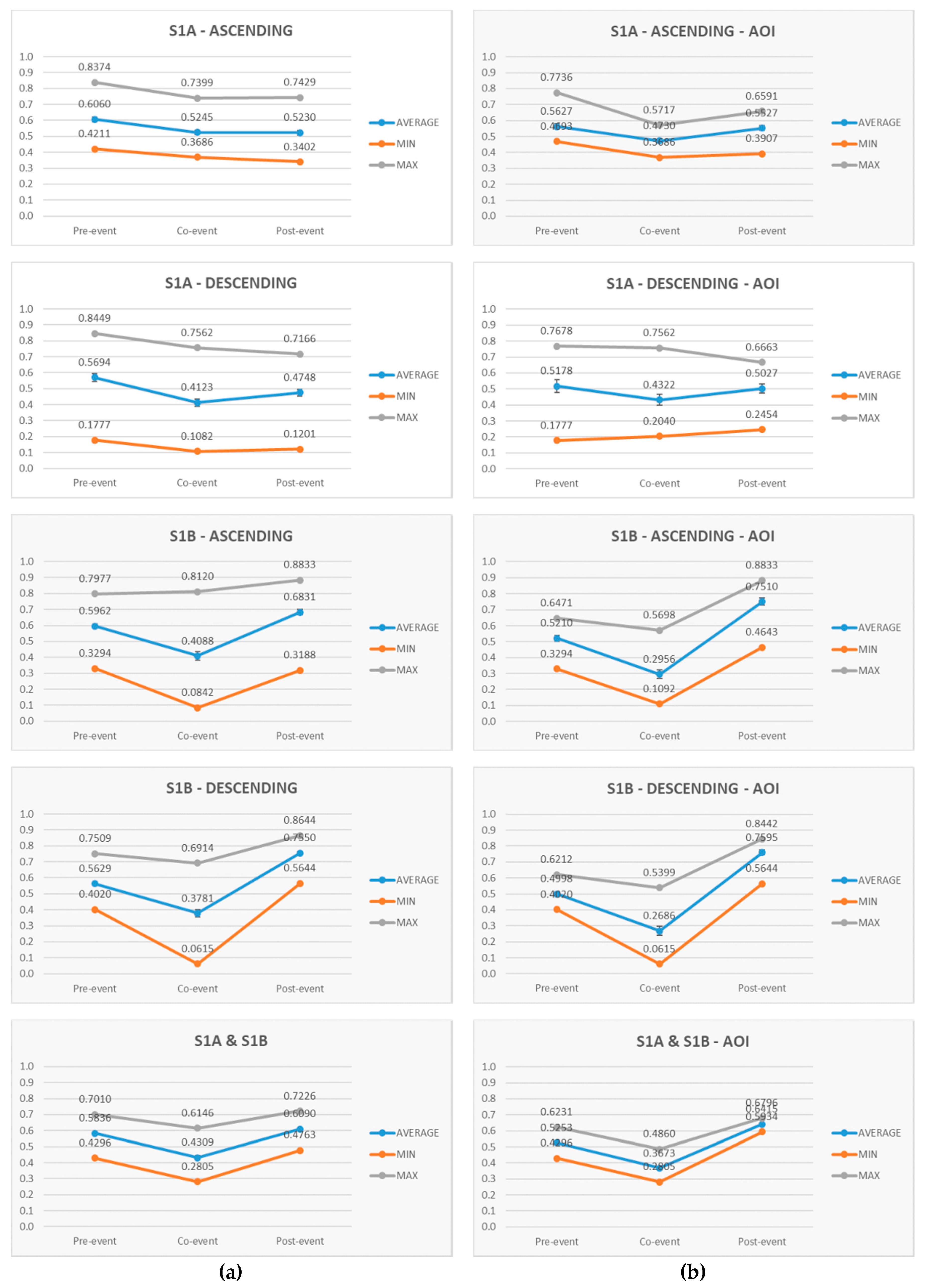
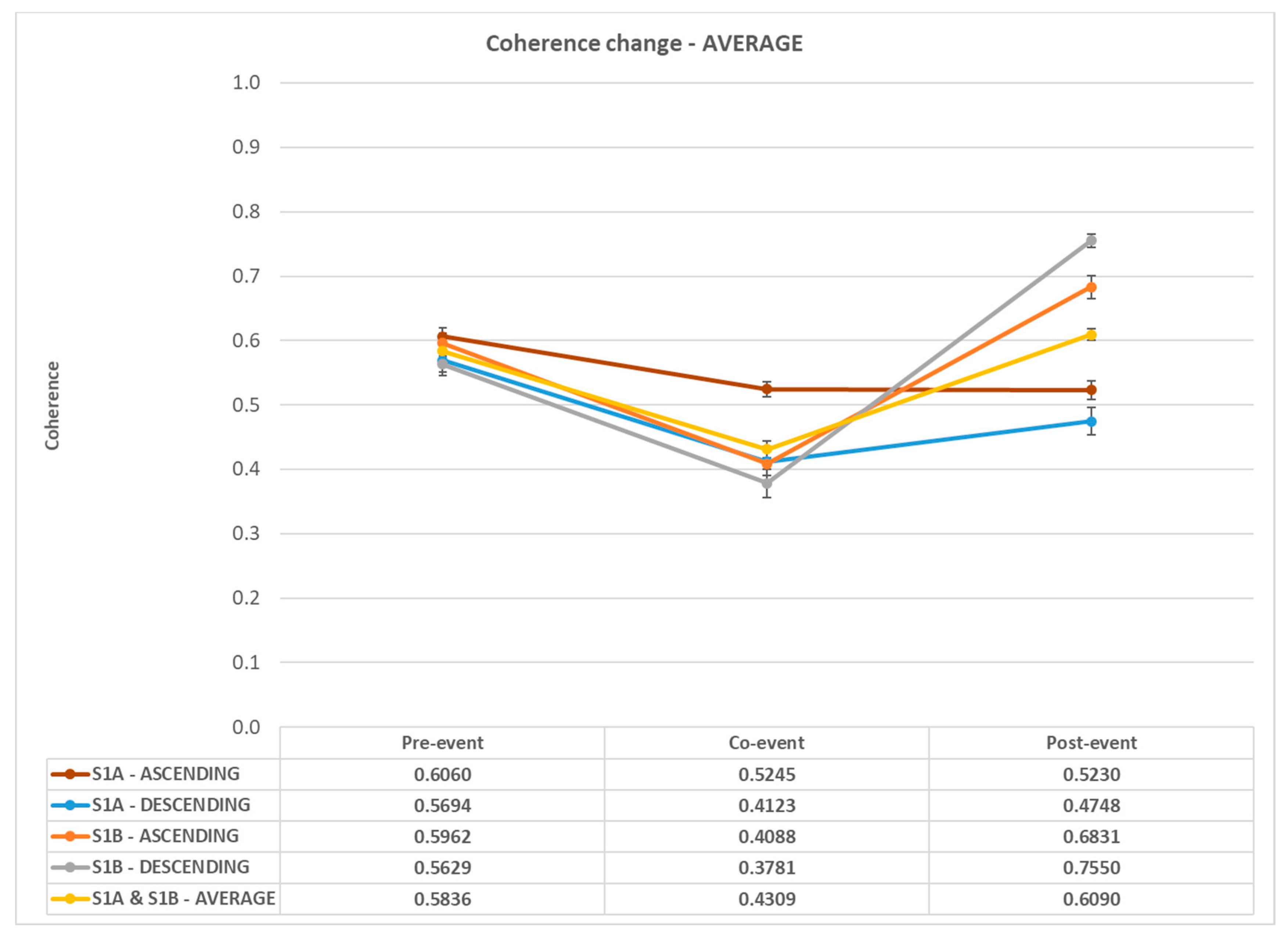
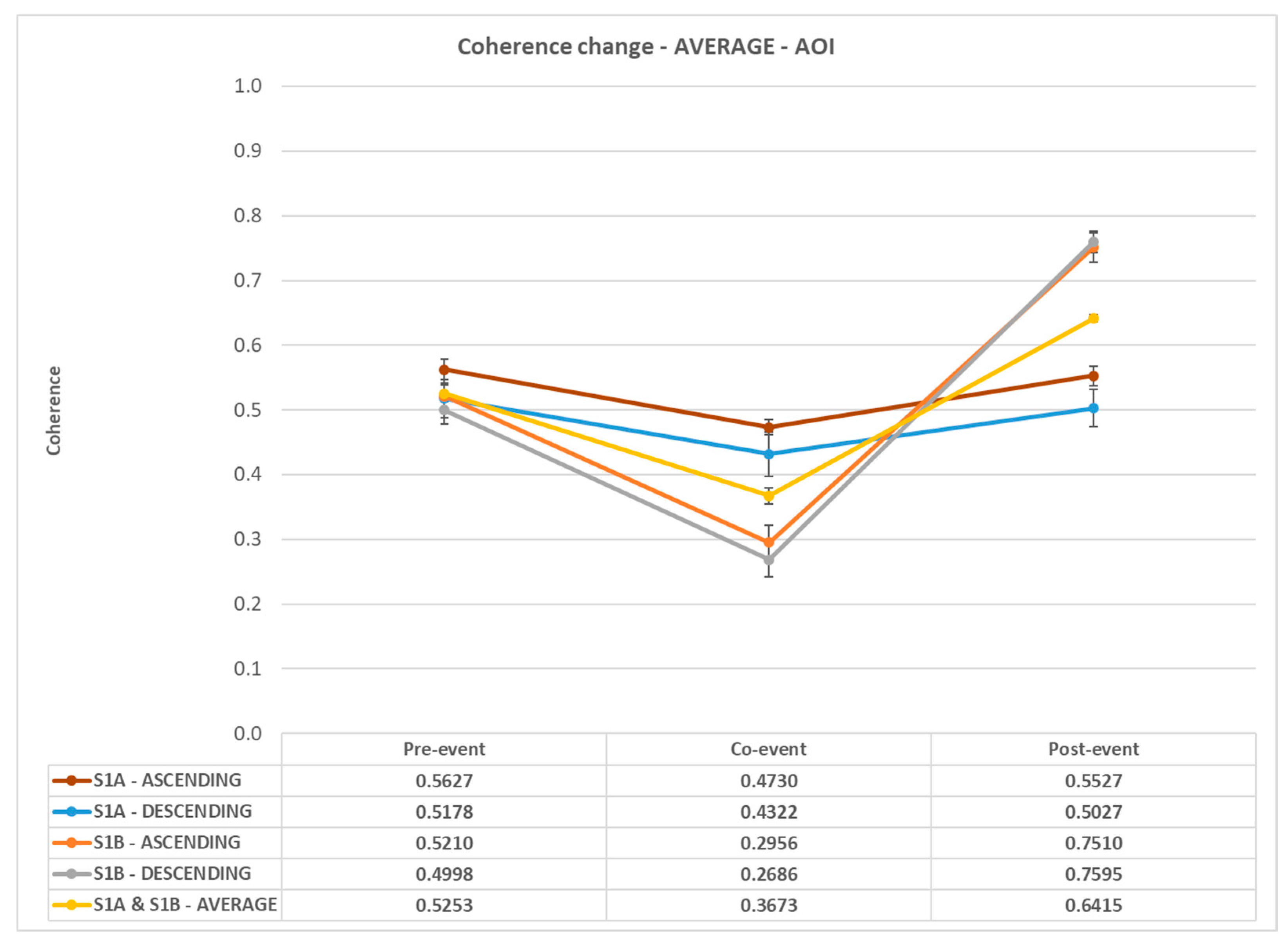
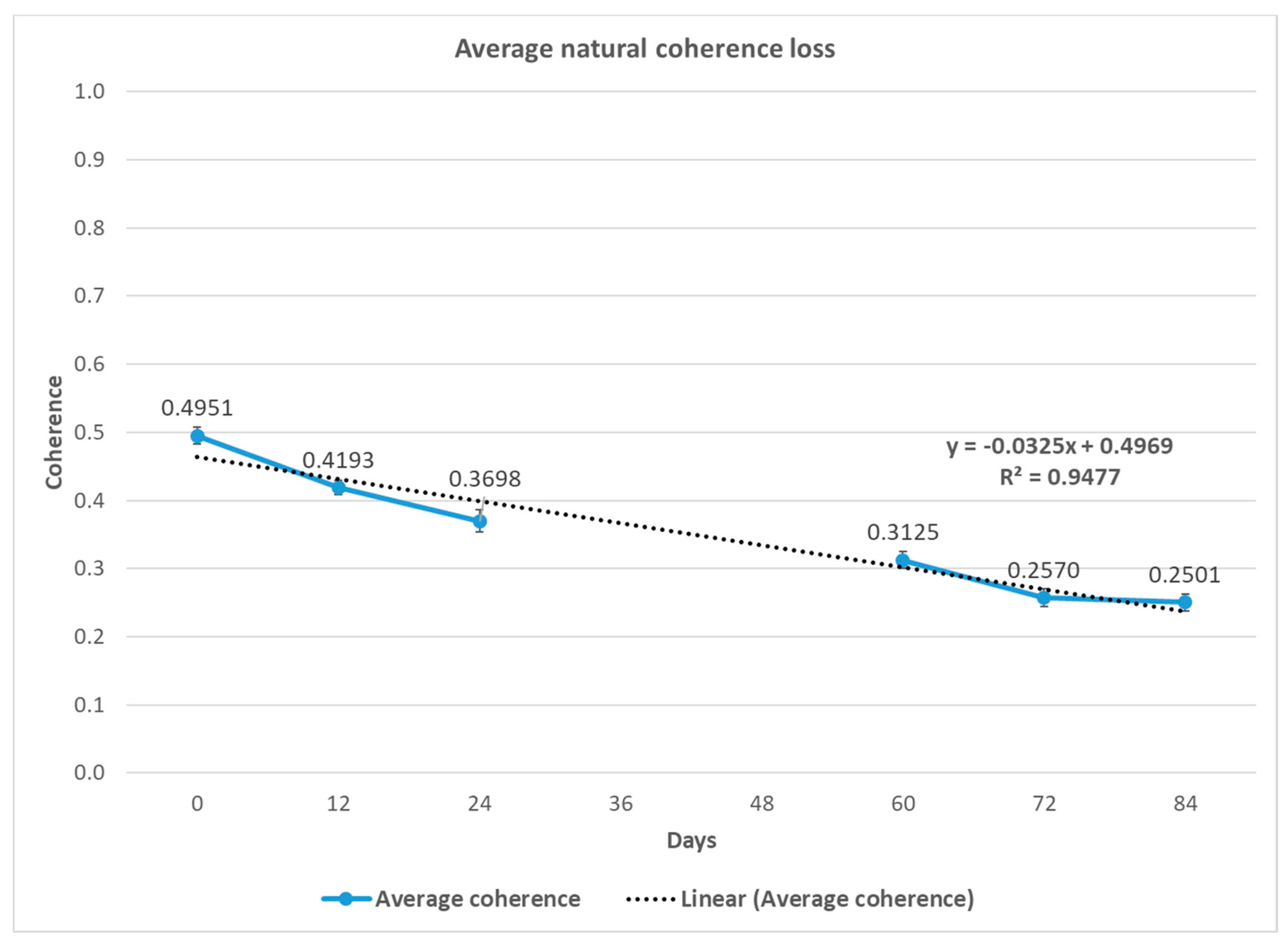
4.1. Statistical Analysis
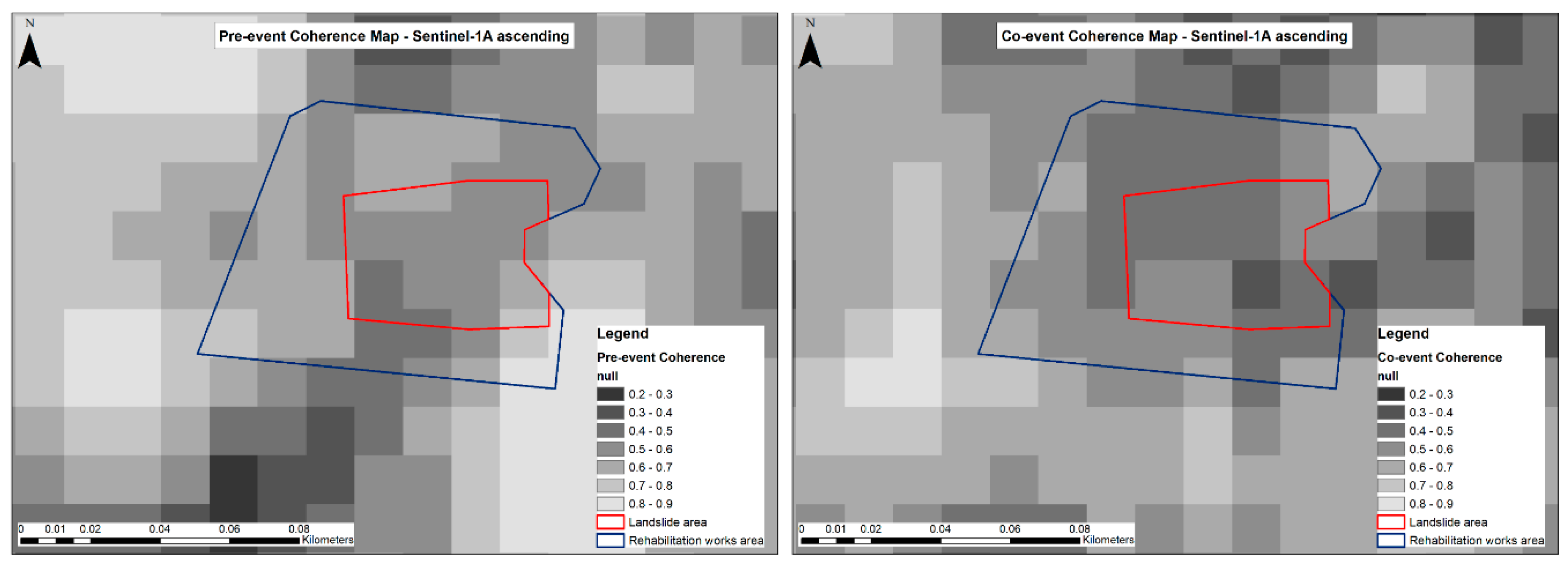
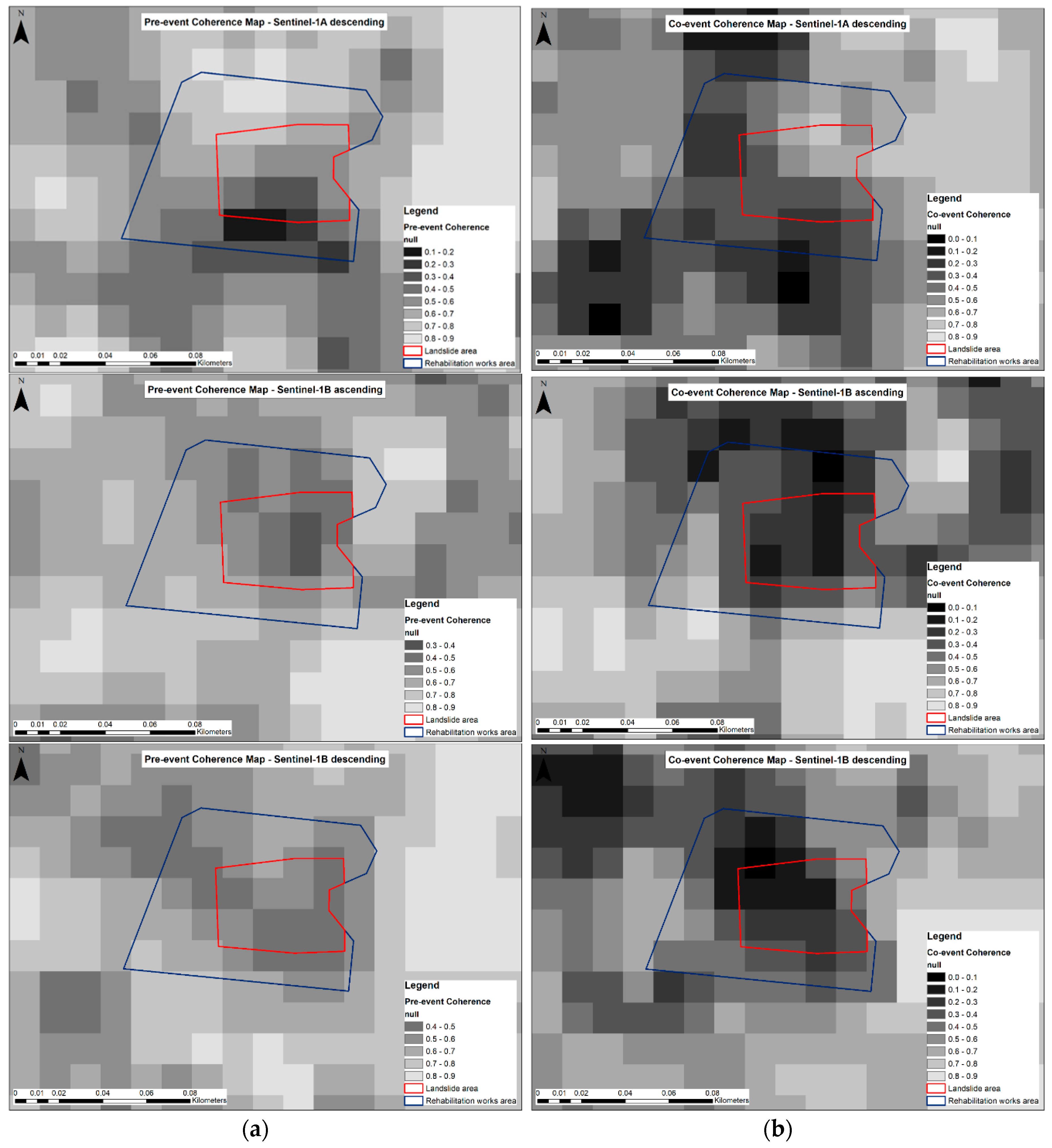
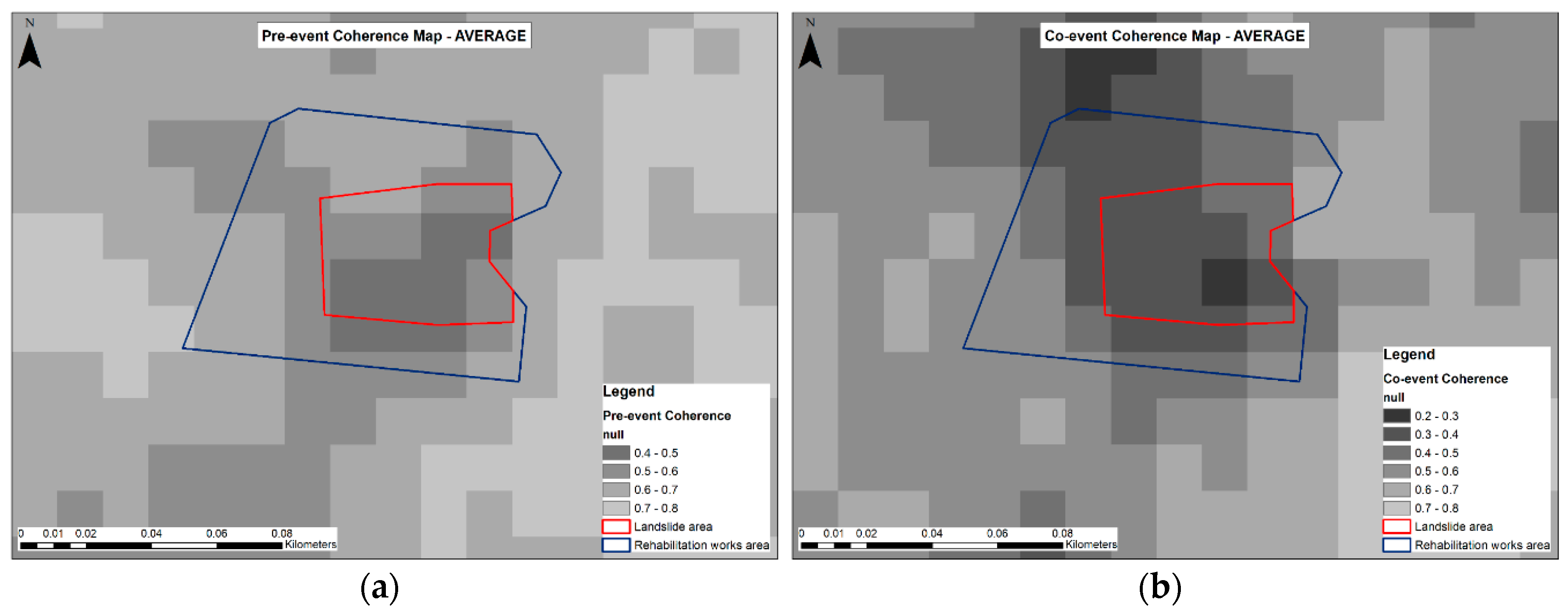
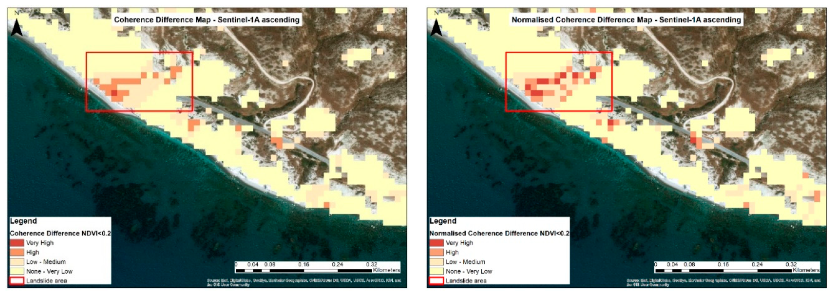
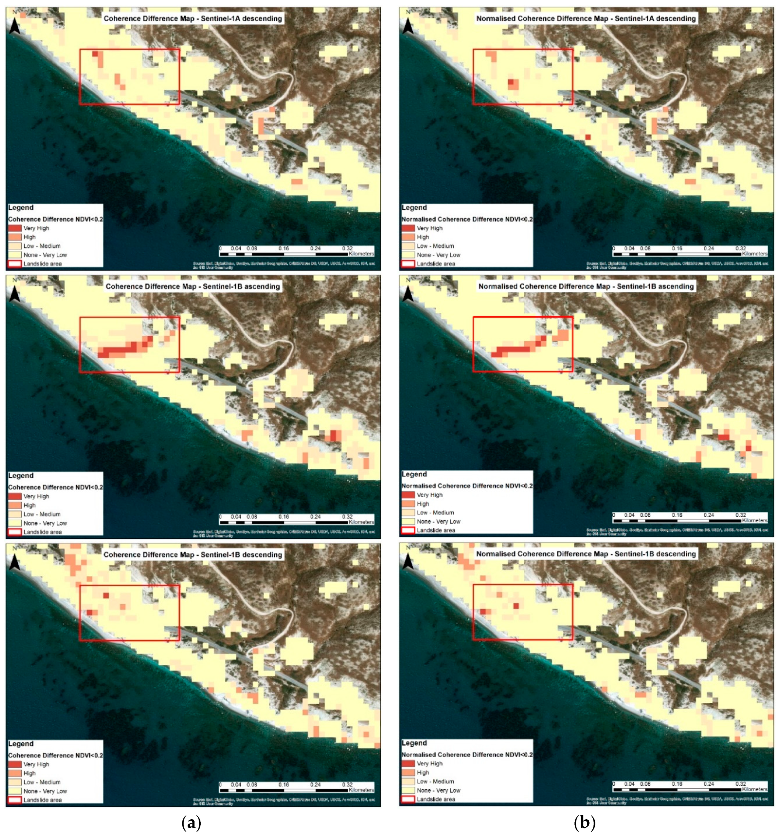
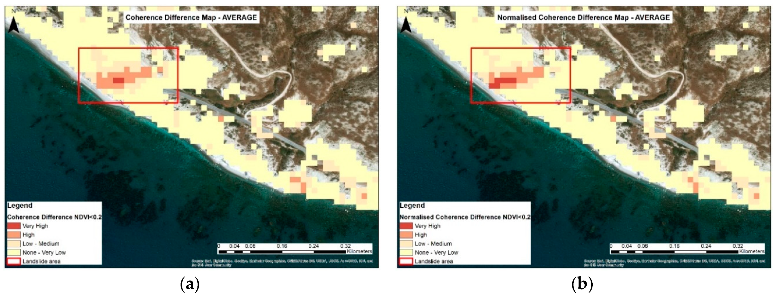
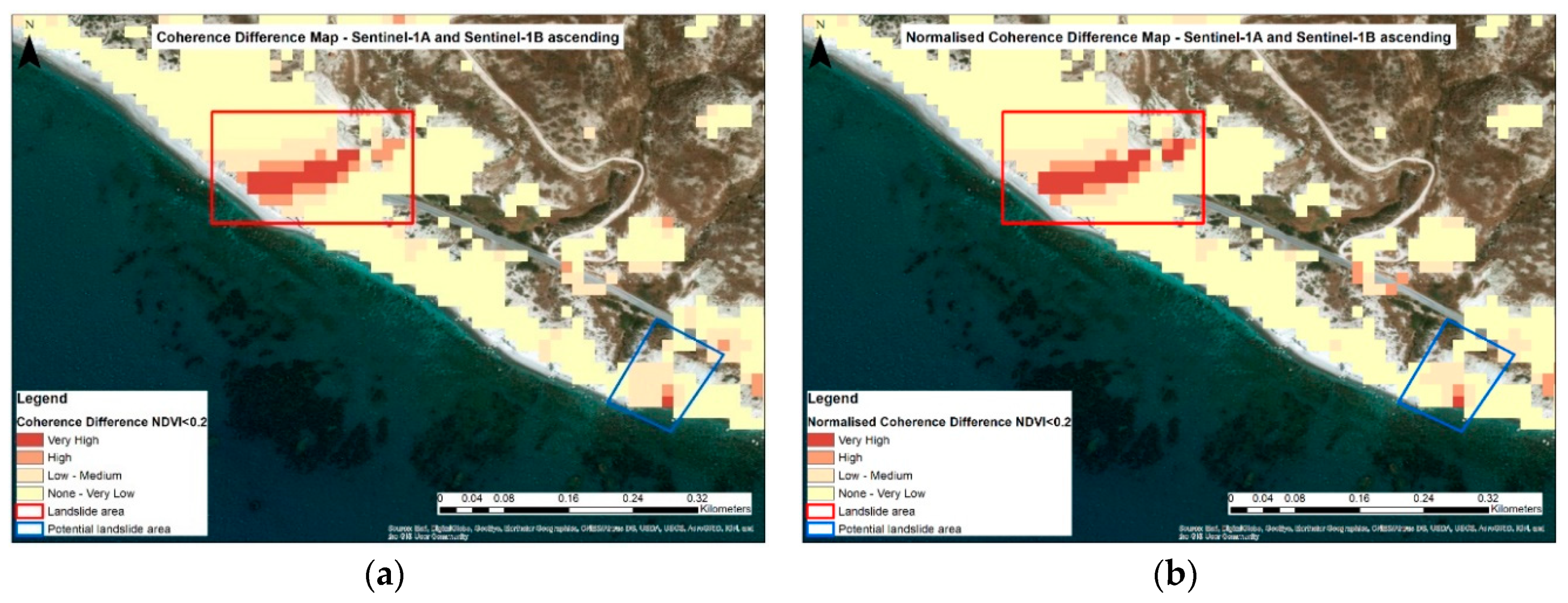
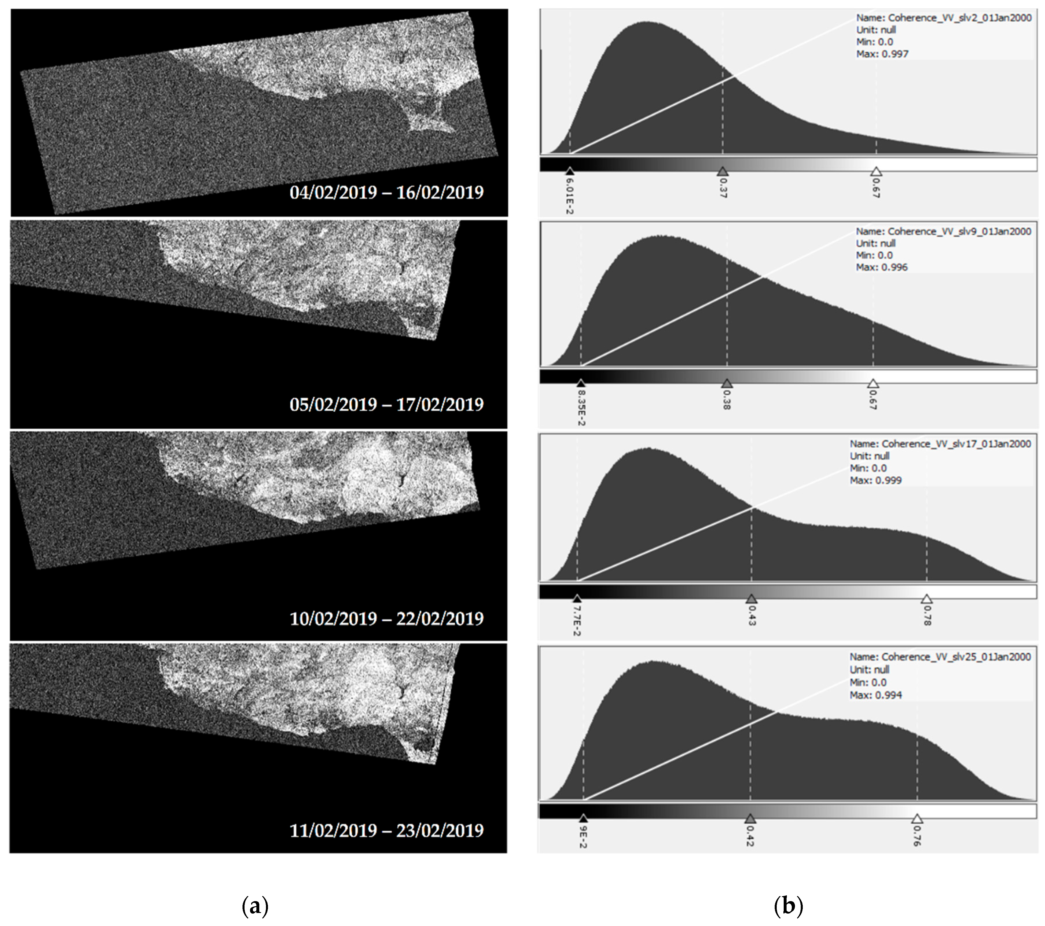
4.2. Coherent Change Detection Analysis—Landslide Detection
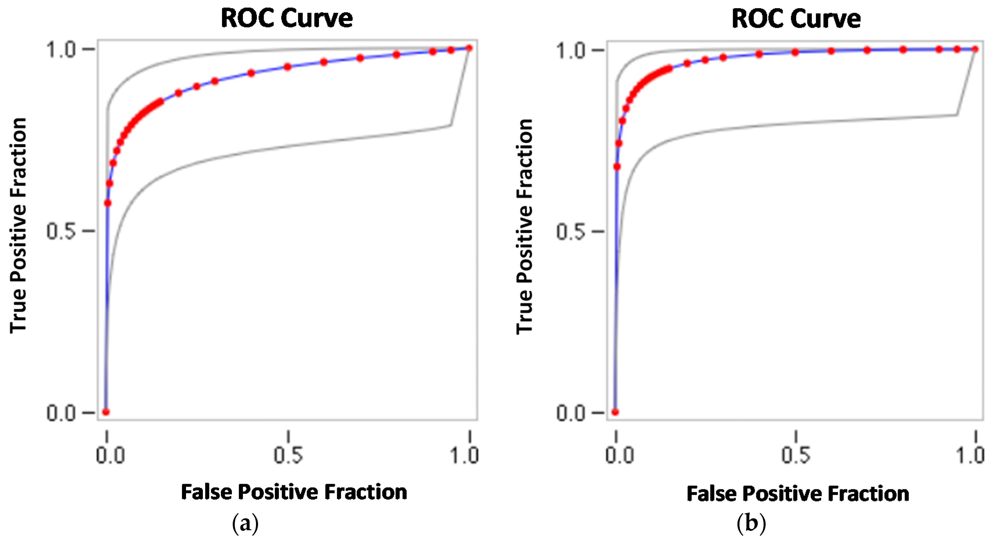
4.3. ROC Analysis
4.4. Validation of Methodology
5. Discussion
6. Conclusions
Supplementary Materials
Author Contributions
Funding
Acknowledgments
Conflicts of Interest
References
- Rodrigue, J.P.; Comtois, C.; Slack, B. The Geography of Transport Systems, 2nd ed.; Routledge Taylor & Francis: London, UK; New York, NY, USA, 2006. [Google Scholar] [CrossRef]
- Jenelius, E.; Mattsson, L.G. Road Network Vulnerability Analysis of Area-Covering Disruptions: A Grid-Based Approach with Case Study. Transp. Res. Part A Policy Pract. 2012, 46, 746–760. [Google Scholar] [CrossRef]
- Jenelius, E.; Petersen, T.; Mattsson, L.G. Importance and Exposure in Road Network Vulnerability Analysis. Transp. Res. Part A Policy Pract. 2006, 40, 537–560. [Google Scholar] [CrossRef]
- Geological Survey Department. The Seismicity of Cyprus; Press and Information Office of the Republic of Cyprus: Nicosia, Cyprus, 2012.
- Alexandris, A.; Griva, I.K.; Abarioti, M. Remediation of the Pissouri Landslide in Cyprus. Int. J. Geoengin. Case Hist. 2016, 4, 14–28. [Google Scholar] [CrossRef]
- Geological Survey Department. Landslides in Cyprus and Their Consequences to Built Environment; Press and Information Office of the Republic of Cyprus: Nicosia, Cyprus, 2013.
- Geological Survey Department. Geological Survey Department|Ground Suitability. Available online: http://www.moa.gov.cy/moa/gsd/gsd.nsf/page37_en/page37_en?OpenDocument (accessed on 12 January 2020).
- Northmore, K.J.; Charalambous, M.; Hobbs, P.R.N.; Petrides, G. Engineering Geology of the Kannaviou, ’Melange’ and Mamonia Complex Formations—Phiti/Statos Area, S W Cyprus: Engineering Geology of Cohesive Soils Associated with Ophiolites, with Particular Reference to Cyprus. Report of the EGARP Research Group British Geological Survey, No. EGARP-KW 86/4; Report of the Geological Survey Department of Cyprus, No. G/EG/15. 1986. Available online: http://nora.nerc.ac.uk/id/eprint/19494/1/WNRR86004.pdf (accessed on 14 May 2019).
- Northmore, K.J.; Charalambous, M.; Hobbs, P.R.N.; Petrides, G. Complex Landslides in the Kannaviou, Melange, and Mamonia Formations of South-West Cyprus. In 5th International Symposium on Landslides; Bonnard, C., Ed.; Balkema Publishers: Brookfield, WI, USA, 1988; pp. 263–268. [Google Scholar]
- Pantazis, T.M. Landslides in Cyprus. Bulletin 1969, 4, 1–20. [Google Scholar]
- Charalambous, M.; Petrides, G. Contribution of Engineering Geology in the Planning and Development of Landslide Prone Rural Areas in Cyprus. In Engineering Geology and the Environment; Balkema: London, UK, 1997; pp. 1205–1210. [Google Scholar]
- Hart, A.B.; Ruse, M.E.; Hobbs, P.R.N.; Efthymiou, M.; Hadjicharalambous, K. Assessment of Landslide Susceptibility in Paphos District, Cyprus. In GRSG-AGM Geoenvironmental Remote Sensing Conference; The Geological Society of London: London, UK, 2010. [Google Scholar]
- Hart, A.B.; Hearn, G.J. Landslide Assessment for Land Use Planning and Infrastructure Management in the Paphos District of Cyprus. Bull. Eng. Geol. Environ. 2013, 72, 173–188. [Google Scholar] [CrossRef]
- Saha, A.K.; Gupta, R.P.; Arora, M.K. GIS-Based Landslide Hazard Zonation in the Bhagirathi (Ganga) Valley, Himalayas. Int. J. Remote Sens. 2002, 23, 357–369. [Google Scholar] [CrossRef]
- Lee, S.; Lee, M.-J. Detecting Landslide Location Using KOMPSAT 1 and Its Application to Landslide-Susceptibility Mapping at the Gangneung Area, Korea. Adv. Space Res. 2006, 38, 2261–2271. [Google Scholar] [CrossRef]
- Fourniadis, I.G.; Liu, J.G.; Mason, P.J. Landslide Hazard Assessment in the Three Gorges Area, China, Using ASTER Imagery: Wushan–Badong. Geomorphology 2007, 84, 126–144. [Google Scholar] [CrossRef] [Green Version]
- Park, N.-W.; Chi, K.-H. Quantitative Assessment of Landslide Susceptibility Using High-resolution Remote Sensing Data and a Generalized Additive Model. Int. J. Remote Sens. 2008, 29, 247–264. [Google Scholar] [CrossRef]
- Pradhan, B. Remote Sensing and GIS-Based Landslide Hazard Analysis and Cross-Validation Using Multivariate Logistic Regression Model on Three Test Areas in Malaysia. Adv. Space Res. 2010, 45, 1244–1256. [Google Scholar] [CrossRef]
- Bhattacharya, A.; Arora, M.K.; Sharma, M.L.; Vöge, M.; Bhasin, R. Surface Displacement Estimation Using Space-Borne SAR Interferometry in a Small Portion along Himalayan Frontal Fault. Opt. Lasers Eng. 2014, 53, 164–178. [Google Scholar] [CrossRef]
- Mullissa, A.G.; Tolpekin, V.; Stein, A.; Perissin, D. Polarimetric Differential SAR Interferometry in an Arid Natural Environment. Int. J. Appl. Earth Obs. Geoinf. 2017, 59, 9–18. [Google Scholar] [CrossRef]
- Da Lio, C.; Tosi, L. Land Subsidence in the Friuli Venezia Giulia Coastal Plain, Italy: 1992–2010 Results from SAR-Based Interferometry. Sci. Total Environ. 2018, 633, 752–764. [Google Scholar] [CrossRef] [PubMed]
- Liosis, N.; Marpu, P.R.; Pavlopoulos, K.; Ouarda, T.B.M.J. Ground Subsidence Monitoring with SAR Interferometry Techniques in the Rural Area of Al Wagan, UAE. Remote Sens. Environ. 2018, 216, 276–288. [Google Scholar] [CrossRef]
- Tzouvaras, M.; Kouhartsiouk, D.; Agapiou, A.; Danezis, C.; Hadjimitsis, D.G. The Use of Sentinel-1 Synthetic Aperture Radar (SAR) Images and Open-Source Software for Cultural Heritage: An Example from Paphos Area in Cyprus for Mapping Landscape Changes after a 5.6 Magnitude Earthquake. Remote Sens. 2019, 11, 1766. [Google Scholar] [CrossRef] [Green Version]
- Morishita, Y.; Lazecky, M.; Wright, T.J.; Weiss, J.R.; Elliott, J.R.; Hooper, A. LiCSBAS: An Open-Source InSAR Time Series Analysis Package Integrated with the LiCSAR Automated Sentinel-1 InSAR Processor. Remote Sens. 2020, 12, 424. [Google Scholar] [CrossRef] [Green Version]
- Di Martire, D.; Tessitore, S.; Brancato, D.; Ciminelli, M.G.; Costabile, S.; Costantini, M.; Graziano, G.V.; Minati, F.; Ramondini, M.; Calcaterra, D. Landslide Detection Integrated System (LaDIS) Based on in-Situ and Satellite SAR Interferometry Measurements. Catena 2016, 137, 406–421. [Google Scholar] [CrossRef]
- Bovenga, F.; Pasquariello, G.; Pellicani, R.; Refice, A.; Spilotro, G. Landslide Monitoring for Risk Mitigation by Using Corner Reflector and Satellite SAR Interferometry: The Large Landslide of Carlantino (Italy). Catena 2017, 151, 49–62. [Google Scholar] [CrossRef]
- Strozzi, T.; Klimeš, J.; Frey, H.; Caduff, R.; Huggel, C.; Wegmüller, U.; Rapre, A.C. Satellite SAR Interferometry for the Improved Assessment of the State of Activity of Landslides: A Case Study from the Cordilleras of Peru. Remote Sens. Environ. 2018, 217, 111–125. [Google Scholar] [CrossRef] [Green Version]
- Pieraccini, M.; Mecatti, D.; Noferini, L.; Luzi, G.; Franchioni, G.; Atzeni, C. SAR Interferometry for Detecting the Effects of Earthquakes on Buildings. NDT E Int. 2002, 35, 615–625. [Google Scholar] [CrossRef]
- Lin-lin, G.; Cheng, E.; Polonska, D.; Rizos, C.; Collins, C.; Smith, C. Earthquake Monitoring in Australia Using Satellite Radar Interferometry. Wuhan Univ. J. Nat. Sci. 2003, 8, 649–658. [Google Scholar] [CrossRef]
- Dong, Y.; Li, Q.; Dou, A.; Wang, X. Extracting Damages Caused by the 2008 Ms 8.0 Wenchuan Earthquake from SAR Remote Sensing Data. J. Asian Earth Sci. 2011, 40, 907–914. [Google Scholar] [CrossRef]
- Pritchard, M.E.; Simons, M. A Satellite Geodetic Survey of Large-Scale Deformation of Volcanic Centres in the Central Andes. Nature 2002, 418, 167–171. [Google Scholar] [CrossRef] [PubMed]
- Pavez, A.; Remy, D.; Bonvalot, S.; Diament, M.; Gabalda, G.; Froger, J.-L.; Julien, P.; Legrand, D.; Moisset, D. Insight into Ground Deformations at Lascar Volcano (Chile) from SAR Interferometry, Photogrammetry and GPS Data: Implications on Volcano Dynamics and Future Space Monitoring. Remote Sens. Environ. 2006, 100, 307–320. [Google Scholar] [CrossRef] [Green Version]
- Meyer, F.J.; McAlpin, D.B.; Gong, W.; Ajadi, O.A.; Arko, S.; Webley, P.W.; Dehn, J. Integrating SAR and Derived Products into Operational Volcano Monitoring and Decision Support Systems. ISPRS J. Photogramm. Remote Sens. 2015, 100, 106–117. [Google Scholar] [CrossRef]
- Schaefer, L.N.; Di Traglia, F.; Chaussard, E.; Lu, Z.; Nolesini, T.; Casagli, N. Monitoring Volcano Slope Instability with Synthetic Aperture Radar: A Review and New Data from Pacaya (Guatemala) and Stromboli (Italy) Volcanoes. Earth Sci. Rev. 2019, 192, 236–257. [Google Scholar] [CrossRef]
- Bitelli, G.; Bonsignore, F.; Carbognin, L.; Ferretti, A.; Strozzi, T.; Teatini, P.; Tosi, L.; Vittuari, L. Radar Interferometry-Based Mapping of the Present Land Subsidence along the Low-Lying Northern Adriatic Coast of Italy. In Proceedings of the EISOLS 2010, Queretaro, Mexico, 17–22 October 2010; pp. 279–286. [Google Scholar]
- Hsieh, C.S.; Shih, T.Y.; Hu, J.C.; Tung, H.; Huang, M.H.; Angelier, J. Using Differential SAR Interferometry to Map Land Subsidence: A Case Study in the Pingtung Plain of SW Taiwan. Nat. Hazards 2011, 58, 1311–1332. [Google Scholar] [CrossRef]
- D’Aranno, P.; Di Benedetto, A.; Fiani, M.; Marsella, M. Remote sensing technologies for linear infrastructure monitoring. ISPRS Int. Arch. Photogramm. Remote Sens. Spat. Inf. Sci. 2019, XLII-2/W11, 461–468. [Google Scholar] [CrossRef] [Green Version]
- Closson, D.; Milisavljevic, N. InSAR Coherence and Intensity Changes Detection. In Mine Action—The Research Experience of the Royal Military Academy of Belgium; InTech: London, UK, 2017; p. 23. [Google Scholar] [CrossRef] [Green Version]
- Rocca, F.; Prati, C.; Guarnieri, A.M.; Ferretti, A. Sar Interferometry and Its Applications. Surv. Geophys. 2000, 21, 159–176. [Google Scholar] [CrossRef]
- Rosen, P.A.; Hensley, S.; Joughin, I.R.; Li, F.K.; Madsen, S.N.; Rodriguez, E.; Goldstein, R.M. Synthetic Aperture Radar Interferometry. Proc. IEEE 2000, 88, 333–382. [Google Scholar] [CrossRef]
- Zebker, H.A.; Villasenor, J. Decorrelation in Interferometric Radar Echoes. IEEE Trans. Geosci. Remote Sens. 1992, 30, 950–959. [Google Scholar] [CrossRef] [Green Version]
- Burrows, K.; Walters, R.J.; Milledge, D.; Spaans, K.; Densmore, A.L. A New Method for Large-Scale Landslide Classification from Satellite Radar. Remote Sens. 2019, 11, 237. [Google Scholar] [CrossRef] [Green Version]
- Lu, C.-H.; Ni, C.-F.; Chang, C.-P.; Yen, J.-Y.; Chuang, R. Coherence Difference Analysis of Sentinel-1 SAR Interferogram to Identify Earthquake-Induced Disasters in Urban Areas. Remote Sens. 2018, 10, 1318. [Google Scholar] [CrossRef] [Green Version]
- Abdelfattah, R.; Nicolas, J.M. Interferometric Synthetic Aperture Radar Coherence Histogram Analysis for Land Cover Classification. In Proceedings of the 2006 2nd International Conference on Information & Communication Technologies, Damascus, Syria, 24–28 April 2006; Volume 1, pp. 343–348. [Google Scholar] [CrossRef]
- Parihar, N.; Das, A.; Rathore, V.S.; Nathawat, M.S.; Mohan, S. Analysis of L-Band SAR Backscatter and Coherence for Delineation of Land-Use/Land-Cover. Int. J. Remote Sens. 2014, 35, 6781–6798. [Google Scholar] [CrossRef]
- Khalil, R.Z. InSAR Coherence-Based Land Cover Classification of Okara, Pakistan. Egypt. J. Remote Sens. Space Sci. 2018, 21, S23–S28. [Google Scholar] [CrossRef]
- Pan, Z.; Hu, Y.; Wang, G. Detection of Short-Term Urban Land Use Changes by Combining SAR Time Series Images and Spectral Angle Mapping. Front. Earth Sci. 2019, 13, 495–509. [Google Scholar] [CrossRef]
- Yun, H.W.; Kim, J.R.; Choi, Y.S.; Lin, S.Y. Analyses of Time Series InSAR Signatures for Land Cover Classification: Case Studies over Dense Forestry Areas with L-Band SAR Images. Sensors 2019, 19, 2830. [Google Scholar] [CrossRef] [Green Version]
- Erten, E.; Lopez-Sanchez, J.M.; Yuzugullu, O.; Hajnsek, I. Retrieval of Agricultural Crop Height from Space: A Comparison of SAR Techniques. Remote Sens. Environ. 2016, 187, 130–144. [Google Scholar] [CrossRef] [Green Version]
- Tamm, T.; Zalite, K.; Voormansik, K.; Talgre, L. Relating Sentinel-1 Interferometric Coherence to Mowing Events on Grasslands. Remote Sens. 2016, 8, 802. [Google Scholar] [CrossRef] [Green Version]
- Liu, C.; Chen, Z.; Shao, Y.; Chen, J.; Hasi, T.; Pan, H. Research Advances of SAR Remote Sensing for Agriculture Applications: A Review. J. Integr. Agric. 2019, 18, 506–525. [Google Scholar] [CrossRef] [Green Version]
- Suga, Y.; Takeuchi, S. Application of JERS-1 InSAR for Monitoring Deforestation of Tropical Rain Forest. Int. Geosci. Remote Sens. Symp. 2000, 1, 432–434. [Google Scholar] [CrossRef]
- Canisius, F.; Brisco, B.; Murnaghan, K.; Van Der Kooij, M.; Keizer, E. SAR Backscatter and InSAR Coherence for Monitoring Wetland Extent, Flood Pulse and Vegetation: A Study of the Amazon Lowland. Remote Sens. 2019, 11, 720. [Google Scholar] [CrossRef] [Green Version]
- Durieux, A.M.; Calef, M.T.; Arko, S.; Chartrand, R.; Kontgis, C.; Keisler, R.; Warren, M.S. Monitoring Forest Disturbance Using Change Detection on Synthetic Aperture Radar Imagery. In Applications of Machine Learning; Zelinski, M.E., Taha, T.M., Howe, J., Awwal, A.A., Iftekharuddin, K.M., Eds.; SPIE: San Diego, CA, USA, 2019; p. 39. [Google Scholar] [CrossRef]
- Ban, Y.; Zhang, P.; Nascetti, A.; Bevington, A.R.; Wulder, M.A. Near Real-Time Wildfire Progression Monitoring with Sentinel-1 SAR Time Series and Deep Learning. Sci. Rep. 2020, 10, 1322. [Google Scholar] [CrossRef] [PubMed] [Green Version]
- Hirschmugl, M.; Deutscher, J.; Sobe, C.; Bouvet, A.; Mermoz, S.; Schardt, M. Use of SAR and Optical Time Series for Tropical Forest Disturbance Mapping. Remote Sens. 2020, 12, 727. [Google Scholar] [CrossRef] [Green Version]
- Monti-Guarnieri, A.V.; Brovelli, M.A.; Manzoni, M.; Mariotti d’Alessandro, M.; Molinari, M.E.; Oxoli, D. Coherent Change Detection for Multipass SAR. IEEE Trans. Geosci. Remote Sens. 2018, 56, 6811–6822. [Google Scholar] [CrossRef]
- Uemoto, J.; Moriyama, T.; Nadai, A.; Kojima, S.; Umehara, T. Landslide Detection Based on Height and Amplitude Differences Using Pre- and Post-Event Airborne X-Band SAR Data. Nat. Hazards 2019, 95, 485–503. [Google Scholar] [CrossRef] [Green Version]
- Jung, J.; Yun, S.-H. Evaluation of Coherent and Incoherent Landslide Detection Methods Based on Synthetic Aperture Radar for Rapid Response: A Case Study for the 2018 Hokkaido Landslides. Remote Sens. 2020, 12, 265. [Google Scholar] [CrossRef] [Green Version]
- Bouaraba, A.; Acheroy, M.; Closson, D. Coherent Change Detection Performance Using High-Resolution SAR Images. Int. J. Eng. Res. Technol. 2013, 2, 3160–3166. [Google Scholar]
- Bouaraba, A.; Milisavljević, N.; Acheroy, M.; Closson, D. Change Detection and Classification Using High Resolution SAR Interferometry. In Land Applications of Radar Remote Sensing; InTech: London, UK, 2014. [Google Scholar] [CrossRef] [Green Version]
- Veci, L. Sentinel-1 Toolbox—TOPS Interferometry Tutorial; European Space Agency; Array Systems Computing Inc.: Toronto, ON, Canada, 2016. [Google Scholar]
- Braun, A.; Veci, L. Sentinel-1 Toolbox—TOPS Interferometry Tutorial; European Space Agency; SkyWatch Space Applications Inc.: Waterloo, ON, Canada, 2020. [Google Scholar]
- Plank, S.; Twele, A.; Martinis, S. Landslide Mapping in Vegetated Areas Using Change Detection Based on Optical and Polarimetric SAR Data. Remote Sens. 2016, 8, 307. [Google Scholar] [CrossRef] [Green Version]
- Watanabe, M.; Thapa, R.B.; Ohsumi, T.; Fujiwara, H.; Yonezawa, C.; Tomii, N.; Suzuki, S. Detection of Damaged Urban Areas Using Interferometric SAR Coherence Change with PALSAR-2. Earth Planets Space 2016, 68, 131. [Google Scholar] [CrossRef] [Green Version]
- Cyprus Tourism Organisation. Petra Tou Romiou (The Rock of the Greek). Nicosia, Cyprus; pp. 1–7. Available online: https://www.visitcyprus.com/files/audio_guides/written_form/Petra_tou_Romiou_afigisi_en.pdf (accessed on 14 May 2019).
- Stow, D.A.V.; Braakenburg, N.E.; Xenophontos, C. The Pissouri Basin Fan-Delta Complex, Southwestern Cyprus. Sediment. Geol. 1995, 98, 245–262. [Google Scholar] [CrossRef]
- ESA. Open Access Hub. Available online: https://scihub.copernicus.eu/ (accessed on 28 June 2019).
- ESA. SNAP|STEP. Available online: https://step.esa.int/main/toolboxes/snap/ (accessed on 17 July 2019).
- Sentinel Hub. NDVI (Normalized Difference Vegetation Index)|Sentinel Hub. Available online: https://www.sentinel-hub.com/eoproducts/ndvi-normalized-difference-vegetation-index (accessed on 9 March 2020).
- Beguería, S. Validation and Evaluation of Predictive Models in Hazard Assessment and Risk Management. Nat. Hazards 2006, 37, 315–329. [Google Scholar] [CrossRef] [Green Version]
- Eng, J. ROC Analysis: Web-Based Calculator for ROC Curves. Available online: http://www.rad.jhmi.edu/jeng/javarad/roc/JROCFITi.html (accessed on 18 March 2020).


| No. | Platform | Date (Master) | Date (Slave) | Pass Direction | Temp. Baseline | Perp. Baseline | Modelled Coherence |
|---|---|---|---|---|---|---|---|
| 1 | Sentinel-1A | 11/01/2019 | 23/01/2019 | Ascending | 12 days | 16.36 m | 0.98 |
| 2 | Sentinel-1A | 12/01/2019 | 24/01/2019 | Descending | 12 days | 108.39 m | 0.90 |
| 3 | Sentinel-1B | 17/01/2019 | 29/01/2019 | Ascending | 12 days | 43.40 m | 0.95 |
| 4 | Sentinel-1B | 18/01/2019 | 30/01/2019 | Descending | 12 days | 34.79 m | 0.96 |
| 5 | Sentinel-1A | 23/01/2019 | 04/02/2019 | Ascending | 12 days | 155.91 m | 0.86 |
| 6 | Sentinel-1A | 24/01/2019 | 05/02/2019 | Descending | 12 days | 79.26 m | 0.92 |
| 7 | Sentinel-1B | 29/01/2019 | 10/02/2019 | Ascending | 12 days | 23.22 m | 0.97 |
| 8 | Sentinel-1B | 30/01/2019 | 11/02/2019 | Descending | 12 days | 46.48 m | 0.95 |
| 9 | Sentinel-1A | 04/02/2019 | 16/02/2019 | Ascending | 12 days | 102.44 m | 0.90 |
| 10 | Sentinel-1A | 05/02/2019 | 17/02/2019 | Descending | 12 days | 12.46 m | 0.98 |
| 11 | Sentinel-1B | 10/02/2019 | 22/02/2019 | Ascending | 12 days | 17.44 m | 0.97 |
| 12 | Sentinel-1B | 11/02/2019 | 23/02/2019 | Descending | 12 days | 86.63 m | 0.92 |
| 13 | Sentinel-1A | 16/02/2019 | 28/02/2019 | Ascending | 12 days | 84.72 m | 0.92 |
| 14 | Sentinel-1A | 17/02/2019 | 01/03/2019 | Descending | 12 days | 14.88 m | 0.97 |
| 15 | Sentinel-1B | 22/02/2019 | 06/03/2019 | Ascending | 12 days | 63.25 m | 0.94 |
| 16 | Sentinel-1B | 23/02/2019 | 07/03/2019 | Descending | 12 days | 10.12 m | 0.98 |
| 17 | Sentinel-1A | 28/02/2019 | 12/03/2019 | Ascending | 12 days | 3.15 m | 0.99 |
| 18 | Sentinel-1A | 01/03/2019 | 13/03/2019 | Descending | 12 days | 87.86 m | 0.92 |
| 19 | Sentinel-1B | 06/03/2019 | 18/03/2019 | Ascending | 12 days | 30.08 m | 0.96 |
| 20 | Sentinel-1B | 07/03/2019 | 19/03/2019 | Descending | 12 days | 75.78 m | 0.93 |
| 21 | Sentinel-1A | 12/03/2019 | 24/03/2019 | Ascending | 12 days | 17.67 m | 0.97 |
| 22 | Sentinel-1A | 13/03/2019 | 25/03/2019 | Descending | 12 days | 63.94 m | 0.93 |
| 23 | Sentinel-1B | 18/03/2019 | 30/03/2019 | Ascending | 12 days | 82.29 m | 0.92 |
| 24 | Sentinel-1B | 19/03/2019 | 31/03/2019 | Descending | 12 days | 9.54 m | 0.98 |
| 25 | Sentinel-1A | 24/03/2019 | 05/04/2019 | Ascending | 12 days | 51.98 m | 0.94 |
| 26 | Sentinel-1A | 25/03/2019 | 06/04/2019 | Descending | 12 days | 57.14 m | 0.94 |
| 27 | Sentinel-1B | 30/03/2019 | 11/04/2019 | Ascending | 12 days | 30.86 m | 0.96 |
| 28 | Sentinel-1B | 31/03/2019 | 12/04/2019 | Descending | 12 days | 24.92 m | 0.97 |
| Coherence Difference | Normalized Coherence Difference | |
|---|---|---|
| Number of cases | 115 | 115 |
| Number correct | 107 | 109 |
| Accuracy | 93% | 94.8% |
| Sensitivity | 63.2% | 73.7% |
| Specificity | 99% | 99% |
| Positive cases missed | 7 | 5 |
| Negative cases missed | 1 | 1 |
| Fitted ROC area | 0.922 | 0.972 |
| Empirical ROC area | 0.897 | 0.952 |
© 2020 by the authors. Licensee MDPI, Basel, Switzerland. This article is an open access article distributed under the terms and conditions of the Creative Commons Attribution (CC BY) license (http://creativecommons.org/licenses/by/4.0/).
Share and Cite
Tzouvaras, M.; Danezis, C.; Hadjimitsis, D.G. Small Scale Landslide Detection Using Sentinel-1 Interferometric SAR Coherence. Remote Sens. 2020, 12, 1560. https://doi.org/10.3390/rs12101560
Tzouvaras M, Danezis C, Hadjimitsis DG. Small Scale Landslide Detection Using Sentinel-1 Interferometric SAR Coherence. Remote Sensing. 2020; 12(10):1560. https://doi.org/10.3390/rs12101560
Chicago/Turabian StyleTzouvaras, Marios, Chris Danezis, and Diofantos G. Hadjimitsis. 2020. "Small Scale Landslide Detection Using Sentinel-1 Interferometric SAR Coherence" Remote Sensing 12, no. 10: 1560. https://doi.org/10.3390/rs12101560
APA StyleTzouvaras, M., Danezis, C., & Hadjimitsis, D. G. (2020). Small Scale Landslide Detection Using Sentinel-1 Interferometric SAR Coherence. Remote Sensing, 12(10), 1560. https://doi.org/10.3390/rs12101560