Article

Predicting Near-Future Built-Settlement Expansion Using Relative Changes in Small Area Populations

by
Jeremiah J. Nieves
1,*,
Maksym Bondarenko
1,
Alessandro Sorichetta
1,
Jessica E. Steele
1,
David Kerr
1,
Alessandra Carioli
1,
Forrest R. Stevens
1,2,
Andrea E. Gaughan
1,2 and
Andrew J. Tatem
1
1
WorldPop, School of Geography and Environmental Science, University of Southampton, Southampton, SO17 1BJ, UK
2
Department of Geography and Geosciences, University of Louisville, Louisville, KY 40222, USA
*
Author to whom correspondence should be addressed.
Remote Sens. 2020, 12(10), 1545; https://doi.org/10.3390/rs12101545
Submission received: 17 March 2020 / Revised: 27 April 2020 / Accepted: 11 May 2020 / Published: 12 May 2020

Abstract

:
Advances in the availability of multi-temporal, remote sensing-derived global built-/human-settlements datasets can now provide globally consistent definitions of “human-settlement” at unprecedented spatial fineness. Yet, these data only provide a time-series of past extents and urban growth/expansion models have not had parallel advances at high-spatial resolution. Here our goal was to present a globally applicable predictive modelling framework, as informed by a short, preceding time-series of built-settlement extents, capable of producing annual, near-future built-settlement extents. To do so, we integrated a random forest, dasymetric redistribution, and autoregressive temporal models with open and globally available subnational data, estimates of built-settlement population, and environmental covariates. Using this approach, we trained the model on a 11 year time-series (2000–2010) of European Space Agency (ESA) Climate Change Initiative (CCI) Land Cover “Urban Areas” class and predicted annual, 100m resolution, binary settlement extents five years beyond the last observations (2011–2015) within varying environmental, urban morphological, and data quality contexts. We found that our model framework performed consistently across all sampled countries and, when compared to time-specific imagery, demonstrated the capacity to capture human-settlement missed by the input time-series and the withheld validation settlement extents. When comparing manually delineated building footprints of small settlements to the modelled extents, we saw that the modelling framework had a 12 percent increase in accuracy compared to withheld validation settlement extents. However, how this framework performs when using different input definitions of “urban” or settlement remains unknown. While this model framework is predictive and not explanatory in nature, it shows that globally available “off-the-shelf” datasets and relative changes in subnational population can be sufficient for accurate prediction of future settlement expansion. Further, this framework shows promise for predicting near-future settlement extents and provides a foundation for forecasts further into the future.

1. Introduction

In 2018, 55 percent of the world’s population lived in urbanized areas, but this is projected to increase to 68 percent by 2050, due to natural population growth, continued rural to urban migration, and the conversion of rural to urban land [1,2,3]. Most of this anticipated urban growth will be in low- and middle-income countries, specifically in small to medium sized settlements, where the majority of urban populations reside [1,4]. Logically, this growth, in conjunction with climate change, presents questions regarding sustainable development. Answers to these questions are dependent upon better understanding past and current urbanization trends to better predict future trends, minimize potential adverse outcomes and environmental impact, and maximize the benefits that can come from urbanization [1,4,5,6]. Accordingly, there is a continued need for globally comparable and standardized urban environment datasets and projections [4,6,7]. Particularly as internationally coordinated and global efforts for sustainable development, such as under the Sustainable Development Goals [8], are undertaken. The provision of these data needs to be transparent, sustainable, comparable across space and time, and available to all while being able to cope with the many definitions of urban, e.g. administrative-based, Remote Sensing (RS)-based, or population-based definitions [8,9,10].
While detailed and regular data on urban areas often exists within high-income countries, middle- and lower-income countries often lack these data, use country specific definitions of urban, or have data that is not easily accessible. Often, practitioners turn to RS-based global data that has consistently extracted urban areas and features using a definition based upon the observable human, built land cover. Recent advances have produced globally consistent urban feature datasets, which maintain relatively high spatial resolution/fidelity (<= 100m) while capturing smaller/less-dense/more-fragmented settlements [11,12,13,14,15]. Specifically, the availability of urban feature datasets globally capturing areas of Built-Settlement (BS), above ground structures that can support human habitation and or related economic processes [12,16,17], have become more common, e.g. [12,13,14,15,18,19,20]. However, these datasets still have limited temporal resolution, i.e. single time observation or cross-sectional with many years between observations. Increased temporal coverage is desirable, but sacrificing spatial resolution to do so is problematic as most human settlements, particularly those in low- to middle-income countries, are relatively smaller and less densely developed [1,21,22,23]. Compounding this is the typical time lag between global image acquisitions and the resulting dataset of built-settlement or, more generally, urban features and the associated processing costs. Further, some datasets are only produced once or cease updating with additional observations in time, leaving users of the data without continued support for a dataset-specific definition of urban. Hereafter, we refer to the general concept of “urban” as such, and use the “built-environment” to refer to all areas characterized by the presence of anthropogenic features, and use “urban features” to refer to objects within the built-environment, e.g. roads, buildings, parks. Specifically, the scenario of needing to project built-settlement extent data past last observations would logically propose extrapolative modeling as a solution.
To this regard, it is worth highlighting that the majority of the literature and existing models for projections of urban and built-environment growth focus on North America, Europe, and China, with many being city/area/regionally specific [24]. Furthermore, many of the existing continental- and global-extent urban future growth models are solely meant for exploring potential future scenarios as opposed to projecting near future urban growth grounded upon local contemporary and past observed dynamics [25,26,27]. Other models are produced from city- or country-level samples, datasets with substantial definitional or spatial/temporal disagreement, or utilize arbitrary thresholds without validation for determining non-urban-to-urban area conversion [3,28,29,30,31] Of these, many are not driven by subnational variations to determine larger scale dynamics of urban growth and transition distributions, e.g. they are statistically "global" models. Some models do not output explicit spatial extents, e.g. country-level totals of projected urban area, limiting their utility [3]. Together, these issues combined indicate a need for methods to produce a flexible and robust method of generating spatially explicit regular time series of predicted future urban environment expansion across the globe.
Our goal was to leverage developments in statistical methods, data availability, and computing resources to create a globally applicable urban expansion modelling framework to project beyond the last observations while addressing the above existing needs. Using observed time-series of BS extents and coincident small area population changes we were able to produce spatially explicit annual BS extent maps representing projected near-future BS expansion for multiple points in time. Here we introduce such a modelling framework and validate its performance against withheld time-specific past RS-derived observations and time-specific manual delineations of BS.

2. Materials and Methods

2.1. Study Areas and Data

To test across a variety of BS morphologies, environmental contexts, and developmental contexts, in addition to countries with varying spatial details of the input census-based population data, we sample countries less present in previous spatial urban and BS modelling studies [24], including Switzerland, Panama, Uganda, and Vietnam (Table 1). Additionally, these countries were chosen to capture a variety of population magnitudes, densities, and distributions across space as well as socio-economic, urban morphological, topographical, and data quality (e.g. spatial fineness of subnational population data) contexts. Given that this extrapolative framework builds off the previously fit interpolative Built-Settlement Growth Model (BSGMi) [16], the same set of covariates were used as in [16] for either predicting transition probability in the random forest (Table 2, superscript “c”) or in the remainder of the disaggregative process. These covariates were selected based upon previous literature to give immediate environmental context and information regarding settlement connectivity and proximity [28,32,33], e.g. negative relationship between slope and likelihood of transition, positive relationship between likelihood of transition and distance to existing BS. Covariates were time specific or assumed to be temporally invariant (Table 2), and were pre-processed and appropriately resampled to 3 arc seconds (~ 100m at the Equator) as detailed in Lloyd et al. [34].

2.1.1. Built-Settlement Data

Our chosen representation of BS was the “Urban” class, number 190, of the annual European Space Agency Climate Change Initiative thematic land cover dataset (https://www.esa-landcover-cci.org/; hereafter, ESA). We selected the ESA RS-derived extents data for its annual coverage, at the time of the study, from 1992 to 2015. It has recently been extended to provide coverage for the years 2016–2018 [46]. While ESA RS-derived extents have moderate spatial resolution, 10 arc sec resolution (~ 300m at Equator), its annual temporal resolution allows for the withholding of years for validation. In our period of interest, 2000 to 2015, the ESA data begins with a Medium Resolution Imaging Spectrometer (MERIS) imagery derived baseline land cover map and detects thematic class changes from this map using 30 arc second (~ 1 km at the Equator) SPOT VGT imagery (1999–2013) and PROBA-V imagery (2014–2015) [47]. Any detected changes observed over two or more years are delineated at 30 arc second resolution, if prior to 2004, and, beginning with 2004, are further delineated at 10 arc second resolution using the higher resolution MERIS or PROBA-V imagery [47]. Specific to the “Urban” class, ESA incorporates the Global Human Settlement Layer (GHSL) [12,18] and Global Urban Footprint (GUF) [13] datasets to better define the class and integrate elements of two BS datasets within the overall thematic built-environment context. Initial validation efforts estimate the 2015 “Urban” class user and producer accuracies between 86–88 percent and 51–60 percent, respectively, but no information on the other years currently exist [47].
While ESA utilizes the term “urban”, it is more correctly capturing aspects of the built environment. Given the integration of the GHSL and GUF data sets, which capture built-settlement, into the ESA “urban” class, we have reason to believe that the ESA “urban” class is more correctly operating on a functional definition of “built-settlement” or “built-settlement”-like, and refer to it as such. For a more detailed discussion on built-settlement and remote-sensing representations, readers are referred to Nieves et al. (2020).

2.1.2. Population Data

Annual subnational unit area (hereafter simply “unit,”) population estimates, for 2000 through 2020, were based upon the Gridded Population of the World version 4 (GPWv4) input data [40] were produced by the Center for International Earth Science Information Network (CIESIN) and spatially harmonized as described in Lloyd et al. [34]. To clarify, we are not using the gridded GPW product, which has uniform population density within a given unit, but we are using the same tabular population count data and the associated unit areas. These counts are based upon censuses/official estimates, interpolated at the subnational level per [40] to obtain annual estimates. Each unit possesses a unique ID, referencing a globally consistent grid (3 arc seconds), with the unit areas having globally harmonized coastlines and international borders. It is worth noting that the population count data utilized here are not adjusted to the U.N. country total population estimates, which are used to account for potential biases and errors. Further, the two primary sources of uncertainty in this dataset are linked to the census figures/official estimates and the simple regression used to obtain the annual estimates with few assumptions.

2.1.3. OpenStreetMap Data

OpenStreetMap (OSM) is an open database of user-contributed, edited, and curated spatial data also known as. While OSM offers global extent, like other Volunteered Geographic Information (VGI) [48], its completeness varies across space, with particular gaps in low and middle income countries, and has data quality that can vary both within and between countries [49,50]. Contrastingly, in the best of cases, OSM can approach the quality of official datasets [51]. However, agreed upon means of assessing VGI data quality and accuracy varies and is still debated [52]. Nonetheless, OSM data are used to fill data gaps where official/commercial datasets do not exist or are not publicly accessible and have improved or produced useful analyses and derived datasets, (e.g. [13,34,53,54,55,56,57]).
For validation, we utilized the OSM building footprints around the municipalities of Visp, Brig-Glis, Naters, and Ried-Brig, Switzerland, where agreement between modelled extents and RS-derived extents were particularly large. The mountainous 119 km2 area (rectangular bounds: 7.8606508° 46.2779033°; 8.0224478°, 46.3298123°) had a 2015 combined mid-year population of approximately 32,430 [58]. It contained 8,083 buildings manually delineated by OSM contributors, of which we contributed over an additional 1,700 buildings in an effort to have near 100 percent coverage of permanent vertical structures covered by the definition of BS. We inspected all building footprints in the area for accuracy and temporal coincidence with true colour imagery in 2015. The resource intensive nature of manually delineating and checking building footprints precluded us from carrying out more widespread validations of this nature during this study. The building footprints are provided in the linked data repository (https://data.mendeley.com/datasets/cm6bnzvzfj/1).

2.2. Built-Settlement Growth Model extrapolation (BSGMe)

2.2.1. Overview

Here we take annual time-series of BS extents spanning 2000–2010 and estimated annual changes in BS population and unit-average BS population density changes to predict short-term (within five years) BS extents from 2011 through 2015. BS population is the population coincident with the BS extents and unit-average BS population density is the BS population of a unit divided by the BS area within the same unit. We refer to the set of years making each time series as TS where TS = {2000, 2001, …,2010} and, expanding the notation from Nieves et al. [16], the first and last years of the input time series are referred to as t0 and t1, respectively. We test this extrapolative Built-Settlement Growth Model (BSGMe) framework using an annual time series of RS-based ESA BS extents from 2000–2010 (TSESA).
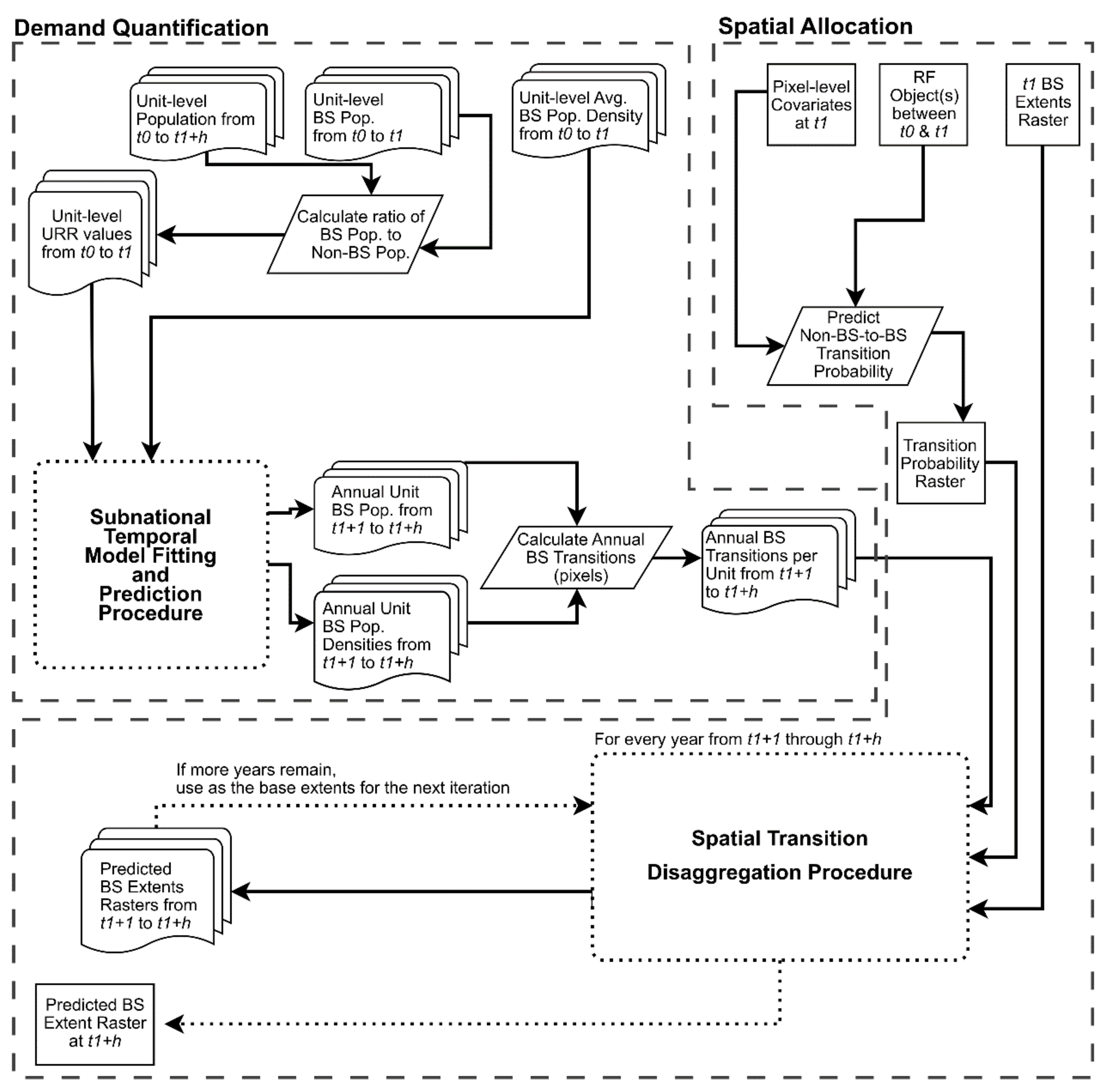
Similar to the BSGMi framework [16], the BSGMe framework has two primary components of “Demand Quantification” and “Spatial Allocation”, shown here in Figure 1.
We generalize the BSGMe framework with following steps:
  • Create gridded population maps for each year in the input TS, following Stevens et al. [54].
  • For all years in the TS, extract the unit-specific population sum that is coincident with the year’s corresponding BS extents and derive the unit-average BS population density
  • Independently for each unit, and using a rolling origin validation, select the single best fitting model for BS population and, separately, unit-average BS population density from three classes of models:
    • Auto-Regressive Integrated Moving Average (ARIMA),
    • Error, Trend, Seasonality (ETS), and
    • Generalized Linear Model (GLM) given log-transformed inputs.
  • For each unit, use the final selected model for BS population and for unit-average BS population density to predict short-term annual BS population and annual unit-average BS population density starting with year t1+1 and ending with year t1+h, where in this case 1 ≤ h ≤ 5 and represents the projection horizon, in numbers of years.
  • Use these estimates to derive the unit-specific annual quantity demand of non-BS-to-BS transitions by dividing the BS population by the BS population density.
  • Create a transition probability surface using a Random Forest (RF) based upon the observed transitions between t0 and t1 of the input time-series and covariates corresponding to t0.
  • Take the fit relationships between the occurrence of transitions and the predictive covariates, contained in the final RF model, and predict the future non-BS-to-BS transition probability surface using the same covariates, but corresponding to year t1, as the input.
  • For each unit and iteratively for all years t1+1 through t1+h, spatially disaggregate the predicted annual unit-level transitions (steps 1–5) using the base transition probability surface (steps 5–6) and, if available, unit-relative weights derived from changes in lights-at-night brightness, similar to Nieves et al. [16].
These steps produce annual binary spatial predictions of BS extent in gridded format. All modelling and analyses were carried out using R 3.4.2 [59] and utilized the IRIDIS 4 high-performance computing cluster. All code is provided in the linked data repository (https://data.mendeley.com/datasets/cm6bnzvzfj/1). Full process diagrams are provided in Appendix A, Figure A1 and Figure A2.

2.2.2. Demand Quantification

Built-Settlement Population Estimation

To obtain a set of annual estimated population surfaces for our study areas, we used the method detailed by Stevens et al. [54] to dasymetrically disaggregate [60,61] the census-based population from the unit-level to 3 arc second (~100m at the Equator) pixels. We independently modelled each country and year utilizing time-specific and, assumed, time-invariant predictive covariates (see Appendix A, Table A1). We included the distance-to-nearest BS edge at the year 2000 and the distance-to-nearest BS edge for the given year as predictive covariates. This corresponded with our assumption that population relates to inner parts of BS agglomerations differently from the outer parts and to avoid exaggerated areas of low population density relative to previously modelled years [16,62]. Annually, for each unit, we extracted and summed the populations from pixels that were within year-specific BS extents and derived the annual unit-average BS population density. This resulted in annual time-series of BS population estimates and unit-average BS population densities for every unit in the study area, covering eleven years.

Time-Series Model Fitting and Built-Settlement Population Projections

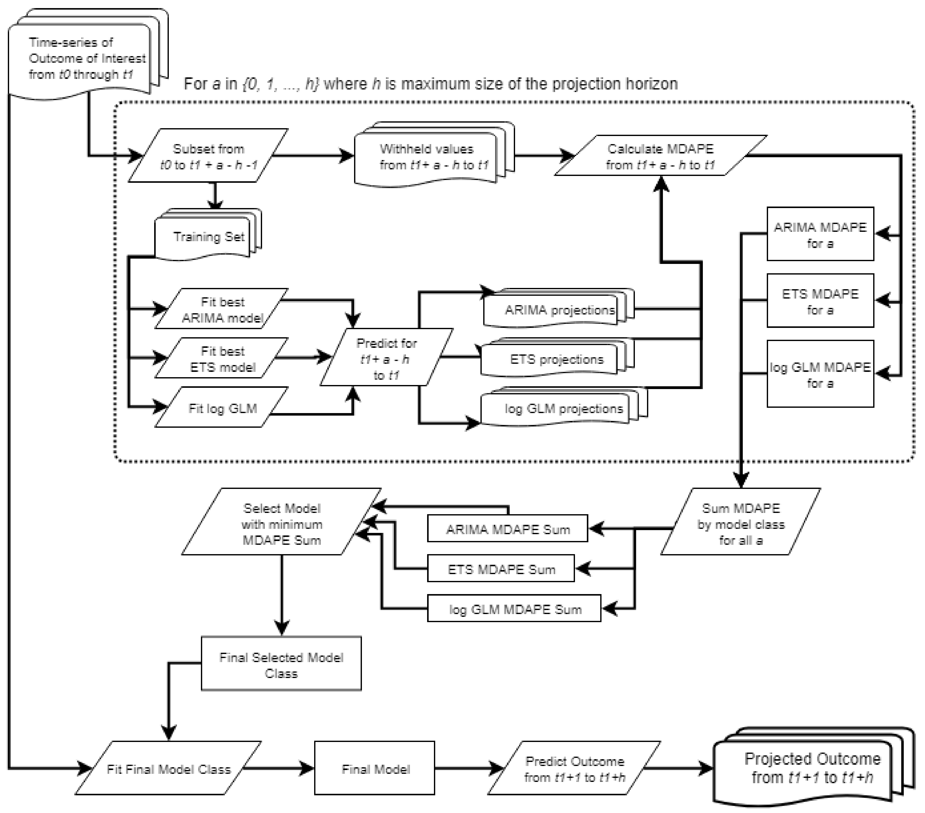
Using these annual unit-level time-series, we predicted future unit BS population and unit-average BS population density using a single model fitting and selection process detailed in Figure 1. For each unit, this process fits three classes of models: ARIMA models, ETS models, and an identity-link GLM model with log-transformed input values, all using a rolling origin framework validation in the final, i.e. between-class, model selection process.
ARIMA models [63,64,65] and ETS models [64,65,66,67] are two autoregressive model classes often applied to time-series data, including population forecasts [68]. Both classes have dependent model terms based upon preceding values in the input time-series. ETS models are based upon the assumption of non-stationary, i.e. the mean and variance of the underlying process are not constant, and can approximate non-linear processes [64]. Conversely, ARIMA models assume stationarity and a linear correlation between the values of the time-series, but remain a standard in forecasting time-series [64,69]. The best model within the ARIMA class relies on an automated fitting procedure utilizing unit root tests, iterative step-wise parameter fitting, and the resultant lowest Akaike Information Criterion (AIC) value, as described in detail by Hydman and Khandakar [64]. ETS class models are selected in an automated fashion, as described in Hyndman et al. [65], utilizing maximum likelihood parameter estimation, the corrected AIC (AICc), and bootstrapping simulation. For the ARIMA and ETS model classes only the number of years since year t0 and temporally preceding values in the input time-series were available as predictive covariates.
Generalized Linear Models (GLMs) provide a single consistent framework for linking the linear-based systematic elements of regression-type models, associated with Normal, binomial, Poisson, gamma, and other statistical distributions, with their respective random components through an integrated fitting procedure based upon maximum likelihood [70]. Here, we utilized an identity link function, and provided log-transformed input data with the number of years since year t0 as the sole predictive covariate.
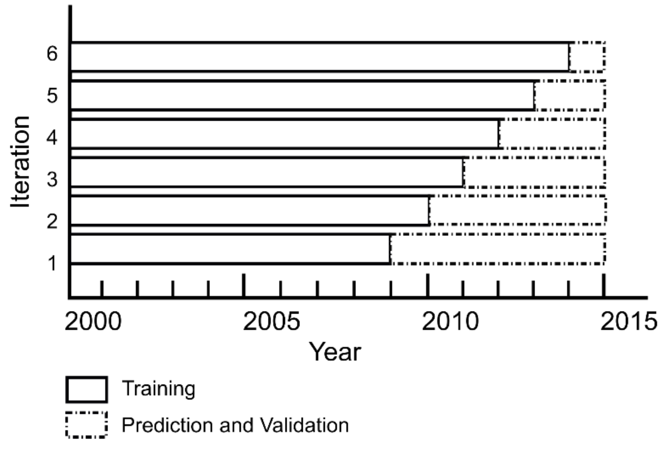
During the fitting of these model classes we utilized a rolling origin validation (Figure 2) of each model class in anticipation of needing to determine the final model based upon a single metric of error across the different number of years predicted into the future. A rolling origin validation fits a selected model upon an iteratively changing sample size and an inversely changing number of future time steps, i.e. “the rolling origin” (Figure 2) [71,72,73]. We used the MeDian Absolute Percent Error (MDAPE) as our forecasting error metric as opposed to the more common Mean Absolute Percent Error (MAPE). The MAPE, compared to other metrics, has the advantage of avoiding large errors when the true value is near zero [74]. The MDAPE retains the advantages of the MAPE, but is less influenced by extreme values and is more robust than the MAPE [69,74]. It can be written as:
M D A P E = m e d i a n y ^ y   y * 100 .   )
where y ^ is the predicted outcome of interest and y is the withheld observed outcome.
Given our short input time-series (Nts = 11) and our projection horizon between one and five years (1 ≤ h ≤ 5), we utilized a maximum horizon of five years in the model fitting too. This meant the model classes were iteratively fit with between six (i.e. 2000–2005) and ten (i.e. 2000–2009) input observations, with all other observations withheld, and then predicted between one and five years, respectively, forward of the last input year of the given iteration sample. Each iteration produced a set of annual absolute percent errors for the projected years, of which the median was recorded. The sum of MDAPE values across all iterations represents the total error of each model class for the given unit. Written mathematically, for a given unit i, maximum horizon length h, and a being the index of the given set of iterations, the MDAPE sum within the rolling origin framework can be written as
MDAPE i sum = a = 0 h [ MDAPE a ] = a = 0 h [ median ( { | y ^ k y k y k * 100 | } k = n ts + h n ts + h ) ]
where the sample training series for a given iteration can be written as nts = t1 + a – h and the set of projected years within an iteration are calculated for each year k that takes on values between n t s + 1 ,   ,   n t s + h , e.g., for h = 3 and a = 3 the models are fit on years 1 to 8 with a set of predictions made for y ^ n t s + 1 ,   y ^ n t s + 2 ,   y ^ n t s + 3 . After the rolling origin framework finished, for each unit, we selected the best model between model classes based upon the lowest M D A P E i s u m and fit the selected model class on the entire available time series. Normally, using the entire time series is cause for concern of model over fitting. However, our larger concern was that excluding later observations in the extremely short time series could lead to excluding important information late in the series. Therefore, we assumed that fitting only on a subset of the time-series would be as harmful, or more so, than potentially overfitting any given unit. After the refitting, and independently for each unit, we predicted the final outcome of interest through our projection horizon, in this case 2011–2015. Full process diagram of this sub-procedure is provided in Appendix A, Figure A2.
This time-series model selection and prediction procedure was used twice in the demand quantification component of the BSGMe: once for predicting future BS population and once for predicting future unit-average BS population density (Figure 1). For predicting future BS population, we first transformed, and later back-transformed, BS population to an “BS/Non-BS Ratio” to ensure BS population never exceeded total population [1]. We then calculated the final year- and unit-specific number of projected non-BS-to-BS transitions by dividing the projected BS population by the corresponding projected BS population density.

2.2.3. Spatial Allocation

Projecting non-Built-Settlement (BS)-to-BS Transition Probabilities Surface

After calculating annual unit-level demand for non-BS-to-BS transitions, we spatially allocated transitions to the pixel level, producing annual projected BS extents. First, we trained a RF on transitions observed between 2000 and 2010 with spatially coincident covariates corresponding to the year 2000 (Table 2). This RF was created following the sampling and training procedures in Nieves et al. [16] where an iterative covariate selection procedure was employed, removing covariates that did not improve the accuracy of the RF model. In this scenario, we were assuming that relationships observed between transitions and the predictive covariates persist into the near future. Therefore, we projected forward to estimate the probability of transition surface after 2010 by using 2010 representative covariates as input covariates (Figure 1). The values of the resulting probability surface range from 0.00 to 1.00 and represent the posterior probability of a pixel being classified as transitioning between, originally 2000 and 2010, 2010 and 2015 [75]. We elected to use a RF due to its efficiency and scalability as well as its ability to model complex interactions and non-linear phenomenon using a non-parametric approach with minimal input [75]. Further, RFs have been shown in at least one study to outperform other machine learning type methods, such as support vector machines [76], and showed satisfactory performance in Nieves et al. [16].

Annually Adjusting non-BS-to-BS Transition Probabilities

While many projections are “truly future” scenarios and no earth observation data would be available, here we are validating the framework within a scenario where the “future” projection period is one where the input BS extent dataset does not have coverage, i.e. as if ESA had stopped producing the dataset at 2010, and we have access to observed lights-at-night (LAN) data during our projection period (2011–2015). With this, we follow the procedure in Nieves et al. [16] of using average annual unit-normalized lagged LAN brightness to modify the period probability produced by the RF to a more annual representation of the unit-specific probabilities of transition. The assumption behind this process is that pixels with larger unit-relative changes in annual LAN brightness correspond to a larger probability of non-BS-to-BS transition occurring at those location and vice versa. That is, if a relatively large increase, with respect to the given subnational unit, in the LAN brightness occurred between years and given that the area was not already BS, we would assume this corresponded to a higher probability of non-BS-to-BS transition having occurred.
Using these annually adjusted unit-relative probabilities, we followed the procedure in Nieves et al. [16] to spatially disaggregate the demand quantification component-derived projected annual transitions from the unit-level to the pixel-level (Figure 1). Differing from Nieves et al. [16], we did not restrict where the transitions can occur, excluding existing BS areas and bodies of water, as, being the “future”, we did not know observed transition locations in the projection period. This iterative disaggregation began with the last observed extents in year t1 (2010) and, within each unit i, if we had n number of predicted transitions for our given projected year, we selected pixels in unit i with the nth highest annually adjusted probabilities, and transitioned them from non-BS-to-BS. This is in line with Nieves et al. [16], Tayyebi et al. [77], Linard et al. [28] and others where it is assumed that pixels with higher transition probabilities are more likely to transition than pixels with lower probabilities. We repeated this process for all years in the projection period, using the previously projected year as the prior BS extents to expand upon, and output the union of the prior extents and the new projected transition as the next year’s BS extents (Figure 1). All resulting and derived data are provided in the linked data repository (https://data.mendeley.com/datasets/cm6bnzvzfj/1).

2.3. Analysis

Validation and Comparison Metrics

We validated BSGMe projected extents against the withheld ESA extents for 2011, 2012, 2013, 2014, and 2015. The ESA data themselves are an imperfect reference, but our goal was to replicate the pattern of ESA’s capture of BS relative to BS population and BS population density changes. Therefore, “True” in all of these validations represents agreement of the BSGMe projections with the temporally corresponding withheld ESA validation extents and “False,” equally, represents disagreement. For every year, we classified every pixel in the study areas as either True Positive, False Positive, False Negative, or True Negative, TP, FP, FN, TN, respectively. Using these pixel-level designations, we calculated classification contingency-table metrics, listed in Table 3, at the unit-level.
The fact that most BS land cover and non-BS land cover is in agreement from any time A to near future time B is simply due to the fact that most land cover remains the same, i.e. persistence, causes issues when looking at classification metrics [79]. Some methods exist for accounting for this [79], but because our input datasets assume that “once BS, always BS”, we cannot utilize these adjustments in our binary classification assessment. Hence, the best alternative is to compare all results to a null or naïve model [79]. We utilized a conservative naïve model where we assumed that the 2010 BS extents remained constant through 2015, i.e. lacking any other information we assumed the BS extents remain approximately the same over the short-term. In end user applications, when missing year-specific BS extents, the last available BS extents are commonly used as a substitute. We validated the 2010 extents following the same procedures to compare to the modelled extents.
We also visually compared the 2015 BSGMe modelled extents and the withheld ESA 2015 extents to 2015 true color imagery, available via Google Earth [80], to better understand areas of over/under prediction. We further carried out a quantitative classification validation of the 2015 BSGMe modelled extents and the withheld ESA RS-derived 2015 extents against the presence of OSM building footprints in Switzerland around the municipalities of Visp, Brig-Glis, Naters, and Ried-Brig, where relative model over prediction appeared to be exceptionally bad.

3. Results

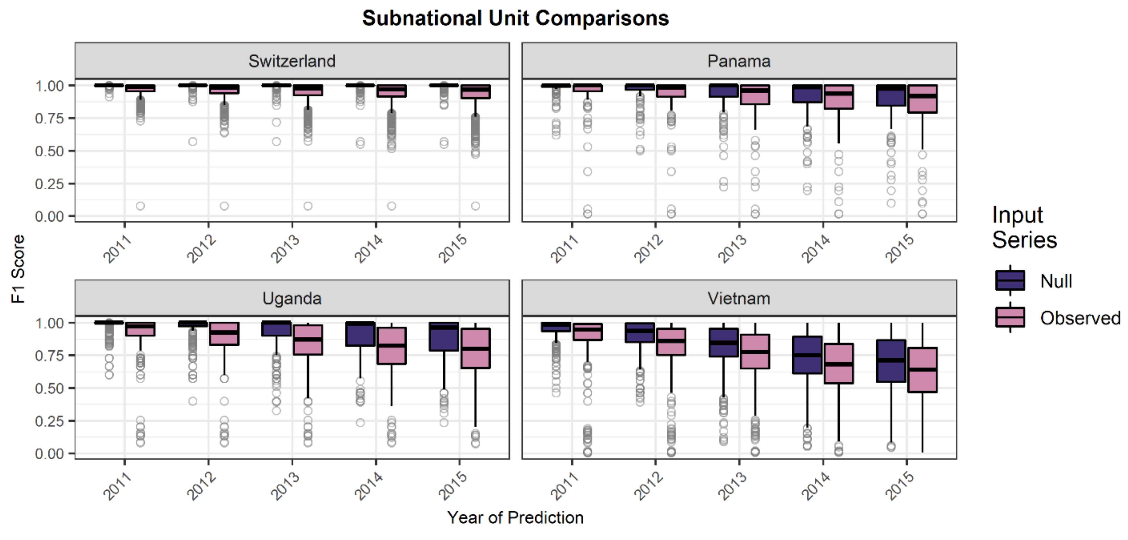
Looking at the distribution of unit-level F1 scores in Figure 3, we show that all models decrease in performance as projection horizon increases, with Vietnam having the most rapid rate of decrease and largest net decrease. In all countries, it appears that the naïve model outperforms all other models to varying degrees, but not typically by much in all countries with the exception of Uganda (Figure 3).
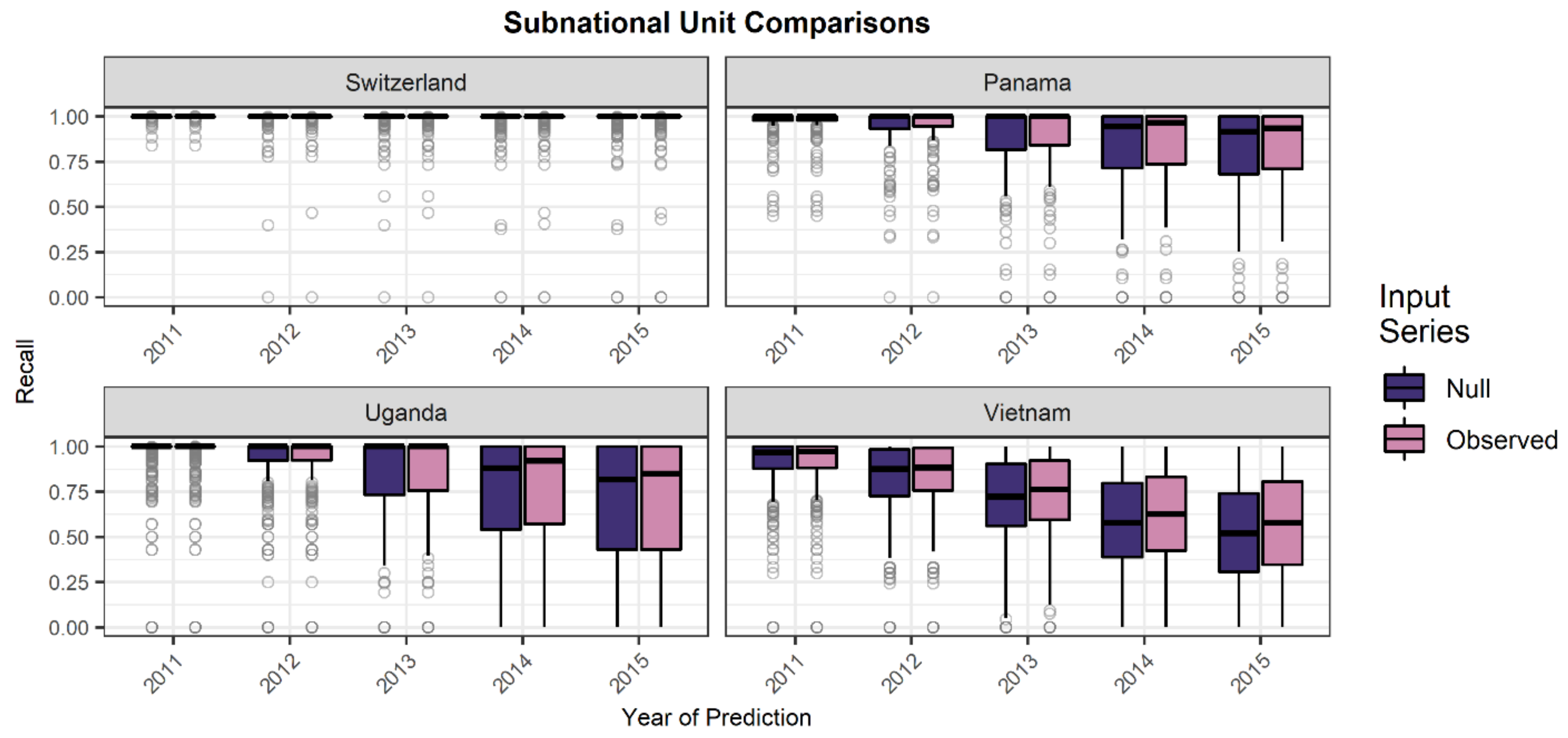
Further investigating the distributions of F1 scores, in Figure 4, we show that recall also decreases as the projection horizon increases with Vietnam again having the most rapid and largest net decrease in recall. This makes sense as, according to the ESA RS-derived extent datasets, Vietnam had the largest relative growth while Switzerland, whose recall distributions are near identical and perfect across all input series, had very little growth, i.e. recall is driven here in Switzerland largely by persistence (Figure 4, Table 1). As expected, as the projection year increases, the recall of the BSGMe produced projections outperforms the naïve model by an increasing magnitude. Unexpectedly, considering Figure 4, Uganda had relatively high values of recall, although the variance of unit-level recall was the largest of our study countries (Figure 4).
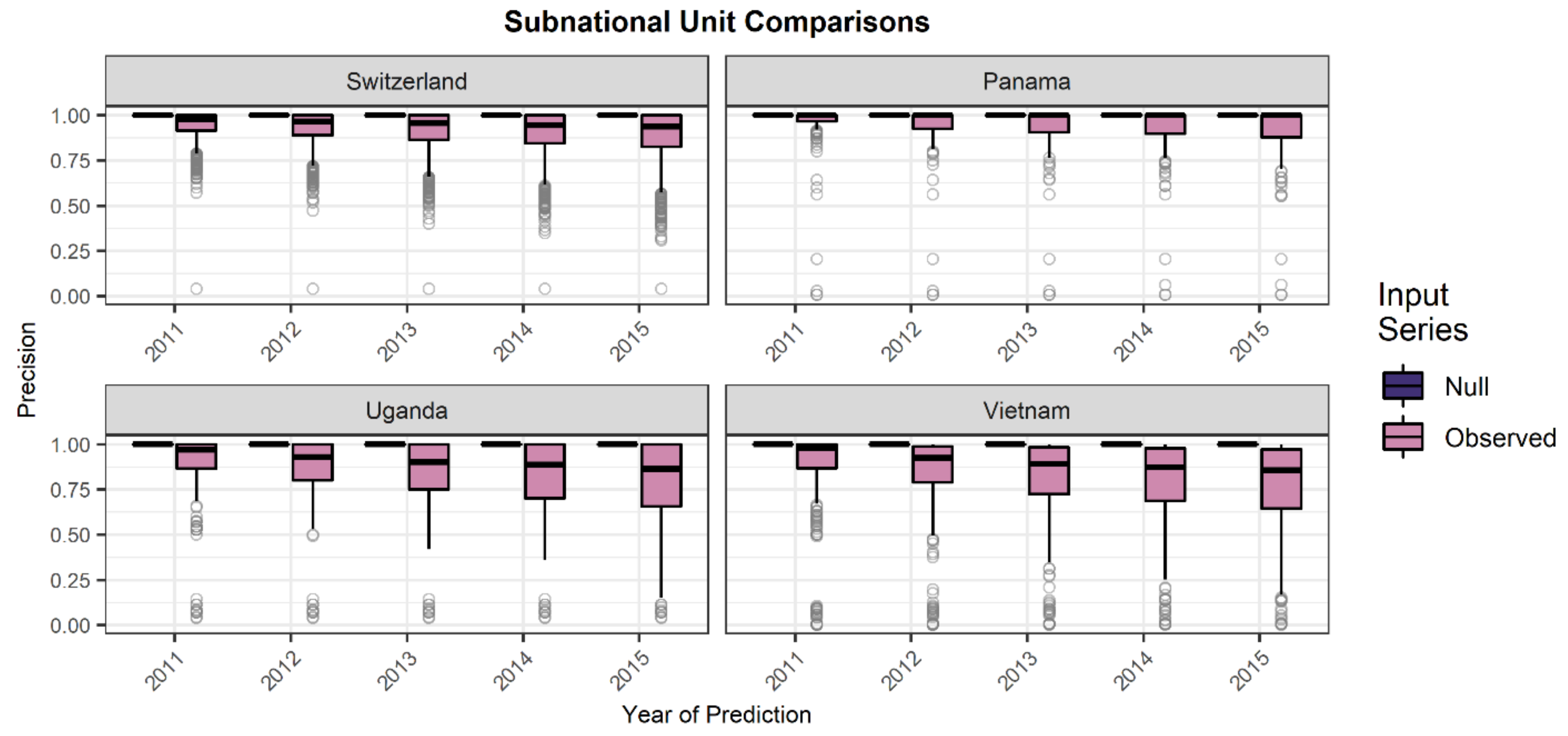
Looking at the distribution of precision values in Figure 5, precision values decrease as the projection year increases across all countries and input series, except the naïve model because false positive could not occur with the extents remaining static. The low and variable precision shown by Uganda (Figure 5) potentially explains the observed variance of its F1 scores (Figure 3). Our best guess for the low precision here was that the ESA RS-derived extents were not as good as the population data in Uganda, i.e. leading to worse demand quantification and spatial allocation in the production of the time-series and propagating error through the BSGMe projections.
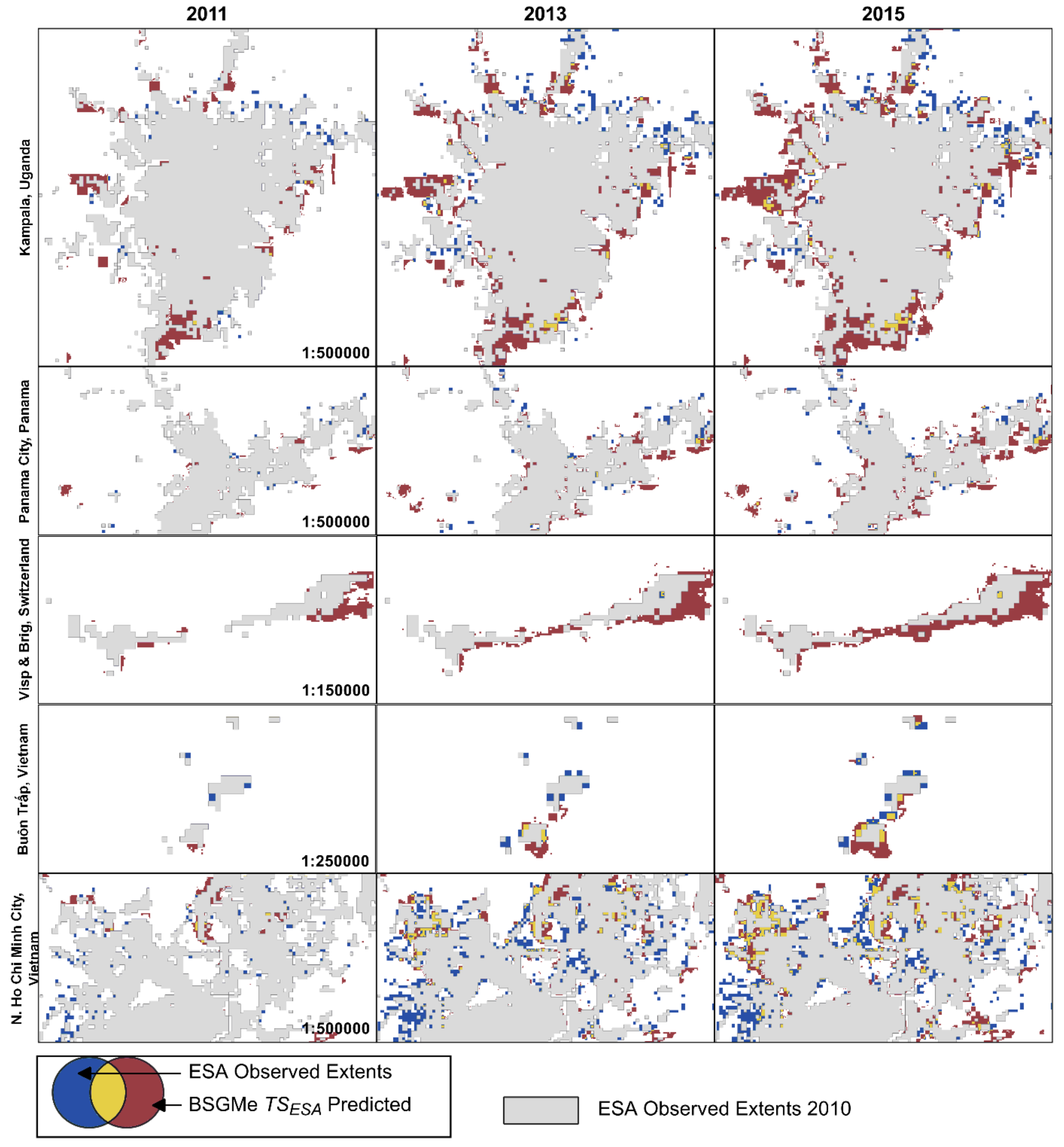
Examining the predicted and observed extents of even a subset of projection years and areas within the study countries, Figure 6, gives some context for the findings in Figure 3, Figure 4 and Figure 5. The same temporal trend of increases in “false positives”, red in Figure 6, imply large areas of over-prediction relative to areas of agreement with ESA RS-derived extents. Areas of false negatives, blue in Figure 6, when examined against time-specific true color imagery [80] seem to consistently coincide with low to mid-density areas of BS intermixed with trees.
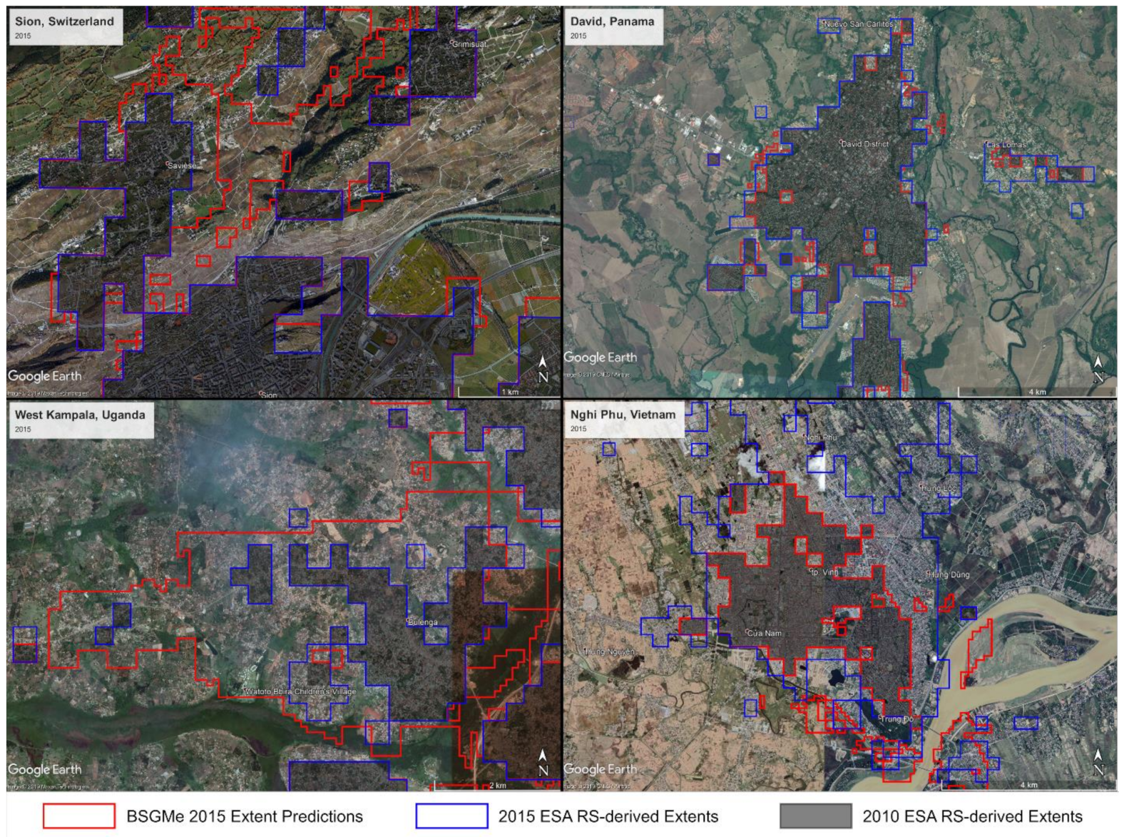
Of these examples, Kampala, Uganda appeared to have the greatest magnitude of “false positives” while the Visp and Brig area of Switzerland appeared to have the largest relative number of “false positives” to RS-based observed transitions (Figure 6). This prompted us to investigate these areas more with time specific true-color imagery [80]. Looking at time-specific true color imagery in an area of west Kampala, Uganda, we overlaid the observed (ESA) and predicted (BSGMe) extents at 2015(Figure 7). We see that all extents are missing areas of BS, with ESA RS-derived extents missing the more fragmented and less densely settled areas (Figure 7). Within the West Kampala, Uganda scene (Figure 7, bottom left), the 2015 BSGMe-derived extents appear to have large numbers of false positives relative to the 2015 ESA RS-derived extents. Interpreting the 2015 imagery in conjunction with the extents, it is apparent that the BSGMe extents are exhibiting better recall of true BS extents (Figure 7, bottom left), suggesting that perhaps the findings of Figure 3, Figure 4 and Figure 5 are conservative relative to the true BS extents. Although less dramatic, this was the generally the case in numerous other areas of Uganda and the other sampled countries (Figure 7, top left). However, there were examples (Figure 7, bottom right) where the BSGMe extents underestimated the true BS extents and where false positives did occur.
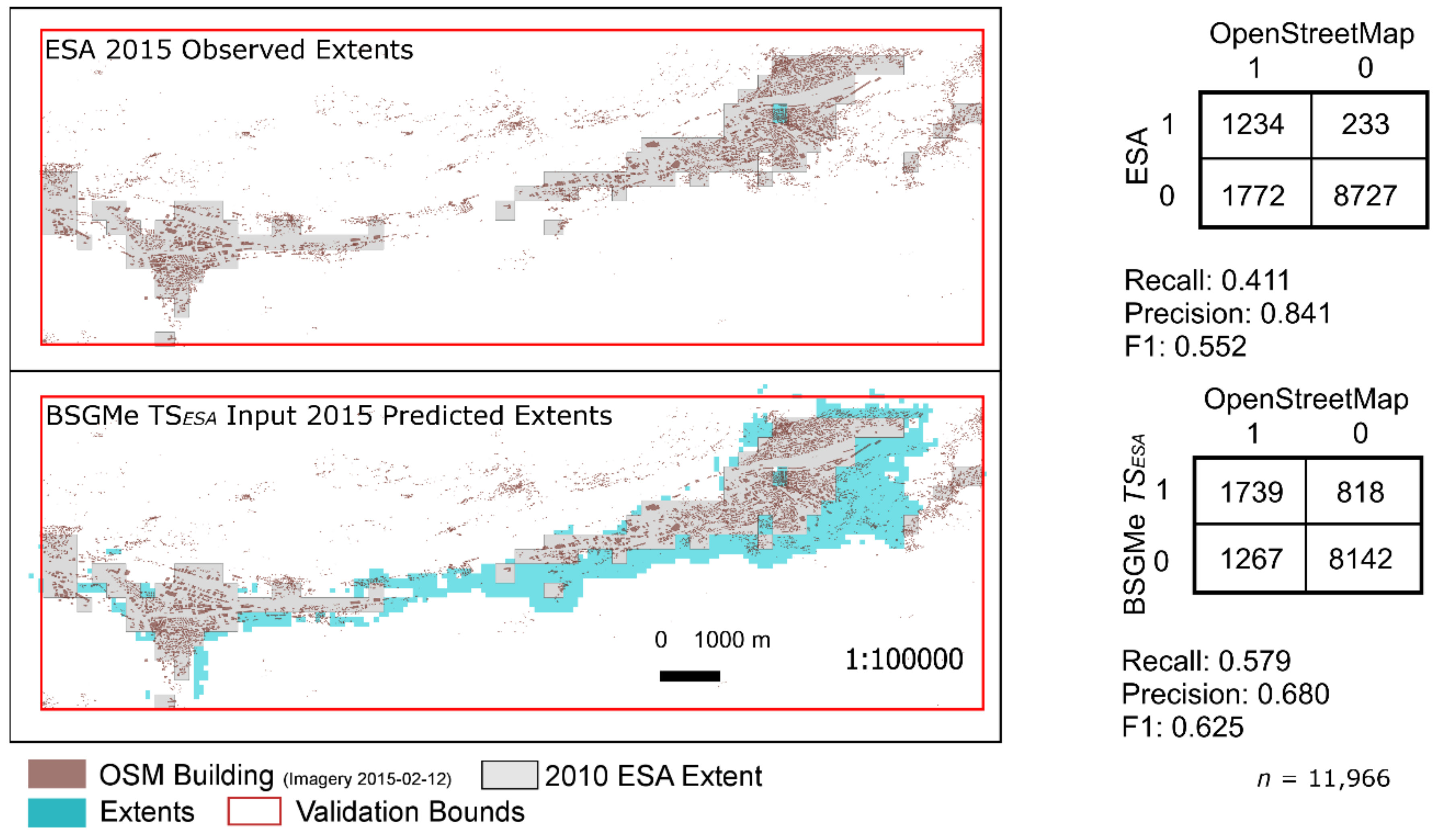
To begin to approach estimating how much this overestimation of false positives might be, we decided to compare an area of what appeared to be extreme over prediction by the2015 BSGMe extents relative to the 2015 ESA RS-derived extents, around Visp and Brig, Switzerland, and validate both by using the corresponding manually delineated building footprints (OpenStreetMap Contributers, 2019). By 2015, the ESA RS-derived data said there was 1,477 pixels of BS while the BSGMe-derived extents predicted 2,557 pixels of BS (Figure 8). When we compared these extents OSM building footprint data, corresponding to those present in 2015 and with near 100% coverage, across 11,966 3 arc-second pixels in the validation area, we showed that many of the areas are, in fact, not false positives (Figure 8). In fact, the observed ESA data only has a recall of 41.1% compared to the BSGMe performance of 57.9%, but the ESA extents do retain the highest precision of 84.1% (Figure 8). Considering both recall and precision simultaneously, we see that the BSGMe extents have a F1 score of 0.625 which represents approximately a 12% increase in F1 score to the ESA data (0.552) garnered by a 50% increase in recall, but at the expense of a 20% decrease in precision (Figure 8).

4. Discussion

We have shown that the BSGMe projects BS extents into the near future with, in many cases, large agreement with the input dataset’s withheld observations for predicted years (Figure 3, Figure 4 and Figure 5). Beyond this, we found support that the validation of the BSGMe predictions, relative to the ESA RS-based observations, could be underestimating the true accuracy (Figure 7 and Figure 8). We displayed this visually for a large proportion of Kampala, Uganda, and other example areas (Figure 7). Further, we quantified it by comparing against manually delineated building footprints for smaller settlements of the Visp and Brig area in Switzerland, showing the BSGMe having a 40 percent increase in recall and a 12 percent increase in F1 score relative to the ESA RS-based data (Figure 8).
Overall, there are inherent limits to the BSGMe approach. The framework is sensitive to the size and configuration of the subnational units used, per the Modifiable Areal Unit Problem (MAUP) [81]. We would expect that less certainty in the spatial allocation would accompany larger unit area, but the effect of unit size on demand quantification is less clear; although Nieves et al. [16] found that smaller unit size was associated with higher overall unit interpolative accuracy. Additionally, we believe that the framework would be highly sensitive to the input projected population data, yet this characteristic could have potential utility for exploring deterministic outcomes of various input urban population projection scenarios. To further clarify, while here we utilized the Stevens et al. (2015) method for producing unit level estimates of BS population, any unit-level estimates of BS population and BS population density can be provided to the BSGMe modelling framework.
Given the dasymetric nature of the BSGMe framework, measures of uncertainty that would otherwise be generated by the RF, ARIMA, ETS, and GLM models within the framework cannot be propagated to the end predicted BS extents [54,60,61,82]. This uncertainty propagation limit is similar to and was noted in the interpolative settlement modelling framework of Nieves et al. [16]. However, in general, it would be expected that the accuracy of BSGMe extrapolative predictions would have a positive relationship with any errors associated with its input datasets. For instance, if the user-selected representation of BS or estimates of BS population were relatively inaccurate, it would be logical to suppose that the framework would be tasked with sorting out noisier relationships between relative population change and BS extent expansion, and likely have poorer framework performance. In light of the framework relationships to input data error/uncertainty and the limits of propagating and quantifying this uncertainty, it is recommended that any user of this framework compare modelled outputs to the input data layers as well as the uncertainty metrics of the individual framework modelling components, which are recorded in tabular format by the framework code (see code in linked data repository https://data.mendeley.com/datasets/cm6bnzvzfj/1).
Due to persistence, the future BS projections with the highest agreement was the naïve model (Figure 3). Ignoring the actual ground truth, the model comparisons by metrics without potential end-user context are an oversimplification, with metrics like accuracy and F1 score treating a false-positive disagreement equally bad as a false-negative disagreement. It is more useful to interpret the results with a user’s defined loss function in mind [83]. Should the user want to have few disagreements of any type, then the naïve model extents would be logical. However, if the user-defined cost of missing new BS extents would be a greater loss than the alternative cost of additional false-positives, the user would likely avoid the naïve approach in favor of one of the BSGMe predicted extents. Combined with the fact the false-positives of the BSGMe validations are likely inflated (Figure 3, Figure 4, Figure 5, Figure 6, Figure 7 and Figure 8), it is likely that the difference in precision performance from that of the naïve model is smaller than presented here.
It is important to note that these validation findings are specific to the input ESA RS-derived extents data and the spatial scale of the input representation of BS (originally 10 arc second and then resampled to 3 arc seconds). More generally, the model framework presented here can accept any binary input of urban/built-environment/built-settlement. Although, given the framework’s strong reliance on relative changes in population being indicative of relative changes in urban/built-environment/built-settlement, a functional definition of urban/built-environment/built-settlement that corresponds with aspects of the built-environment more likely to be spatially coincident with populations would be most appropriate. Whether our assumptions of population being usable as a proxy for the underlying drivers of BS expansion holds at other spatial scales of BS representation, e.g. 30m Landsat-derived, 12.5m radar-derived, or 500m Moderate Resolution Imaging Spectroradiometer (MODIS)-derived, remains unclear. Supplemental findings for a city-based area, from Nieves et al. [16], observed decreased interpolative agreement when applied to a 1 arc second radar-optical dataset, rescaled to 3 arc seconds. Theoretically, we would expect individual agency, local planning conditions, micro-economic level decision-making, and other “intangibles” from a country, to a global-extent application standpoint, to have a much larger role in the siting of BS at the average individual building scale (~ 10m–30m). However, most of this type of data, if it exists, remains unavailable across large extents and across time when working in low- to middle-income contexts.
The utilization of land cover to estimate a continuous population surface, using that population surface to estimate BS population, aggregate the BS population to the unit level to then estimate non-BS-to-BS transition demand at the unit level naturally raises a concern of circular reasoning or endogeneity. From a modelling perspective, the larger more important question is, “Why is the model being developed and what questions does it attempt to address?”. Our purpose here was to develop a modelling framework capable of accurately predicting near future built-settlement expansion and to answer the question of whether this could be done by looking at subnational changes in population counts corresponding to BS areas. With this in mind, we do not believe circular reasoning, or “endogeneity”, is a significant issue for the following reasons. First, our modelling framework is not an explanatory model [84] and endogeneity is, by definition, an issue of causality. Our framework falls somewhere between predictive and descriptive in nature [85] and makes no attempts at statistical inference of causation in any of its components; even the random forest is algorithmic in nature [84,86]. We were interested in utilizing the correlations in our framework to create the best predictions possible, not to infer anything on the causal linkages. Secondly, there is precedent for using the hierarchical structure of population data in this manner; other model frameworks have used changes in population, at a spatial scales coarser than the scale of prediction, to quantify demand for urban area expansion [16,26,27,28,29,77,87], with one even using pixel level population to drive pixel level transitions [88]. Further, Angel et al. [3] also used geospatial and remotely sensed data to determine estimates of “urban” population and population densities that were subsequently aggregated and then used to predict future urban areas. However, this does raise the issue of fitness for purpose, similar to the discussion in Leyk et al. [11], where end users interested in causal questions and wishing to utilize datasets produced with certain covariates should assess how it was created to avoid the issue of endogeneity.
As expected, we observed that as the time from the last observation increased, the BSGMe projection decreased in agreement with the withheld ESA RS-derived validation extents. This positive association between time from last observation and projection agreement/accuracy is inherent to extrapolative models but could likely be reduced by using longer input time series, should data allow. While the automatic fitting procedure for ARIMA and ETS class models has been shown to have consistently good performance in the short-term (5–6 time steps) [64], this is predicated upon substantially longer time series (20 to 144 observations in the cited M3 competition series data [89]) than are typical with current BS or urban based population datasets at subnational unit level and with large or global extent. Due to the growing uncertainty that accompanies longer projections, we do not recommend extending this framework past the short-term without longer input time series and without further assessment. Another reason we do not currently recommend using the framework for longer term predictions is the lack of including other causal aspects of non-BS -to-BS transition, e.g. economic and planning/zoning information. We excluded such data from the framework because it is typically not available globally, for multiple time points, and at subnational resolutions.
We save unit- and year-specific 95% confidence intervals produced, via bootstrapping, by the ARIMA and ETS models [64], but we did not produce similar intervals for the GLM models (see linked data repository https://data.mendeley.com/datasets/cm6bnzvzfj/1). This was because we were only utilizing the GLMs to capture the general linear trend and not inferring the true value bounds, due to an inability check for the necessary corresponding inferential assumptions for every subnational unit in an automatic, efficient, and robust manner.

5. Conclusions

Here, we have shown the BSGMe model framework to be flexible and automatable across several environmental, urban morphological and input-data quality contexts while maintaining acceptable agreement with validation data and even surpassing the performance of the input dataset’s withheld observations when compared to manually interpreted conditions in time-specific true-color imagery. This framework is novel in that it is globally applicable, with no need for user or expert input parameters, and relies largely on relative changes in subnational population to determine the timing and magnitude of changes. While validated across four countries, this framework is scalable to producing global extents across different periods and with different input BS and population datasets. Proof in point, the WorldPop Programme (www.worldpop.org) adopted this modelling framework to produce global annual BS extents at 100m resolution from 2015 through 2020, using input time-series from 2000–2014 based upon observed and BSGMi interpolated extents (https://doi.org/10.5258/SOTON/WP00649) derived from Global Human Settlement Layer, ESA urban land cover class, and Global Urban Footprint [34].
Being able to produce annual datasets of near future BS extents, and the intermediate BS populations, have a variety of end user applications where investigating potential impacts of BS population changes and BS spatial expansion can have impact, such as public health, sustainability, planning and infrastructure, and transportation management. However, as seen in this study, users should utilize auxiliary data in conjunction with their expert and or local knowledge of the application/study area to assess whether the modelled extents are suitable for their applications and needs. Additionally, this framework and its open-source code can be used as a platform for further investigating deterministic relationships between population, population densities, and BS expansion. The extent predictions of the BSGMe framework can also be utilized, in a setup similar to this study, by producers of future BS and urban feature data sets to re-investigate areas of disagreement between the BSGMe and their extraction algorithm, knowing that there is a heightened probability of BS being truly present (Figure 7 and Figure 8).
As the temporal resolution of global BS and urban feature data sets catch up to their high spatial resolution, further investigations of this framework will become more accessible and feasible as well as have reduced uncertainty in their conclusions. However, as evidenced in this study, there is a continued need for an independent multi-temporal data set of urban features with global extent that can be used for training and or validation. While OSM offers global extent, it has its own biases in completeness [50,51] and, more significantly, lacks any temporal attributes. One potential solution would be for the producers of urban feature data sets to make their manually identified training and validation points, footprints, and sample grid cells publicly available, e.g. by some research collaboration akin to POPGRID Data Collaborative (www.popgrid.org) with agreed upon documentation, data attribute, and definitional standards. Until such a time, large scale ground truthing, much less temporal ground truthing, of BS or urban features will likely be limited and often surpass the resources of many studies with large or global extent.
Future work should investigate the robustness of this framework with different spatial scale representations of BS as inputs and differing lengths of input time-series. Additional experimentation with the demand forecasting methods is also a large area that remains to be explored. Further validation of more areas should also be prioritized, particularly in areas where urban feature datasets are known to have extraction issues, e.g. arid regions, in order to understand how such error may propagate through this framework into the resulting extents. Other desirable work would involve examination of the applied utility of the BS outputs produced by both the interpolative and extrapolative BSGM frameworks.

Author Contributions

Conceptualization: J.J.N., A.S., F.R.S., A.E.G., J.E.S., and A.J.T. Data Curation: J.J.N. Formal Analysis: J.J.N. Funding Acquisition: J.J.N., A.S., and A.J.T. Investigation: J.J.N. Methodology: J.J.N. and A.C. Project Administration: J.J.N. Resources: J.J.N., M.B., A.S., and A.J.T. Software: J.J.N., M.B., and D.K. Supervision: A.S., J.E.S., and A.J.T. Validation: J.J.N. Visualization: J.J.N. Writing – original draft: J.J.N. Writing – review and editing: All authors. All authors have read and agreed to the published version of the manuscript.

Funding

J.J.N. is funded through the Economic and Social Research Council’s Doctoral Training Program, specifically under the South Coast branch (ESRC SC DTP). AS is supported by funding from the Bill & Melinda Gates Foundation (OPP1134076)

Acknowledgments

Many of the spatial covariates (doi:10.5258/SOTON/WP00644) used here are the product of the “Global High Resolution Population Denominators Project” funded by the Bill and Melinda Gates Foundation (OPP1134076). The authors acknowledge the use of the IRIDIS High Performance Computing Facility, and associated support services at the University of Southampton, in the completion of this work.

Conflicts of Interest

The authors declare no conflict of interest. The funders had no role in the design of the study; in the collection, analyses, or interpretation of the data; in the writing of the manuscript, or in the decision to publish the results.

Appendix A

Figure A1. Full process diagram for the Built-Settlement Growth Model—extrapolation (BSGMe) as broken down into the “Demand Quantification” procedure and the “Spatial Allocation Procedure”. For details on the “Spatial Transition Disaggregation Procedure”, readers are referred to Nieves et al. [16]. For details on the “Subnational Temporal Model Fitting and Prediction Procedure”, readers are referred to Appendix A, Figure A2.
Remotesensing 12 01545 g0a1
Figure A2. Full process diagram of the “Subnational Temporal Model Fitting and Prediction Procedure” referenced in Appendix A, Figure A1. Readers are directed to the main text for acronym references and details on the rolling origin framework.
Remotesensing 12 01545 g0a2
Table A1. Table of time specific, or assumed temporally invariant, covariates used in the modelling of the population surfaces following the procedure from Stevens et al. [55].
CovariateTime Point(s)aOriginal SourceSource Resolution
DTE Cultivated landcover2000–2010ESA CCI Landcover [36] classes 10–3010 arc seconds
DTE Woody, Herbaceous, Shrub landcover2000–2010ESA CCI Landcover [36] classes 40–12010 arc seconds
DTE Grassland landcover2000–2010ESA CCI Landcover [36] class 13010 arc seconds
DTE Lichens and Mosses landcover2000–2010ESA CCI Landcover [36] class 14010 arc seconds
DTE Sparse Vegetation landcover2000–2010ESA CCI Landcover [36] classes 150–15310 arc seconds
DTE Aquatic Vegetation landcover2000–2010ESA CCI Landcover [36] classes 160–180 10 arc seconds
DTE Bare Areas2000–2010ESA CCI Landcover [36] class 20010 arc seconds
DTE Built-settlement2000–2010ESA CCI Landcover [36] class 190
Distance to Inland Water Bodies2015, assumed invariantMERIS-based water bodies [39]5 arc seconds
Distance to RoadsDownloaded 2017, assumed invariant as temporally specific road data unavailableOpenStreetMap [44]Vector
Distance to RiversDownloaded 2017, assumed invariantOpenStreetMap [44]Vector
Distance to CoastlineBased upon boundaries of GPWv4, assumed invariantCIESIN GPWv4 [40]Vector
Slope2000, assumed invariantWorld Wildlife Fund Void-filled Hydrosheds [37]3 arc seconds
Elevation2000, assumed invariantWorld Wildlife Fund Void-filled Hydrosheds [37]3 arc seconds
DTE: Distance To nearest Edge
a Note, for any covariate derived from land cover or built-settlement, only one year-specific covariate was used corresponding to the desired population surface (e.g., for a 2000 population surface only covariates corresponding to 2000, or those assumed temporally invariant, were used as covariates).

References

  1. United Nations. World Urbanization Prospects: The 2018 Revision; United Nations: New York, NY, USA, 2018. [Google Scholar]
  2. Ledent, J. Rural-Urban Migration, Urbanization, and Economic Development. Econ. Dev. Cult. Change 1982, 30, 507–538. [Google Scholar] [CrossRef]
  3. Angel, S.; Parent, J.; Civco, D.L.; Blei, A.M.; Potere, D. The Dimensions of Global Urban Expansion: Estimates and Projections for All Countries, 2000-2050. Prog. Plann. 2011, 75, 53–107. [Google Scholar] [CrossRef]
  4. Cohen, B. Urban growth in developing countries: A review of current trends and a caution regarding existing forecasting. World Dev. 2004, 32, 23–51. [Google Scholar] [CrossRef]
  5. Espey, J. Sustainable development will falter without data. Nature 2019, 571, 299. [Google Scholar] [CrossRef] [PubMed]
  6. Solecki, W.; Seto, K.C.; Marcotullio, P.J. It’s Time for an Urbanization Science. Environ. Sci. Policy Sustain. Dev. 2013, 55, 12–17. [Google Scholar] [CrossRef]
  7. Scott, G.; Rajabifard, A. Sustainable Development and Geospatial Information: A Strategic Framework for Integrating a Global Policy Agenda into National Geospatial Capabilities. Geo-spatial Inf. Sci. 2017, 20, 59–76. [Google Scholar] [CrossRef] [Green Version]
  8. United Nations. United Nations Transforming Our World: The 2030 Agenda for Sustainable Development; United Nations: New York, NY, USA, 2016. [Google Scholar]
  9. United Nations. Economic and Social Council Report of the High-Level Political Forum on Sustainable Development Convened under the Auspices of the Economic and Social Council at its 2016 Session; United Nations: New York, NY, USA, 2016. [Google Scholar]
  10. Freire, S.; Schiavina, M.; Florczyk, A.J.; MacManus, K.; Pesaresi, M.; Corbane, C.; Borkovska, O.; Mills, J.; Pistolesi, L.; Squires, J.; et al. Enhanced data and methods for improving open and free global population grids: putting ‘leaving no one behind’ into practice. Int. J. Digit. Earth 2018, 1–17. [Google Scholar] [CrossRef] [Green Version]
  11. Leyk, S.; Gaughan, A.E.; Adamo, S.B.; de Sherbinin, A.; Balk, D.; Freire, S.; Rose, A.; Stevens, F.R.; Blankespoor, B.; Frye, C.; et al. The spatial allocation of population: a review of large-scale gridded population data products and their fitness for use. Earth Syst. Sci. Data 2019, 11, 1385–1409. [Google Scholar] [CrossRef] [Green Version]
  12. Pesaresi, M.; Guo, H.; Blaes, X.; Ehrlich, D.; Ferri, S.; Gueguen, L.; Halkia, S.; Kauffmann, M.; Kemper, T.; Lu, L.; et al. A Global Human Settlement Layer from Optical HR/VHR Remote Sensing Data: Concept and First Results. IEEE J. Sel. Top. Appl. Earth Obs. Remote Sens. 2013, 6, 2102–2131. [Google Scholar] [CrossRef]
  13. Esch, T.; Marconcini, M.; Felbier, A.; Roth, A.; Heldens, W.; Huber, M.; Schwinger, M.; Taubenbock, H.; Muller, A.; Dech, S. Urban Footprint Processor - Fully Automated Processing Chain Generating Settlement Masks from Global Data of the TanDEM-X Mission. IEEE Geosci. Remote Sens. Lett. 2013, 10, 1617–1621. [Google Scholar] [CrossRef] [Green Version]
  14. Esch, T.; Bachofer, F.; Heldens, W.; Hirner, A.; Marconcini, M.; Palacios-Lopez, D.; Roth, A.; Üreyen, S.; Zeidler, J.; Dech, S.; et al. Where We Live—A Summary of the Achievements and Planned Evolution of the Global Urban Footprint. Remote Sens. 2018, 10, 895. [Google Scholar] [CrossRef] [Green Version]
  15. Corbane, C.; Pesaresi, M.; Politis, P.; Syrris, V.; Florczyk, A.J.; Soille, P.; Maffenini, L.; Burger, A.; Vasilev, V.; Rodriguez, D.; et al. Big earth data analytics on Sentinel-1 and Landsat imagery in support to global human settlements mapping. Big Earth Data 2017, 1, 118–144. [Google Scholar] [CrossRef] [Green Version]
  16. Nieves, J.J.; Sorichetta, A.; Linard, C.; Bondarenko, M.; Steele, J.E.; Stevens, F.R.; Gaughan, A.E.; Carioli, A.; Clarke, D.J.; Esch, T.; et al. Annually modelling built-settlements between remotely-sensed observations using relative changes in subnational populations and lights at night. Comput. Environ. Urban Syst. 2020, 80, 101444. [Google Scholar] [CrossRef] [PubMed]
  17. Florczyk, A.J.; Melchiorri, M.; Zeidler, J.; Corbane, C.; Schiavina, M.; Freire, S.; Sabo, F.; Politis, P.; Esch, T.; Pesaresi, M. The Generalised Settlement Area: mapping the Earth surface in the vicinity of built-up areas. Int. J. Digit. Earth 2019, 1–16. [Google Scholar] [CrossRef]
  18. Pesaresi, M.; Ehrlich, D.; Ferri, S.; Florczyk, A.J.; Freire, S.; Halkia, S.; Julea, A.M.; Kemper, T.; Soille, P.; Syrris, V. Operating Procedure for the Production of the Global Human Settlement Layer from Landsat Data of the Epochs 1975, 1990, 2000, and 2014; Publications Office of the European Union: Brussels, Belgium, 2016. [Google Scholar]
  19. ESA; CCI. European Space Agency Climate Change Initiative Landcover; ESA: Paris, France, 2016. [Google Scholar]
  20. Facebook Connectivity Lab; Columbia University Center for International Earth Science Information Network (CIESIN). High Resolution Settlement Layer; CIESIN: Palisades, NY, USA, 2016. [Google Scholar]
  21. Small, C.; Cohen, J.E. Continental physiography, climate, and the global distribution of human population. Curr. Anthropol. 2004, 45, 269–277. [Google Scholar] [CrossRef]
  22. Small, C.; Elvidge, C.D.; Balk, D.; Montgomery, M. Spatial scaling of stable night lights. Remote Sens. Environ. 2011, 115, 269–280. [Google Scholar] [CrossRef]
  23. Linard, C.; Gilbert, M.; Snow, R.W.; Noor, A.M.; Tatem, A.J. Population Distribution, Settlement Patterns and Accessibility across Africa in 2010. PLoS One 2012, 7, e31743. [Google Scholar] [CrossRef] [Green Version]
  24. Seto, K.C.; Fragkias, M.; Guneralp, B.; Reilly, M.K. A Meta-Analysis of Global Urban Land Expansion. PLoS One 2011, 6, e23777. [Google Scholar] [CrossRef]
  25. Batty, M. Urban Modeling. In International Encyclopedia of Human Geography; Elsevier: Oxford, UK, 2009; pp. 51–58. [Google Scholar]
  26. Sante, I.; Garcia, A.M.; Miranda, D.; Crecente, R. Cellular Automata Models for the Simulation of Real-world Urban Processes: A Review and Analysis. Landsc. Urban Plan. 2010, 96, 108–122. [Google Scholar] [CrossRef]
  27. Li, X.; Gong, P. Urban growth models: progress and perspective. Sci. Bull. 2016, 61, 1637–1650. [Google Scholar] [CrossRef]
  28. Linard, C.; Tatem, A.J.; Gilbert, M. Modelling Spatial Patterns of Urban Growth in Africa. Appl. Geogr. 2013, 44, 23–32. [Google Scholar] [CrossRef] [PubMed]
  29. Seto, K.C.; Guneralp, B.; Hutyra, L.R. Global Forecasts of Urban Expansion to 2030 and Direct Impacts on Biodiversity and Carbon Pools. Proc. Natl. Acad. Sci. USA 2012, 109, 16083–16088. [Google Scholar] [CrossRef] [PubMed] [Green Version]
  30. Schneider, A.; Mertes, C.M.; Tatem, A.J.; Tan, B.; Sulla-Menashe, D.; Graves, S.J.; Patel, N.N.; Horton, J.A.; Gaughan, A.E.; Rollo, J.T.; et al. A new urban landscape in East–Southeast Asia, 2000–2010. Environ. Res. Lett. 2015, 10. [Google Scholar] [CrossRef]
  31. Goldewijk, K.K.; Beusen, A.; Janssen, P. Long-term dynamic modeling of global population and built-up area in a spatially explicit way: HYDE 3.1. The Holocene 2010, 20, 565–573. [Google Scholar] [CrossRef] [Green Version]
  32. de Koning, G.H.J.; Verburg, P.H.; Veldkamp, A.; Fresco, L.O. Multi-scale modelling of land use change dynamics in Ecuador. Agrcultural Syst. 1999, 61, 77–93. [Google Scholar] [CrossRef]
  33. Verburg, P.H.; Soepboer, W.; Veldkamp, A.; Limpiada, R.; Espladon, V.; Mastura, S.S.A. Modeling the Spatial Dynamics of Regional Land Use: The CLUE-S Model. Environ. Manage. 2002, 30, 391–405. [Google Scholar] [CrossRef] [PubMed]
  34. Lloyd, C.T.; Chamberlain, H.; Kerr, D.; Yetman, G.; Pistolesi, L.; Stevens, F.R.; Gaughan, A.E.; Nieves, J.J.; Hornby, G.; MacManus, K.; et al. Global spatio-temporally harmonised datasets for producing high-resolution gridded population distribution datasets. Big Earth Data 2019, 3, 108–139. [Google Scholar] [CrossRef]
  35. Tobler, W.; Deichmann, U.; Gottsegen, J.; Maloy, K. World Population in a Grid of Spherical Quadrilaterals. Int. J. Popul. Geogr. 1997, 3, 203–225. [Google Scholar] [CrossRef]
  36. ESA; CCI. European Space Agency Climate Change Initiative Landcover; ESA: Paris, France, 2017. [Google Scholar]
  37. Lehner, B.; Verdin, K.; Jarvis, A. New Global Hydrography Derived from Spaceborne Elevation Data. Eos, Trans. Am. Geophys. Union 2008, 89, 93–94. [Google Scholar] [CrossRef]
  38. U.N. Enviroment Programme World Conservation Monitoring Centre; IUCN World Commission on Protected Areas. World Database on Protected Areas; United Nations: New York, NY, USA, 2015. [Google Scholar]
  39. Lamarche, C.; Santoro, M.; Bontemps, S.; D’Andrimont, R.; Radoux, J.; Giustarini, L.; Brockmann, C.; Wevers, J.; Defourny, P.; Arino, O. Compilation and Validation of SAR and Optical Data Products for a Complete and Global Map of Inland/Ocean Water Tailored to the Climate Modeling Community. Remote Sens. 2017, 9. [Google Scholar] [CrossRef] [Green Version]
  40. Doxsey-Whitfield, E.; MacManus, K.; Adamo, S.B.; Pistolesi, L.; Squires, J.; Borkovska, O.; Baptista, S.R. Taking advantage of the improved availability of census data: A first look at the Gridded Population of the World, Version 4. Pap. Appl. Geogr. 2015, 1, 226–234. [Google Scholar] [CrossRef]
  41. Zhang, Q.; Seto, K.C. Mapping urbanization dynamics at regional and global scales using multi-temporal DMSP/OLS nighttime light data. Remote Sens. Environ. 2011, 115, 2320–2329. [Google Scholar] [CrossRef]
  42. Earth Observation Group NOAA. VIIRS Nighttime Lights - One Month Composites; National Centers for Environmental Information: Asheville, NC, USA, 2016. [Google Scholar]
  43. Nelson, A. Estimated Travel Time to the Nearest city of 50,000 or More People in Year 2000; Global Environment Monitoring Unit - Joint Research Centre of the European Commission: Ispra, Italy, 2008. [Google Scholar]
  44. OpenStreetMap. Contributers OpenStreetMap (OSM) Database. 2017. Available online: https://www.openstreetmap.org/ (accessed on 12 May 2020).
  45. Hijmans, R.J.; Cameron, S.E.; Parra, J.L.; Jones, P.G.; Jarvis, A. Very high resolution interpolated climate surfaces for global land areas. Int. J. Climatol. 2005, 25, 1965–1978. [Google Scholar] [CrossRef]
  46. ESA CCI New Release of the C3S Global Land Cover products for 2016, 2017 and 2018 consistent with the CCI 1992 – 2015 map series. Available online: https://www.esa-landcover-cci.org/?q=node/197 (accessed on 14 November 2019).
  47. UCL. Geomatics Land Cover CCI Product User Guide Version 2.0; UCL: London, UK, 2017. [Google Scholar]
  48. Goodchild, M.F. Citizens as sensors: the world of volunteered geography. GeoJournal 2007, 69, 211–221. [Google Scholar] [CrossRef] [Green Version]
  49. Haklay, M. How good is volunteered geographical information? A comparative study of OpenStreetMap and ordnance survey datasets. Environ. Plan. B Urban Anal. City Sci. 2010, 37, 682–703. [Google Scholar] [CrossRef] [Green Version]
  50. Neis, P.; Zipf, A. Analyzing the Contributor Activity of a Volunteered Geographic Information Project — The Case of OpenStreetMap. ISPRS Int. J. Geo-Information 2012, 1, 146–165. [Google Scholar] [CrossRef]
  51. Fan, H.; Zipf, A.; Fu, Q.; Neis, P. Quality assessment for building footprints data on OpenStreetMap. Int. J. Geogr. Inf. Sci. 2014, 28, 700–719. [Google Scholar] [CrossRef]
  52. Senaratne, H.; Mobasheri, A.; Ali, A.L.; Capineri, C.; Haklay, M. A review of volunteered geographic information quality assessment methods. Int. J. Geogr. Inf. Sci. 2017, 31, 139–167. [Google Scholar] [CrossRef]
  53. Linard, C.; Tatem, A.J.; Stevens, F.R.; Gaughan, A.E.; Patel, N.N.; Huang, Z. Use of active and passive VGI data for population distribution modelling: experience from the WorldPop project. In Proceedings of the Eighth International Conference on Geographic Information Science, Vienna, Austria, 24–26 September 2014; pp. 1–16. [Google Scholar]
  54. Stevens, F.R.; Gaughan, A.E.; Linard, C.; Tatem, A.J. Disaggregating Census Data for Population Mapping Using Random Forests with Remotely-sensed Data and Ancillary Data. PLoS One 2015, 10, e0107042. [Google Scholar] [CrossRef] [Green Version]
  55. Forget, Y.; Linard, C.; Gilbert, M. Supervised Classification of Built-Up Areas in Sub-Saharan African Cities Using Landsat Imagery and OpenStreetMap. Remote Sens. 2018, 10, 1145. [Google Scholar] [CrossRef] [Green Version]
  56. Grippa, T.; Georganos, S.; Zarougui, S.; Bognounou, P.; Diboulo, E.; Forget, Y.; Lennert, M.; Vanhuysse, S.; Mboga, N.; Wolff, E. Mapping Urban Land Use at Street Block Level Using OpenStreetMap, Remote Sensing Data, and Spatial Metrics. ISPRS Int. J. Geo-Information 2018, 7, 246. [Google Scholar] [CrossRef] [Green Version]
  57. Weiss, D.J.; Nelson, A.; Gibson, H.S.; Temperley, W.; Peedell, S.; Lieber, A.; Hancher, M.; Poyart, E.; Belchior, S.; Fullman, N.; et al. A global map of travel time to cities to assess inequalities in accessibility in 2015. Nature 2018, 553, 333–336. [Google Scholar] [CrossRef] [PubMed]
  58. Switzerland Federal Statistical Office STAT-TAB - interaktive Tabellen. Available online: https://www.pxweb.bfs.admin.ch (accessed on 16 August 2019).
  59. R Core Team. R: A Language and Environment Layer for Statistical Computing; R Core Team: Vienna, Austria, 2016. [Google Scholar]
  60. Mennis, J.; Hultgren, T. Intelligent dasymetric mapping and its application to areal interpolation. Cartogr. Geogr. Inf. Sci. 2006, 33, 179–194. [Google Scholar] [CrossRef]
  61. Mennis, J. Generating surface models of population using dasymetric mapping. Prof. Geogr. 2003, 55, 31–42. [Google Scholar]
  62. Gaughan, A.E.; Stevens, F.R.; Huang, Z.; Nieves, J.J.; Sorichetta, A.; Lai, S.; Ye, X.; Linard, C.; Hornby, G.M.; Hay, S.I.; et al. Spatiotemporal patterns of population in mainland China, 1990 to 2010. Sci. Data 2016, 3. [Google Scholar] [CrossRef] [PubMed]
  63. Box, G.E.P.; Jenkins, G.M. Time Series Analysis: Forecasting and Control, 2nd ed.; Wiley: San Francisco, CA, USA, 1976. [Google Scholar]
  64. Hyndman, R.J.; Khandakar, Y. Automatic Time Series Forecasting: The forecast package for R. J. Stat. Softw. 2008, 27. [Google Scholar] [CrossRef] [Green Version]
  65. Hyndman, R.J.; Koehler, A.B.; Snyder, R.D.; Grose, S. A state space framework for automatic forecasting using exponential smoothing methods. Int. J. Forecast. 2002, 18, 439–454. [Google Scholar] [CrossRef] [Green Version]
  66. Pegels, C.C. Exponential Forecasting: Some New Variations. Manage. Sci. 1969, 15, 311–315. [Google Scholar]
  67. Ord, J.K.; Koehler, A.B.; Snyder, R.D. Estimation and Prediction for a Class of Dynamic Nonlinear Statistical Models. J. Am. Stat. Assoc. 1997, 92. [Google Scholar] [CrossRef]
  68. Hyndman, R.J.; Booth, H. Stochastic population forecasts using functional data models for mortality, fertility and migration. Int. J. Forecast. 2008, 24, 323–342. [Google Scholar] [CrossRef]
  69. Fildes, R.; Petropoulos, F. Simple versus complex selection rules for forecasting many time series. J. Bus. Res. 2015, 68, 1692–1703. [Google Scholar] [CrossRef] [Green Version]
  70. Nelder, J.A.; Wedderburn, R.W.M. Generalized Linear Models. J. R. Stat. Soc. Ser. A 1972, 135, 370–384. [Google Scholar] [CrossRef]
  71. Shang, H.L. Mortality and life expectancy forecasting for a group of populations in developed countries: A multilevel functional data method. Ann. Appl. Stat. 2016, 10, 1639–1672. [Google Scholar] [CrossRef]
  72. Tashman, L.J. Out-of-sample tests of forecasting accuracy: an analysis and review. Int. J. Forecast. 2000, 16, 437–450. [Google Scholar] [CrossRef]
  73. Hyndman, R.J.; Booth, H.; Yasmeen, F. Coherent Mortality Forecasting: The Product-Ratio Method With Functional Time Series Models. Demography 2013, 50, 261–283. [Google Scholar] [CrossRef] [Green Version]
  74. Makridakis, S.; Hibon, M. The M3-Competition: results, conclusions, and implications. Int. J. Forecast. 2000, 16, 451–476. [Google Scholar] [CrossRef]
  75. Breiman, L. Random Forests. Mach. Learn. 2001, 45, 5–32. [Google Scholar] [CrossRef] [Green Version]
  76. Kamusoko, C.; Gamba, J. Simulating Urban Growth Using a Random Forest-Cellular Automata (RF-CA) Model. ISPRS Int. J. Geo-Information 2015, 4, 447–470. [Google Scholar] [CrossRef]
  77. Tayyebi, A.; Pekin, B.K.; Pijanowski, B.C.; Plourde, J.D.; Doucette, J.S.; Braun, D. Hierarchical modeling of urban growth across the conterminous USA: Developing meso-scale quantity drivers for the Land Transformation Model. J. Land Use Sci. 2013, 8, 422–442. [Google Scholar] [CrossRef]
  78. Rogan, W.J.; Gladen, B. Estimating prevalence from the results of a screening test. Am. J. Epidemiol. 1978, 107, 71–76. [Google Scholar] [CrossRef]
  79. Pontius, R.G.; Shusas, E.; McEachern, M. Detecting important categorical land changes while accounting for persistence. Agric. Ecosyst. Environ. 2004, 101, 251–268. [Google Scholar] [CrossRef]
  80. Google Earth; Maxar Technologies; CNES/Airbus Map Imagery. 2019. Available online: https://earth.google.com/web/ (accessed on 12 May 2020).
  81. Openshaw, S. The modifiable areal unit problem. Concepts Tech. Mod. Geogr. 1984, 38. [Google Scholar]
  82. Nagle, N.N.; Buttenfield, B.P.; Leyk, S.; Spielman, S. Dasymetric Modeling and Uncertainty. Ann. Assoc. Am. Geogr. 2014, 104, 80–94. [Google Scholar] [CrossRef] [PubMed] [Green Version]
  83. Savage, L.J. The Theory of Statistical Decision. J. Am. Stat. Assoc. 1951, 46, 55–67. [Google Scholar] [CrossRef]
  84. Breiman, L. Statistical Modeling: The Two Cultures. Stat. Sci. 2001, 16, 199–231. [Google Scholar] [CrossRef]
  85. Shmueli, G. To Explain or Predict. Stat. Sci. 2010, 25, 289–310. [Google Scholar] [CrossRef]
  86. Liaw, A.; Wiener, M. Classification and Regression by randomForest. R News 2002, 3, 18–22. [Google Scholar]
  87. Verburg, P.H.; Overmars, K.P. Combining top-down and bottom-up dynamics in land use modeling: exploring the future of abandoned farmlands in Europe with the Dyna-CLUE model. Landsc. Ecol. 2009, 24, 1167–1181. [Google Scholar] [CrossRef]
  88. Schaldach, R.; Alcamo, J.; Koch, J.; Kölking, C.; Lapola, D.M.; Schüngel, J.; Priess, J.A. An integrated approach to modelling land-use change on continental and global scales. Environ. Model. Softw. 2011, 26, 1041–1051. [Google Scholar] [CrossRef]
  89. International Institute of Forecasters M-3 Competition. Available online: https://forecasters.org/resources/time-series-data/m3-competition/ (accessed on 1 December 2019).
Figure 1. High-level generalization of the Built-Settlement Growth Model extrapolation (BSGMe) modelling framework when predicting for short-term Built-Settlement (BS) expansion. Note, example maps and numbers are not to scale. Figure modified from [16].
Remotesensing 12 01545 g001
Figure 2. Unit-level model fitting process for fitting and selecting the final model, between three classes of models, used to predict short-term future BS population and future unit-average BS population density. Here we employ a rolling origin framework, with the final model selected based upon the smallest sum of the Median Absolute Percent Error (MDAPE).
Remotesensing 12 01545 g002
Figure 3. Boxplots of unit-level F1 scores across countries and years in the projection period and divided by the input time series to the BSGMe framework. All F1 scores were calculated by comparing pixel-level agreement/disagreement with withheld annual European Space Agency (ESA) Remote Sensing (RS)-derived extents. The median is indicated by the black line and outliers (outside of 1.5*the interquartile range) are given by grey circles.
Remotesensing 12 01545 g003
Figure 4. Boxplots of unit-level recall scores across countries and years in the projection period and divided by the input time series to the BSGMe framework. All recall values were calculated by comparing pixel-level agreement/disagreement with withheld annual ESA RS-derived extents. The median is indicated by the black line and outliers (outside of 1.5*the interquartile range) are given by grey circles.
Remotesensing 12 01545 g004
Figure 5. Boxplots of unit-level precision scores across countries and years in the projection period and divided by the input time series to the BSGMe framework. All precision values were calculated by comparing pixel-level agreement/disagreement with withheld annual ESA RS-derived extents. The median is indicated by the black line and outliers (outside of 1.5*the interquartile range) are given by grey circles.
Remotesensing 12 01545 g005
Figure 6. Map of select areas from the study countries and the projection period showing the predicted extents derived from the BSGMe (red) as well as the withheld ESA observed extents (blue). Areas where the BSGMe-derived extents and the ESA RS-derived extents agreed are shown in yellow.
Remotesensing 12 01545 g006
Figure 7. The 2015 BSGMe-derived extents (red), the 2015 ESA RS-derived extents (blue), and the 2010 ESA RS-derived extents (transparent black areas) of BS overlain on 2015 true color imagery via Google Earth. Map Imagery: Google, Maxar Technologies, Centre National D’ Etudes Spatiales CNES/Airbus.
Remotesensing 12 01545 g007
Figure 8. Validation maps of 2015 Open Street Maps (OSM) and manually delineated building footprints of the Visp and Brig area of Switzerland as compared to the ESA RS-derived extents (top left), the BSGMe TSESA predicted extents (bottom left) along with their corresponding confusion matrices and select classification metrics (right side).
Remotesensing 12 01545 g008
Table 1. Summary of built-settlement transition data by country and period. Areal units here are pixels (~ 100m) as that is the unit handled by the model, which looks at relative areal changes as opposed to absolute areal changes. Adapted from Nieves et al. [16].
CountryAverage Spatial Resolution aPeriodInitial Non-Built Area (pixels)Period Transition Prevalence b
Panama10.9 km2000–20108,901,0040.12 %
2010–20158,890,3390.75 %
Switzerland3.9 km2000–20106,816,5101.64 %
2010–20156,704,9730.01 %
Uganda12.2 km2000–201028,231,5550.11 %
2010–201528,200,0840.04 %
Vietnam21.7 km2000–201040,108,4250.11 %
2010–201539,990,8580.29 %
a Average spatial resolution is the square root of the average subnational area, in km, and can be thought of as analogous to pixel resolution with smaller values indicating finer areal data and vice versa [35]
b Note: the Switzerland data suffered from disproportionate, relative to manually interpreted 30cm true-color imagery, amounts of growth as indicated by the European Space Agency (ESA) Remote Sensing (RS)-derived extents between 2000–2005 and is thought by Nieves et al. [16] to be due to the 2003–2004 shift from delineating land cover changes at 300m to using imagery to dilenate at 150m, in conjunction with the highly variable terrain in Switzerland compounding classification attempts.
Table 2. Data used for estimating the annual number of non- Built-Settlement (BS) to BS transitions at the unit level (i.e. demand quantification), predicting the pixel level probability surface of those transitions, and performing the spatial allocation procedures of the model. Adapted from Nieves et al. [16].
CovariateDescriptionUse b, dTime Point(s)Original Spatial ResolutionDataSource(s)
Built-settlement bBinary BS extentsDemand QuantificationSpatial Allocation2000–201010 arc sec[36]
Distance To nearest Edge (DTE) of Built-settlementDistance to the nearest BS edgeSpatial Allocation c2000, 201010 arc sec[36]
Proportion Built-settlement 1,5,10,15Proportion of pixels that are BS within 1,5,10, or 15-pixel radiusSpatial Allocation c2000,201010 arc sec[36]
ElevationElevation of terrainSpatial Allocation c2000; Time Invariant3 arc sec[37]
SlopeSlope of terrainSpatial Allocation c2000; Time Invariant3 arc sec[37]
DTE Protected Areas Category 1Distance to the nearest level 1 protected area edgeSpatial Allocation c2010Vector[34,38]
WaterAreas of waterRestrictive Mask 5 arc sec[34,39]
Subnational PopulationAnnual population by sub-national units Demand Quantification2000–2020Vector[40]
Weighted Lights-at-Night (LAN) dAnnual lagged and sub-national unit normalised LANSpatial Allocation d2000–201630 arc sec (2000-011)15 arc sec (2012-016)DMSP [34,41] VIIRS [34,42]
Travel Time 50kTravel time to the nearest city centre containing at least 50,000 peopleSpatial Allocation c200030 arc sec[34,43]
ESA CCI Land Cover (LC) Class aDistance to nearest edge of individual land cover classesSpatial Allocation c2000, 201010 arc sec[34,36]
Distance to OpenStreetMap (OSM) RiversDistance to nearest OSM river featureSpatial Allocation c2017Vector[34,44]
Distance to OpenStreetMap (OSM) RoadsDistance to nearest OSM road featureSpatial Allocation c2017Vector[34,44]
Average PrecipitationMean PrecipitationSpatial Allocation c1950–200030 arc sec[34,45]
Average TemperatureMean temperatureSpatial Allocation c1950–200030 arc sec[34,45]
a Some land cover classes were collapsed prior to calculating distance to edge: 10–30 → 11; 40–120 → 40; 150–153 → 150; 160–180 → 160 (Sorichetta et al>, 2015)
b Covariates involved in Demand Quantification were used to determine the demand for non-BS to BS transitions at the subnational unit level for every given year. Covariates involved in Spatial Allocation were either used as predictive covariates in the random forest calculated probabilities of transition (see c) or as a post-random forest year specific weight on those probabilities and the spatial allocation of transitions within each given unit area. Covariates used as restrictive masks prevented transitions from being allocated to these areas.
c Used as predictive covariates in the random forest calculated probabilities of transition
d See Nieves et al. [16] for details on the construction of weighted LAN
Table 3. Classification metrics used in assessing the model performance.
MetricEquationRange and Interpretation
Recall
[78]
T P T P + F N (no recall) – 1 (perfect recall)
Precision [78] T P T P + F P (no precision) – 1 (perfect precision)
F1 score 2 * T P T P + F P * T P T P + F N T P T P + F P + T P T P + F N (worst) – 1 (best)