Article

An Efficient Processing Approach for Colored Point Cloud-Based High-Throughput Seedling Phenotyping

1
Key Laboratory of Agricultural Informatization Standardization, Ministry of Agriculture and Rural Affairs, China Agricultural University, Beijing 100083, China
2
College of Information and Electrical Engineering, China Agricultural University, Beijing 100083, China
3
Key Laboratory of Modern Precision Agriculture System Integration Research, Ministry of Education, China Agricultural University, Beijing 100083, China
4
College of Information Science and Engineering, Shandong Agriculture and Engineering University, Jinan 251100, China
*
Author to whom correspondence should be addressed.
Remote Sens. 2020, 12(10), 1540; https://doi.org/10.3390/rs12101540
Submission received: 22 March 2020 / Revised: 2 May 2020 / Accepted: 4 May 2020 / Published: 12 May 2020
(This article belongs to the Special Issue 3D Point Clouds for Agriculture Applications)

Abstract

:
Plant height and leaf area are important morphological properties of leafy vegetable seedlings, and they can be particularly useful for plant growth and health research. The traditional measurement scheme is time-consuming and not suitable for continuously monitoring plant growth and health. Individual vegetable seedling quick segmentation is the prerequisite for high-throughput seedling phenotype data extraction at individual seedling level. This paper proposes an efficient learning- and model-free 3D point cloud data processing pipeline to measure the plant height and leaf area of every single seedling in a plug tray. The 3D point clouds are obtained by a low-cost red–green–blue (RGB)-Depth (RGB-D) camera. Firstly, noise reduction is performed on the original point clouds through the processing of useable-area filter, depth cut-off filter, and neighbor count filter. Secondly, the surface feature histograms-based approach is used to automatically remove the complicated natural background. Then, the Voxel Cloud Connectivity Segmentation (VCCS) and Locally Convex Connected Patches (LCCP) algorithms are employed for individual vegetable seedling partition. Finally, the height and projected leaf area of respective seedlings are calculated based on segmented point clouds and validation is carried out. Critically, we also demonstrate the robustness of our method for different growth conditions and species. The experimental results show that the proposed method could be used to quickly calculate the morphological parameters of each seedling and it is practical to use this approach for high-throughput seedling phenotyping.

1. Introduction

Crop breeding, as the basic stage of agricultural production, plays a critical role in seedling cultivation, and directly influences the yield of agricultural crops as well [1]. How high-quality agricultural seedlings can be cultivated is the major challenge to breeding scientists [2]. The demand for greenhouse- or chamber-based crop breeding is even more pronounced due to the advances in mechanized agriculture techniques [3]. Thus, cultivating high-quality agriculture seedling with breeding factories has attracted extensive attention and has broad development prospects. Crop phenotyping, providing diverse physical traits that can be used to evaluate crop quality, is essential for crop breeding in discovering superior genes and obtaining higher yield and better-quality varieties [4,5]. Crop breeding is currently one of the important applications of phenotypic research [6]. Furthermore, many phenotyping purposes for acquisition and analysis are derived from breeding needs [7].
Research on crop phenotyping has a long history, in which the comprehensive assessment of complex crop characteristics involved a diversity of traits such as height and fresh weight, branch diameter and incline angle, leaf area, number and density, crop seed selection, etc. [1,8,9,10]. In our study, we choose vegetable seedlings, which grow in the greenhouse and plant factory, as the research object and focus on two important size-related traits, namely leaf area and height. Traditionally, crop leaf area and height measurement heavily rely on laboratory experiments by sampling and analyzing a crop’s organ, which is time-consuming and labor-intensive and, most importantly, it is destructive to plants and cannot replicate the experiment of individual crops continuously [11]. Additionally, the measurement process, which is affected by subjective and inaccurate manual scoring, is prone to error [11,12,13].
As illustrated above, traditional crop phenotyping methods are limited to collecting these relatively easily accessible or ordinary shape and texture properties, which consist of many laborious manual measurements [11]. Such an approach, however, has failed to address the demand for high-throughput phenotyping. Recently, with the emergence of machine vision technology, the use of no-invasion sensors to capture phenotyping traits has greatly attracted the attention of researchers [7]. Studies over the past two decades have illustrated that imaging technology is feasible to study high-throughput phenotyping [14,15,16].
To best of our knowledge, the earliest machine vision-based phenotyping study method was proposed in 1998 by Dominik Schmundt [13], who was the first researcher to use a camera to monitor the rates of growth of dicot leaves at a high temporal and spatial resolution using image sequence analysis. In the later year, Leister et al. [12] measured Arabidopsis thaliana leaf area employing image and video techniques as well as. In Leister et al.’s system [12], the plant leaf area was estimated by counting the numbers of green pixels approximately to achieve the aims of successive monitoring and quantification of plant growth. With the increased availability of imaging technology and image processing technology, research on multi-phenotypic characteristics simultaneously has gradually become reality, which facilitated the study of the so-called high-throughput plant phenotype [7,17]. In past decades, 2D image-based methods, with their easy operation and no-invasion ability, were widely used in plant phenotype research [18,19,20]. At present, consumable CCD or CMOS cameras with visible wave of 400–750 nm are the most used imaging sensor in 2D image-based phenotyping research. Shoot biomass, crop yield, leaf morphology, and plant root are widely explored with a 2D imaging system [21,22]. To best of our knowledge, leaf organ is common and widely studied, especially in crop breeding. The two most popular phenotyping analysis software programs, PlantCV [23] and Leaf-GP [24], are built on 2D images for studying leaf characteristics. In addition to focusing on single crop phenotyping, research on crop population traits is gradually increasing, especially in field crop phenotyping research [20,25].
Although 2D imaging technology is widely adopted in plant phenotypic measurement, challenges still exist in leaf area measuring and seedling segmentation due to the fact that leaves are occluded and overlapped by each other. Increasingly, illumination conditions and complex environmental backgrounds also limit the accuracy and reliability of plant phenotyping [26]. Moreover, the 2D image only contains plane features, without Z-direction (or depth) information; thus, it has difficulties in terms of plant height, curvature, and other 3D space feature measurements [27].
The increasing availability of the 3D sensing approach appeals to scholars in their attempt to measuring crop phenotyping by 3D imaging techniques [28]. The differences in 3D imaging are found in its sensing range and imaging approaches, which can be grouped into photogrammetry-based 3D imaging approaches (e.g., Structure From Motion, Multi Stereo Vision) [19,26,29] and active 3D imaging techniques (e.g., LiDARs, Kinect) [30,31,32,33]. Both of the above approaches have been applied in crop phenotyping measurement [28].
Photogrammetry-based 3D imaging approaches provide detailed point clouds data with inexpensive imaging devices that capture multi-view images, but require complex computation from 3D point clouds [34]. In addition, the resulting referred data significantly depends on camera calibration and the quality of input source images [35]. In 2014, Microsoft released the Kinect v2 (Microsoft, Redmond, WA, USA) depth sensor, which provides a convenient and affordable hands-on device to capture color and depth information simultaneously [36]. Yamamoto et al. [37] recorded strawberry growth data continuously by Kinect, and the height, volume, leaf area, leaf decline angle and leaf color were captured by processing red–green–blue (RGB) images and depth information, which achieved about 80% accuracy compared with the manual measure. Chéné et al. [38] also took Kinect to capture color and depth image from the top of a plant; after segmenting the branch and leaves, the height, curvature, and direction of leaves were calculated. Ma et al. [39] proposed the outdoor research of potted soybean plants based on Kinect v2 at each different growth stage, extracting phenotypic data, such as height, canopy width and color index. A review of the literature suggests that 3D point clouds solved the problem of height and curvature measurement effectively compared to 2D images. Paulus et al. [40] compared the Microsoft Kinect v1 (Microsoft, Redmond, WA, USA), David Radar scanning system and Laser Scanner in cost, accuracy, data processing, and others on beetroot, beet leaves and wheat shoot, and concluded that the low-cost Kinect v1 sensor had the ability to replace the expensive sensor in crop phenotyping research. Fankhauser et al. [41] evaluated the noise level of Kinect v2 comprehensively, and concluded that the smaller the working distance, the smaller the z-axis noise level in z-axil ranging from 0.7 m to 3.1 m. Corti et al. [42] also found that different materials, surfaces, as well as different colors, would result in small offset in depth measurement. However, it was not significant, and was estimated to be ±1 mm. Yang et al. [43] measured the depth accuracy of the Kinect v2 depth sensor and obtained a cone model to illustrate its accuracy distribution. A mere 0.5~1 m working distance was the average accuracy of both horizontal and vertical planes less than 2 mm. Above all, we can conclude that the low-cost Kinect v2 sensor has the capability to be used in seedling phenotyping research.
The traditional phenotyping pipeline, with its defects of time-consuming, labor-intensive and inaccurate results, is not feasible in current phenotypic trait measurement. The 2D imaging technique solves the deficit of efficiency and continuous monitoring, but 2D images only record two-dimensional plane information, and thus they cannot effectively tackle object occlusion and overlapping. 3D imaging technology, especially the inexpensive Kinect v2, capture both the color image and depth information, which prompts the wide application of 3D imaging in plant phenotyping measurement. Despite the fact that Kinect v2 is widely applied, there remains a paucity of exploiting Kinect v2 in monitoring the growth of the seedling population indoors.
In this paper, we attempt to show an efficient learning- and model-free plug tray seedling point clouds data processing pipeline for measuring respective vegetable seedling phenotyping with 3D colored point clouds, captured by a low-cost RGB-Depth (RGB-D) camera Kinect v2. Our method consists of three steps: (1) 3D colored point clouds pre-processing for noise reduction; (2) the surface feature histograms-based technique for the automated removal of complicated natural backgrounds; (3) the Voxel Cloud Connectivity Segmentation (VCCS) and Locally Convex Connected Patches (LCCP), which were employed for individual vegetable seedling partition. The overview of our individual vegetable seedling phenotyping approach from colored point clouds is shown in Figure 1. This study provides a new insight into the 3D point cloud-based low-cost plug tray seedling phenotyping data acquisition approach. The main contribution of our work is proposing an automatic plug tray seedling point clouds processing pipeline for vegetable seedling phenotyping measurement, which is implemented without learning and modeling.

2. Materials and Methods

2.1. Data Acquisition Platform

In this paper, an experimental platform was presented to capture vegetable seedlings 3D image data in a greenhouse and plant factory with Kinect v2, which was connected to a PC workstation and erected on a tripod about 750 mm away from objects to acquire a highly acceptable 3D point clouds resolution. The Kinect RGB-D camera developed by the Microsoft® Company (Redmond, WA, USA) was employed to capture color and depth images of vegetable seedlings in a plug tray. Our platform can capture the depth and RGB data synchronously at a frame rate of 30 fps, and the captured data meet the needs of the subsequent data fusion to improve accuracy.
The colored 3D point clouds acquisition procedure was developed by using Kinect SDK 2.0 and Microsoft Visual Studio 2013 under the Windows 10 operating system, to capture the color information flow and depth information flow, then convert them into color images, depth images and color 3D point clouds, and to preserve them according to the designed coordinate color format in real-time. The acquisition of the color 3D point clouds utilizes the principle of coordinate system conversion to register the Kinect depth coordinate space (512 × 421) and the color coordinate space (1920 × 1080), and then maps the depth data to the camera coordinate space. Finally, the colored 3D point clouds data (X, Y, Z, R, G, B) format is obtained.
As illustrated in introduction section, to acquire a highly acceptable 3D point clouds resolution with Kinect v2, the working distance of Kinect is set 0.5~1 m. Moreover, Gai et al. [41] calculated view field and pixel resolution at different working distances—the results are shown in Table 1.
Thus, the distance from the Kinect v2 camera and the target object was set to about 750 mm to ensure the seedling tray was in the field of view and to acquire an acceptable 3D point clouds resolution with Kinect v2, and a spatial resolution of about 2 mm/pix. Compared to professional sensor platforms, our platform is low-cost, is convenient to carry and can achieve acceptable results [40,41,45].
The processing unit was an Acer laptop with an Intel Core i5-3120M CPU and 6 GB RAM (GPU was not involved in computation). The software environment included visual studio 2013 with the Point Cloud Library 1.8.0 (PCL 1.8.0), which were operated in Windows 10 64 bit. In the experiment, we captured colored point clouds in two types of vegetable seedling growing environments. The first environment was a greenhouse in which illumination is inconsistent (as illustrated in Figure 2a). The second environment was a plant factory with consistent light (as illustrated in Figure 2b). The reason why we captured images in two types of vegetable seedling growing environments is to validate the robustness of our experiment platform when working in different environments.

2.2. Data Pre-Processing

Generally, data acquired by optical sensors involves noise, which would affect future processes if the noisy points were unfiltered and uncorrected [44]. The Kinect v2 depth sensor also showed that an exemption from the noise was not on offer, especially when working in inconsistent illumination conditions, like the greenhouse in Figure 2a.
As was shown in Figure 1b, the experimental setting included other objects such as the tripod, which were captured in the Kinect frame data, were useless to our research. To extract the necessary data (in contrast to sparse noise, bad sensor points, and useless information), we combined three different filters in the colored point clouds to eliminate three kinds of noise, respectively.
First, the useable-area filter (UAF) algorithm was used to process the most useless information points for the purpose of making full use of the depth image captured by our platform synchronously and implementing our algorithm more easily. Within the UAF algorithm, useful data were extracted from the depth image. Then, the useable-area pixels of the depth image are mapped to 3D point clouds. The UafRadius was a key parameter of UAF to limit the radius of the useable area in depth images. Here, a round area with a radius of 180 pixels in depth was selected as the UafRadius to achieve satisfactory results (Figure 3a), because some valid points still existed when using a lager value (200 pixels), whereas useful points could be over-filtered if a smaller value (150 pixels) was given.
Then, the depth cut-off filter (DCF) was applied to remove points laying upon seedlings. In Figure 3b, upon the seedlings, there were some invalid points due to the tripod in the Kinect v2 view field. The DepthMin and DepthMax were the key parameters of the DCF, which represented the distance between the sensor and the nearest seedling point and the farthest soil point, respectively. In our study, the working distance from the Kinect v2 camera and the target was set to about 750 mm, so the depthMax threshold was set as the sum of sensor height (750 mm) and the seedling height. In our study, we considered the hypothesis that the max value of seedling height was about 200 mm. The depthMin threshold should be smaller than the sensor height (750 mm). Here, we selected 700 mm and 950 mm for the two parameters, respectively, because the valid points were not removed cleanly using smaller values (650,950), whereas larger values (750,950) were unnecessary; therefore, some points of seedling were eliminated.
After irrelative point clouds data were eliminated by UAF and DCF, there still existed some sparse points between seedlings and soil, emphasizing the difficulty of the removal of soil, which is the most complicated natural background to separate. The neighbor count filter (NCF) was used for the denoising of the local sparse outliers (Figure 3c). By calculating the average Euclidean distance from each point to all its adjacent points, which was very close to a Gaussian distribution, those points whose global distance mean and variance were beyond of a certain threshold could be removed. The MeanK and StddevMulThresh were the key parameters of the NCF, where the MeanK means the k nearest neighbors. Points are removed if the mean distance surpasses a certain threshold, which is based on the global mean distance to the k nearest neighbors and the standard deviation of the mean distances. Here, 15 points and 20 mm were selected as the parameters. The pre-process method, combined with the usable area, depth cut-off and neighbor count of the original point clouds is illustrated in Algorithm 1.
Algorithm 1. Filtering with usable area, depth cut-off and neighbor count method of original point clouds.
Input: original point clouds data (x, y, z, r, g, b in Euclidean space)
Output: filtered point clouds data
1. InputCloud ← ocloud % Putting the original point cloud data into the filter container
2. UafRadius ← 180% Setting the radius of considered reliable area as 180 pixels
3. SafFilter (s) ← % Filtering the original point clouds data with Useable-area Outlier
4. InputCloud ← scloud % Putting the point clouds data after useable outlier into the filter container
5. depthMin, depthMax ← 700,950% Setting the outlier threshold as 0.7 m and 0.95 m
6. depthFilter (d) ← % Filtering the point clouds data s with useable Depth Outlier
7. InputCloud ← dcloud %Putting the point clouds data after depth outlier into the filter container
8. MeanK ← 15% Setting the considered adjacent points as 15
9. StddevMulThresh ← 20% Setting the outlier threshold as 20 mm
10. NeighborCountFilter (u) % Filtering the point clouds data u with Neighbor Count Outlier

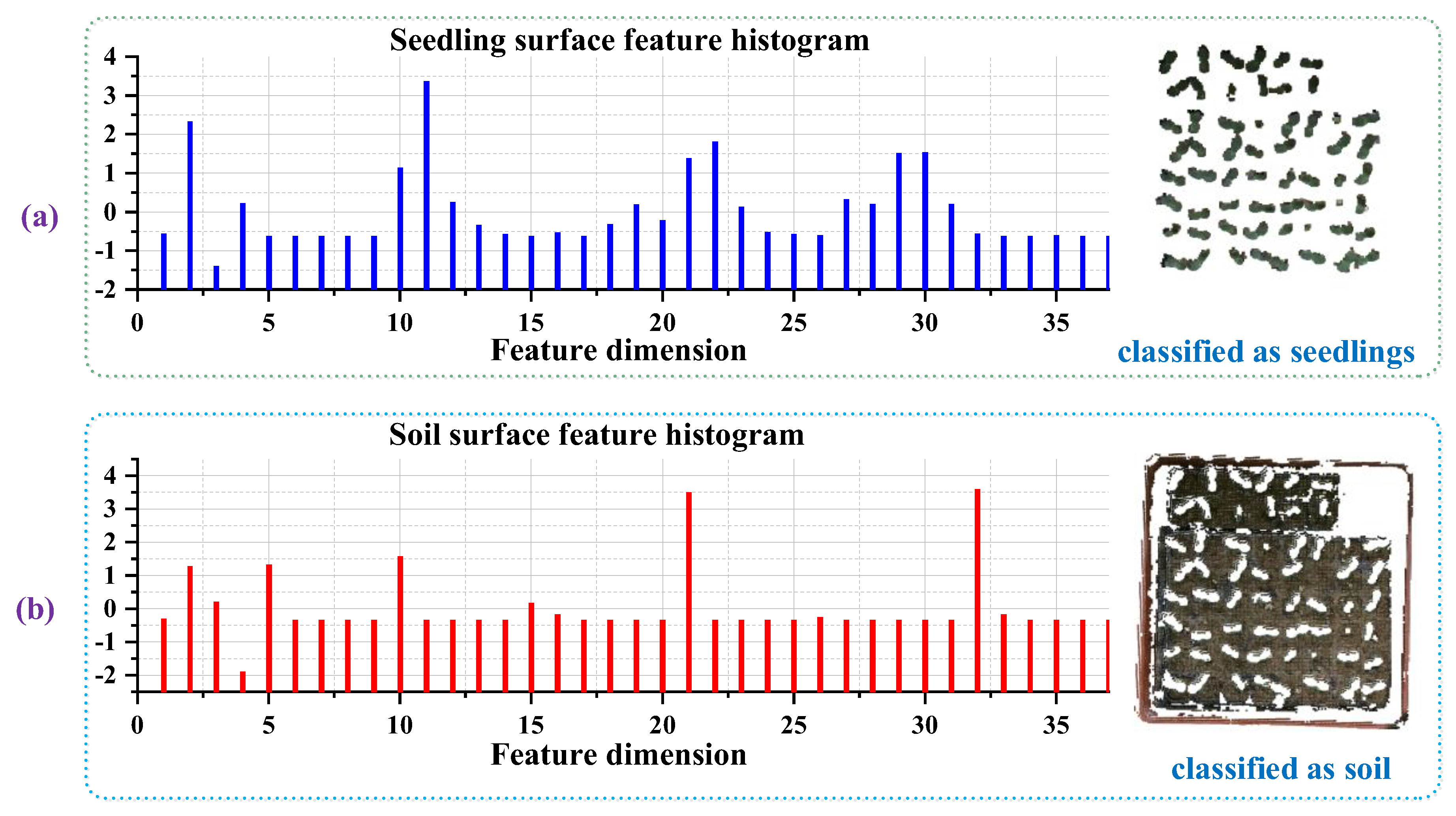
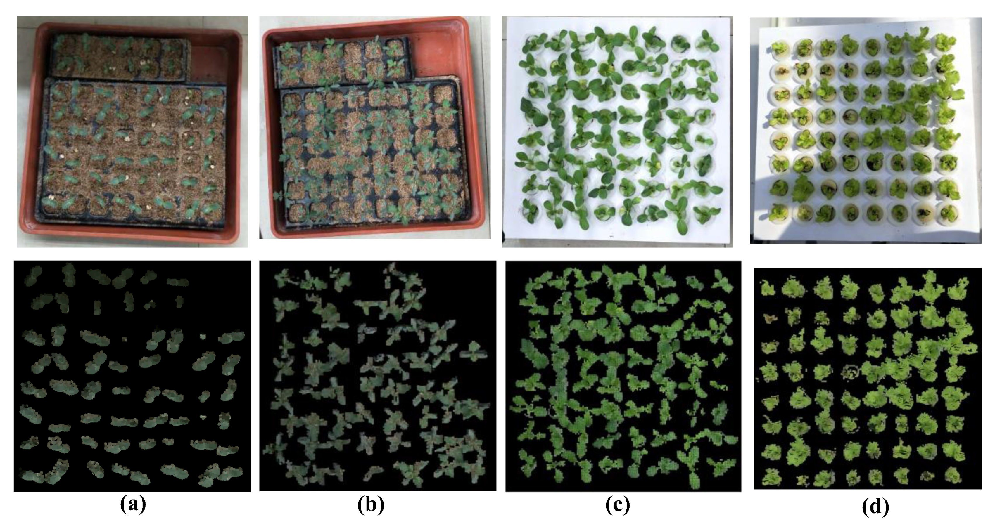
2.3. Removal of Natural Background

In plant phenotyping analysis, the segmentation of plants from the background was a crucial and challenging task [3,46]. Seedling segmentation from the background should be implemented prior to the segmentation of individual seedlings. Our captured data imply that it is difficult to remove the soil background simply according to the depth information or color information. Paulus et al. [47] used surface histograms for automated plant organ segmentation; however, its surface featured histograms of 120 dim, which increased the cost of computation and ignored color and spatial information, which could improve the robustness of algorithm. Rusu et al. [48] developed a 3D point clouds analyzing method using surface feature histograms for the demands of robotics and for the classification of low-resolution point clouds. The surface featured histograms, which provided a density- and pose-invariant description of the surface using properties of differential geometries, and were well suited for the real-time processing of point clouds data, and could be used for point clouds segmentation and the separation of different surface areas showing different surface properties [47]. In our study, an adapted surface featuring a histogram-based method was introduced for an automated pointwise classification of seedlings and soil background.
According to captured data, seedlings growing upon the soil, leading to the z values of seedling points, which were the distance between the sensor and seedlings on the z-axis, and were smaller than the soil points in our point clouds data. Additionally, we learned that the Hue–Saturation–Intensity (HSI) color space was commonly used for color-based segmentation, since it was more intuitive than red–green–blue (RGB) [49] and was more robust under complex illumination conditions. Thus, we introduced surface feature histogram adapted with depth and color information, together with a K-means algorithm as the method for the highly accurate separation of the natural background. In other words, the points of seedlings were automatically clustered in a 37-dimensional feature space, given as
F = [ z , H , S , I , F P F H 1 , 2 , , 33 ] ,
where z was the spatial coordinates on the z axis, H, S, I were color values in the HSI space, which could be efficiently converted from RGB values and F P F H 1 , 2 , , 33 were the 33 elements of Fast Point Feature Histograms (FPFH), a local geometrical feature proposed by Rusu et al. [48].
The characteristics of the FPFH of a single point depended on the radius for normal calculation r N and the radius for the histogram calculation r H . Both represented the number of neighbor points used for calculation. The variation in segmentation accuracy for r N , r H < 12 mm is shown in Figure 4. Our aim was to choose optimal parameters for our method. We determined r < r N < r H , with r representing the point clouds resolution. Furthermore, the resolution of the point clouds acquired by our platform was about 2.0 mm [41,44].
In this processing section, the pre-processed point clouds were classified into two clusters—one was seedling point clouds, the other was background point clouds. The classification results were validated using the manually segmented data. The classification accuracy was calculated using the following equation:
Accuracy = the true seedling points + the true background points the all pre-processed points ,
Reliable results have already been achieved with the combination of our adapted feature histograms and the clustering technique of the K-means algorithm. The removal of the natural background with the adapted surface feature histogram-based technique is shown in Algorithm 2.
Algorithm 2. Removing background with adapted surface feature histogram-based technique of pre-processed point clouds.
Input: pre-processed point clouds data (x, y, z, r, g, b in Euclidean space)
Output: seedlings point clouds data and background point clouds data
1. InputCloud ← pcloud % Putting the pre-processed point clouds data into the segmentation container
2. initialize and use kd-tree for efficient point access
3. r N ← 3.5% define radius for calculation of normal
4. r H ← 11.5% define radius for histogram calculation
5. for all points p in the point clouds do
6. calculate normal by using principal component analysis of points with radius r N
7. convert RGB into HSI
8. end
9. for all points p in the point clouds do
10. read coordinates of current point p (x, y, z, r, g, b)
11. find neighbor points p n with radius r H
12. for all neighbor points p n do
13. calculate F P F H 1 , 2 , , 33 histogram encoding the local geometry
14. end
15. combine z and H, S, I and FPFH as feature histogram and normalize
16. end
17. K-means ← 2% Setting the number of clustering
18. output seedlings point clouds and soil point clouds
The parameters of r N and r H were used to calculate the surface feature histogram, it was obvious that the surface feature histogram of seedlings was different from the natural background. In Figure 5, a detailed view of the classification of cucumber seedling point clouds and soil point clouds with a point clouds resolution of 2 mm is shown. Using r N = 3.5 mm and r H = 11.5 mm, an accuracy of about 99.97% was achieved. Figure 5a shows the 37-dim surface feature histogram of one seedling point, and the 37-dim surface feature histogram of one point of soil is shown in Figure 5b. Figure 5 illustrates the difference in the adapted surface feature histogram between point clouds with different surface properties, such as seedling leaves and soil. The left side shows a characteristic histogram for seedling leaves (a) and soil (b) that were calculated out of the clustering date and used for subsequent K-means clustering. The right shows the results of the clustering process of seedlings and soil after the K-means clustering step. In this experiment, we used cucumber seedling material to find the optimal parameters for the removal of the natural background. Then, we used the aforementioned parameter pair in other seedlings, and calculated the segmentation accuracy in different parameters in different types of seedlings. The ground truth of the natural background subtraction was manually segmented by MeshLab software (an Open-Source Mesh Processing Tool). The results (Table 2) shown that the choice of parameters had little relation to the plant type in our manuscript.

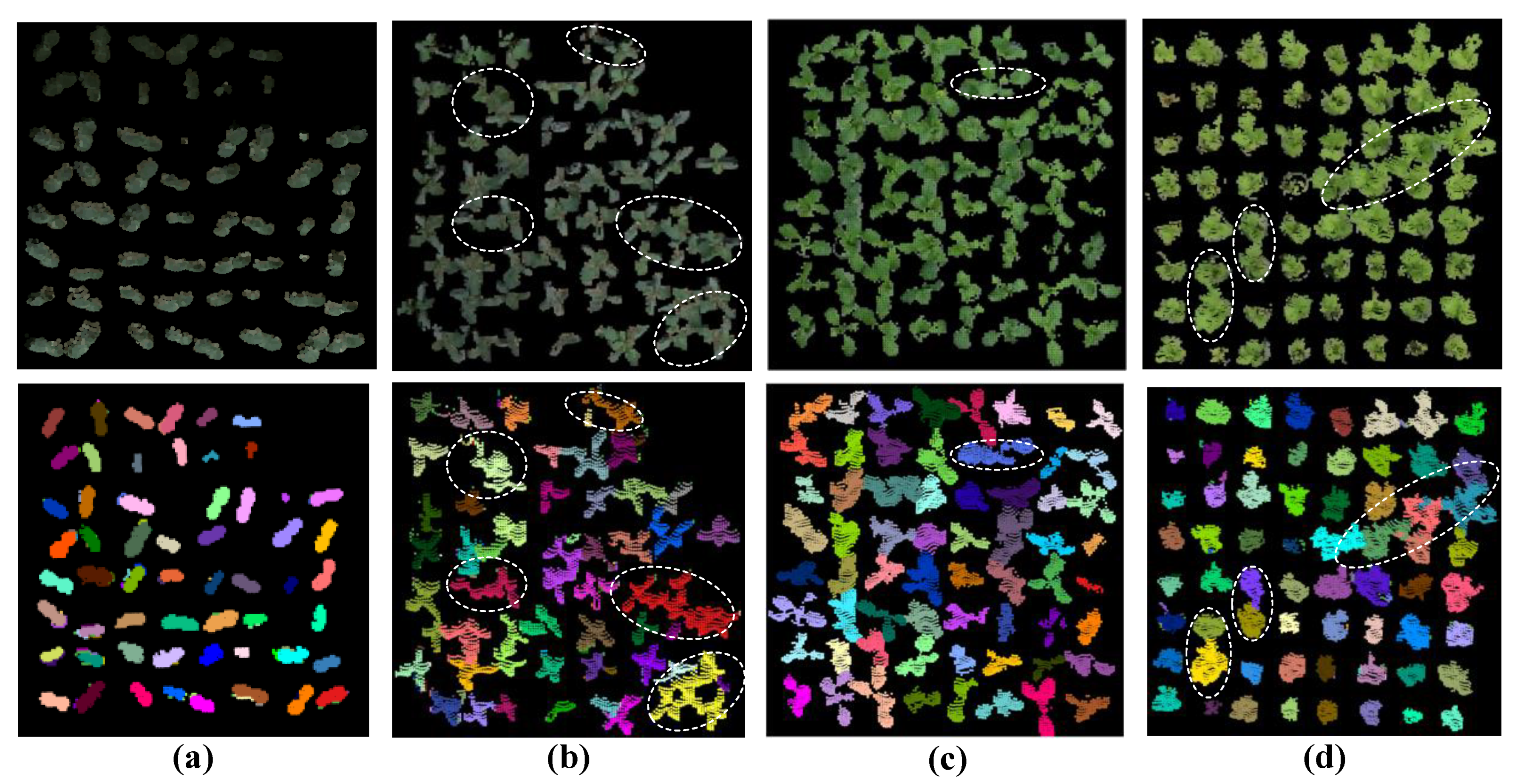
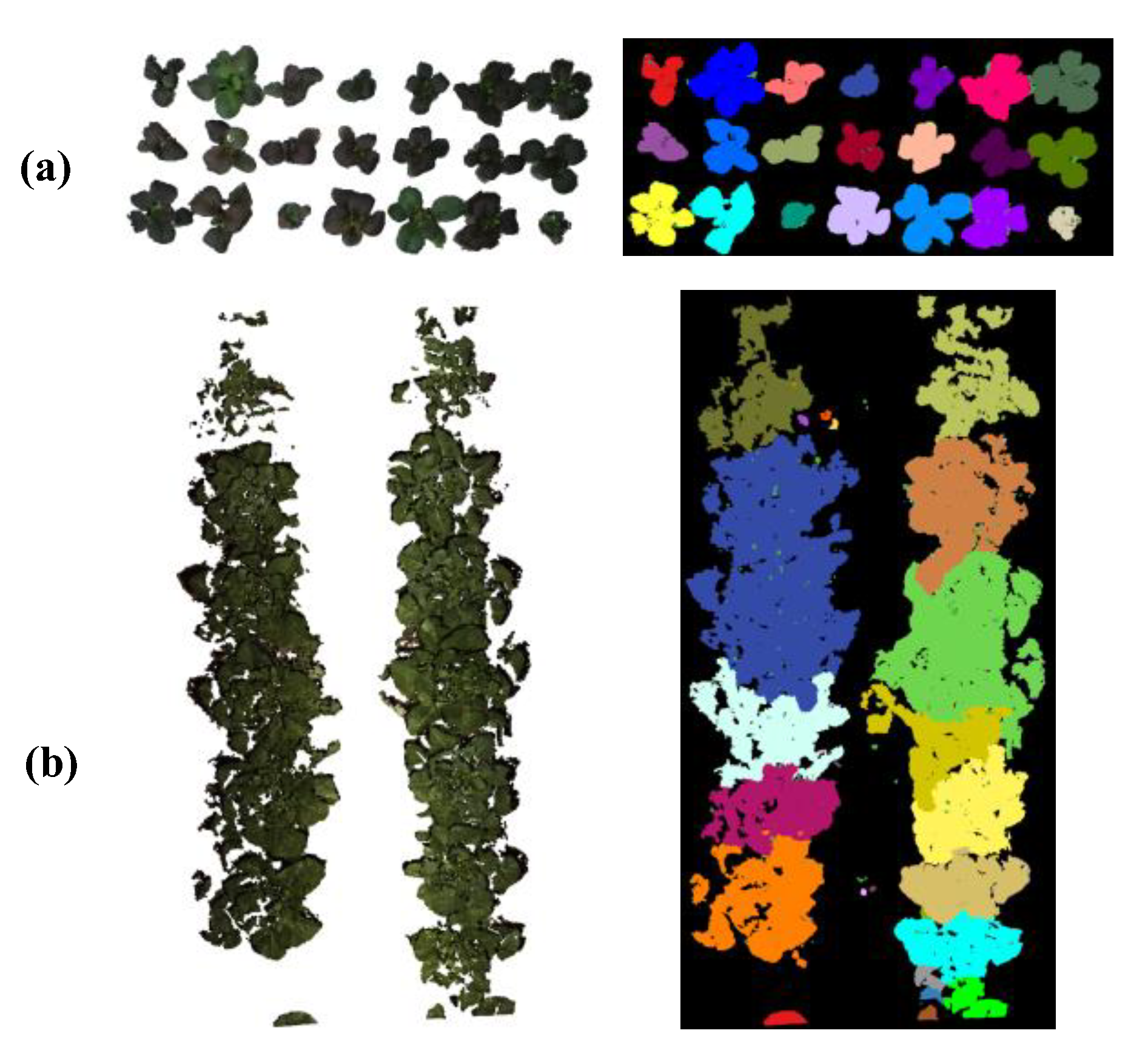
2.4. Segmentation of Individual Seedling

Individual seedling partitioning plays an essential role in high-throughput seedling phenotyping. In our study, for monitoring the growth of each seedling in a plug tray, we used Local Convex Connectivity Patches (LCCP)-based segmentation [50], which relied on local connectivity (convexity or concavity) between two neighbor patches to create rational segments (objects) for individual seedling clustering from the 3D colored point clouds.
First, we used Voxel Cloud Connectivity Segmentation (VCCS) [51], a novel method for generating super-pixels and super-voxels from 3D point clouds data, to build the surface–patch adjacency graph (super-voxel, a 3D analog of super-pixels). The octree data structure was used to create voxels, and the spatial relationship among voxels was established by an adjacency graph, which was generated by 26-neighborhood connectivity. In the voxelized space, after selecting seed voxels based on the seed resolution, these seed voxels grew to form super-voxels and distributed evenly. The super-voxel feature vector, which involved color, spatial, and the normal of points in each seed voxel, was initialized. The distance between the super-voxel center and the adjacent voxels in a considered search space was calculated by the equation:
D = λ D c 2 m 2 + μ D s 2 3 R s e e d 2 + ε D H i K 2 ,
where D c was the color distance in the CIELab space, normalized by a constant m. D s was the spatial distance, based on a distance of 3 R s e e d . D H i K was the distance in the FPFH space [48]. λ , μ , ε represented the influence of color, spatial and normal, respectively, in the clustering.
In our study, the color feature was incompatible with individual seedling isolation. We were interested in geometric features, such as the spatial weight μ = 4 and the normal weight ε = 1 . R v o x e l was slightly larger than the resolution of point clouds and much smaller than R s e e d , which approximately represented the distance between two neighbor seedlings. So, in the implementation of our algorithm, R v o x e l = 0.0038 , R s e e d = 0.018 . After VCCS, our point clouds data was over-segmented into super-voxels, which could not represent the true geometric characteristic of the seedlings. Realistic 3D segments were composed by merging appropriate super-voxels (Figure 6), each seedling was clustered and labeled in different colors. Thus, we implemented the Locally Convex Connected Patches (LCCP) algorithm [50] to calculate the geometrical connectivity between neighboring super-voxels. If two neighboring super-voxels satisfied the convexity criteria, the super-voxels could be merged into a segment object. For two neighboring super-voxels, S 1 , S 2 , their center position was x 1 , x 2 and their normal were n 1 , n 2 . The distance between S 1 and S 2 was d = x 1 x 2 . If ( n 1 n 2 ) · d > 0 , the local connectivity was convex. If ( n 1 n 2 ) · d < 0 , the local connectivity was concave. S 1 and S 2 would be merged if they satisfied the equation:
C C b ( S 1 , S 2 ) = ( n 1 n 2 ) · d > 0 ( β < β t h r e s h )
where C C b was the basic convexity criteria, β was the angle of n 1 and n 2 . β t h r e s h was a segmentation threshold which was used to merge concave super-voxels.
The partition of individual seedlings with VCCS and LCCP methods is shown in Algorithm 3.
Algorithm 3. Segmenting individual seedlings with Voxel Cloud Connectivity Segmentation (VCCS) and Locally Convex Connected Patches (LCCP) of seedling point clouds.
Input: seedlings point clouds data (x, y, z, r, g, b in Euclidean space)
Output: individual seedling point clouds data
1. InputCloud ← scloud %Putting the seedlings point clouds data into the segmentation container
2. initialize and use octree to create voxels
3. R v o x e l ← 0.0038% define radius for voxel
4. R s e e d ← 0.018% define radius for seed
5. μ ← 4% define the spatial weight
6. ε ← 1% define the normal weight
7. use VCCS to create super-voxels
8. β t h r e s h ← 10% define radius for histogram calculation
9. use LCCP for convex segmentation
10. output point clouds with each seedling labeled in different color

3. Results and Discussion

3.1. Removal of Natural Background

Before individual seedling phenotyping, seedlings in plug trays must be extracted from the background. The efficacy of the pre-processing and removal of the natural background was determined by analyzing the accuracy of seedling extraction from original top-view point clouds acquired by our experiment platform. An adapted surface feature histogram-based technique was implemented for an automated pointwise classification of seedlings and background, which included the root growth medium and plug tray. Fixed parameters, illustrated in Section 2.3, were used to segment seedlings from the background.
By testing these four different varieties of vegetable seedlings planted in two kinds of tray (soil culture and hydroponic) and two types of environment (plant factory and green house), all the seedling points could be extracted from the background. Figure 7 shows the removal of the natural background processing results for the four different vegetable seedlings—cucumber, tomato, pak choi cabbage and lettuce—grown in a plant factory or green house with a soil or hydroponic culture. The first row shows the original seedling RGB images captured by our platform; the second row shows the seedling point clouds extracted from the background. Our surface histogram-based method was robust in the greenhouse environment, with complex illumination conditions (Figure 7d), and was also robust in the complicated soil culture background (Figure 7a,b). The accuracies calculated by Equation (2) in four conditions were 99.97%, 95.46%, 97.61%, 96.42%, respectively, using r N = 3.5 mm and r H = 11.5 mm.
Then, we compared our adapted surface feature histogram-based algorithm to other algorithms with cucumber seedlings as the sample. The results of the segmentation accuracy and processing time costs of different surface feature histogram algorithms are shown in Table 3.
In addition, we supplemented more different experimental data. The first row of data was acquired by our platform in the greenhouse, the second were published by Mortensen et al. [26]. The removal of natural background results is shown in Figure 8.
Next, we will illustrate the reason why we chose four samples of four different varieties of vegetable seedlings planted in two kinds of trays and two types of environment. Firstly, we have verified that our algorithm is robust to different seedling species and both a greenhouse-like glass house and plant factory in IV. Secondly, we supplemented similar data to verify the robustness of our algorithm and revealed that our method can be extend to other, similar data.

3.2. Individual Seedling Segmentation Results

The proposed method using VCCS and LCCP algorithms was implemented to segment each cell seedling point cloud. Cucumber, tomato, pak choi cabbage and lettuce seedlings were used as samples to validate the robustness of the introduced methodology. The performance of the individual seedling partition was evaluated by the following equation:
Accuracy = The accurate identification seedlings number Total seedlings number × 100 %
The segmentation results for four different varieties of vegetable seedlings with two kinds of trays (soil culture or hydroponic) in two kinds of environments (green house or plan factory) are shown in Figure 9. The first row shows the seedling point clouds of four different seedlings after processing to remove the background; the second row shows the four species of seedling point clouds, with each seedling labeled in a different color after individual seedling isolation processing.
In Figure 9a,c, showing the cucumber seedlings and pak choi cabbage seedlings (the leaf shape is simple and elliptical), the accuracy of single seedling segmentation could reach 100% and 96.88%, but in Figure 9b, the accuracy of the needle-shaped tomato seedlings partition was only 75.00%. In Figure 9d, the irregular leafy lettuce seedlings could be partitioned correctly up to 95.31%; however, the edge segmentation of the leaves was still somewhat blurred and needed further improvement. Firstly, the resolution of our data acquired by our Kinect v2 platform was the main limitation that could not demonstrate information in detail, even though we tried our best to acquire high-precision data that only satisfied general plant phenotyping. The acquisition of high-precision plant 3D visual data needs further research. In addition, for point cloud segmentation, there was a fatal shortcoming: noise was unavoidable. There have been some point cloud segmentation works over the past two years, but it seemed that they still did not provide a good solution to these problems to the best of our knowledge. Whether there is a more direct segmentation method for 3D objects also requires further research.
In addition, we supplemented more different experimental data. The first data were acquired via our platform in greenhouse. The second data were published by Mortensen et al. [26]. The individual segmentation result is shown in Figure 10.
The segmentation accuracy was relatively low for the data in the second row. There are two main reasons—first, the vegetables were too densely planted, and it was difficult for human eyes to distinguish. This is a challenge for the computer vision method. Second, the point clouds of vegetable leaves acquired by Mortensen et al. [26] were inconsistent and uneven.
We could predicate that our individual seedling isolated method was more suitable for leafy vegetable seedlings whose leaf shapes are simple and elliptical.

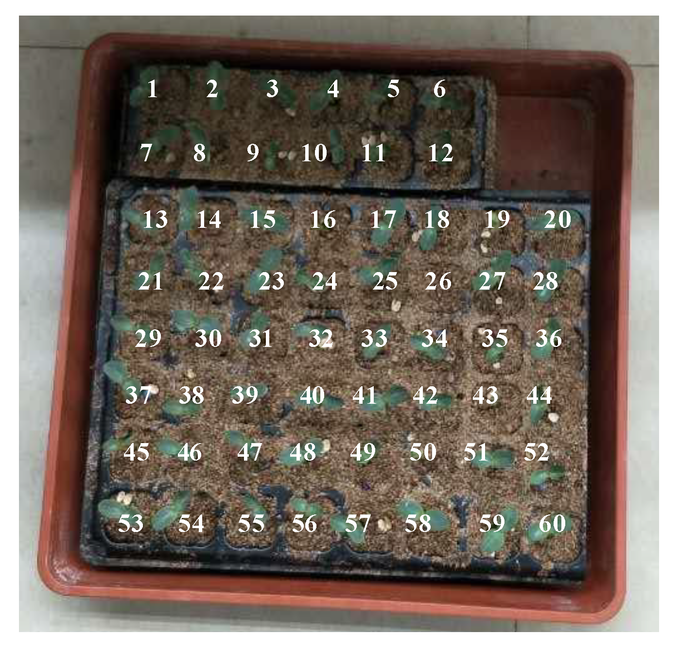
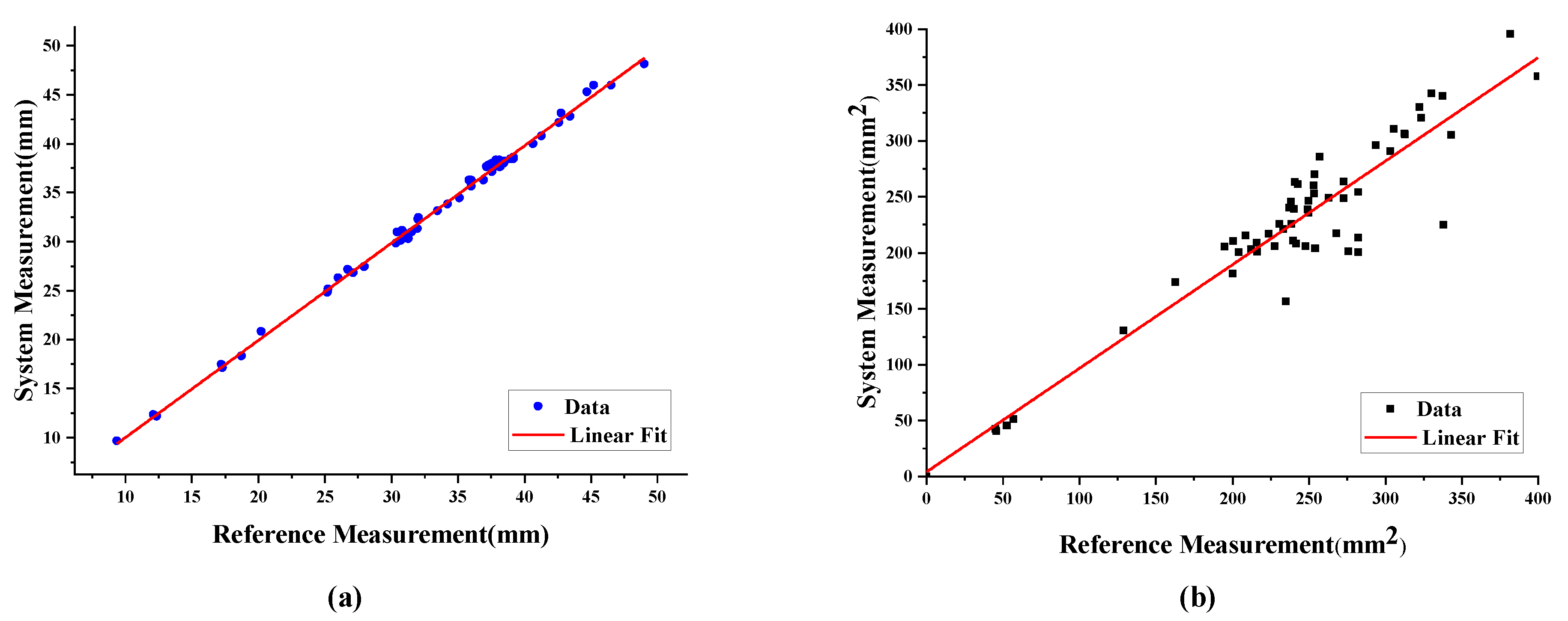
3.3. Height and Leaf Erea Estimation of Each Seedling

The proposed point cloud processing procedures were used to obtain high-throughput seedling phenotyping. Cucumber vegetable seedlings with soil culture in the greenhouse were tested, for example. Since single-seedling point cloud data have been accessed by previous processing, each single seedling growth parameter could be measured. The height and leaf area were measured by our system. The definition and principles of the system measurement method can be seen in Figure 11. The reference heights were measured by hand with a vernier caliper, whose resolution was 0.01 mm. The reference leaf areas were measured with a reference marker of known size by the original RGB image [31] captured by our platform.
In this paper, all cucumber seedlings in the plug tray were partitioned for the height and leaf area measurement experiment. Figure 12 showed that the cells of plug tray were labelled from left to right and from top to bottom.
The results of seedling height measurement and projected leaf area measurement for cucumber seedling samples are shown in Figure 13a,b. This shows that the system measurements, height (R2 = 98.22%) and projected leaf area (R2 = 89.28%), had a fine linear relationship with the reference data. The average measurement error of the cucumber seedling plant height is 2.30 mm, and the average measurement relative error is 7.69%. The filter preprocessing time is about 0.2 s, the background subtraction processing time is about 3 s, the time to segment the point cloud data by VCCS and LCCP is about 2 s, and the total time to obtain the plant height and leaf area of each cucumber seedling is about 2 s. Our method provided a novel high-throughput simultaneous acquisition technology for each single seedling height and leaf area and provided a new approach for high-throughput seedling phenotypic analysis.
The reasons for the measurement errors were as follows: (1) The manual measurement with a vernier caliper failed to make contact with the cucumber seedling in the middle of the seedling tray directly, resulting in a manual measurement error due to the vernier caliper. (2) Although the Kinect v2 camera was directly above the center plane of the seedling tray, the lens of the Kinect v2 sensor was not directly above all cucumber seedlings in the seedling tray. Therefore, the seedlings which were not directly below the Kinect v2 sensor tended to overestimate the seedling height. This was a systematic measurement error.
For the manual measurement error, other measurement tools can be used, such as a high-precision tape measure, etc., which can better contact the seedlings in the middle of the seedling tray, and reduce the manual measurement error. For the systematic measurement error, the spatial distribution of each seedling in the Kinect v2 coordinate system can be considered to reduce the systematic measurement error. Furthermore, a cone model field of view can be proposed to improve each seedling measurement accuracy.

3.4. Plant Height Precision Measurement

To validate the plant height measurement precision of the designed system, three differently sized and shaped plants (Succulents, Chlorophytum, Cyclamen persicum) with different distances to the Kinect v2 were taken to measure the plant height parameter, as shown in Figure 14. The experimental results of Figure 14 are, in turn, shown in Table 4.
The distance between the plant to be measured and the camera are set out in the range of 500 mm to 1000 mm, and the plant height precision of our method is 1~4 mm. Moreover, in our working distance of 750 mm, the plant height precision is about 2 mm.

3.5. Comparison with Similar Research

The main contribution of our research is that we proposed a low-cost processing pipeline for crop phenotypic data measurement and demonstrated the feasibility of the proposed approach. Recently, although more and more researchers have exploited the Kinect sensor to capture 3D point clouds and color images of plants, it still has difficulty in finding an absolute evaluation criterion to analyze each approach quantitatively due to the fact that each approach may concentrate on different aspect of phenotype tasks. We compared our study the latest paper [39], which is the most similar to our research, to illustrate the similarities and differences in date capturing, data processing and phenotypic data extracting.
For crop height measuring, Ma’s experiment and ours erected the Kinect v2 sensor above the plant in order to capture the whole canopy structure of the crop group because, in this setting, the Kinect data can retain the most real object depth, and effectively solve the problem of occlusion between other plants. Ma conducted their experiments outdoors, while our experiments were conducted indoors, in a greenhouse and plant factory. After understanding the performance limitations of Kinect v2 outdoors, we plan to conduct further research in the field with other RGB-D sensors, such as the Intel D435 sensor, which is unaffected by the light intensity and can be very useful in field agricultural applications.
The main difference of our research with Ma’s is 3D raw point cloud processing, including background removal and single plant segmentation. In Ma’s method for background subtraction, the 3D point cloud was back projected to the depth image and the background was removed according to the depth threshold. As Kinect v2 measures the depth by Time of Flight, for leafy crops it may introduce noise points at the leaf edges. Thus, removing the background directly according to the depth may result in the final height being inaccurate and interrupting the noise around the edge of the leaf. In our research, we proposed a 39-dim feature histogram, which was combined with depth, HIS and FPFH1…33 to describe each point, and then employed K-means algorithm to cluster the background points and crop group points, finally achieving the goal of removing the background and seedling tray. The feature histogram was driven from the depth, color and other features simultaneously; it not only removed background, but also the edge noise points. In order to segment individual crops, Ma’s method relied on the prior known parameters of regular placed pot and crop sizes, which imposed additional restrictions in data capture settings. However, with the VCCS and LCCP-based algorithms, individual crop segmentation was directly conducted, ignoring the crop growth and occlusion. In summary, our data processing pipeline was based on robust algorithms, while Ma’s employed pre-setting or empirical parameters. Thus, our approach is more universal than Ma’s.
The last comparison is related to phenotypic data extraction. As illustrated above, crop height is a key trait in plant phenotyping. Moreover, height measurement is a key advantage of employing an RGB-D sensor to capture the 3D point clouds, which revealed that our idea was consistent with Ma’s in height calculations. The other phenotypic data included leaf area in our research and canopy breadth and color indices in Ma’s.
The coincident aims of machine vision-based high-throughput plant phenotyping are to solve the time-consuming, labor-intensive and low accuracy characteristics of manual measurement. Both Ma’s research and ours have achieved this goal.

4. Conclusions

In this paper, we proposed a model- and learning- free bottom-up machine vision-based phenotyping acquisition workflow with low cost Kinect V2. Our method focused on the partition of individual seedlings in a plug tray to monitor seedling growth status for high-throughput seedling phenotyping. When macroscopically compared with other state-of-the-art segmentation methods, there was no need to create new training data and accompanying annotated ground truth data in our method. It was straightforward to implement, required no training data and was robust to the inconsistent illumination conditions. The results, which included time consumption and accuracy of measurement, were comparable to other methods. Our system can be extended from cucumber seedlings to non-acicular leafy seedlings with similar characteristics in which the shape features and texture patters are not complex. The height monitor of our method can be conducted with seedlings in which occlusion of each other seedling is not seriously, and the leaf area monitor can be conducted with young seedlings in which self-occlusion is not severe. Additionally, the precision of our measurement system is 2 mm and 4 mm2 for plant height and leaf area, respectively. For background subtraction, an adapted surface feature histogram-based method was introduced for an automated pointwise classification of seedlings and soil background. The adapted surface feature included HIS color space, depth value and 3D shape feature descriptors. It was obvious that the surface features of soil and the surface features of leafy seedlings were different. Thus, our system can be adaptive to various types of soil in terms of texture and color. For individual seedling segmentation, we used Local Convex Connectivity Patches (LCCP)-based segmentation, which relied on geometric features to partition individual seedlings. When one seedling was occluded by another seedling, and the local connectivity (convexity or concavity) between the leaves of two neighbor seedling was not remarkable enough to create a rational segment, the individual seedling partition did not perform well, and also affected the high-throughput phenotypic data extraction.
The major contribution and advantages of our method are: (1) the proposed experimental platform, which is convenient and can obtain fine canopy 3D colored point clouds for vegetable seedlings using a low-cost sensor. (2) The whole workflow of scanning, data processing and seedling phenotyping are automatic. (3) The method can be implemented without learning and modeling. (4) The system has generally good robustness in different environments and species of green leafy vegetable seedlings. (5) The method can be applied in high-throughput phenotyping research.
However, our approach has a few limitations. Firstly, the parameters of the involved individual seedling segmentation algorithms need to be set manually according to different environments and different seedlings. Secondly, since the obtained data was captured by our platform from a top view, we can only obtain the canopy information of vegetable seedlings.
Further works may include: (1) finding self-adaptive parameter deducting methods for the involved algorithms to make the system more flexible for different environments and different seedlings; (2) finding an algorithm to reconstruct the 3D models of plants to get more information about leaves; (3) making full use of the obtained 3D colored point clouds to study and gain more growth status information, such as stresses and diseases, so as to study the interaction between 3D plant phenotyping and environment and the interaction between 3D plant phenotyping and genotyping, which will alleviate the plant phenotypic bottleneck.

Author Contributions

S.Y., L.Z., W.G. and M.W. conceived and designed the experiments; B.W. and X.H. performed the experiments and acquired the 3D point cloud of seedling canopy; B.W., X.H. and J.M. calculated plant parameters; X.H. directed the seedling planting; S.Y. wrote the paper. All authors have read and agreed to the published version of the manuscript.

Funding

This study was funded jointly by National Natural Science Foundation (31471409), Project of Scientific Operating Expenses, Ministry of Education of China (2017PT19), the National Key Research and Development Program (2016YFD0200600-2016YFD0200602), the Key Research and Development Project of Shandong Province (2019GNC106091).

Acknowledgments

The authors would like to thank the three anonymous reviewers, academic editors for their precious suggestions that significantly improved the manuscript.

Conflicts of Interest

The authors declare no conflict of interest.

References

  1. Furbank, R.T.; Tester, M. Phenomics–technologies to relieve the phenotyping bottleneck. Trends Plant Sci. 2011, 16, 635–644. [Google Scholar] [CrossRef] [PubMed]
  2. Araus, J.L.; Cairns, J.E. Field high-throughput phenotyping: The new crop breeding frontier. Trends Plant Sci. 2014, 19, 52–61. [Google Scholar] [CrossRef] [PubMed]
  3. Tong, J.H.; Li, J.B.; Jiang, H.Y. Machine vision techniques for the evaluation of seedling quality based on leaf area. Biosyst. Eng. 2013, 115, 369–379. [Google Scholar] [CrossRef]
  4. Reynolds, M.; Langridge, P. Physiological breeding. Curr. Opin. Plant Biol. 2016, 31, 162–171. [Google Scholar] [CrossRef] [PubMed] [Green Version]
  5. Shakoor, N.; Lee, S.; Mockler, T.C. High throughput phenotyping to accelerate crop breeding and monitoring of diseases in the field. Curr. Opin. Plant Biol. 2017, 38, 184–192. [Google Scholar] [CrossRef]
  6. Pratap, A.; Gupta, S.; Nair, R.M.; Gupta, S.K.; Basu, P.S. Using plant phenomics to exploit the gains of genomics. Agronomy 2019, 9, 126. [Google Scholar] [CrossRef] [Green Version]
  7. Pieruschka, R.; Schurr, U. Plant phenotyping: Past, present, and future. Plant Phenomics 2019, 2019, 7507131. [Google Scholar] [CrossRef]
  8. Granier, C.; Tardieu, F. Multi-scale phenotyping of leaf expansion in response to environmental changes: The whole is more than the sum of parts. Plant Cell Environ. 2009, 32, 1175–1184. [Google Scholar] [CrossRef]
  9. Schurr, U.; Heckenberger, U.; Herdel, K.; Walter, A.; Feil, R. Leaf development in Ricinus communis during drought stress: Dynamics of growth processes, of cellular structure and of sink-source transition. J. Exp. Bot. 2000, 51, 1515–1529. [Google Scholar] [CrossRef] [Green Version]
  10. Vos, J.; Evers, J.; Buck-Sorlin, G.H.; Andrieu, B.; Chelle, M.; De Visser, P.H.B. Functional–structural plant modelling: A new versatile tool in crop science. J. Exp. Bot. 2009, 61, 2101–2115. [Google Scholar] [CrossRef]
  11. Paproki, A.; Sirault, X.; Berry, S. A novel mesh processing based technique for 3D plant analysis. BMC Plant Biol. 2012, 12, 63. [Google Scholar] [CrossRef] [PubMed] [Green Version]
  12. Leister, D.; Varotto, C.; Pesaresi, P.; Salamini, M. Large-scale evaluation of plant growth in Arabidopsis thaliana by non-invasive image analysis. Plant Physiol. Biochem. 1999, 37, 671–678. [Google Scholar] [CrossRef]
  13. Schmundt, D.; Stitt, M.; Jähne, B.; Schurr, U. Quantitative analysis of the local rates of growth of dicot leaves at a high temporal and spatial resolution, using image sequence analysis. Plant J. 1998, 16, 505–514. [Google Scholar] [CrossRef]
  14. Arend, D.; Lange, M.; Pape, J.M. Quantitative monitoring of Arabidopsis thaliana growth and development using high-throughput plant phenotyping. Sci. Data 2016, 3, 1–13. [Google Scholar] [CrossRef] [PubMed] [Green Version]
  15. Campbell, Z.C.; Acosta-Gamboa, L.M.; Nepal, N.; Lorence, A. Engineering plants for tomorrow: How high-throughput phenotyping is contributing to the development of better crops. Phytochem. Rev. 2018, 17, 1329–1343. [Google Scholar] [CrossRef]
  16. Watts-Williams, S.J.; Jewell, N.; Brien, C. Using high-throughput phenotyping to explore growth responses to mycorrhizal fungi and zinc in three plant species. Plant Phenomics 2019, 2019, 5893953. [Google Scholar] [CrossRef]
  17. Fiorani, F.; Schurr, U. Future scenarios for plant phenotyping. Ann. Rev. Plant Biol. 2013, 64, 267–291. [Google Scholar] [CrossRef] [Green Version]
  18. Sun, Q.; Sun, L.; Shu, M. Monitoring Maize Lodging Grades via Unmanned Aerial Vehicle Multispectral Image. Plant Phenomics 2019, 2019, 5704154. [Google Scholar] [CrossRef] [Green Version]
  19. Biskup, B.; Scharr, H.; Schurr, U. A stereo imaging system for measuring structural parameters of plant canopies. Plant Cell Environ. 2007, 30, 1299–1308. [Google Scholar] [CrossRef]
  20. Li, B.; Xu, X.; Han, J. The estimation of crop emergence in potatoes by UAV RGB imagery. Plant Methods 2019, 15, 15. [Google Scholar] [CrossRef] [Green Version]
  21. Duan, L.; Yang, W.; Huang, C. A novel machine-vision-based facility for the automatic evaluation of yield-related traits in rice. Plant Methods 2011, 7, 44. [Google Scholar] [CrossRef] [PubMed] [Green Version]
  22. Golzarian, M.R.; Frick, R.A.; Rajendran, K. Accurate inference of shoot biomass from high-throughput images of cereal plants. Plant Methods 2011, 7, 2. [Google Scholar] [CrossRef] [PubMed] [Green Version]
  23. Gehan, M.A.; Fahlgren, N.; Abbasi, A.; Berry, J.C.; Callen, S.T.; Chavez, L.; Doust, A.N.; Feldman, M.J.; Gilbert, K.B.; Hodge, J.G.; et al. PlantCV v2: Image analysis software for high-throughput plant phenotyping. PeerJ 2017, 5, e4088. [Google Scholar] [CrossRef]
  24. Zhou, J.; Applegate, C.; Alonso, A.D. Leaf-GP: An open and automated software application for measuring growth phenotypes for arabidopsis and wheat. Plant Methods 2017, 13, 117. [Google Scholar] [CrossRef] [PubMed] [Green Version]
  25. Tong, J.; Shi, H.; Wu, C. Skewness correction and quality evaluation of plug seedling images based on Canny operator and Hough transform. Comput. Electron. Agric. 2018, 155, 461–472. [Google Scholar] [CrossRef]
  26. Mortensen, A.K.; Bender, A.; Whelan, B. Segmentation of lettuce in coloured 3D point clouds for fresh weight estimation. Comput. Electron. Agric. 2018, 154, 373–381. [Google Scholar] [CrossRef]
  27. Li, L.; Zhang, Q.; Huang, D. A review of imaging techniques for plant phenotyping. Sensors 2014, 14, 20078–20111. [Google Scholar] [CrossRef]
  28. Vandenberghe, B.; Depuydt, S.; Van Messem, A. How to make sense of 3D representations for plant phenotyping: A compendium of processing and analysis techniques. OSF Prepr. 2018. [Google Scholar] [CrossRef] [Green Version]
  29. Ivanov, N.; Boissard, P.; Chapron, M. Computer stereo plotting for 3-D reconstruction of a maize canopy. Agric. For. Meteorol. 1995, 75, 85–102. [Google Scholar] [CrossRef]
  30. Yang, W.; Duan, L.; Chen, G.; Xiong, L.; Liu, Q. Plant phenomics and high-throughput phenotyping: Accelerating rice functional genomics using multidisciplinary technologies. Curr. Opin. Plant Boil. 2013, 16, 180–187. [Google Scholar] [CrossRef]
  31. Hu, Y.; Wang, L.; Xiang, L. Automatic non-destructive growth measurement of leafy vegetables based on kinect. Sensors 2018, 18, 806. [Google Scholar] [CrossRef] [PubMed] [Green Version]
  32. Jin, S.; Su, Y.; Gao, S. Deep learning: Individual maize segmentation from terrestrial lidar data using faster R-CNN and regional growth algorithms. Front. Plant Sci. 2018, 9, 866. [Google Scholar] [CrossRef] [PubMed]
  33. Jiang, Y.; Li, C.; Takeda, F. 3D point cloud data to quantitatively characterize size and shape of shrub crops. Hortic. Res. 2019, 6, 1–17. [Google Scholar] [CrossRef] [PubMed] [Green Version]
  34. An, N.; Welch, S.M.; Markelz, R.C.; Baker, R.L.; Palmer, C.; Ta, J.; Maloof, J.N.; Weinig, C. Quantifying time-series of leaf morphology using 2D and 3D photogrammetry methods for high-throughput plant phenotyping. Comput. Electron. Agric. 2017, 135, 222–232. [Google Scholar] [CrossRef] [Green Version]
  35. Seitz, S.; Curless, B.; Diebel, J.; Scharstein, D.; Szeliski, R. A Comparison and Evaluation of Multi-View Stereo Reconstruction Algorithms. In Proceedings of the 2006 IEEE Computer Society Conference on Computer Vision and Pattern Recognition—Volume 2 (CVPR 06), Washington, DC, USA, 6 June 2006; Institute of Electrical and Electronics Engineers (IEEE): Piscataway, NJ, USA, 2006; Volume 1, pp. 519–528. [Google Scholar]
  36. Bamji, C.S.; O’Connor, P.; Elkhatib, T. A 0.13 μm CMOS system-on-chip for a 512× 424 time-of-flight image sensor with multi-frequency photo-demodulation up to 130 MHz and 2 GS/s ADC. IEEE J. Solid State Circuits 2014, 50, 303–319. [Google Scholar] [CrossRef]
  37. Yamamoto, S.; Hayashi, S.; Saito, S. Proceedings of the Measurement of Growth Information of a Strawberry Plant Using a Natural Interaction Device, Dallas, TX, USA, 29 July–1 August 2012; American Society of Agricultural and Biological Engineers: St Joseph, MI, USA, 2012; Volume 1. [Google Scholar]
  38. Chéné, Y.; Rousseau, D.; Lucidarme, P. On the use of depth camera for 3D phenotyping of entire plants. Comput. Electron. Agric. 2012, 82, 122–127. [Google Scholar] [CrossRef]
  39. Ma, X.; Zhu, K.; Guan, H. High-throughput phenotyping analysis of potted soybean plants using colorized depth images based on a proximal platform. Remote Sens. 2019, 11, 1085. [Google Scholar] [CrossRef] [Green Version]
  40. Paulus, S.; Behmann, J.; Mahlein, A.K. Low-cost 3D systems: Suitable tools for plant phenotyping. Sensors 2014, 14, 3001–3018. [Google Scholar] [CrossRef] [Green Version]
  41. Fankhauser, P.; Bloesch, M.; Rodríguez, D.; Kaestner, R.; Hutter, M.; Siegwart, R. Kinect v2 for mobile robot navigation: Evaluation and modeling. In Proceedings of the 2015 International Conference on Advanced Robotics (ICAR), Istanbul, Turkey, 31 July 2015; Institute of Electrical and Electronics Engineers (IEEE): Piscataway, NJ, USA, 2015; pp. 388–394. [Google Scholar]
  42. Corti, A.; Giancola, S.; Mainetti, G. A metrological characterization of the Kinect V2 time-of-flight camera. Robot. Auton. Syst. 2016, 75, 584–594. [Google Scholar] [CrossRef]
  43. Yang, L.; Zhang, L.; Dong, H. Evaluating and improving the depth accuracy of Kinect for Windows v2. IEEE Sens. J. 2015, 15, 4275–4285. [Google Scholar] [CrossRef]
  44. Gai, J.; Tang, L.; Steward, B. Plant Localization and Discrimination Using 2D+3D Computer Vision for Robotic Intra-Row Weed Control. In Proceedings of the ASABE Annual International Meeting, Orlando, FL, USA, 17–20 July 2016; American Society of Agricultural and Biological Engineers: St Joseph, MI, USA, 2016; Volume 1. [Google Scholar]
  45. Vit, A.; Shani, G. Comparing RGB-D sensors for close range outdoor agricultural phenotyping. Sensors 2018, 18, 4413. [Google Scholar] [CrossRef] [PubMed] [Green Version]
  46. Xia, C.; Wang, L.; Chung, B.K. In situ 3D segmentation of individual plant leaves using a RGB-D camera for agricultural automation. Sensors 2015, 15, 20463–20479. [Google Scholar] [CrossRef] [PubMed]
  47. Paulus, S.; Dupuis, J.; Mahlein, A.K. Surface feature based classification of plant organs from 3D laserscanned point clouds for plant phenotyping. BMC Bioinform. 2013, 14, 238. [Google Scholar] [CrossRef] [PubMed] [Green Version]
  48. Rusu, R.B.; Blodow, N.; Beetz, M. Fast Point Feature Histograms (FPFH) for 3D registration. In Proceedings of the 2009 IEEE International Conference on Robotics and Automation, Kobe, Japan, 12–17 May 2009; Institute of Electrical and Electronics Engineers (IEEE): Piscataway, NJ, USA, 2009; pp. 3212–3217. [Google Scholar]
  49. Cheng, H.; Jiang, X.; Sun, Y.; Wang, J. Color image segmentation: Advances and prospects. Pattern Recognit. 2001, 34, 2259–2281. [Google Scholar] [CrossRef]
  50. Christoph Stein, S.; Schoeler, M.; Papon, J. Object partitioning using local convexity. In Proceedings of the IEEE Conference on Computer Vision and Pattern Recognition, Seattle, WA, USA, 16–18 June 2014; pp. 304–311. [Google Scholar]
  51. Papon, J.; Abramov, A.; Schoeler, M. Voxel cloud connectivity segmentation-supervoxels for point clouds. In Proceedings of the IEEE Conference on Computer Vision and Pattern Recognition, Portland, OR, USA, 23–28 June 2013; pp. 2027–2034. [Google Scholar]
  52. Rusu, R.B.; Marton, Z.C.; Blodow, N. Persistent point feature histograms for 3D point clouds. In Proceedings of the 10th International Conference Intelligence Autonomous System (IAS-10), Baden-Baden, Germany, July 2008; pp. 119–128. [Google Scholar]
Figure 1. Flowchart of the proposed individual vegetable seedling segmentation scheme. (a) The Indoor Scene at Plant Factory, (b) The Original Colored Point Cloud, (c) The Pre-processed Point Cloud, (d) The Seedlings Point Cloud, (e) The natural Background Point Cloud, (f) The Segmented Individual Seedling.
Remotesensing 12 01540 g001
Figure 2. Vegetable seedling growing environments and data capturing setting: (a) experiment platform in the greenhouse; (b) experiment platform in the plant factory.
Remotesensing 12 01540 g002
Figure 3. Key parameter optimization of filtering algorithms. In each row (ac), the left title is the filtering algorithm name with its key parameter(s) in parentheses, then follows the input point clouds and the results under three different parameter(s) settings, and the optimized values are underlined.
Remotesensing 12 01540 g003
Figure 4. Heat map for segmentation results according to different histograms and normal radius for pre-processed point clouds with a resolution of 2 mm.
Remotesensing 12 01540 g004
Figure 5. Surface feature histogram of (a) one point of cucumber seedlings and (b) one point of soil in 37-dim characteristic using r N = 3.5 mm and r H = 11.5 mm; 37-dim feature values were normalized, whose mean was zero and variance was one.
Remotesensing 12 01540 g005
Figure 6. Segmentation in different stages: (a) colored point clouds; (b) super-voxels; (c) segments. Parameters: R v o x e l = 0.0038, R s e e d = 0.0018, and β t h r e s h = 10°.
Remotesensing 12 01540 g006
Figure 7. Typical example of the removal of natural background processing results from four varieties of vegetable seedlings planted in different seedling trays and growing in two types of environment: (a) cucumber (b) tomato, (c) pak choi cabbage, (d) lettuce; (a,b) soil culture, (c,d) hydroponic; (ac) grown in plant factory, (d) grown in greenhouse. Parameters: r N = 3.5 mm, r H = 11.5 mm.
Remotesensing 12 01540 g007
Figure 8. The removal of natural background results in new experimental data. (a) the first row of data were acquired by our platform in the greenhouse, (b) the data of second row were published by Mortensen et al. [26] and acquired by stereo-configuration. The ground truth was segmented manually. The accuracies calculated by Equation 2 were 98.21% and 92.53%, respectively.
Remotesensing 12 01540 g008
Figure 9. Typical example of single seedling partition processing results from four varieties of vegetable seedlings planted in different seedling trays, grown in two types of environment: (a) cucumber (b) tomato, (c) pak choi cabbage, (d) lettuce; (a,b) soil culture, (c,d) hydroponic; (ac) grown in plant factory, (d) grown in greenhouse. Parameters: R v o x e l = 0.0038, R s e e d = 0.0018, and β t h r e s h = 10°.
Remotesensing 12 01540 g009
Figure 10. The individual segmentation result of new experimental data. (a) the data in the first row were acquired by our platform in the greenhouse, (b) the data in the second row were published by Mortensen et al. [26] and acquired by stereo-configuration. The accuracies calculated by Equation (5) were 100% and 61.54%, respectively.
Remotesensing 12 01540 g010
Figure 11. The definition and principle of system measurement method. (a) shows the definition of seedling height measurement, where Height1 and Height2 mean the distance between the Kinect sensor, seedling leaf and soil, respectively. Height is the seedling height; (b) shows the principle of seedling projected leaf measurement [31].
Remotesensing 12 01540 g011
Figure 12. Label of each seedling cell in plug tray.
Remotesensing 12 01540 g012
Figure 13. Data distribution and fitting results for cucumber seedling height (a) and projected leaf area (b).
Remotesensing 12 01540 g013
Figure 14. Three different plant sizes and shapes in validation experiment, (a) Succulents, (b) Chlorophytum, (c) Cyclamen persicum, and their manual measurement heights: 87 mm, 115 mm, 102 mm, respectively.
Remotesensing 12 01540 g014
Table 1. Field of view and spatial resolution at different working distances for top view [44].
DistanceField of View in mmSpatial Resolution in mm/pix
VerticalHorizontalVerticalHorizontal
<500 mmNot available
500 mm5777011.361.37
750 mm86610502.042.05
1000 mm115414002.722.73
Table 2. Optimal parameter pair for the removal of natural background in different vegetable seedlings.
Seedling TypeOptimal Parameter PairSegmentation Accuracy
r N r H
Cucumber3.511.599.97%
Tomato4.011.595.56%
Cabbage3.511.098.30%
Lettuce3.511.596.42%
Table 3. Results of segmentation accuracy and processing time costs of different surface feature histogram algorithms.
AlgorithmFeature DimensionAccuracy/%Time Costs/s
Ours3799.972.761
FPFH [48]3396.532.536
PFH [52]12585.2810.238
Paulus et al. [47]12598.8710.427
Table 4. Plant height precision measurement results of three different sized plants with different distances to the Kinect v2.
No.Distance to Kinect v2/mmSucculentsChlorophytumCyclamen Persicum
System Measure-Ment/mmMeasure-Ment Error/mmSystem Measure-Ment/mmMeasure-Ment Error/mmSystem Measure-Ment/mmMeasure-Ment Error/mm
15008431123993
255085211141002
360089211411042
465088111611064
570086111721053
675089211611002
78008611161993
885086111831002
990088111831031
1095088111721064
11100089211611042

