Land Cover Classification of Complex Agroecosystems in the Non-Protected Highlands of the Galapagos Islands

Abstract

The humid highlands of the Galapagos are the islands’ most biologically productive regions and a key habitat for endemic animal and plant species. These areas are crucial for the region’s food security and for the control of invasive plants, but little is known about the spatial distribution of its land cover. We generated a baseline high-resolution land cover map of the agricultural zones and their surrounding protected areas. We combined the high spatial resolution of PlanetScope images with the high spectral resolution of Sentinel-2 images in an object-based classification using a RandomForest algorithm. We used images collected with an unmanned aerial vehicle (UAV) to verify and validate our classified map. Despite the astounding diversity and heterogeneity of the highland landscape, our classification yielded useful results (overall Kappa: 0.7, R²: 0.69) and revealed that across all four inhabited islands, invasive plants cover the largest fraction (28.5%) of the agricultural area, followed by pastures (22.3%), native vegetation (18.6%), food crops (18.3%), and mixed forest and pioneer plants (11.6%). Our results are consistent with historical trajectories of colonization and abandonment of the highlands. The produced dataset is designed to suit the needs of practitioners of both conservation and agriculture and aims to foster collaboration between the two areas.

1. Introduction

1.1. The Humid Highlands of the Galapagos and Their Value

Vast expanses of agricultural land in the Galapagos have become abandoned in the last decades, making this UNESCO Natural World Heritage Site vulnerable to invasive plants, which thrive in disturbed environments [1,2]. Presently, the humid highlands of the Galapagos record higher numbers of invasive plants when compared to the dry lowlands, and these plants not only threaten agricultural systems but also the remaining patches of native-dominated ecosystems that still exist in the non-protected areas of this Ecuadorian archipelago [3]. Crop production and cattle ranching, when properly implemented, can effectively be used to control the spread of invasive plants or even rehabilitate invaded lands [4,5]. Given the direct influence of agriculture on both the introduction and control of introduced species, local governance seeks to incentivize agroecological models that serve to control the spread of invasive plants to nearby native dominated patches or to the protected lowlands while simultaneously contributing to local food security [5,6,7].

The humid highlands are also an irreplaceable foraging habitat for Galapagos giant tortoises and crucial nesting habitat for several endemic bird species [8,9]. Adult tortoises migrate every year from their nesting grounds in the lowlands to the highlands seeking food, and at high elevations, their seasonal diet has become dominated by introduced and invasive species [10]. Thus, some landowners of Santa Cruz island that are located in the tortoises’ migratory path have turned to tourism for their primary source of income, allowing tortoises to wander freely through their land and charging tourists to see tortoises in their “natural” environment [11]. However, land parcels are divided by barbed wire and living fences made up mainly of Erythrina smithiana. E. smithiana grows into dense thickets that act as barriers for tortoises and are known to interrupt their migratory paths [12].

1.2. Remote Sensing of Island Agroecosystems

Remote sensing techniques have become essential tools for agronomists and conservation scientists alike because they allow for systematic, non-intrusive, and uniform collection of data that can be interpreted from a biophysical standpoint, even in places that are hard to reach [13,14,15,16]. Despite its usefulness, remote sensing is still relatively underused because, until recently, access to high-resolution imagery was prohibitively expensive, and the long revisit time of high-resolution satellites was impractical for applications that required close monitoring, especially in regions with persistent cloud coverage [14,15]. However, this has changed with the introduction of small satellite constellations that have short revisit times and with the availability of freely-accessible high spatial and spectral resolution image collections [13,15,17].

The persistent cloud coverage, high biological diversity, and high landscape heterogeneity of island agroecosystems like those in the Galapagos make them challenging regions to classify. Among the plethora of methods, sensors, vegetation indices, and classification algorithms used for mapping island ecosystems and agricultural landscapes, methods that combine multiple data sources of complementary resolutions have been among the most successful at accurately classifying land cover [15,18,19,20,21]. The inclusion of vegetation indices is useful for differentiating land cover types that have variable spectral responses based on local conditions, such as moisture and vegetation health [16,22]. Object-based classification methods have been found to handle nuanced classification of high-resolution images better than pixel-based classification methods [15,18,23,24]. Machine learning methods, like decision trees [25], have become common and have been shown to have higher accuracy than parametric classification methods like maximum likelihood classifiers as they do not require assuming a particular statistical model for the distribution of the training data [24,25,26]. Object-based classification of high-resolution images using machine learning algorithms, like random forest, is an efficient method for classifying smallholder agricultural systems and mapping invasive species with high accuracy results [23,24,26,27,28]. Taking advantage of newly-available high-resolution sensors, commonly-used vegetation indices, object-based approaches, and contemporary machine learning methods, we can create an easily-replicable methodology that addresses the challenges of creating high-quality classification maps of regions like the humid highlands of the Galapagos.

1.3. Past and Present Efforts to Map the Humid Highlands and Agroecosystems of the Galapagos Using Remote Sensing

Despite the importance of the agricultural region for human wellbeing and environmental conservation, the land cover of these critical habitats remains mostly undocumented in detail for this tropical archipelago.

Table 1. Previous and current efforts to map land cover in the Galapagos Islands using remote sensing.*

Source	Sensor	Spatial Resolution	Spectral Resolution	Year Images Collected	Agricultural Zone Visibility
CLIRSEN and TNC, 2006	SPOT 4	20 m	Visible, SWIR	2000	highly obscured by clouds
	Landsat 5	30 m	Visible, NIR, SWIR	2000
SIGTIERRAS 2010	Orthophotos	0.5 m	Visible	2009	Yes
Rivas-Torres et al., 2018	Landsat 8	30 m	Visible, NIR, SWIR, Panchromatic	2015/2016	Excluded
	SRTM	30 m	Radar	2015
Jäger and Carrion (In press)	Worldview 2	0.46/1.84 m	Panchromatic, Multispectral	2015/2018	Excluded
Current publication	PlanetScope	3 m	Visible, NIR	2018	Yes
	Sentinel-2	10 m	Visible, Red Edge Edge, NIR, Narrow NIR, SWIR	2017/2019	Yes
	SIGTIERRAS DTM	10 m	Visible (Stereoscopy)	2009	Yes

CLIRSEN (Center for Integrated Survey of Natural Resources by Remote Sensing); TNC (The Nature Conservancy); SIGTIERRAS (Sistema Nacional de Información y Gestión de Tierras Rurales e Infraestructura Tecnológica); SPOT (Satellite Pour l’Observation de la Terre); SRTM (Shuttle Radar Topography Mission); DTM (Digital Terrain Model); SWIR (shortwave infrared); NIR (near infrared). * Shaded cells group used sensor types into individual studies.

summarizes previous and current efforts to map the Galapagos using remote sensing.

Most previous studies either exclude the agricultural areas or suffer from high cloud cover concentrations over the humid highlands (Table 1). Only the survey performed by the National System of Information of Rural Lands and Technological Infrastructure (SIGTIERRAS) has high-resolution images where the agricultural zone is visible. However, these images are a decade old, and the sensor was sensitive only to wavelengths within the visible spectrum. Furthermore, two of the primary studies that are used by the Galapagos National Park (GNP) and government institutions (CLIRSEN and TNC, 2006, and SIGTIERRAS 2010) are not published, so wider access to this valuable information is greatly restricted. Given the sensitive nature of ecosystems around and within the agricultural areas and the dynamic rate at which they change, it is imperative that the humid zones be precisely mapped with a replicable methodology to support monitoring efforts and to inform land management strategies [29].

1.4. Objectives

The purpose of this work is to build upon previous studies and make updated land cover classification maps of Galapagos agroecosystems available using some of the highest-resolution freely-available images. Specifically, our objectives for the present investigation are to:

• Develop a classification methodology, using remote sensing, specifically in complex agroecosystem landscapes.
• Identify regions of remaining native forests in and near the agricultural zone.
• Identify the distribution of invasive plant species like Psidium guajava, Rubus niveus, Zygsigum jambos, and Pennisetum purpureum that threaten agricultural lands and adjacent protected areas.
• Identify the distribution of Erythrina smithiana living fences in Santa Cruz, which might act as an obstacle for migrating tortoise populations.
• Identify the distribution of economically significant agricultural land cover like cattle ranching pastures, annual crops, tree crops, and cash crops, such as coffee.

Having access to updated information about the distribution of invasive species and remaining native forests will assist landowners and institutions like the GNP and the Ministry of Agriculture (MAG) in their goals to manage land uses, conserve protected species, and prevent the spread of invasive plants. Current land cover distributions can help determine the optimal conditions for prized crops, as well as predict the range of invasive plants in islands where plants may be at a different stage of colonization. This information, together with previous efforts using comparable mapping techniques, will help plan for future conditions as both local and global drivers, such as land use or climatic patterns, continue to change.

2. Materials and Methods

2.1. Study Area

All four inhabited islands of the Galapagos, Santa Cruz (−90.36387, −0.62881), San Cristobal −0.88422, −89.49595), Isabela (−0.80732, −91.01344), Floreana (−1.30986, −90.43528), have a zone in the humid highlands that has been designated for agricultural use (Figure 1). This region extends from what is commonly known as the “transition zone” at about 200 masl to some of the highest points of the islands (~700 masl). To define the study area, we created a 1 km buffer around the designated agricultural zone of each inhabited island. The buffer was included in the present mapping campaign to take into account the constant flow of people, animals, and plants across the boundary that separates the agricultural areas and the GNP [30].

The agricultural regions of the Galapagos face the south or windward side of the islands, which receive high levels of precipitation (813 mm mean annual precipitation) during the warm season (January–May) and remain enveloped in clouds during the cool season (June–December) [31]. The agricultural zones are within the humid highlands of the Galapagos, and in comparison to the lowlands, they receive nearly three times as much rain, present higher overall humidity (85–93% mean relative humidity, about 5% higher than the lowlands), lower average temperatures (16–20 °C mean minimum temperature, about 2 °C lower than the lowlands) and lower solar radiation (1–6 mean daily sunshine hours, about 2 h less than in the lowlands) throughout the year [32]. The humid highlands also record higher plant diversity when compared to the dryer lowland ecosystems of the Galapagos [31]. The severe seasonal temperature and precipitation fluctuations of highland areas have gradually weathered the islands’ volcanic rocks, creating a patchwork of nutrient-rich soils of variable depths and textures that can grow both tropical-weather crops and temperate-weather crops [33]. The greater primary productivity and diversity, combined with different edaphic conditions, have resulted in the formation of unique ecosystems that present distinct plant assemblages in comparison to the lower elevation arid areas [34]. Likewise, the unique conditions of the humid highlands harbor endemic plant species that present particular adaptations and biological mechanisms that are important to maintaining the ecological processes that characterize these ecosystems [35,36]. Such environmental uniqueness motivates prioritizing these areas for conservation within the renowned Galapagos archipelago [35,37,38].

Inhabitants of the highlands of the Galapagos devote their land to three general activities: cattle ranching, crop production, and tourism activities. According to the 2014 agricultural census, pastures cover nearly 60% of the land surface area of Galapagos agroecosystems, either cultivated or naturally germinated. A commonly grown variety is elephant grass (Pennisetum purpureum), which is used as cattle feed but is also considered invasive [39]. Pastures for cattle forage are often combined with forestry practices for tree crops or timber products, an agroecological practice known as silvopasture [36]. Tree crop varieties used in silvopastures often include lemon (Citrus spp.) or guava (Psidium guajava); P. guajava is also considered highly invasive. The most common transitory (annual) crops include maize, manioc, watermelon, and tomatoes, but these are reported to represent only about 1% of the surface area [40]. The most common permanent (perennial) crops are tree crops, such as coffee, banana, and plantain, but also pineapple and sugar cane. Reportedly, permanent crops cover about 8% of the surface area. Landowners reported that most permanent and transitory crops are grown as monocultures [41]. Pioneer (non-invasive but fast-growing) and forest species are reported to cover about 22% of the surface area, while invasive species (e.g., P. guajava, R. niveus, C. odorata, Zygsigum jambos) are reported to cover about 5% of the surface area in the agricultural region [40].

Farmers spend a great deal of time and resources clearing their land of invasive plants, which usually proliferate in vacant areas. Land parcels that do not have active land management sometimes become monocultures of invasive plant species, like guava (P. guajava) and cedar (C. odorata), which then spread into the adjacent protected areas. Invasive plants, which have severely modified 2–5% of the GNP, are mostly located in the humid highlands due to the higher productivity relative to the dryer lowlands [3,29,42].

2.2. Preliminary Definition of Land Cover Units

We focused on defining and mapping vegetation types that were of interest to both the conservation and agricultural sectors, including invasive species, like guava, and valued cash crops, like coffee. We based the agriculturally-relevant categories on those used by the 2014 agricultural census of the Galapagos [40]. Similarly, we based conservation-related categories on those used by the official classification systems of the MAG and on previous classification studies of the protected areas of the GNP [42,43].

We used level hierarchies to address the complexity of landscapes, breaking down broader categories into increasingly specific categories (Figure 2). At level 1, categories allow choosing between Land and the Pacific Ocean. At level 2, the ‘Land’ category is broken down into four categories: ‘bare ground,’ ‘built environment,’ ‘vegetation,’ and ‘freshwater.’ Bare ground is volcanic rock or soil surface area with no vegetation cover. This category excludes recently tilled land for crops. Built environment is surface covered by concrete, pavement, or other impervious surfaces. Vegetation represents all plants that cover the land surface, and freshwater describes naturally-occurring or artificial bodies of freshwater, such as ponds or reservoirs. At level 3, the ‘vegetation’ category is further broken down into ‘introduced’ and ‘native’ species, and levels 4 and 5 correspond to more specific categories that can be recognized as individual vegetation stands or patches at a mapping scale of 1:10,000. Introduced species (

Table 2. Descriptions of introduced land cover categories.

Category	Description
Cedrela—Cedar	Cedrela odorata, or spanish cedar, is a semi-deciduous tree 10–30 m tall, which outcompetes most other tree species and grows into a dense canopy [46].
Cinchona—Quinine	The red quinine tree (Cinchona pubescens) is a 15 m broad-leaved evergreen, which was once widespread in Santa Cruz’s Miconia region (~580 masl). [47]
Coffea—Coffee	The Coffea- and coffee category includes bushes of the arabica or robusta varieties since this is the most important cash crop and the only product that is exported. Coffee is often shade-grown with other tree crops like Citrus or banana (Musa spp.), so this category is limited to what is visible from above [40].
Cultivated Grass	Cultivated grass is a category that groups monocrops of less common cultivated grasses for pasture or landscaping, including grasses of Brachiara or Paspalum genera [40].
Erythrina— Porotillo	Erythrina smithiniana or porotillo is a shrubby tree of the Fabaceae family, which grows up to ~8 m and is commonly planted as stakes along the edges of farms to form ‘living fences’ [12].
Lantana–Supirosa	Lantana camara or Supirosa is an ornamental shrub up to 3 m tall that invades a wide variety of habitats, from tropical to temperate regions [48,49]
Mixed forest	Mixed forest is a category describing a forest where there is a mixture of introduced, invasive, or native species, and the dominance of a single species cannot be established [42].
Permanent Crops	Permanent Crops are those that take over one year to reach productive age, and that can produce for several subsequent years without requiring replanting after each harvest. Some of the most common perennial crops include coffee (Coffea spp.), plantain, banana (Musa spp.), sugar cane (Saccharum spp.), pineapple (Ananas spp.), and orange (Citrus spp.) [40]. The permanent crops category also includes all other perennial or tree crops, such as pineapple (Ananas spp.), sugar cane (Saccharum spp.), or other tree crops, commonly of Fabaceae, Persea, or Carica genera [40].
Pennisetum—Elephant grass	Pennisetum purpureum or Elephant grass is the most common type of cultivated grass for cattle fodder and grows tall, robust bamboo-like clumps [40].
Psidium—Guava	Psidium guajava or guava is a small tree (8 m tall) that has escaped cultivation and become common in mesic forests (>150 masl) of several of the large islands [50,51].
Rubus—Blackberry	Rubus niveus or blackberry is a widespread thorny shrub that grows in gaps of native vegetation and forms dense thickets up to 4 m high over grasslands, bracken, bush, and forest areas alike [52].
Silvopasture	Silvopasture describes an intentional combination of pasture for cattle grazing and trees, which provide additional fodder for cattle, fruit crops, wood, or shade [53].
Syzygium—Pomarrosa	Syzygium jambos or pomarrosa is a small tree (3—15 m) that forms dense thickets and threatens several highland habitats, especially in San Cristobal and Isabela [2].
Transitory Crops	Transitory crops are short-cycle crops. Common ones include maize (Zea spp.), cassava (Manihot spp.), and watermelon (Citrullus spp.) [40].

) are plants that were intentionally or unintentionally brought to the islands by humans and have become naturalized since their introduction, such as Citrus and Erythrina spp. Native species (

Table 3. Descriptions of native land cover categories.

Category	Description
Deciduous Forest	Deciduous forest was sometimes referred to as ‘dry or arid zone’; this area is mostly lava substrate dominated by native species like Acacia spp., Bursera graveolens, Piscidia carthagenensis, Croton scouleri, or Opuntia spp., and ranges from 0 to ~200 masl [42,46].
Evergreen Forest and Shrubland	The Evergreen forest and shrubland is sometimes referred to as the ‘Scalesia’, ‘brown’, and ‘Miconia’ zones. This region contains well-developed soil with vegetation characterized by an abundance of shrubs, herbs, ferns, and trees like Darwiniothamnus tenuifolius, Lycopodium spp., Scalesia pedunculata, Miconia robinsoniana, and Zantoxylum fagara. Epiphytes like mosses and liverworts commonly cover the trunks and branches of trees in this zone [42,46,51].
Evergreen Seasonal Forest and Shrubland	Evergreen seasonal forest and shrubland is an ecosystem previously referred to as ‘transition zone’, where soil and understory are more developed than the deciduous forest and species like Clerodendrum molle, Cordia lutea, Chiococca alba, Psidium galapageium, Tournefortia spp. can be found [42,46,51].
Humid Tallgrass	Humid tallgrass is a region previously known as ‘pampa zone’, which contains virtually no trees or shrubs, and its vegetation consists mainly of ferns, grasses, and sedges like Cyathea weatherbyana, Habenaria monorrhiza, or Pteridium aquilinum [42,43].
Pioneer	The pioneer category describes herbaceous, quick-growing native vegetation that thrives in recently disturbed areas, such as Plumbago scandens, Senna occidentalis, Mentzelia aspera, Sida rhombifolia, or Heliotropium spp., but likely also includes introduced herbaceous species like Amaranthus spp., or Pothomorphe peltata [46].

) are those that arrived on the islands by their own means, transported by the wind, water, or other animals [44]. Introduced species include food crops (transitory and permanent crops), pastures, and invasive species. The pastures category includes grass species planted by farmers for cattle grazing naturally-occurring species that are dispersed by the wind [40]. Invasive species are a subset of naturalized plants that produce reproductive offspring in large numbers and over a considerable distance, thus having the potential to spread over large areas and negatively impact native biota [45]. Some of the most common and aggressive species include Cedrela odorata (cedar), Cinchona pubescens (quinine), Psidium guajava (guava), Rubus niveus (blackberry), Lantana camara (supirosa), and Syzygium jambos (pomarrosa) [42].

2.3. Land Cover Classification

A detailed description of the mapping process is found in Figure 3 and the sections below.

2.3.1. Data Acquisition

Multispectral Data

New freely-available sensors, such as the 10-meter spatial resolution Sentinel-2 images from the UE’s Copernicus Programme [54], and 3-meter spatial resolution 4-Band PlanetScope images from Planet Labs [55], can help overcome the challenges that have limited mapping of these areas. Planet Labs is a commercial venture, but its image collections are accessible to university students and faculty for free through its education and research program.

PlanetScope sensors have a high spatial resolution (3 m) and are sensitive to both visible and Near Infrared (NIR) wavelengths (Figure 4). The high spatial resolution of PlanetScope images allows visualizing considerably more details than NASA’s freely available Landsat collections or even commercially-available SPOT (Satellite Pour l’Observation de la Terre) sensors. Meanwhile, Sentinel-2 sensors have a high spectral resolution (Aerosol, Visible, Red Edge, NIR, Narrow NIR, Water Vapor, and Short Wave Infrared or SWIR) and have a 10, 20, and 60-meter spatial resolution (Figure 4).

The multispectral images used to make the mosaic and land cover classification are listed in

Table 4. Multispectral images used for land cover classification of the Galapagos agricultural zone.

Sensor	Capture Date	Capture Time	Visible Islands	Cloud Cover (%)
Sentinel-2	21-February-17	11:33:01 AM EST	Isabela, Santa Cruz, Floreana	0
Sentinel-2	10-March-19	12:23:11 PM EST	San Cristobal	22
4-Band PlanetScope	10-March-18	10:47:46 AM EST	Floreana	0
4-Band PlanetScope	10-March-18	10:46:47 AM EST	Floreana	0
4-Band PlanetScope	11-April-18	11:52:07 AM EST	Isabela	0
4-Band PlanetScope	11-April-18	11:52:08 AM EST	Isabela	0
4-Band PlanetScope	11-April-18	11:52:09 AM EST	Isabela	0
4-Band PlanetScope	9-March-18	10:48:35 AM EST	Santa Cruz	1
4-Band PlanetScope	9-March-18	10:48:36 AM EST	Santa Cruz	1
4-Band PlanetScope	9-March-18	10:48:37 AM EST	Santa Cruz	0
4-Band PlanetScope	10-March-18	10:47:34 AM EST	Santa Cruz	0
4-Band PlanetScope	10-March-18	10:47:35 AM EST	Santa Cruz	0
4-Band PlanetScope	10-March-18	10:47:36 AM EST	Santa Cruz	0
4-Band PlanetScope	10-March-18	10:45:18 AM EST	San Cristobal	2
4-Band PlanetScope	10-March-18	10:45:19 AM EST	San Cristobal	1
4-Band PlanetScope	31-March-18	11:44:57 AM EST	San Cristobal	1
4-Band PlanetScope	31-March-18	11:44:58 AM EST	San Cristobal	7

. These images were chosen by searching through Planet and Copernicus image collections for low (usually <10%) cloud cover images from the warm/humid season (January–May) that were recorded less than a month apart from each other for each island to avoid variability in the island mosaics. Even if cloud cover was greater than 10%, the images were considered useful if land areas were visible. Images from 2018 were used as a reference, and we included images a maximum of one year apart to complete areas that suffered from cloud coverage.

Topographical Data

We used a 10-meter spatial resolution Digital Topographic Model (DTM) generated from SIGTIERRAS orthophotos (2010). The DTMs were provided by authorities from the Galapagos Government Council (CGREG). Elevation and Slope are useful predictors of vegetation variability [56,57]. We calculated the slope from the DTM layer in ArcMap.

Unmanned Aerial Images and GPS Control Points

From 2017–2019, we surveyed about 83 agricultural production units (UPA) on all four islands. Most surveyed UPAs were recommended for mapping by MAG because they are considered to be representative of agrarian production on each island. Additionally, some UPAs were chosen because they are located in known tortoise habitat. During the surveys, we collected high-resolution (<2 cm per pixel) visible wavelength images of the UPAs with an unmanned aerial vehicle (UAV—DJI Mavic Pro Platinum, 1/2.3 CMOS Sensor), as well as 826 control points of the most salient landscape features and vegetation types within the UPAs that were visible from above, wherever terrain accessibility allowed, using a handheld GPS (Garmin Map64, accuracy: +/− 3 m). We covered an area of ~1252 ha with our drone flights, corresponding to about 2% of the study area (

Table 5. Extent of surveyed area per island.

Island	Number of UPAs Surveyed	UAV Survey Area (ha)	Percentage of Study Area
Santa Cruz	26	566.89	1.92
San Cristobal	38	503.37	2.92
Isabela	12	124.18	0.98
Floreana	7	57.85	3.35
All islands	83	1252.29	2.05

, Figure 5). We aligned the UAV images and generated a three-dimensional mesh that we used to stitch together a high-resolution (~0.04 m) orthomosaic using AgiSoft Photoscan (version 1.4.5) for each UPA.

2.3.2. Image Pre-Processing

We used PlanetScope surface reflectance products, which were already atmospherically corrected to bottom-of-atmosphere reflectance. We generated the mosaic of these scenes in ENVI 5.3 and applied a 20-pixel edge feathering between images. Sentinel-2 images were atmospherically corrected in SNAP 6.0 using the Sen2Cor plugin with a Maritime setting. Lastly, we enhanced Sentinel-2’s 20 m and 60 m bands to 10 meters using Sen2Res [58]. The Sen2Res algorithm separates band-dependent information (reflectance) from information that is common to all bands (geometry of image elements), then unmixes lower resolution bands, maintaining their reflectance while propagating the geometry of scene elements to keep sub-pixel details [58]. All multispectral image mosaics, the DTM, and slope layers were clipped using a mask of the study area. The Sentinel-2 images were used as a reference for orthorectification of the PlanetScope images.

2.3.3. Image Fusion

We used the variational fusion method proposed by Gasparovic et al. (2018) to fuse PlanetScope and Sentinel-2 images to improve classification accuracy. This method introduces the geometry information of the higher resolution image (PlanetScope) by aligning all edges of the higher resolution bands with each lower resolution (Sentinel-2) multispectral bands of similar spectral characteristics [59,60]. Figure 4 highlights the spectral overlap with Sentinel-2 and PlanetScope fused bands. High-resolution PlanetScope bands 1, 2, 3, and 4, were each fused with the 10 m Sentinel-2 bands 2, 3, 4, and 8, respectively. We also fused PlanetScope’s Band 4 with Sentinel’s Band 8A, 11, and 12. There is no direct equivalent to fuse with Sentinel-2’s Red Edge bands, so following Gasparovic et al. (2018), we generated a synthesized band (S) using Equation (1),

$$S=\frac{B3+B4}{2}$$

(1)

where B3 is PlanetScope’s Band 3 (Red), and B4 is its Band 4 (NIR).

Table 6. Band combinations for fusing PlanetScope with Sentinel-2 images.

		PlanetScope
	Bands	B1—Blue	B2—Green	B3—Red	B4—NIR	S—Syn
Sentinel-2	B2—Blue	X
	B3—Green		X
	B4—Red			X
	B5—Red Edge					X
	B6—Red Edge					X
	B7—Red Edge					X
	B8—NIR				X
	B8A—Narrow NIR				X
	B11—SWIR				X
	B12—SWIR				X

summarizes the band combinations that were used to obtain the fused images. Image Fusion was conducted with the open-source Orfeo ToolBox V.6.6.1.

2.3.4. Vegetation Indices

The fused multispectral images were used to generate vegetation indices, namely the Normalized Difference Vegetation Index (NDVI), Structural Index (SI), and Normalized Difference Vegetation Red Edge (NDRE). NIR wavelengths are used to calculate vegetation indices like the NDVI and SI, which are known to be useful for land cover classification [22,61,62]; studies also suggest that including Sentinel-2’s Red Edge band in a vegetation index, such as the NDRE, can yield more accurate results for the classification of agricultural areas [16,63].

2.3.5. Object-Oriented Classification with RandomForest

Random Forest (RF) is a widely used algorithm for remote sensing, being a powerful option for integrating different imagery sources and ancillary data sources into image classification workflows [64,65]. RF classification has been demonstrated to work well in land cover classification tasks like this one because it is effective with relatively small samples of training data and not particularly sensitive to noise [27]. The method is also ideal because it can achieve good accuracy without detailed hyperparameter optimization, and provides a robust estimate of the trained model’s uncertainty [23,24,27].

Segmentation

We created the objects with a multiresolution algorithm where PlanetScope bands and fused Sentinel-2 bands (Red, NIR) were given equal weight. The images were divided into segments of relatively homogenous pixel composition, where the mean of band values of pixels within each segment is used to represent “objects.” We set the segmentation scale parameter at 40 pixels, where each pixel is about 9 m². During the segmentation process, the similarity of pixels was determined by two values ranging from 0 to 1. The first value is a shape criterion, where higher values mean that the color of pixels is given less influence over what is included or excluded from each segment. The second value is a compactness criterion, where higher values emphasize spatial proximity, causing resulting objects to be more compact. We used a trial-and-error approach to determine the values (shape: 0.7; compactness: 0.3) where objects such as built environment, living fences, and pastures were selected most completely while excluding adjacent objects of different categories.

Training Data Sample

On each island, at least 20 object samples were selected for each category using GPS control points and drone images acquired during fieldwork as reference. These object samples represent areas where the cover category covers the total extension of the sample. From this data sample, we selected 50 stratified random pixel sample subsets for training the classification model.

Random Forest Classification

RF classification was performed in R Studio open-source statistical software, where we used the randomForest, Caret, and raster packages to produce all classifications. For each island classification, randomForest sampled 1000 classification trees and tried four variables at each split to calculate the out-of-bag samples (rfOOB). The rfOOB are used to create a cross-validated prediction error for the model and to formulate a measure of feature importance [66].

We used two sets of metrics to gauge the importance of 20 different variables from three different sources (orthophoto, PlaneScope, Fused S2 + PS;) in the randomForest model. The first metric we used is the Variable Importance (Caret Package), which is the mean of the scaled (from 0–100) class-specific decreases in accuracy. The second set of metrics we used included the Mean Decrease Impurity Importance (MDI) or Mean Decrease in Gini, as well as the Mean Decrease Accuracy (MDA, randomForest package). MDI measures how important a variable is for estimating the value of a target class across all of the decision trees that make up the forest. MDA evaluates the importance of each variable by looking at how much prediction error increases when removing that variable while all others are left unchanged [67,68].

2.3.6. Verification

Throughout the image classification process, we used Google Earth, high-resolution UAV images, GPS control points, and expert knowledge to inform, correct, and fine-tune the training samples for the image classification. We ran the classification algorithm multiple times, and after each iteration, we identified regions where we suspected the classification had issues, and then selected additional samples or removed existing samples to correct our results. Categories with insufficient data (Lantana, Erythrina) to select training samples that would produce consistent results were dropped from the classification.

2.3.7. Validation

To validate the map, we created a confusion matrix and calculated Cohen’s Kappa [69,70,71]. We also calculated the receiver operating characteristic (ROC) area under the curve (AUC) for our land-cover methods, which is sometimes used to demonstrate the accuracy of machine learning methods [72]. However, this metric assumes that grid contents are homogenous. Given that we are dealing with high-resolution data and land cover classes that are often not discrete, we also assessed the accuracy of our maps by calculating the root mean square error (RMSE) and a correlation coefficient (R²) like land cover classification studies that use high-resolution images [73,74,75,76].

First, we generated a grid of 60 × 60 m squares. We randomly selected 15 squares on each island that overlapped areas where we had high-resolution images and control points but that did not overlap with the areas chosen for training the algorithm. This way, we maintained independent data sources for the geometry of the classified images and our reference polygons [69]. We created two versions of these areas, one to serve as the reference polygons and the other to serve as the prediction. We intersected the prediction polygons with the classified maps to extract the information corresponding to those areas. For the reference polygons, we cut them into sections that visually matched the high-resolution UAV images and the GPS control points, and we manually classified them.

To characterize the effectiveness of our classification for estimating land cover fractions, we calculated the percentages of the polygons that were occupied by the different classes, and obtained a root mean square error (RMSE) and a correlation coefficient (R²) for each island and for each class c using Equations (2) and (3) [73,74,75,76], respectively:

$$RMSE\left(c\right)=\sqrt{\frac{1}{N}{{\displaystyle \sum }}_{i=1}^N{\left({\widehat{f}}_{i,c}-f_{i,c}\right)}^2},$$

(2)

$$R^2{}_c=\frac{{{\displaystyle \sum }}_{i=1}^N{\left(\widehat{f_{i,c}}-{\overline{f}}_c\right)}^2}{{{\displaystyle \sum }}_{i=1}^N{\left(f_{i,c}-\overline{f_c}\right)}^2}$$

(3)

where $\widehat{f_{i,c}}$ is the predicted land cover fraction of class c for sample i, $f_{i,c}$ is the true land cover fraction of class c for sample i, $\overline{f_c}$ is the mean class c land cover fraction of the samples, and N is the total number of samples. If the predicted cover perfectly matched the reference cover, we would expect an R² value of 1 and an RMSE of 0 for that class. The island-wide results were obtained by summing simultaneously over samples and classes in Equations (2) and (3).

The AUC is a performance metric that estimates how well a model is able to distinguish between classes, typically ranging between 1 (perfect classification) and 0.5 (no predictive capability); values less than 0.5 are characteristic of a classifier that is anticorrelated with the true categories [77,78]. The AUC only characterizes binary predictors, so we calculated the AUC values for each land cover category versus all other categories, using the same 60 reference polygons to evaluate our classification. An AUC value of 0.7 is usually determined as the threshold for usefulness in an application, while scores >0.9 denote high performance and are the most useful for classification [79].

3. Results

3.1. Object Oriented Classification with Random Forest

Previous research has shown that although RF can handle high dimensional data, classification accuracy remains relatively unchanged when only the most important predictor variables are used [80,81]. Therefore, we ran the RF classification several times and recorded the importance ranking of the less important variables of each iteration. In addition, a correlation and collinearity analysis was performed, leaving a set of only the most important and uncorrelated variables. Four data layers were removed from our data layer stack used in the final classification because they were mostly redundant and did not offer new information for classification: PlanetScopes’s Band 2 and its NDVI, as well as the fused Band 6 and 7 (Red Edge).

Table 7. Data layer stack and variable importance.

Sensor	Data Layer	Mean Decrease Accuracy	Mean Decrease Gini
Orthophoto	Elevation	95.59	94.96
Orthophoto	Slope	62.39	63.39
PlanetScope	B1—Blue	63.00	69.28
PlanetScope	B3—Red	49.06	59.35
PlanetScope	B4—NIR	57.42	69.64
S2 + PS	B2—Blue	42.37	48.39
S2 + PS	B3—Green	50.15	57.28
S2 + PS	B4—Red	48.47	49.41
S2 + PS	B5—Red Edge	52.94	44.28
S2 + PS	B8—NIR	54.23	60.81
S2 + PS	B8A—Narrow NIR	57.88	65.54
S2 + PS	B11—SWIR	54.79	50.34
S2 + PS	B12—SWIR	55.04	48.65
S2 + PS	NDVI	54.59	62.92
S2 + PS	NDVRE	55.79	58.22
S2 + PS	SI	60.47	46.59

summarizes the final layer stack used, as well as the MDA and MDI scores for each layer.

Table 8. Variable Importance for Each Land Cover Category.

Land Cover Category	Orthophoto		PlanetScope			Fused Image (Sentinel-2 + PlanetScope)
	Elevation	Slope	B1	B3	B4	B2	B3	B4	B5	B8	B8A	B11	B12	NDVI	NDRE	SI
Bare Ground	27.46	36.66	25.08	21.58	23.80	20.17	21.26	19.42	14.69	23.93	30.40	17.45	19.39	19.42	19.15	14.16
Built Environment	32.04	23.31	35.90	27.64	24.26	25.32	23.94	24.74	24.45	22.64	23.27	24.61	18.71	21.00	17.35	28.92
Cedrela-Cedar	13.26	4.52	9.92	10.31	11.21	12.00	6.56	13.34	5.08	10.55	11.23	9.32	8.27	28.43	18.14	7.16
Cinchona-Quinine	28.42	14.58	20.86	12.66	14.24	17.51	15.95	10.92	8.34	12.48	11.95	7.79	8.78	13.64	13.11	10.59
Coffea-Coffee	59.06	34.49	44.41	36.42	38.45	30.14	37.70	31.74	29.96	34.39	37.87	38.61	34.58	29.81	32.71	32.29
Cultivated Grass	49.33	31.79	42.60	34.04	33.42	29.21	29.11	24.67	23.29	31.27	32.87	25.83	24.78	26.34	27.86	25.62
Deciduous Forest	42.88	27.26	41.86	25.52	29.42	22.30	27.33	21.49	25.02	25.66	29.03	30.57	23.87	18.93	21.58	22.05
Evergreen Forest and Shrubland	75.88	15.75	25.48	21.26	32.71	20.19	24.77	19.29	14.96	24.31	23.62	15.99	16.76	18.38	17.98	16.73
Evergreen Seasonal Forest	40.31	33.18	39.28	34.25	32.52	27.11	30.16	26.59	24.61	36.30	34.87	30.92	30.09	28.36	31.79	23.99
Freshwater	29.24	23.24	22.89	20.09	22.44	15.18	16.27	15.36	13.52	19.43	20.70	20.39	21.17	17.35	15.54	15.06
Humid Tallgrass	54.93	42.38	31.21	26.62	37.64	24.92	28.50	25.99	23.24	30.00	31.36	23.73	25.83	24.87	25.85	21.70
Mixed Forest	58.38	40.98	41.41	35.64	39.84	30.51	34.35	33.85	27.78	36.48	39.80	28.30	29.45	33.61	35.93	25.61
Pennisetum-Elephant Grass	63.06	24.80	31.28	27.20	34.92	25.43	34.21	22.64	21.70	29.65	30.31	23.22	21.76	21.96	23.91	19.42
Permanent Crops	50.89	29.67	33.65	30.74	31.07	25.96	34.12	24.27	23.60	31.56	33.02	30.08	27.28	25.95	26.10	28.21
Pioneer	56.26	44.43	47.33	42.92	40.02	28.60	36.97	32.32	33.59	38.06	39.19	34.18	31.65	29.00	34.26	30.83
Psidium-Guava	45.78	19.65	31.98	28.17	28.77	20.42	21.76	25.12	15.19	26.04	28.70	21.86	25.99	22.11	21.64	24.99
Rubus-BlackBerry	59.99	24.45	27.46	25.47	33.71	19.26	25.26	23.20	16.56	23.97	24.54	15.83	17.76	24.73	19.63	14.50
Silvopasture	39.14	20.19	27.40	23.05	25.29	25.41	31.43	23.79	24.40	25.21	26.80	28.18	24.70	20.86	23.25	20.64
Syzygium-Pomarosa	17.32	6.83	15.74	15.93	23.40	19.39	23.30	22.63	12.85	17.79	19.41	24.70	19.48	10.55	14.19	13.89
Transitory Crops	50.13	27.66	47.92	35.27	29.66	29.35	32.07	28.65	31.47	31.31	33.28	31.46	26.11	23.56	24.19	27.59

details the variable importance for sorting each of the land cover categories. These metrics suggest that for most land cover categories, elevation was the most important variable for their classification. All used PlanetScope layers were also consistently useful for classification, as were the fused NIR and Narrow NIR bands. The fused NDVI and NDRE were particularly helpful for differentiating the Cedrela—cedar cover.

The classification method yielded a cumulative classification error ranging from 2.76% for Floreana to 6.2% for Santa Cruz (

Table 9. Classification errors of the random forest (RF) algorithm for each category per island.

Category	Island				Common Classification Errors (>0.1)
	Santa Cruz	San Cristobal	Isabela	Floreana
Bare Ground	0.04	0.00	0.02	0.00	Evergreen forest: In San Cristobal, out of 50 samples, evergreen forest was misclassified as guava 5 times. Mixed forest: In San Cristobal (50 samples), mixed forest was misclassified as cedar 2 times. In Floreana, (50 samples) it was misclassified as evergreen seasonal forest 2 times. Permanent crops: In Santa Cruz (50 samples), permanent crops were misclassified as pioneer, guava, and transitory crops 2 times each. In Cristobal (50 samples) it was misclassified as transitory crops 4 times and mixed forest 3 times. In Isabela (55 Samples) it was misclassified as transitory crops 4 times. Psidium-Guava: In San Cristobal (50 Samples), guava was misclassified as evergreen forest 3 times and as mixed forest 3 times. Silvopasture: In Santa Cruz, silvopasture (50 samples) was misclassified as permanent crops 4 times, as pioneer 3 times, and as guava, cultivated grass, and humid tallgrass 2 times each. Transitory crops: In Isabela (55 Samples), transitory crops were misclassified as permanent crops 7 times.
Built Environment	0.02	0.02	0.00	0.00
Cedrela-Cedar	0.02	0.02	0.00	0.06
Cinchona-Quinine	0.00	NA	NA	NA
Coffea-Coffee	0.04	0.00	0.00	NA
Cultivated Grass	0.02	0.10	0.07	0.00
Deciduous Forest	0.06	0.02	0.02	0.00
Evergreen Forest and Shrubland	0.02	0.18	0.00	0.06
Evergreen Seasonal Forest	0.10	0.08	0.00	0.06
Freshwater	0.00	0.00	0.00	0.00
Humid Tallgrass	0.02	0.00	0.02	NA
Mixed Forest	0.02	0.12	0.07	0.12
Pennisetum-Elephant Grass	0.08	0.00	0.00	NA
Permanent Crops	0.28	0.20	0.18	0.00
Pioneer	0.08	0.02	0.00	0.00
Psidium-Guava	0.04	0.16	0.09	0.08
Rubus-BlackBerry	0.00	0.00	0.00	0.00
Silvopasture	0.38	0.02	0.07	0.02
Syzygium-Pomarrosa	NA	0.02	0.00	NA
Transitory Crops	0.02	0.06	0.24	0.04
OOB Estimate of Error Rate	6.20%	5.14%	4.11%	2.76%

). Permanent crops were the most commonly misclassified cover, as it was sometimes misclassified as a transitory crop or as mixed forest. Table 9 summarizes the error rates, as well as the most common classification errors (>0.1 error rate) revealed in the confusion matrix.

3.2. Spatial Coverage and Distribution of Land Cover Categories

Table 10. Extents and percentage of terrestrial surface covered in the study area by each land cover category.*

	All Islands
Land Cover	Agricultural Area		Buffer Zone		Total
	Ha	%	Ha	%	Ha	%
Bare Ground	18.63	0.07	513.04	1.45	531.67	0.88
Built Environment	259.04	1.03	35.81	0.10	294.85	0.49
Cedrela-Cedar	1349.62	5.34	2574.54	7.29	3924.16	6.48
Cinchona-Quinine	17.42	0.07	48.25	0.14	65.67	0.11
Coffea-Coffee	944.86	3.74	41.95	0.12	986.81	1.63
Cultivated Grass	2402.48	9.51	119.05	0.34	2521.53	4.16
Deciduous Forest	268.96	1.06	8542.59	24.20	8811.55	14.55
Evergreen Forest and Shrubland	2428.89	9.62	2737.84	7.76	5166.73	8.53
Evergreen Seasonal Forest	1642.12	6.50	13,379.97	37.91	15,022.09	24.81
Freshwater	29.39	0.12	7.64	0.02	37.03	0.06
Humid Tallgrass	369.84	1.46	987.56	2.80	1357.40	2.24
Mixed Forest	1877.17	7.43	2830.53	8.02	4707.70	7.77
Pennisetum-Elephant Grass	103.85	0.41	531.54	1.51	635.39	1.05
Permanent Crops	2969.38	11.75	232.10	0.66	3201.48	5.29
Pioneer	1048.90	4.15	70.01	0.20	1118.91	1.85
Psidium-Guava	4958.86	19.63	2420.95	6.86	7379.81	12.19
Rubus-BlackBerry	325.39	1.29	81.42	0.23	406.81	0.67
Silvopasture	3113.75	12.33	82.87	0.23	3196.62	5.28
Syzygium-Pomarosa	434.04	1.72	29.08	0.08	463.12	0.76
Transitory Crops	698.43	2.76	28.34	0.08	726.77	1.20
Total	25,261.00	100.00	35,295.10	100.00	60,556.10	100.00

*Shaded cells highlight the dominant land cover type within the agricultural area, within the surrounding buffer zone, and in both areas combined.

lists the spatial coverage of each land cover type on all islands and details the percentage of terrestrial surface that each category covers within the agricultural area as well as within the 1 km buffer zone from our study. A shapefile (Figure S1) of the classified images can be found online in the supplementary materials section. Appendix A contains a breakdown for individual islands: Santa Cruz (

Table A1. Land cover surface area and percentages of agricultural area and buffer zone occupied per category for Santa Cruz island.*

Land Cover	Santa Cruz
	Agricultural Area		Buffer Zone		Total
	Ha	%	Ha	%	Ha	%
Bare Ground	12.62	0.11	10.62	0.06	23.24	0.08
Built Environment	116.77	1.02	15.21	0.08	131.98	0.44
Cedrela—Cedar	726.56	6.35	2372.21	12.97	3098.77	10.42
Cinchona—Quinine	17.42	0.15	48.25	0.26	65.67	0.22
Coffea—Coffee	639.97	5.59	7.49	0.04	647.45	2.18
Cultivated Grass	1593.73	13.93	32.01	0.18	1625.73	5.47
Deciduous Forest	123.74	1.08	4825.64	26.39	4949.38	16.65
Evergreen Forest and Shrubland	659.53	5.77	1782.73	9.75	2442.26	8.22
Evergreen Seasonal Forest	580.60	5.08	7123.00	38.95	7703.60	25.92
Freshwater	22.47	0.20	2.22	0.01	24.70	0.08
Humid Tallgrass	136.54	1.19	334.58	1.83	471.12	1.58
Mixed Forest	259.40	2.27	906.64	4.96	1166.05	3.92
Pennisetum—Elephant Grass	53.66	0.47	121.43	0.66	175.09	0.59
Permanent Crops	1531.34	13.39	106.09	0.58	1637.42	5.51
Pioneer	831.12	7.27	41.77	0.23	872.88	2.94
Psidium—Guava	1646.79	14.40	459.09	2.51	2105.89	7.08
Rubus—BlackBerry	29.68	0.26	60.53	0.33	90.21	0.30
Silvopasture	2078.94	18.17	32.23	0.18	2111.17	7.10
Syzygium—Pomarrosa	0.00	0.00	0.00	0.00	0.00	0.00
Transitory Crops	377.83	3.30	5.36	0.03	383.19	1.29
Total	11,438.70	100.00	18,287.11	100.00	29,725.81	100.00

*Shaded cells highlight the dominant land cover type within the agricultural area, within the surrounding buffer zone, and in both areas combined.

), San Cristobal (

Table A2. Land cover surface area and percentages of agricultural area and buffer zone occupied per category for San Cristobal island.*

Land Cover	San Cristobal
	Agricultural Area		Buffer Zone		Total
	Ha	%	Ha	%	Ha	%
Bare Ground	3.33	0.04	141.00	1.76	144.34	0.88
Built Environment	111.81	1.34	13.97	0.17	125.78	0.77
Cedrela—Cedar	130.76	1.57	3.00	0.04	133.75	0.82
Cinchona—Quinine	0.00	0.00	0.00	0.00	0.00	0.00
Coffea—Coffee	191.48	2.30	9.89	0.12	201.37	1.23
Cultivated Grass	290.52	3.48	34.78	0.43	325.30	1.99
Deciduous Forest	107.60	1.29	3283.88	40.97	3391.48	20.73
Evergreen Forest and Shrubland	1648.26	19.76	552.38	6.89	2200.63	13.45
Evergreen Seasonal Forest	704.05	8.44	3145.39	39.24	3849.44	23.53
Freshwater	5.11	0.06	0.61	0.01	5.72	0.03
Humid Tallgrass	75.71	0.91	0.00	0.00	75.71	0.46
Mixed Forest	981.58	11.77	466.49	5.82	1448.07	8.85
Pennisetum—Elephant Grass	19.48	0.23	8.94	0.11	28.42	0.17
Permanent Crops	673.30	8.07	64.57	0.81	737.87	4.51
Pioneer	194.27	2.33	1.94	0.02	196.21	1.20
Psidium—Guava	1952.21	23.40	228.14	2.85	2180.35	13.33
Rubus—BlackBerry	289.75	3.47	20.22	0.25	309.97	1.90
Silvopasture	480.09	5.76	23.95	0.30	504.04	3.08
Syzygium—Pomarrosa	374.37	4.49	9.72	0.12	384.09	2.35
Transitory Crops	107.32	1.29	7.17	0.09	114.49	0.70
Total	8340.99	100.00	8016.04	100.00	16,357.03	100.00

*Shaded cells highlight the dominant land cover type within the agricultural area, within the surrounding buffer zone, and in both areas combined.

), Isabela (

Table A3. Land cover surface area and percentages of agricultural area and buffer zone occupied per category for Isabela island.*

Land Cover	Isabela
	Agricultural Area		Buffer Zone		Total
	Ha	%	Ha	%	Ha	%
Bare Ground	0.72	0.01	356.17	4.73	356.89	2.80
Built Environment	24.83	0.48	2.71	0.04	27.54	0.22
Cedrela—Cedar	471.34	9.05	185.60	2.46	656.94	5.16
Cinchona—Quinine	0.00	0.00	0.00	0.00	0.00	0.00
Coffea—Coffee	113.41	2.18	24.58	0.33	137.99	1.08
Cultivated Grass	512.09	9.83	52.16	0.69	564.26	4.43
Deciduous Forest	35.33	0.68	337.23	4.48	372.56	2.92
Evergreen Forest and Shrubland	120.36	2.31	124.55	1.65	244.91	1.92
Evergreen Seasonal Forest	344.71	6.62	2440.90	32.42	2785.61	21.87
Freshwater	0.71	0.01	4.64	0.06	5.35	0.04
Humid Tallgrass	157.60	3.02	652.98	8.67	810.58	6.36
Mixed Forest	599.48	11.51	1282.43	17.03	1881.91	14.77
Pennisetum—Elephant Grass	30.71	0.59	401.17	5.33	431.88	3.39
Permanent Crops	741.13	14.22	57.14	0.76	798.27	6.27
Pioneer	21.03	0.40	19.84	0.26	40.87	0.32
Psidium—Guava	1304.19	25.03	1543.43	20.50	2847.61	22.35
Rubu—BlackBerry	5.95	0.11	0.00	0.00	5.95	0.05
Silvopasture	504.38	9.68	13.85	0.18	518.23	4.07
Syzygium—Pomarrosa	59.67	1.15	19.36	0.26	79.03	0.62
Transitory Crops	162.68	3.12	10.59	0.14	173.27	1.36
Total	5210.30	100.00	7529.33	100.00	12,739.64	100.00

*Shaded cells highlight the dominant land cover type within the agricultural area, within the surrounding buffer zone, and in both areas combined.

), and Floreana (

Table A4. Land cover surface area and percentages of agricultural area and buffer zone occupied per category for Floreana island.*

Land Cover	Floreana
	Agricultural Area		Buffer Zone		Total
	Ha	%	Ha	%	Ha	%
Bare Ground	1.96	0.72	5.25	0.36	7.20	0.42
Built Environment	5.63	2.08	3.93	0.27	9.56	0.55
Cedrela—Cedar	20.96	7.73	13.73	0.94	34.70	2.00
Cinchona—Quinine	0.00	0.00	0.00	0.00	0.00	0.00
Coffea—Coffee	0.00	0.00	0.00	0.00	0.00	0.00
Cultivated Grass	6.14	2.27	0.10	0.01	6.24	0.36
Deciduous Forest	2.30	0.85	95.84	6.55	98.14	5.66
Evergreen Forest and Shrubland	0.74	0.27	278.18	19.02	278.92	16.09
Evergreen Seasonal Forest	12.77	4.71	670.68	45.85	683.45	39.42
Freshwater	1.10	0.40	0.17	0.01	1.26	0.07
Humid Tallgrass	0.00	0.00	0.00	0.00	0.00	0.00
Mixed Forest	36.70	13.54	174.97	11.96	211.67	12.21
Pennisetum—Elephant Grass	0.00	0.00	0.00	0.00	0.00	0.00
Permanent Crops	23.62	8.72	4.30	0.29	27.92	1.61
Pioneer	2.48	0.91	6.46	0.44	8.94	0.52
Psidium—Guava	55.67	20.54	190.28	13.01	245.95	14.19
Rubus—BlackBerry	0.00	0.00	0.67	0.05	0.67	0.04
Silvopasture	50.34	18.58	12.84	0.88	63.18	3.64
Syzygium-Pomarrosa	0.00	0.00	0.00	0.00	0.00	0.00
Transitory Crops	50.60	18.67	5.22	0.36	55.82	3.22
Total	271.01	100.00	1462.62	100.00	1733.63	100.00

*Shaded cells highlight the dominant land cover type within the agricultural area, within the surrounding buffer zone, and in both areas combined.

). Figure 6 depicts the spatial distribution of each land cover type on the four islands. Figure 6 and Table 10 show that there is a dramatic change in vegetation inside the agricultural area relative to the surrounding protected areas. Inside the agricultural area, the most common cover is Psidium—Guava, covering about 4958 ha, or nearly 20% of the agricultural area (Table 10). Meanwhile, the dominant land cover in the surrounding areas is Evergreen Seasonal Forest and Shrublands, covering 13,379 ha or 38% of the surrounding protected areas.

The land cover tables and maps reveal other intriguing patterns. Most Cedrela is located outside of the agricultural area, like in Santa Cruz, where 76% of the 3098 ha Cedrela stands are located in GNP land directly adjacent to the southwest boundary of the agricultural area (Figure 6, Table A1). Similarly, most Pennisetum stands are located outside of the agricultural areas, like in Isabela, where 93% of the 432 ha of Pennisetum is situated to the southwest of the agricultural area (Figure 6, Table A3). Similarly, most mixed forest is found outside the agricultural area, like in Santa Cruz where 77% of 1166 ha of this land cover type surrounds Cedrela stands and straddles the altitudinal gradient almost as high as 700 masl to the north and as low as 120 masl to the southwest of the agricultural area (Figure 6, Table A1). There are also native ecosystems that thrive within agricultural areas. For example, most evergreen forest and shrubland is found within the agricultural areas, like in San Cristobal, where 74% of its 2200 ha of this ecosystem is found around and to the East of El Junco (the island’s largest freshwater body), but well within the agricultural area (Figure 6, Table A2).

We have also grouped categories corresponding to broader types, such as invasive vegetation, native vegetation, pastures, and food crops (

Table 11. Extent and percentage cover by general vegetation cover categories.*

Island	Land Cover	Agricultural Area		Buffer Zone		Total
		Ha	%	Ha	%	Ha	%
Santa Cruz	Native Vegetation	1500.40	13.12	14,065.95	76.92	15,566.35	52.37
	Invasive Vegetation	2474.12	21.63	3061.52	16.74	5535.64	18.62
	Pastures	3726.33	32.58	185.67	1.02	3911.99	13.16
	Transitory and Permanent Crops	2549.13	22.29	118.93	0.65	2668.07	8.98
	Mixed Forest and Pioneer	1090.52	9.53	948.41	5.19	2038.93	6.86
San Cristobal	Native Vegetation	2535.61	30.40	6981.65	87.10	9517.25	58.18
	Invasive Vegetation	2766.56	33.17	270.02	3.37	3036.58	18.56
	Pastures	790.09	9.47	67.67	0.84	857.76	5.24
	Transitory and Permanent Crops	972.11	11.65	81.63	1.02	1053.73	6.44
	Mixed Forest and Pioneer	1175.85	14.10	468.43	5.84	1644.28	10.05
Isabela	Native Vegetation	657.99	12.63	3555.66	47.22	4213.66	33.08
	Invasive Vegetation	1871.86	35.93	2149.56	28.55	4021.42	31.57
	Pastures	1047.19	20.10	467.18	6.20	1514.37	11.89
	Transitory and Permanent Crops	1017.21	19.52	92.31	1.23	1109.52	8.71
	Mixed Forest and Pioneer	620.51	11.91	1302.27	17.30	1922.78	15.09
Floreana	Native Vegetation	15.81	5.84	1044.70	71.43	1060.52	61.17
	Invasive Vegetation	76.63	28.28	204.68	13.99	281.32	16.23
	Pastures	56.48	20.84	12.95	0.89	69.42	4.00
	Transitory and Permanent Crops	74.22	27.38	9.52	0.65	83.73	4.83
	Mixed Forest and Pioneer	39.18	14.46	181.43	12.40	220.62	12.73
All Islands	Native Vegetation	4709.81	18.64	25,647.96	72.67	30,357.77	50.13
	Invasive Vegetation	7189.17	28.46	5685.79	16.11	12,874.96	21.26
	Pastures	5620.08	22.25	733.46	2.08	6353.54	10.49
	Transitory and Permanent Crops	4612.67	18.26	302.39	0.86	4915.06	8.12
	Mixed Forest and Pioneer	2926.06	11.58	2900.54	8.22	5826.60	9.62

*Shaded cells group land cover types by island.

). Each of the more general categories from Table 11 has been represented as thematic maps (Appendix B). It should be noted that the estimate for invasive species is very conservative because, unlike previous studies [42], it excludes the mixed forest category from its calculation. Cumulatively, native vegetation categories (deciduous forest, evergreen forest and shrubland, evergreen seasonal forest and shrubland, and humid tallgrass, cover 50% of the study area, mostly distributed outside of the agricultural zones (Figure 6, Figure A1). Around 4709 ha of native vegetation are found within the agricultural zone, compared to 25,647 ha covering the surrounding areas. The exception to this pattern is San Cristobal, where 30% (2535 ha) of its agricultural area was categorized as native vegetation (Table 11, Figure A1).

San Cristobal’s agricultural area is also covered to a comparable extent (2766 ha) by invasive species (Table 11, Figure A2). Identifiable patches of invasive species (Cedrela, Cinchona, Pennisetum, Psidium, Rubus, and Syzygium) constitute about 21% of the study area’s surface area, most of it (7189 ha) distributed within the agricultural areas of all islands, compared to 5685 ha identified in the surrounding areas. Isabela is the island with the highest percentage of its agricultural area covered by invasive plants (36%, 1872 ha) and is also the island with the highest percentage of its surrounding areas (29%, 2149 ha) covered by invasive plants.

Pastures (Cultivated grass, Silvopastures, and Pennisetum patches) constitute about 10.5% of the study area (Table 11, Figure A3). The vast majority (5620 ha) of pastures are located within the agricultural regions of all islands, compared to 733 ha found in the surrounding park areas. The agricultural area of Santa Cruz has the most extensive pastures (3726 ha), representing 32% of the agricultural zone’s surface area.

Food crops (permanent crops, transitory crops, and Coffea patches) constitute about 8% of the study area across all islands (Table 11, Figure A4). Most food crops (4612 ha) are located within the agricultural areas, compared to 302 ha of GNP areas classified as food crops. Furthermore, most food crops (3914 ha) are categorized as permanent rather than transitory crops. Floreana’s agricultural area has the highest percentage of its agricultural area covered by permanent and transitory crops (27%, 74 ha), but Santa Cruz has the largest extension (2549 ha) covered by food crops of all islands.

The estimates from Table 11 are conservative because the mixed forest and pioneer vegetation categories cover about 9.6% of the surface area, and these categories are, by definition, a mixture of other categories (Table 11, Figure A5). These vegetation types are about the same surface area (2926 ha) within the agricultural zones than in the surrounding park areas (2900 ha). San Cristobal is the island with the most amount of vegetation within its agricultural area categorized as mixed forest or pioneer (1175 ha).

3.3. Validation

Our cross-validation yielded an overall kappa index of agreement (KIA) of 0.70. Eight of our categories had a KIA over 0.7, six categories had a KIA between 0.4 and 0.7, and three categories had a KIA below 0.4 (

Table A5. Kappa index of agreement and ROC-AUC values for each category.

Category	KIA	AUC
Bare Ground	0.2711	0.386
Built Environment	0.5159	0.685
Cedrela—Cedar	0.8249	0.905
Coffea—Coffee	0.1927	0.676
Cultivated Grass	0.607	0.817
Deciduous Forest	0.9822	0.872
Syzygium—Pomarosa	0.9952	0.879
Evergreen Forest and Shrubland	0.9884	0.882
Evergreen Seasonal Forest and Shrubland	0.7328	0.747
Freshwater	0.3397	0.38
Mixed Forest	0.6876	0.781
Pennisetum—Elephant Grass	1	0.888
Permanent Crops	0.5727	0.752
Pioneer	0.2223	0.314
Psidium—Guava	0.7816	0.846
Rubus—Blackberry	0.4167	0.603
Silvopasture	0.6582	0.708
Transitory Crops	0.4461	0.628

). The highest KIA corresponded to Pennisetum, and the lowest KIA corresponded to Coffea. Native land cover categories all presented high (>0.9) KIA values. Meanwhile, our ROC-AUC results are generally consistent, yielding 11 categories with an AUC above 0.7, four categories with an AUC between 0.5 and 0.7, and three categories with an AUC below 0.5 (Table A5). Cedrela was the only category with an AUC value above 0.9, while Pioneer, Bare Ground, and Freshwater had AUC values below 0.5. Humid tallgrass and Cinchona were not represented in our reference polygons because these land covers are usually found outside of the agricultural areas, and the most significant extensions of these vegetation covers are located in areas that are hard to reach.

Table 12. Validation results per island.

Island	R2	RMSE (%)
Santa Cruz	0.83	16.99
San Cristobal	0.70	19.52
Isabela	0.66	22.34
Floreana	0.58	23.85
Average	0.69	20.68

lists validation results for each island and

Table 13. Validation results per classified category.

Cover	R2	RMSE (%)
Cedrela—Cedar	0.91	14.53
Built Environment	0.57	2.73
Coffea—Coffee	0.19	8.84
Cultivated Grass	0.41	32.81
Evergreen Forest and Shrubland	0.94	15.01
Pennisetum—Elephant Grass	1.00	31.47
Mixed Forest	0.69	22.44
Permanent Crops	0.56	22.61
Pioneer	0.03	27.59
Psidium—Guava	0.68	23.84
Rubu—Blackberry	0.13	13.16
Silvopasture	0.63	25.90
Transitory Crops	0.26	17.80
Syzygium—Pomarrosa	1.00	7.47

details the results for each category. Only the most common land covers for the agricultural region are represented in these tables. We had an average R² score of 69 for all islands, which ranged from 58 (Floreana) to 83% (Santa Cruz). Our average RMSE was 21%. We had the most problems classifying pioneer (R² = 0.321, RMSE = 32.81%), Rubus (R² = 0.139, RMSE = 13.16), Coffea (R² = 0.191, RMSE = 8.84%), transitory crops (R² = 0.26%, RMSE = 17.8%), and cultivated grass (R² = 0.412%, RMSE = 32.81%). The classification that explained the largest amount of variation in the ground truth data were Pennisetum (R² = 1), Syzygium (R² = 1%, RMSE = 7.47%), Evergreen forest and Shubland (R² = 0.938, RMSE = 15.01%), and Cedrela (R² = 0.907, RMSE = 14.53%).

4. Discussion

Our results suggest that the agricultural zones of the Galapagos and their surrounding areas are incredibly diverse, and different vegetation covers thrive within very close proximity to each other. The complexity of Galapagos agroecosystems presented a challenge to mapping accurately and precisely the main vegetation covers occurring in the highlands of this UNESCO Natural World Heritage Site. These maps are the first attempt, using the latest satellite images available, to integrate vastly different land cover types (e.g., native ecosystems, staple food crops, invasive plant species) within the same decision-making tool, so that concerns of the agricultural and conservation sectors are both represented.

4.1. Methodology and Sources of Error

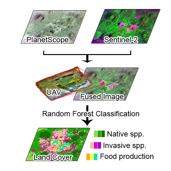
In this paper, we presented a replicable methodology that uses free and open-source data to monitor land use and land cover change in complex agricultural systems. Agricultural landscapes are a complex patchwork of food crops and other vegetation types, where even small-scale patches of vegetation can be a valuable habitat for animals of different kinds [82,83,84,85,86]. Having images with high spatial resolution is crucial for capturing small habitat fragments in the analysis, so methods that use freely-available high-resolution image collections provide a much-needed and inexpensive alternative to purchasing commercial high-resolution data for fine-scale analysis. Mapping an agricultural matrix in high resolution is a challenge because categorically different vegetation types can have similar spectral signatures and be cultivated in proximity with other vegetation types; our object-oriented random forest classification of fused images tackles this challenge by combining data sources with complementing resolutions, taking into account the geometrical properties of landscape features in addition to their reflectance, and by classifying elements with an algorithm that provides reliable results with limited training datasets [24,27].

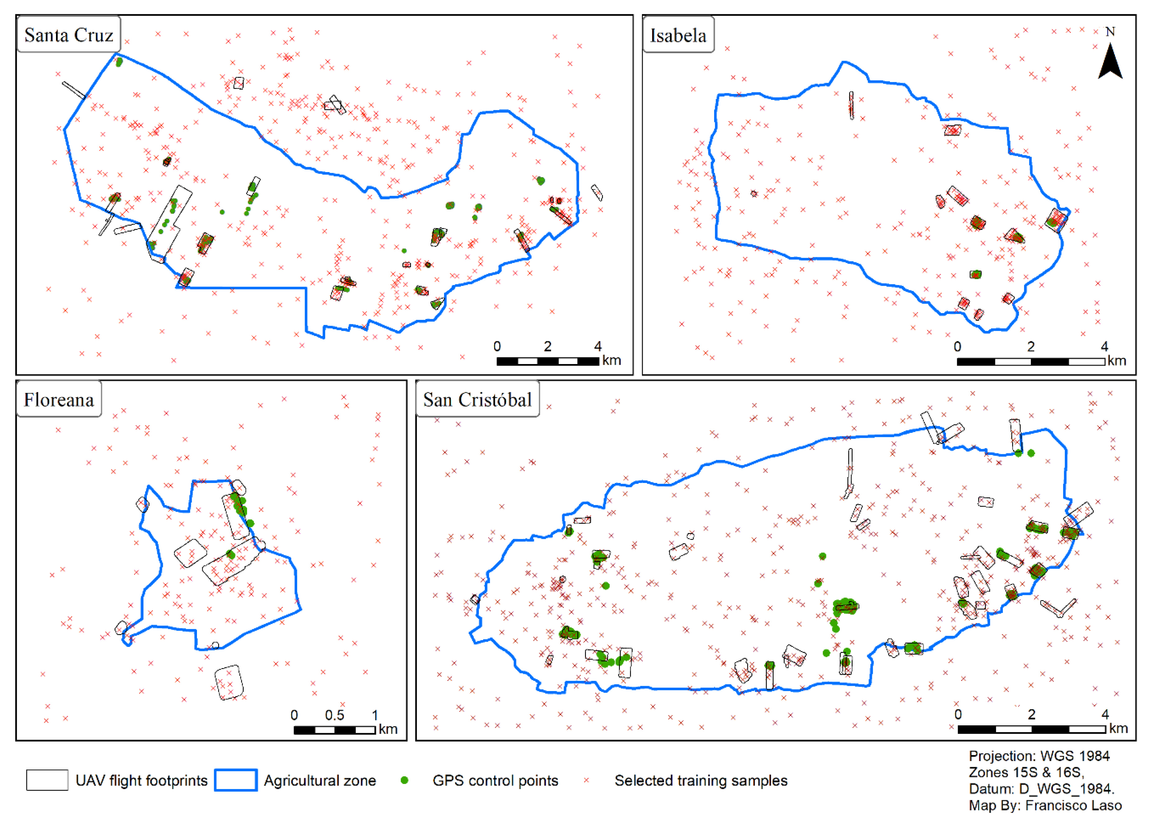
Unfortunately, two land cover types, Lantana and Erythrina, had to be dropped from the final mapping outcomes because we did not have enough reference points to have consistent results during classification. In the case of Erythrina, their proximity to other dense vegetation types, such as permanent crops, Cedrela, and Psidium, was an issue during segmentation. Erythrina trees are usually planted in long stands as living fences are often pruned, so their crowns tend to be relatively small. Therefore, the size of Erythrina stands was insufficient to be adequately captured by the sensors, even at 3 m resolution. The small size and proximity to other vegetation types caused segments to include neighboring pixels of different land cover types and confuse their spectral signatures. Similarly, in the case of Lantana, we did not have enough examples of patches that were large enough to produce a clear spectral response. Additionally, we were limited in our reference data available because some areas lacking information were too remote or of difficult access to reach them by foot to collect GPS control points. On the other hand, weather conditions in the highlands also made image collection with a UAV difficult and sometimes impossible within the timeframe available for fieldwork, as was the case with Isabela’s highest regions within our study area. Therefore, areas that were easier to access or had favorable weather conditions were more represented in our samples.

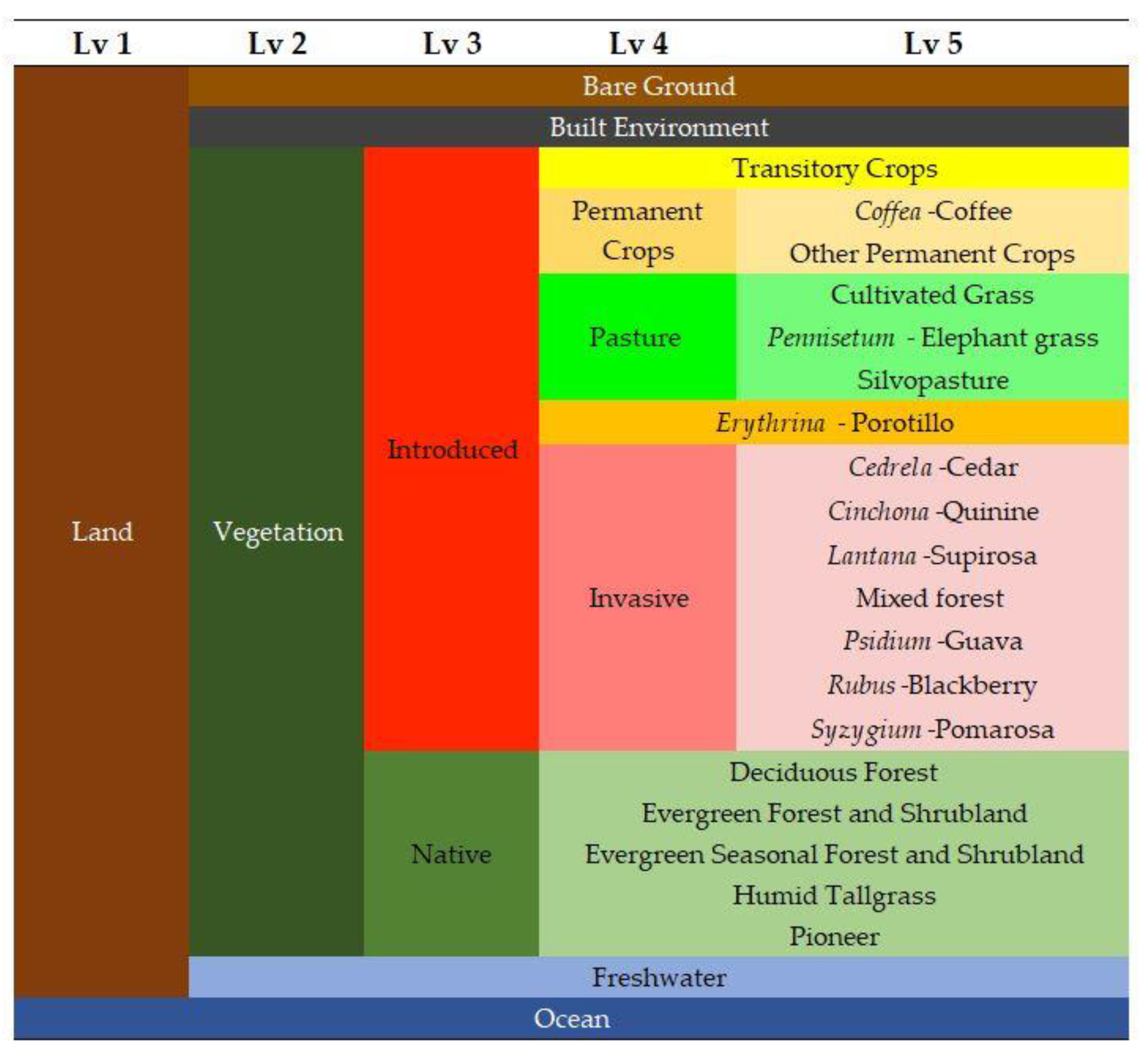
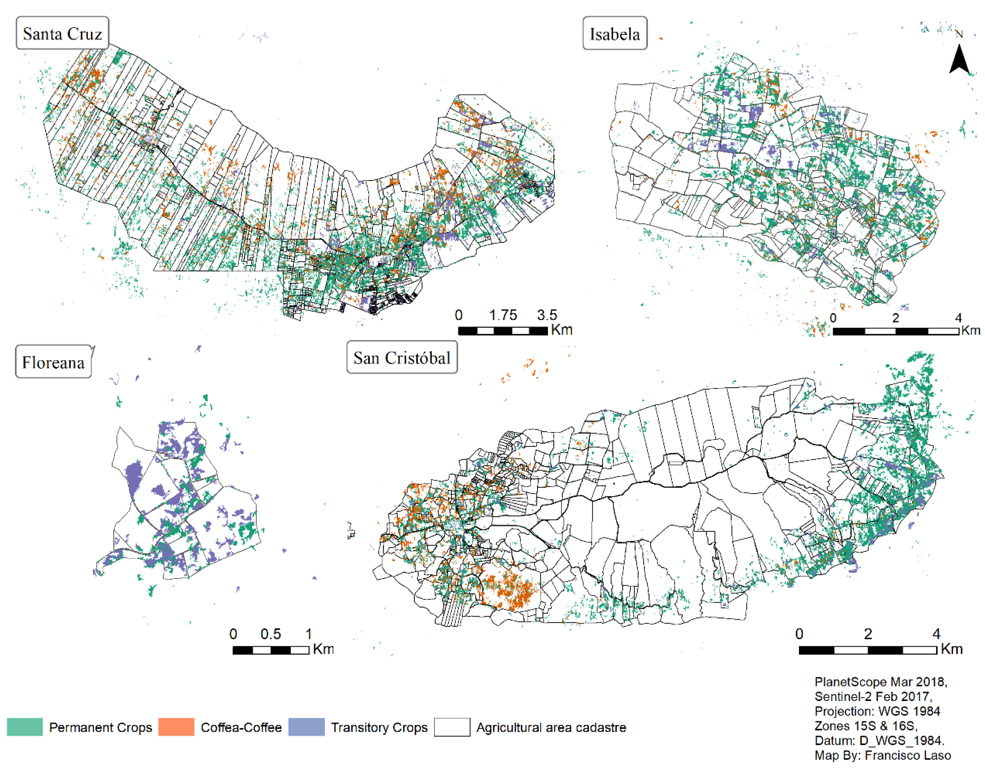
Additionally, land cover units grouping several species, instead of mapping individual plants, were adopted because these types of general categories are used in policy documents or previous studies. While this makes our results relevant to the intended users of the map (i.e., MAG) and compatible with existing data sources, these categories forced us to group together vegetation types into land cover units that likely had a wide range of spectral signatures. For example, permanent crops, transitory crops, silvopastures, and mixed forest are land cover units that are heterogeneous by definition. For instance, permanent crops are often tree crops, but MAG also includes pineapples in this category since they are technically perennial crops [40]. Pineapple plantations have a very different spectral signature than tree stands. This inclusion might explain why permanent crops were the most frequently misclassified category (error rate = 28% in Santa Cruz, Table 9). Similarly, silvopastures are, by definition, a mixture of grass and tree species, both of which could be of different types and have vastly different reflectance, and this probably contributed to their misclassification and high error rate (error rate = 38% in Santa Cruz, Table 9). Likewise, the mixed forest is defined as an area where invasive species co-dominate with native species [42]. Given there is a wide range of species, both native and introduced, that could fit that description, it is understandable that humans and computer algorithms could easily misclassify these areas (error rate = 12% in Cristobal and Floreana, Table 9).

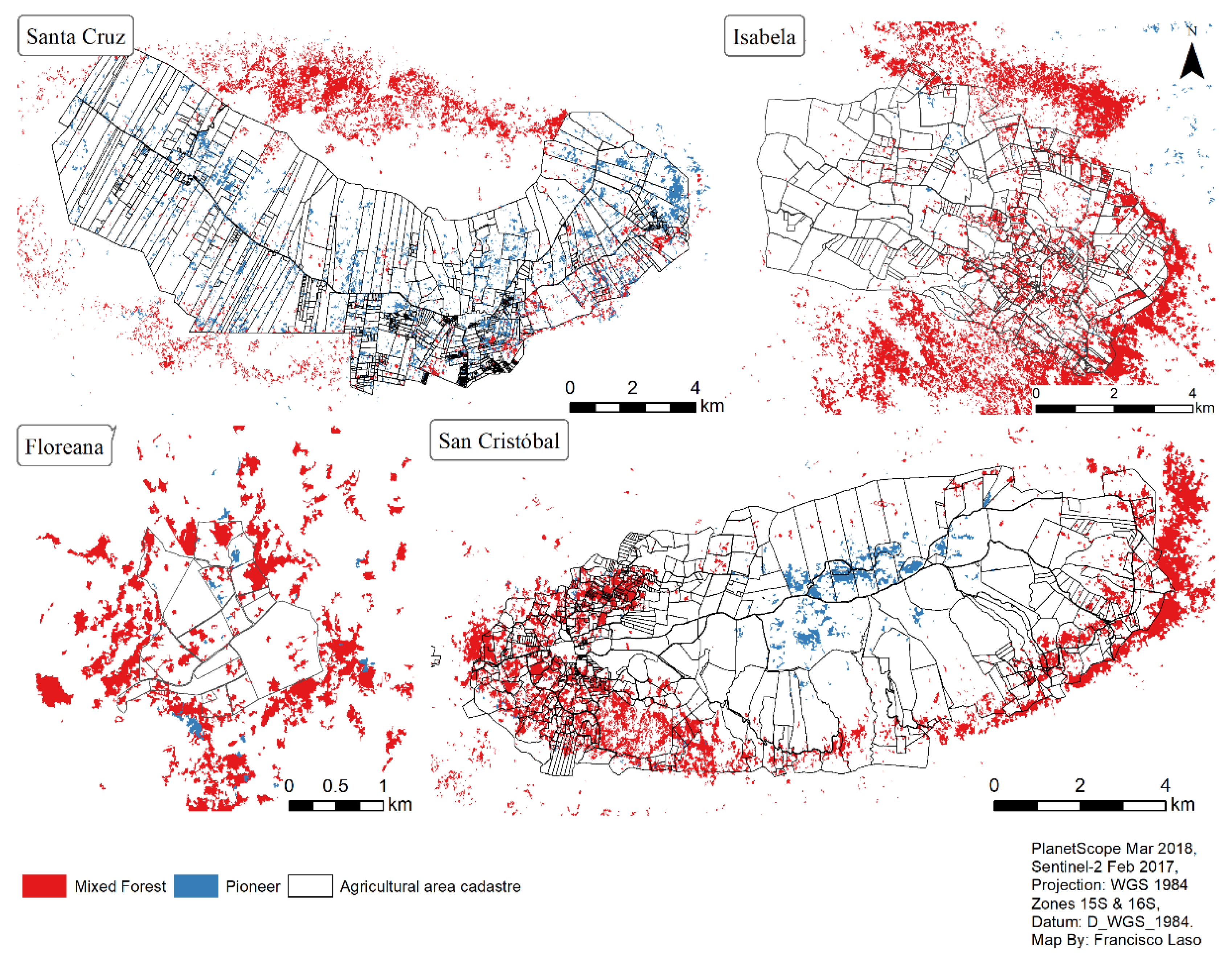
Another challenge to mapping the agricultural area is that this is a very dynamic landscape, and its land cover is always changing. For example, both transitory crops and pioneer vegetation are, by definition, short-lived; farmers harvest transitory crops in less than one year, and succession quickly leads other plants to take over disturbed areas where pioneer plants once thrived. This short life probably confused their classification because the spectral life of specific land cover types is shorter than the two-year timeframe when the different satellite images were collected. Short spectral life might be one of the main reasons why the ‘pioneer’ land cover unit received the lowest R² score (0.032) during map validation. Despite their ephemeral nature, it was important to include these categories to remain consistent with other data sources and to try to capture a snapshot of current vegetation cover. Furthermore, temporary vegetation covers like ‘pioneer’ or heterogeneous categories like ‘mixed forest’ might signal that these areas are currently in flux, so their presence helps represent the dynamic nature of the agricultural areas.

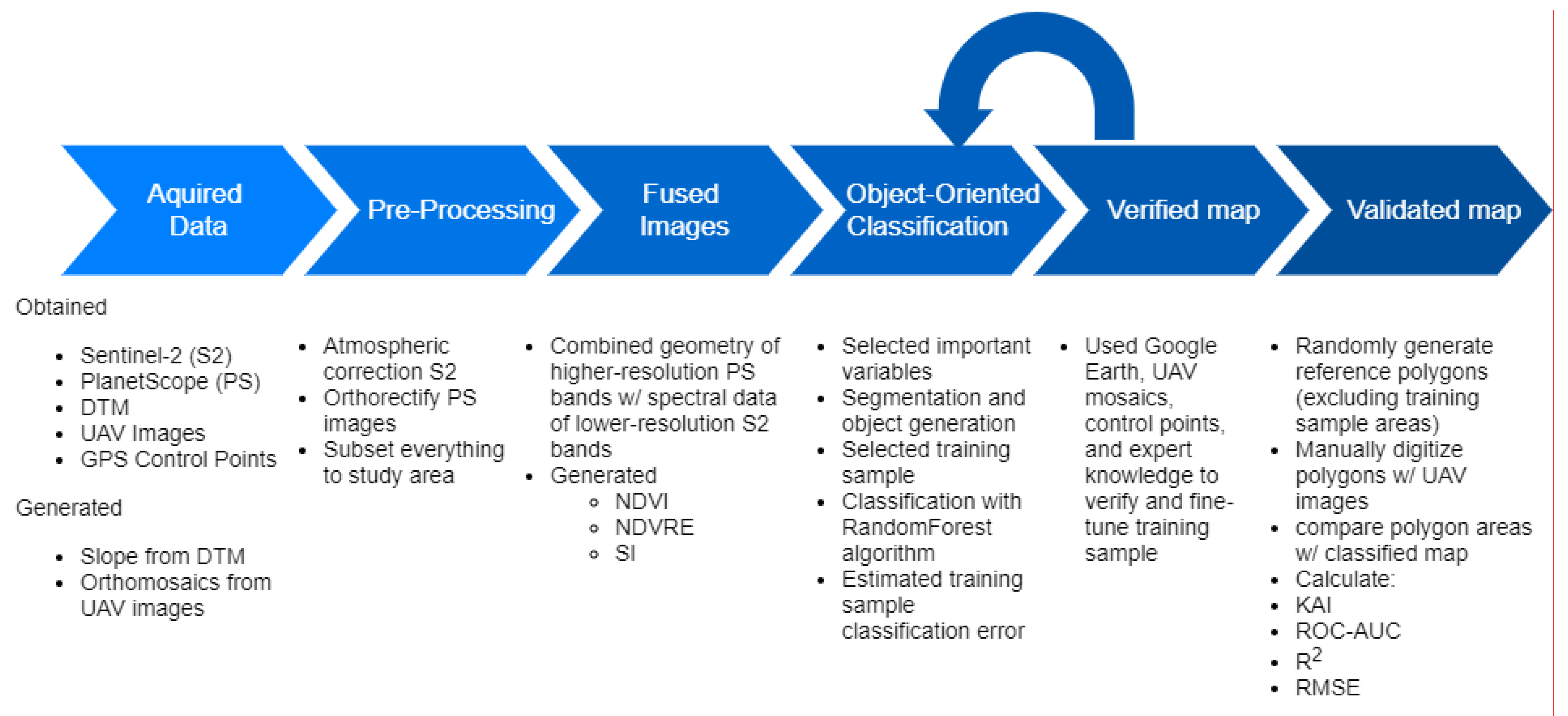
The landscape and the classification units themselves are not homogenous, so traditional methods for assessing accuracy are limited by the assumption that each area in the map can be unambiguously assigned to a single category, and by expressing classification errors as either “right” or “wrong” without reference to the magnitude of the error [87]. We initially attempted a point-based accuracy assessment, but this yielded misleadingly low results because GPS control points of individual plant species could not be unequivocally assigned to any one category. Therefore, we opted for a validation method that could accommodate for the landscape’s and our classification scheme’s ambiguity. Expressing our accuracy in terms of percentages and correlations RMSE and R² was more relevant to the users of our classification because we are comparing manually-classified reference polygons with our classification results. However, we included other metrics common in land cover classification and machine learning (KIA, AUC) to reach readers that are more accustomed to them.

Our accuracy assessment results are in a similar range as those from similar object-based land cover classifications [24,69]. Our overall KIA value of 0.7 suggests that our classification results are significant and are useful overall. Categories with KIA or AUC values >0.7 correspond to land cover types with a forest or pasture structure (Table A5). The land covers that were confused most often were bare ground, freshwater, and pioneer cover types. (Table A5). All three land cover types covered relatively small surface area extensions, so their representation in the validation reference polygons was minimal. This error was especially strong for freshwater (KIA: 0.34, AUC: 0.314) because most visible freshwater occurs in microreservoirs, for which reflectance can change drastically depending on whether or not they are filled. Only one microreservoir fell within the reference polygons for classification. Bare ground (KIA: 0.271, AUC: 0.386) was understandably confused with transitory crops (KIA: 0.446, AUC 0.628) because these areas are usually denuded from other vegetation, and so the spectral response of the bare soil gets confused with that of the crops themselves. Bare ground is also hard to distinguish from built environment (KIA: 0.516, AUC: 0.685) because most roads of the humid highlands remain dirt roads and are not paved yet. Pioneer land cover (KIA: 0.22, AUC: 0.31) was probably confused with several other categories due to their ephemeral nature, as described above. Of the four categories with an AUC value between 0.6 and 0.7, two correspond to land cover types that grow below the forest canopy, such as Coffea (KIA: 1.927, AUC: 0.676) and Rubus (KIA:0.417, AUC: 0.603), so it makes sense that their AUC values are not as high, as their spectral signatures can become confused with other vegetation types. The other two categories with an AUC between 0.6 and 0.7 are built environments and transitory crops, which, as mentioned earlier, both become confused with bare ground.

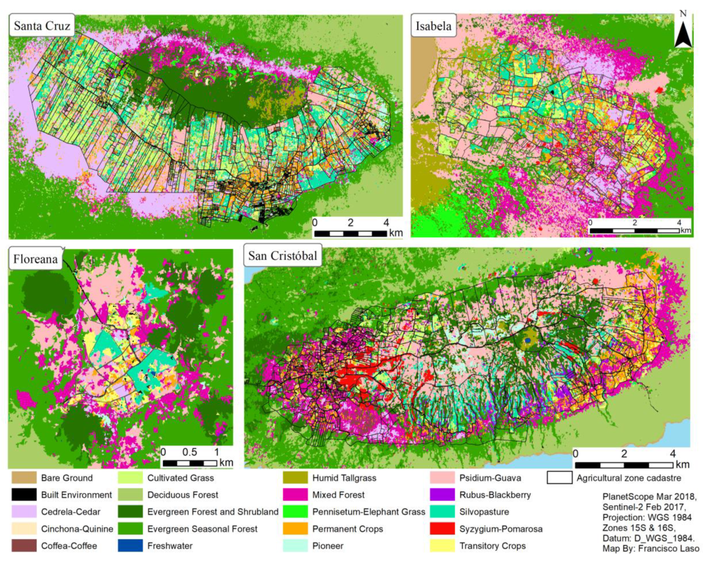
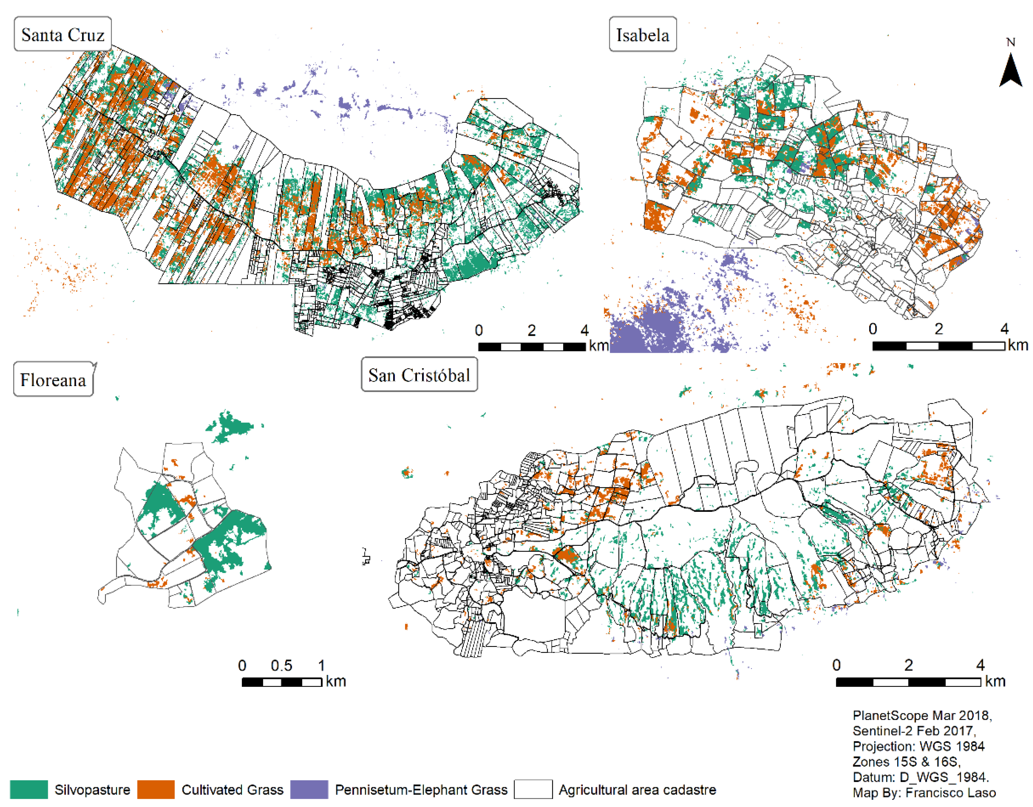
Our results suggest that our classification map likely represents general patterns (large patches) relatively well, especially for categories that had a clear spectral signature and, thus, had a high correlation coefficient as well, such as Cedrela, Pennisetum, and Syzygium. However, the landscape’s heterogeneity means that the map likely becomes more inaccurate as one approaches smaller scales. The fact that the two largest islands, Santa Cruz and San Cristobal, had the highest R² values (0.83 and 0.7, respectively) might be due to these islands having larger farms with a more regular and well-delimited configuration of their crops than smaller farms from Isabela or Floreana.

While human digitation using high-resolution UAV images would usually have more accurate results than using segments mapped by a computer, the fact that we are using satellite images with a 3 m spatial resolution means that we are within the margin of error for most GPS devices, including our drone. This might cause misalignment with the high-resolution images that we used to obtain the geometry for the reference polygons, thus lowering our accuracy results. Furthermore, given that we used the most homogenous land cover patches visible within our UAV images to help us pick areas to train the algorithm, remaining unused areas of our images were also the most mixed and harder to categorize, which might have affected our accuracy scores as well.

4.2. Vegetation Cover Abundance and Distribution

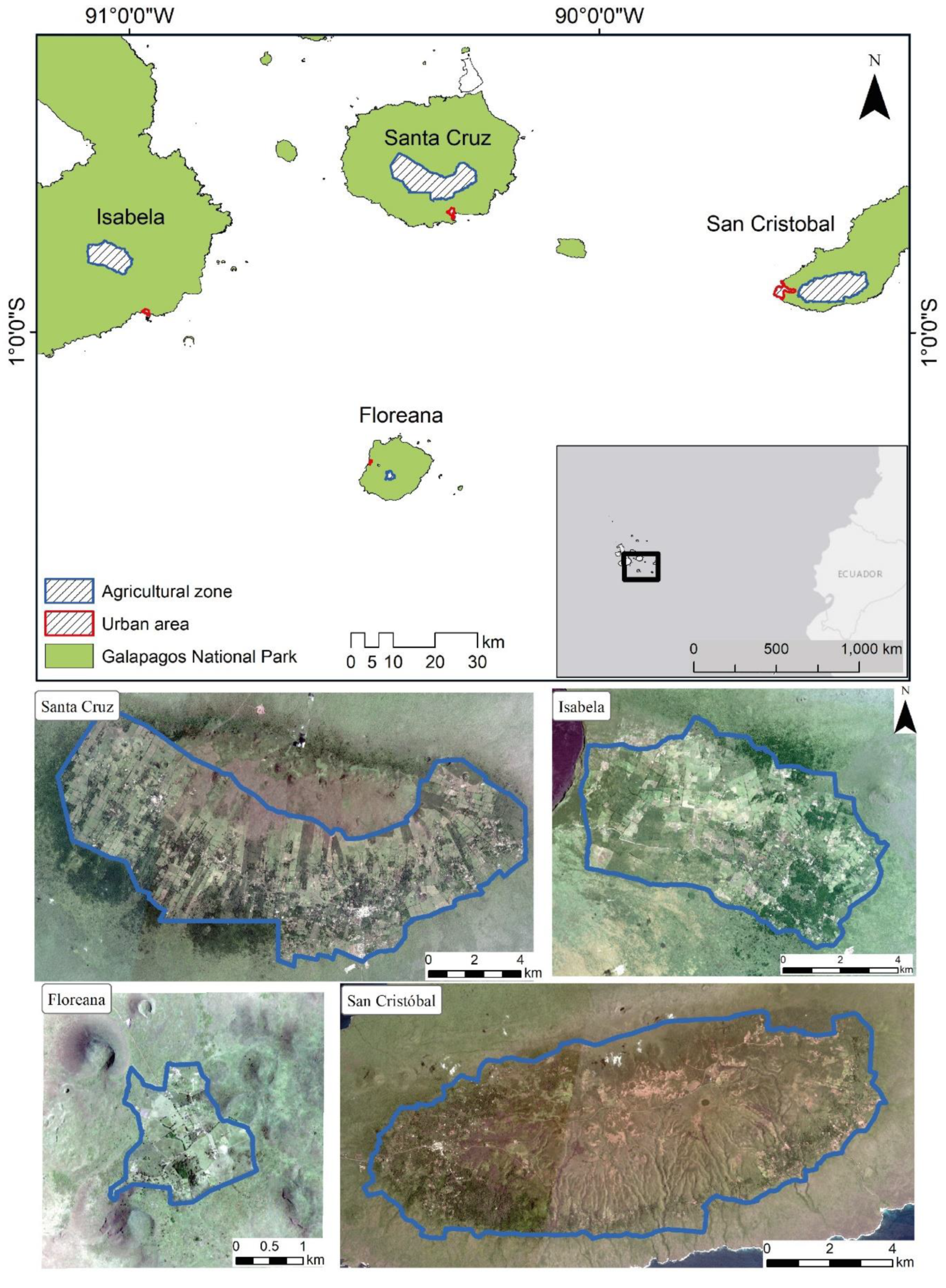
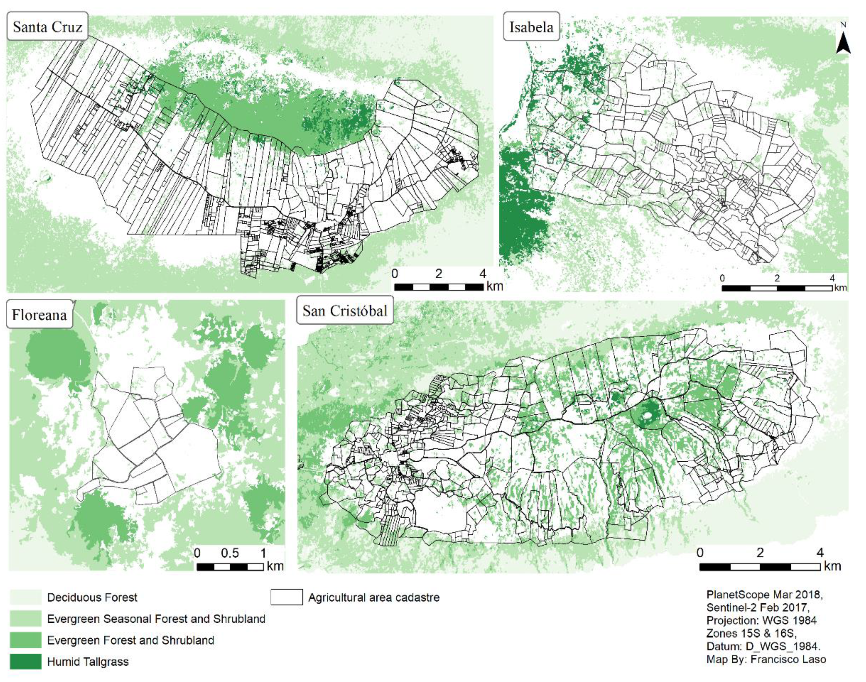
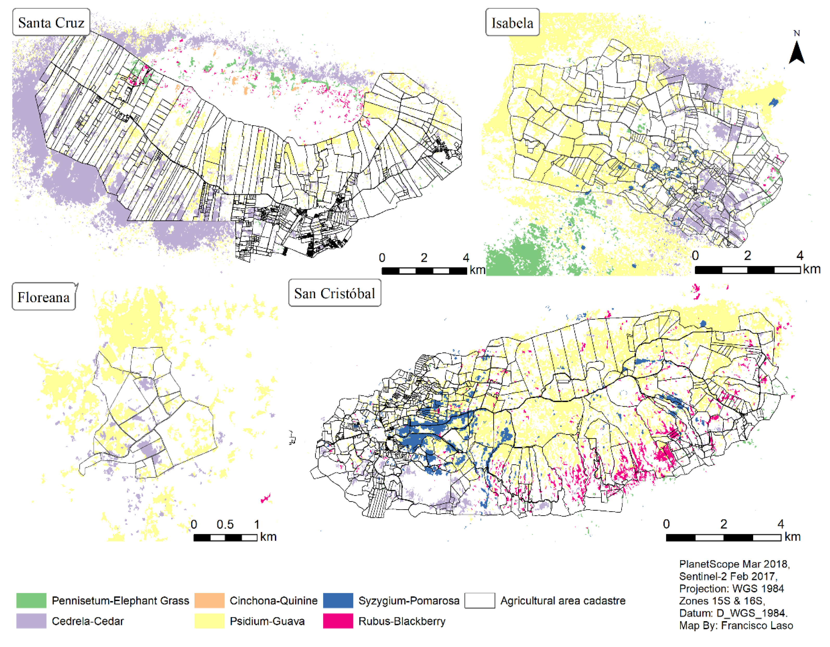
The fact that the areas surrounding the agricultural areas are GNP lands under conservation means that we expected to find a difference in the vegetation covers within and outside the agricultural areas. As expected, we found that most native vegetation is distributed outside the agricultural zone while invasive species dominate the area within the agricultural areas (Figure A1 and Figure A2). However, we also expected to see this pattern due to the long history of agricultural exploitation within the Galapagos. The most aggressive agricultural expansion occurred in San Cristobal from 1879 to 1904 under the rule of Manuel J. Cobos, and this set the tone for commercial development of agriculture in other islands as well. During this time the highlands of San Cristobal were denuded of native vegetation, P. guajava and avocado trees were brought for pig food, Sygzygium trees were imported to provide shade for wool sheep, pastures were introduced for extensive cattle grazing to sell cowhides, up to 3000 ha of sugar cane were planted for sugar and liqueur production and export, and over 100,000 coffee plants covered 110 ha of plantation [88]. In comparison, today, all food crops found in our study area combined barely cover a third of the area that was once covered by sugar cane alone. San Cristobal has the most substantial extensions of Sygzygium trees in the entire archipelago (374 ha), and P. guajava covers 23% of the agricultural area. While agricultural activity as a whole has become a fraction of what the island once supported, the area covered by coffee plantations has increased to 191 ha. Given the level of agricultural exploitation, perhaps what is surprising is that San Cristobal also shows the most amount of native vegetation within its agricultural area, which is likely due in part to the work of the GNP reforesting the areas around El Junco with Miconia robinsoniana.

Other islands followed similar patterns but at different times. Floreana’s first successful inhabitants took residence in the 1930s, and they subsisted by modifying the highlands by knocking down trees, clearing the land, hunting wild cattle, and introducing seeds for crops. For example, the Cruz family, who arrived to Floreana in 1937, dedicated their time to agricultural production and cattle ranching. As their family grew, so did their land and the pastures that covered them; because the population was so small (55 people by 1975), life in Floreana was only assured through agricultural production. By 1965, farmers planted entire hectares of individual transitory crops year-round, and they harvested the fruit from citrus trees that grew wild inside and outside of the agricultural areas [88]. These patterns are visible in our results, as there are large areas of land dedicated to cattle production and mixed forest surrounds the agricultural area. We also see evidence of more recent events, such as the spread of R. niveus and P. guajava across the landscape [88].

In Isabela, there was a 900 ha farm called “La Hacienda” that was established in 1897 by Carlos Gil Quezada. Quezada’s main economic activity was cattle ranching, and through the 1950s, he captured wild cattle that roamed the pampas of Sierra Negra volcano and exported them to Guayaquil [88,89]. Given that La Hacienda is reported to be relatively near the southeastern border of the present-day agricultural zone, it is entirely possible that the pastures visible to the southwest of the agricultural area are the same areas that were used as cattle hunting grounds by Gil Quezada. It would seem unusual that pastures are found outside of the agricultural zone, and the species found in those grasslands remain unconfirmed. We do not have direct verification of the vegetation of this site, but the spectral signature of this region is distinct, and during the development of the land cover map of the GNP [42], park rangers indicated to the authors that these are Pennisetum grasslands, so we categorized this region in the same manner. The observed large expansions of invasive species in Isabela are consistent with the recorded process of extensive cattle grazing and subsequent abandoning of lands since the 1980s as meat production became less profitable, leaving Isabela’s last remaining stronghold of agricultural production concentrated in the lowest (easternmost) section of the agricultural zone [88], which is the same region where transitory and permanent crops can be seen today.

The prevalence of pastures in the agricultural area of Santa Cruz is well reported [40,90,91] and is consistent with our results. The presence of Cedrela odorata stands in GNP lands (but barely in the agricultural area) makes sense because, since its intentional introduction in the 1940s, the Ministry of the Environment prohibited the exploitation of Cedrela in 2007 due to its threatened status in the continental area. However, by 2009, it allowed the extraction of C. odorata once again, but only within the agricultural zone [92]. The distribution of P. guajava in Santa Cruz is also consistent with our current understanding of how cattle and tortoises are dispersing this invasive plant [51], and the presence of other invasive plants like R. niveus was also expected in all four inhabited islands [93]. It should be noted that plant species like R. niveus and Coffea commonly grow in the understory of a vegetated area. When trying to capture vegetation that lies in the understory, the spectral signal becomes mixed with that of the tree canopy, so ours is an underestimate of the true extent of these vegetation types.

4.3. Comparing and Combining Results with Existing Datasets

Given that this is the first study to map the agricultural areas in high-resolution, we can compare our results with self-reported surface areas of the agricultural zone from the 2014 agricultural census [40].

Table 14. Results comparison between the 2014 Agricultural Census and this study. The left section of the table summarizes the results from the 2014 Agricultural Census and the right side of the table groups land cover types of this study to make them comparable with the agricultural census.

2014 Agricultural Census			This Study
Land Cover / Use	ha	%	ha	%	Categories Included
Permanent crops	1517	8	3913	15	Permanent Crops, Coffea
Transitory crops	220	1	698	3	Transitory crops
Tilled land	110	1	NA	NA
Fallow land	433	2	NA	NA
Pastures	11,126	59	5618	22	Cultivated Grass, Pennisetum, Silvopasture
Invasive species	934	5	7080	28	Psidium, Rubus, Cinchona, Syzygium, Cedrela
Pioneer and forest	4189	22	7630	30	Pioneer, Mixed Forest, Native vegetation
Other Uses	482	3	307	1	Built Environment, bare ground, water
Total	19,010	100	25,246	100

lists the main categories used by the agricultural census on the left and the corresponding categories of this study to the right. We would expect to see discrepancies between the results for several reasons: the agricultural census does not encompass all producers, but rather a sample of 755 of the most productive and representative ones, whereas our study encompasses the entirety of the agricultural area. Therefore, our estimated land covers might include areas that are not tended by anyone. This might account for dramatic increases in reported permanent crops, for example, as many fruit trees within the agricultural area might simply be growing wild, and respondents might not have taken them into account for their responses. Furthermore, both sources have their own inaccuracies: while our study is susceptible to misclassifications, self-reported values may be susceptible to under or over-estimating surface areas. This might be the case for Transitory crops, where our classification might easily categorize ‘tilled land’ and possibly even fallow land as transitory crops. Perhaps not coincidentally, the two values become very similar if tilled and fallow lands are included in the estimate. Furthermore, respondents to the census may have different definitions of what falls within each category. For example, some farmers might not consider P. guajava an invasive plant, as they might see it as an important element of their silvopastures. This is the reason why, for Table 14, we categorized Pennisetum as a pasture and excluded it from the invasive category because farmers use this grass species for their cattle and would likely not consider it ‘invasive’. Furthermore, the category “Pioneer and forest species” is a category that encompasses any vegetation that has no agricultural value for farmers, so it is very general.

Despite the many ways in which these data might not match, the dramatic decrease in pastures and the astounding increase in invasive plants across all four islands are probably real trends. This would be consistent with the observed trend of decreasing pastures between the 2000 census (14,555 ha) and the 2014 census (11,126 ha) [41]. This would also be consistent with the fact that the region’s worst-recorded drought occurred in 2016, which MAG officials reported drove many cattle ranchers to abandon this activity as many cattle died due to the dry conditions [personal communication]. A drop in pastures, combined with an increase in invasives, is exactly what we would expect from people abandoning their lands. Pastures have a spectral signature that is very different from other land cover types, so it is unlikely that they were so heavily misclassified. However, it is possible that even though we grouped silvopastures as part of our estimate for pastures, farmers might still identify more heavily wooded areas as “pastures” while our algorithm might have identified the same region as a forest of some type. Lastly, although it is hard to compare specific numbers due to differences in methodologies and missing information, authors did find a general decrease of pastures in the agricultural areas and an increase in invasive plants in Santa Cruz and San Cristobal from 1987 to 2006 [90]. The present study serves as much needed baseline data with a replicable methodology that can complement existing studies [42] to give us, for the first time, a truly complete view of land cover for the entire archipelago (Appendix C,

Table A6. Total area occupied by each of the categories and land cover classes for the entire Galapagos province.*

Category	Land Cover Classes	Protected Area [35]	Agricultural Area	Total	%
Forest and Shrub	Evergreen forest and shrubland	30,788.9	2425.8	33,214.7	4.2
	Evergreen seasonal forest and shrubland	60,887.7	1640.9	62,528.6	7.9
	Coastal humid forest and shrubland	1377.5		1377.5	0.2
	Deciduous forest	262,527	268.8	262,795.8	33.0
	Deciduous shrubland	28,258		28,258.0	3.5
Herbaceuos vegetation	Humid Tallgrass	4477.5	369.7	4847.2	0.6
	Highland deciduous tallgrass	6922.6		6922.6	0.9
	Deciduous tallgrass	17,137.4		17,137.4	2.2
Mangroves	Mangrove forest	1470.4		1470.4	0.2
Invasive Species	Cedrela—cedar	1977.4	1349.4	3326.8	0.4
	Mixed	1142.1	1875.4	3017.5	0.4
	Rubus—blackberry	495.1	324.8	819.9	0.1
	Pennisetum—grass	2871.7	103.8	2975.5	0.4
	Cinchona—quinine	61	17.4	78.4	0.0
	Psidium—guava	10,312.6	4955.2	15,267.8	1.9
	Syzygium—Pomarrosa		433.4	433.4	0.1
Rocky outcrop	Recent lavas	252,273.3		252,273.3	31.7
	Old lavas	87,914.8	18.6	87,933.4	11.0
Agricultural Areas	Coffea—Coffee		944.5	944.5	0.1
	Cultivated Grass		2402.0	2402.0	0.3
	Silvopastures		3112.9	3112.9	0.4
	Transitory Crops		698.2	698.2	0.1
	Permanent Crops		2968.1	2968.1	0.4
Other	Urban settings	550.7	258.8	809.5	0.1
	Water	705.7	29.4	735.1	0.1
Total		772,151.4	24,197.17	796,348.6	100

*Note: Shaded cells group together individual land cover classes into general categories.

).

4.4. Broader Significance

Our methods and our findings are relevant to complex agricultural landscapes in general and in ongoing conversations about conservation and food security, particularly in the context of other oceanic islands, as well as ‘islands’ of protected forests within an agricultural matrix. Our replicable methods are useful to map other islands, other agricultural landscapes, and other time periods beyond the ones presented here.

The fact that the agricultural sector has been neglected, especially in comparison to more robust economic sectors like tourism, development, or conservation, is not unique to the Galapagos. There is a global trend of abandonment of the agricultural sector and a migration of rural population into urban centers [94,95]. Furthermore, oceanic islands worldwide are typical tourism hotspots and suffer from similar pressures as does the Galapagos: reduced space for food production and an overdependence on food imports to sustain their human populations [96,97,98]. Our results are relevant in the context of global food security and particularly in food security on islands because of familiar socioeconomic and environmental drivers of pattern in island ecosystems [98,99]. Baseline data such as that provided in this study is essential to track changes in land use and land cover in our food systems and to anticipate the ways in which climate change can make them more vulnerable to collapse, as well as to help us identify the land uses and land covers that are most resilient to environmental change [99,100].

The vast extent of pastures found in our study should prompt decision-makers to reconsider whether this land use is the most sound in a place where the space to grow food is so limited. Our study confirms that soil depth and precipitation patterns in this region can support an astounding diversity of permanent and transitory crops, and pasture monocultures to feed cattle might not efficiently support local food security. It is relevant that decisionmakers of the Galapagos have promoted silvopastoral systems as a more sustainable alternative to pasture monocultures. Given that most pastures and silvopastures of the Galapagos are grain-fed, having an estimate of the distribution of silvopastoral systems allows us to compare their performance in the context of more variable and extreme seasonality.

Our results are also relevant in the conversations about novel ecosystems and island biogeography. Our focus on native ecosystems and invasive species make our results applicable to other island ecosystems because the biogeographical features of oceanic islands lead to high endemism rates and simultaneously make them more susceptible to invasion from introduced species [101]. In addition, there is a clear spatial correlation between human activities and invasive species, even long after these activities were abandoned [1,102]. For example, even though San Cristobal has not had sheep raised for wool in recent history, the fact that Manuel Cobos once used Syzygium on this island to give shade to sheep [88] is likely the reason why over a hundred years later Syzygium remains concentrated on San Cristobal rather than in other islands. Human agency profoundly modifies the agricultural landscape and its surrounding areas, and our results support previous observations that introduced species can become integrated into native landscapes, perhaps irreversibly [38,103]. For example, the extent of colonization by Psidium guajava or Rubus niveus pose a particular challenge for conservation projects that would like to see protected areas returned to a pre-human state. These plants now serve as an essential food source for endemic fauna like finches and tortoises and, thus, have become profoundly integrated into the life cycles of the emblematic species who disperse the seeds across their habitat [51,104,105,106]. Our results show examples of what previous authors have called novel ecosystems in which humans have crossed some ecological thresholds that gave rise to a historically new and stable species assemblage [107]. However, our results also demonstrate the capacity of human agency to modify the environment in the face of highly aggressive invasive plants. For example, Cedrela odorata’s distribution in Santa Cruz and the prevalence of native ecosystems within the agricultural area of San Cristobal both suggest that the work of private landowners and the GNP can be effective at controlling the spread of invasive plants and propagating the land cover of our choosing.

4.5. Next Steps

We envision that one of the potential next steps following this baseline map of the highlands of the Galapagos would be the use of additional vegetation indices to recategorize existing land covers with greater detail. New and more specific categories must be created to tease apart the differences in general categories, such as the current ‘mixed forest,’ ‘permanent crops,’ or transitory crops’. It is also advisable that future iterations of land cover maps be able to distinguish introduced plants like Lantana and Erythrina.

5. Conclusions

In this paper, we have presented a replicable and reliable methodology for land cover classification combining freely-available high-resolution data sources and taking advantage of their complementing spectral and spatial resolutions. The methods described are well suited to classify complex agricultural landscapes by taking into account the geometry of scene elements in addition to their reflectance.

We found that our spatial resolution was insufficient to reliably detect rows of living fences of Erythrina since their crown size was often less than the 3 m pixel size of our data sources. However, our methods were able to reliably identify stands of invasive plants like C. odorata, S. jambos, and P. guajava. Our results suggest that out of the 25,261 ha of the agricultural zone, invasive plants cover most of the surface area (28%), mostly dominated by P. guajava (4959 ha). Pastures for raising cattle cover 22% of the agricultural zones, the majority of which are located in Santa Cruz. Most native vegetation is distributed outside of the agricultural areas, but almost 19% of the agricultural zone’s land cover was identified as native vegetation, mainly located in San Cristobal (2535 ha). Food crops of different kinds cumulatively cover a similar percentage (18%) of the surface area, and about 944 ha of these are dedicated to coffee cultivation, mostly located in Santa Cruz. About 12% of the agricultural sector is covered by vegetation that could not be clearly identified as either native or invasive vegetation.

Multiple institutions and researchers have expressed the need for a high-resolution and updated and land cover classification of Galapagos agroecosystems. Local agencies in the agricultural sector can now use these data for identifying current agricultural resources and planning land management projects. For example, the classification maps will inform the GNP and the MAG about priority areas for intervention to control invasive species; having clear estimates of surface area covered by different invasive plants allows institutions to make realistic estimates of approximate costs for their control as part of long-term plans for the region. Authorities can now ascertain the trends of the region’s food basket with greater confidence, to ascertain whether food crops and pastures have increased or diminished in relation to previous years as well as in relation to future assessments. These data help local authorities plan strategic interventions, such as estimating how many people are necessary to make the most of land that is already being planted, as well as how many people would be necessary to reactivate areas currently dominated by invasive plants. Additionally, researchers can use these baseline data to anticipate changes in land cover as socioeconomic and environmental drivers continue to change observed land use and climate patterns. The land cover categorization and mapping strategy is designed to be reproducible so that it can be applied to future images to track changes in these agroecosystems.

The dataset presented here is designed to suit the needs of both agricultural and conservation practitioners. We aim to encourage collaboration between these two sectors to ensure the well-being of Galapagos inhabitants and the sustainable preservation of its ecosystems and to serve as a model for land use mapping in other environments globally where agroecosystems host essential species for conservation.

References

1. Hobbs, R.J.; Arico, S.; Aronson, J.; Baron, J.S.; Bridgewater, P.; Cramer, V.A.; Epstein, P.R.; Ewel, J.J.; Klink, C.A.; Lugo, A.E.; et al. Novel ecosystems: Theoretical and management aspects of the new ecological world order. Glob. Ecol. Biogeogr. 2006, 15, 1–7. [Google Scholar] [CrossRef]
2. McCleary, A.L. Characterizing Contemporary Land Use/Cover Change on Isabela Island, Galápagos. In Science and Conservation in the Galapagos Islands: Frameworks and Perspectives; Walsh, S., Mena, C., Eds.; Springer: Berlin/Heidelberg, Germany, 2013; Volume 1, pp. 155–172. ISBN 978-1-4614-5793-0. [Google Scholar]
3. Guézou, A.; Trueman, M.; Buddenhagen, C.E.; Chamorro, S.; Guerrero, A.M.; Pozo, P.; Atkinson, R. An extensive alien plant inventory from the inhabited areas of galapagos. PLoS ONE 2010, 5, 1–8. [Google Scholar] [CrossRef] [PubMed] [Green Version]
4. Chiriboga, R.; Maignan, S.; Fonseca, B. Producto 2: Caracterización de Los Sistemas de Producción en Galapagos en Relación con el Fenómeno de las Especies Invasoras; Technical Report: Proyecto ECU/00/G31” Control de las especies invasoras en el Archipielago de Galapagos”; United Nations Development Programme (UNDP): Galapagos, Ecuador, 2006. [Google Scholar]
5. Valdivia, G.; Wolford, W.; Polo, P.; Pena, K.; Nelson, J.; Perry, S.; Lu, H.; Hansanungrum, N.; Walsh-Dilley, M. Supporting Local Food Systems: New Geographies of Conservation and Production in Galápagos; Technical Report; Cornell University Student Multidisciplinary Applied Research Team (SMART): Galapagos, Ecuador, 2013. [Google Scholar]
6. Ministerio de Agricultura, Ganaderia, Aquacultura, y Pesca; Ministerio del Medio Ambiente del Ecuador. Plan de Bioagricultura para Galápagos Una Oportunidad para el buen Vivir Insular-Resumen Ejecutivo, 2014.
7. Toledo, A. Rentabilidad de la Producción Agrícola en Santa Cruz, Galápagos; Technical Report; Conservation International: Galapagos, Ecuador, 2014. [Google Scholar]
8. Blake, S.; Yackulic, C.B.; Cabrera, F.; Tapia, W.; Gibbs, J.P.; Kümmeth, F.; Wikelski, M. Vegetation dynamics drive segregation by body size in Galapagos tortoises migrating across altitudinal gradients. J. Anim. Ecol. 2013, 82, 310–321. [Google Scholar] [CrossRef] [PubMed] [Green Version]
9. Dvorak, M.; Fessl, B.; Nemeth, E.; Kleindorfer, S.; Tebbich, S. Distribution and abundance of Darwin’s finches and other land birds on Santa Cruz Island, Galápagos: Evidence for declining populations. Oryx 2012, 46, 78–86. [Google Scholar] [CrossRef] [Green Version]
10. Blake, S.; Guezou, A.; Deem, S.L.; Yackulic, C.B.; Cabrera, F. The Dominance of Introduced Plant Species in the Diets of Migratory Galapagos Tortoises Increases with Elevation on a Human-Occupied Island. Biotropica 2015, 47, 246–258. [Google Scholar] [CrossRef]
11. Benitez-Capistros, F.; Camperio, G.; Hugé, J.; Dahdouh-Guebas, F.; Koedam, N. Emergent conservation conflicts in the galapagos islands: Human-giant tortoise interactions in the rural area of santa cruz island. PLoS ONE 2018, 13, e0202268. [Google Scholar] [CrossRef] [Green Version]
12. Blake, S.; Yackulic, C.B.; Wikelski, M.; Gibbs, J.P.; Deem, S.; Villamar, F. La migración de las tortugas gigantes de Galápagos requiere de esfuerzos de conservación a escala de paisaje. In Informe Galapagos 2013–2014; Galapagos National Park, Consejo de Gobierno del Regimen Especial de Galapagos, Fundacion Charles Darwin, Galapagos Conservancy: Puerto Ayora, Galapagos, Ecuador, 2014. [Google Scholar]
13. Liaghat, S.; Balasundram, S.K. A Review: The Role of Remote Sensing in Precision Agriculture. Agriculture 2010, 5, 50–55. [Google Scholar] [CrossRef] [Green Version]
14. Green, E.P.; Mumby, P.J.; Edwards, A.J.; Clark, C.D. A review of remote sensing for the assessment and management of tropical coastal resources. Coast. Manag. 1996, 24, 1–40. [Google Scholar] [CrossRef]
15. Wang, K.; Franklin, S.E.; Guo, X.; Cattet, M. Remote sensing of ecology, biodiversity and conservation: A review from the perspective of remote sensing specialists. Sensors 2010, 10, 9647–9667. [Google Scholar] [CrossRef]
16. Thorp, K.R.; Tian, L.F. A review on remote sensing of weeds in agriculture. Precis. Agric. 2004, 5, 477–508. [Google Scholar] [CrossRef]
17. Collison, A.; Wilson, N. Planet Surface Reflectance Product; Technical White Paper: Version 1.0; PlanetLabs, Inc.: San Francisco, CA, USA, 2018. [Google Scholar]
18. Smith, G.M.; Fuller, R.M. An integrated approach to land cover classification: An example in the Island of Jersey. Int. J. Remote Sens. 2001, 22, 3123–3142. [Google Scholar] [CrossRef]
19. Baban, S.M.J.; Wan Yusof, K. Mapping land use/cover distribution on a mountainous tropical island using remote sensing and GIS. Int. J. Remote Sens. 2001, 22, 1909–1918. [Google Scholar] [CrossRef]
20. Walsh, S.; McCleary, A.; Mena, C.; Shao, Y.; Tuttle, J.; González, A.; Atkinson, R. QuickBird and Hyperion data analysis of an invasive plant species in the Galapagos Islands of Ecuador: Implications for control and land use management. Remote Sens. Environ. 2008, 112, 1927–1941. [Google Scholar] [CrossRef]
21. Pradhan, B.; Chaudhari, A.; Adinarayana, J.; Buchroithner, M.F. Soil erosion assessment and its correlation with landslide events using remote sensing data and GIS: A case study at Penang Island, Malaysia. Environ. Monit. Assess. 2012, 184, 715–727. [Google Scholar] [CrossRef] [PubMed]
22. Xue, J.; Su, B. Significant remote sensing vegetation indices: A review of developments and applications. J. Sens. 2017, 2017, 1353691. [Google Scholar] [CrossRef] [Green Version]
23. Lebourgeois, V.; Dupuy, S.; Vintrou, É.; Ameline, M.; Butler, S.; Bégué, A. A combined random forest and OBIA classification scheme for mapping smallholder agriculture at different nomenclature levels using multisource data (simulated Sentinel-2 time series, VHRS and DEM). Remote Sens. 2017, 9, 259. [Google Scholar] [CrossRef] [Green Version]
24. Ok, A.O.; Akar, O.; Gungor, O. Evaluation of random forest method for agricultural crop classification. Eur. J. Remote Sens. 2012, 45, 421–432. [Google Scholar] [CrossRef]
25. Breiman, L. Random Forests. Mach. Learn. 2001, 45, 5–32. [Google Scholar] [CrossRef] [Green Version]
26. Hayes, M.M.; Miller, S.N.; Murphy, M.A. High-resolution landcover classification using random forest. Remote Sens. Lett. 2014, 5, 112–121. [Google Scholar] [CrossRef]
27. Rodriguez-Galiano, V.F.; Ghimire, B.; Rogan, J.; Chica-Olmo, M.; Rigol-Sanchez, J.P. An assessment of the effectiveness of a random forest classifier for land-cover classification. ISPRS J. Photogramm. Remote Sens. 2012, 67, 93–104. [Google Scholar] [CrossRef]
28. Jay, S.; Lawrence, R.; Repasky, K.; Keith, C. Invasive species mapping using low cost hyperspectral imagery. In Proceedings of the American Society for Photogrammetty and Remote Sensing Annual Conference, Baltimore, Maryland, 9–13 March 2009; Volume 1, pp. 365–373. [Google Scholar]
29. Watson, J.; Trueman, M.; Tufet, M.; Henderson, S.; Atkinson, R. Mapping terrestrial anthropogenic degradation on the inhabited islands of the Galapagos Archipelago. Oryx 2009, 44, 79. [Google Scholar] [CrossRef] [Green Version]
30. Valdivia, G.; Wolford, W.; Lu, F. Border Crossings: New Geographies of Protection and Production in the Galápagos Islands. Ann. Assoc. Am. Geogr. 2014, 104, 686–701. [Google Scholar] [CrossRef]
31. Itow, S. Altitudinal Change in Plant Endemism, Species Turnover, and Diversity on Isla Santa Cruz, the Galipagos Islands. Pac. Sci. 1992, 46, 251–268. [Google Scholar]
32. Trueman, M.; D’Ozouville, N. Characterizing the Galapagos terrestrial climate in the face of global climate change. Galapagos Res. 2010, 67, 26–37. [Google Scholar]
33. Chiriboga, R.; Fonseca, B.; Maignan, S. Producto 1: Zonificación agroecológica de las zonas agropecuarias en relación con las especies invasoras; Technical Report: Proyecto ECU/00/G31 ”Control de las especies invasoras en el Archipielago de Galapagos”; United Nations Development Programme (UNDP): Galapagos, Ecuador, 2006. [Google Scholar]
34. Rivas-Torres, G.; Luke Flory, S.; Loiselle, B. Plant community composition and structural characteristics of an invaded forest in the Galápagos. Biodivers. Conserv. 2018, 27, 329–344. [Google Scholar] [CrossRef]
35. Trueman, M.; Standish, R.J.; Hobbs, R.J. Identifying management options for modified vegetation: Application of the novel ecosystems framework to a case study in the Galapagos Islands. Biol. Conserv. 2014, 172, 37–48. [Google Scholar] [CrossRef] [Green Version]
36. Cruz, F.; Coral, K.; Montúfar, C.; Baquero, A. Estudio de Linea Base Ambiental por Areas Claves; Technical Report; Gobierno Municipal de San Cristobal: Galapagos, Ecuador, 2007.
37. Gardener, M.R.; Grenier, C. Linking Livelihoods and Conservation: Challenges Facing the Galápagos Islands. In Island Futures: Conservation and Development across the Asia-Pacific Region; Springer: Berlin/Heidelberg, Germany, 2011; pp. 73–85. ISBN 978-4-431-53988-9. [Google Scholar]
38. Gardener, M.R.; Trueman, M.; Buddenhagen, C.; Heleno, R.; Jager, H.; Atkinson, R.; Tye, A. A pragmatic approach to the management of plant invasions in Galapagos. In Plant Invasions in Protected Areas: Patterns, Problems and Challenges; Springer: Berlin/Heidelberg, Germany, 2013; pp. 349–374. [Google Scholar]
39. Pyšek, P.; Pergl, J.; Essl, F.; Lenzner, B.; Dawson, W.; Kreft, H.; Weigelt, P.; Winter, M.; Kartesz, J.; Nishino, M.; et al. Naturalized alien flora of the world: Species diversity, taxonomic and phylogenetic patterns, geographic distribution and global hotspots of plant invasion. Preslia 2017, 89, 203–274. [Google Scholar] [CrossRef]
40. Consejo de Gobierno del Régimen Especial de Galápagos (CGREG). Censo de Unidades de Producción Agropecuaria de Galápagos 2014, Galapagos, Ecuador, 2015.
41. Granda Leon, M.; Vargas, F.; Agama, D. Censo de Unidades de Producción Agropecuaria de Galápagos, Consejo de Gobierno del Régimen Especial de Galápagos. 2014.
42. Rivas-Torres, G.F.; Benítez, F.L.; Rueda, D.; Sevilla, C.; Mena, C.F. A methodology for mapping native and invasive vegetation coverage in archipelagos. Prog. Phys. Geogr. Earth Environ. 2018, 42, 83–111. [Google Scholar] [CrossRef] [Green Version]
43. Ministerio de Ambiente. Sistema de clasificación de los Ecosistemas del Ecuador Continental. Subsecr. Patrim. Nat. Quito 2012, 143, 232. [Google Scholar]
44. Trueman, M.; Atkinson, R.; Guézou, A.; Wurm, P. Residence time and human-mediated propagule pressure at work in the alien flora of Galapagos. Biol. Invasions 2010, 12, 3949–3960. [Google Scholar] [CrossRef]
45. Pyšek, P.; Richardson, D.M.; Rejmánek, M.; Webster, G.L.; Williamson, M.; Kirschner, J. Alien plants in checklists and floras: Towards better communication between taxonomists and ecologists. Taxon 2004, 53, 131–143. [Google Scholar] [CrossRef]
46. McMullen, C.K. Flowering Plants of the Galapagos; Cornell University Press: Ithaca, NY, USA, 1999; ISBN 0801486211. [Google Scholar]
47. Jäger, H. Quinine Tree Invasion and Control in Galapagos: A Case Study. In Social and Ecological Interactions in the Galapagos Islands; Springer: Berlin/Heidelberg, Germany, 2018; pp. 69–76. ISBN 9783319671772. [Google Scholar]
48. Carrión-Tacuri, J.; Berjano, R.; Guerrero, G.; Figueroa, E.; Tye, A.; Castillo, J.M. Predation on Seeds of Invasive Lantana camara by Darwin’s Finches in the Galapagos Islands. Wilson J. Ornithol. 2012, 124, 338–344. [Google Scholar] [CrossRef]
49. Carrión-Tacuri, J.; Berjano, R.; Guerrero, G.; Figueroa, M.E.; Tye, A.; Castillo, J.M. Nectar Production by Invasive Lantana camara and Endemic L. peduncularis in the Galápagos Islands. Pac. Sci. 2012, 66, 435–445. [Google Scholar] [CrossRef]
50. Porter, D. Psidium (Myrtaceae) in the Galapagos Islands. Ann. Missouri Bot. Gard. 1968, 55, 368–371. [Google Scholar] [CrossRef]
51. Ellis-Soto, D.; Blake, S.; Soultan, A.; Guézou, A.; Cabrera, F.; Lötters, S. Plant species dispersed by Galapagos tortoises surf the wave of habitat suitability under anthropogenic climate change. PLoS ONE 2017, 12, e0181333. [Google Scholar] [CrossRef] [Green Version]
52. Renteria, J.L.; Gardener, M.R.; Panetta, F.D.; Crawley, M.J. Management of the Invasive Hill Raspberry (Rubus niveus) on Santiago Island, Galapagos: Eradication or Indefinite Control? Invasive Plant Sci. Manag. 2012, 5, 37–46. [Google Scholar] [CrossRef]
53. Guzman, J.C.; Poma, J.E. Bioagricultura: Una oportunidad para el buen vivir insular. In Informe Galapagos 2013-2014; Galapagos National Park, Consejo de Gobierno del Regimen Especial de Galapagos, Fundacion Charles Darwin, Galapagos Conservancy: Puerto Ayora, Galapagos, Ecuador, 2015. [Google Scholar]
54. Drusch, M.; Del Bello, U.; Carlier, S.; Colin, O.; Fernandez, V.; Gascon, F.; Hoersch, B.; Isola, C.; Laberinti, P.; Martimort, P.; et al. Sentinel-2: ESA’s Optical High-Resolution Mission for GMES Operational Services. Remote Sens. Environ. 2012, 120, 25–36. [Google Scholar] [CrossRef]
55. Planet Team Planet Application Program Interface. Space for Life on Earth, San Francisco, CA, USA, 2017.
56. Shoutis, L.; Patten, D.T.; McGlynn, B. Terrain-based predictive modeling of riparian vegetation in a northern rocky mountain watershed. Wetlands 2010, 30, 621–633. [Google Scholar] [CrossRef]
57. Pan, W.; Walsh, S.; Bilsborrow, R.; Frizzelle, B.; Erlien, C.; Baquero, F. Farm-level models of spatial patterns of land use and land cover dynamics in the Ecuadorian Amazon. Agric. Ecosyst. Environ. 2004, 101, 117–134. [Google Scholar] [CrossRef]
58. Brodu, N. Super-Resolving Multiresolution Images With Band-Independent Geometry of Multispectral Pixels. IEEE Trans. Geosci. Remote Sens. 2017, 55, 4610–4617. [Google Scholar] [CrossRef] [Green Version]
59. Gašparović, M.; Medak, D.; Pilaš, I.; Jurjević, L.; Balenović, I. Fusion of sentinel-2 and planetscope imagery for vegetation detection and monitoring. Int. Arch. Photogramm. Remote Sens. Spat. Inf. Sci. ISPRS Arch. 2018, 42, 155–160. [Google Scholar] [CrossRef] [Green Version]
60. Gašparović, M.; Jogun, T. The effect of fusing Sentinel-2 bands on land-cover classification. Int. J. Remote Sens. 2018, 39, 822–841. [Google Scholar] [CrossRef]
61. Gandhi, G.M.; Parthiban, S.; Thummalu, N.; Christy, A. Ndvi: Vegetation Change Detection Using Remote Sensing and Gis-A Case Study of Vellore District. Procedia Comput. Sci. 2015, 57, 1199–1210. [Google Scholar] [CrossRef] [Green Version]
62. Fiorella, M.; Ripple, W. Determining successional stage of temperate coniferous forests with Landsat satellite data. Photogramm. Eng. Remote Sens. 1993, 59, 239–246. [Google Scholar]
63. Forkuor, G.; Dimobe, K.; Serme, I.; Tondoh, J.E. Landsat-8 vs. Sentinel-2: Examining the added value of sentinel-2’s red-edge bands to land-use and land-cover mapping in Burkina Faso. GIScience Remote Sens. 2018, 55, 331–354. [Google Scholar] [CrossRef]
64. Ozesmi, S.L.; Bauer, M.E. Satellite remote sensing of wetlands. Wetl. Ecol. Manag. 2002, 10, 381–402. [Google Scholar] [CrossRef]
65. Kloiber, S.M.; Macleod, R.D.; Smith, A.J.; Knight, J.F.; Huberty, B.J. A Semi-Automated, Multi-Source Data Fusion Update of a Wetland Inventory for East-Central Minnesota, USA. Wetlands 2015, 35, 335–348. [Google Scholar] [CrossRef]
66. Stephens, D.; Diesing, M. A comparison of supervised classification methods for the prediction of substrate type using multibeam acoustic and legacy grain-size data. PLoS ONE 2014, 9, e93950. [Google Scholar] [CrossRef]
67. Louppe, G.; Wehenkel, L.; Sutera, A.; Geurts, P. Understanding variable importances in forests of randomized trees. Neural Inf. Process. Syst. 2013, 2013, 431–439. [Google Scholar]
68. Liaw, A.; Wiener, M. Classification and Regression by randomForest. R News 2002, 2, 18–22. [Google Scholar]
69. Ye, S.; Pontius, R.G.; Rakshit, R. A review of accuracy assessment for object-based image analysis: From per-pixel to per-polygon approaches. ISPRS J. Photogramm. Remote Sens. 2018, 141, 137–147. [Google Scholar] [CrossRef]
70. Congalton, R.G. Accuracy assessment and validation of remotely sensed and other spatial information. Int. J. Wildl. Fire 2001, 10, 321–328. [Google Scholar] [CrossRef] [Green Version]
71. Foody, G.M. Status of land cover classification accuracy assessment. Remote Sens. Environ. 2002, 80, 185–201. [Google Scholar] [CrossRef]
72. Pontius, R.G.; Schneider, L.C. Land-cover change model validation by an ROC method for the Ipswich watershed, Massachusetts, USA. Agric. Ecosyst. Environ. 2001, 85, 239–248. [Google Scholar] [CrossRef]
73. Benítez, F.; Mena, C.; Zurita-Arthos, L. Urban Land Cover Change in Ecologically Fragile Environments: The Case of the Galapagos Islands. Land 2018, 7, 21. [Google Scholar] [CrossRef] [Green Version]
74. Dams, J.; Dujardin, J.; Reggers, R.; Bashir, I.; Canters, F.; Batelaan, O. Mapping impervious surface change from remote sensing for hydrological modeling. J. Hydrol. 2013, 485, 84–95. [Google Scholar] [CrossRef]
75. Lu, D.; Moran, E.; Hetrick, S. Detection of impervious surface change with multitemporal Landsat images in an urban–rural frontier. ISPRS J. Photogramm. Remote Sens. 2011, 66, 298–306. [Google Scholar] [CrossRef] [Green Version]
76. Deng, C.; Wu, C. A spatially adaptive spectral mixture analysis for mapping subpixel urban impervious surface distribution. Remote Sens. Environ. 2013, 133, 62–70. [Google Scholar] [CrossRef]
77. Fawcett, T. An introduction to ROC analysis. Pattern Recognit. Lett. 2006, 27, 861–874. [Google Scholar] [CrossRef]
78. Debats, S.R.; Luo, D.; Estes, L.D.; Fuchs, T.J.; Caylor, K.K. A generalized computer vision approach to mapping crop fields in heterogeneous agricultural landscapes. Remote Sens. Environ. 2016, 179, 210–221. [Google Scholar] [CrossRef] [Green Version]
79. Swets, J.A. Measuring the Accuracy of Diagnostic Information. Science (80-.) 1988, 240, 1285–1291. [Google Scholar] [CrossRef] [PubMed] [Green Version]
80. Millard, K.; Richardson, M. Wetland mapping with LiDAR derivatives, SAR polarimetric decompositions, and LiDAR-SAR fusion using a random forest classifier. Can. J. Remote Sens. 2013, 39, 290–307. [Google Scholar] [CrossRef]
81. Millard, K.; Richardson, M. On the importance of training data sample selection in Random Forest image classification: A case study in peatland ecosystem mapping. Remote Sens. 2015, 7, 8489–8515. [Google Scholar] [CrossRef] [Green Version]
82. Perfecto, I.; Vandermeer, J. Spatial pattern and ecological process in the coffee agroforestry system. Ecology 2008, 89, 915–920. [Google Scholar] [CrossRef] [PubMed]
83. Vandermeer, J.; Perfecto, I. The agricultural matrix and a future paradigm for conservation. Conserv. Biol. 2007, 21, 274–277. [Google Scholar] [CrossRef] [Green Version]
84. Cook, W.M.; Lane, K.T.; Foster, B.L.; Holt, R.D. Island theory, matrix effects and species richness patterns in habitat fragments. Ecol. Lett. 2002, 5, 619–623. [Google Scholar] [CrossRef] [Green Version]
85. Silva, M.; Hartling, L.; Opps, S.B. Small mammals in agricultural landscapes of Prince Edward Island (Canada): Effects of habitat characteristics at three different spatial scales. Biol. Conserv. 2005, 126, 556–568. [Google Scholar] [CrossRef]
86. Tscharntke, T.; Steffan-Dewenter, I.; Kruess, A.; Thies, C. Contribution of small habitat fragments to conservation of insect communities of grassland-cropland landscapes. Ecol. Appl. 2002, 12, 354–363. [Google Scholar]
87. Gopal, S.; Woodcock, G. Theory and Methods for Accuracy Assessment of Thematic Maps Using Fuzzy Sets. Photogramm. Eng. Remote Sens. 1994, 60, 181–188. [Google Scholar]
88. Chiriboga, R.; Maignan, S. Producto 2 (A): Historia de las Relaciones y Elementos de la Reproduccion Social Agraria en Galapagos; Technical Report: Proyecto ECU/00/G31” Control de las especies invasoras en el Archipielago de Galapagos”; United Nations Development Programme (UNDP): Galapagos, Ecuador, 2006. [Google Scholar]
89. Grenier, C. Conservación Contra Natura. Las islas Galápagos; Technical Report: Travaux de l’Institut Français d’Études Andines; Institut de Recherche pour le Développement (IRD): Quito, Ecuador, 2007; Volume 233. [Google Scholar]
90. Villa, A.; Segarra, P. Changes in land use and vegetative cover in the rural areas of Santa Cruz and San Cristóbal. In Galapagos Report 2009–2010; Galapagos National Park, Consejo de Gobierno del Regimen Especial de Galapagos, Fundacion Charles Darwin, Galapagos Conservancy: Puerto Ayora, Galapagos, Ecuador, 2011. [Google Scholar]
91. The Nature Conservancy (TNC) and Center for Integrated Survey of Natural Resources by Remote Sensing (CLIRSEN). The Nature Conservancy Vegetation Cover and Land Use in the Galapagos Islands, Technical Report: Cartografia de Galapagos 2006, Conservacion en otra dimension; Quito, Ecuador, 2006.
92. Rivas-Torres, G.; Adams, D. A Conceptual Framework for the Management of a Highly Valued Invasive Tree in the Galapagos Islands. In Understanding Invasive Species in the Galapagos Islands, Social and Ecological Interactions in the Galapagos Islands; Springer: Berlin/Heidelberg, Germany, 2018; pp. 193–217. ISBN 9783319671765. [Google Scholar]
93. Rentería, J.L.; Gardener, M.R.; Panetta, F.D.; Atkinson, R.; Crawley, M.J. Possible impacts of the invasive plant Rubus niveus on the native vegetation of the Scalesia forest in the Galapagos islands. PLoS ONE 2012, 7, e48106. [Google Scholar] [CrossRef] [PubMed] [Green Version]
94. Queiroz, C.; Beilin, R.; Folke, C.; Lindborg, R. Farmland abandonment: Threat or opportunity for biodiversity conservation? A global review. Front. Ecol. Environ. 2014, 12, 288–296. [Google Scholar] [CrossRef]
95. Grau, H.R.; Aide, T.M. Are Rural–Urban Migration and Sustainable Development Compatible in Mountain Systems? Mt. Res. Dev. 2007, 27, 119–123. [Google Scholar] [CrossRef] [Green Version]
96. McGregor, A.; Michael Bourke, R.M.; Manley, M.; Tubuna, S.; Deo, R. Pacific Island food security: Situation, challenges and opportunities. Pac. Econ. Bull. 2009, 24, 24–42. [Google Scholar]
97. Thaman, R.R. Urban food gardening in the Pacific Islands: A basis for food security in rapidly urbanising small-island states. Habitat Int. 1995, 19, 209–224. [Google Scholar] [CrossRef]
98. Campbell, J.R. Development, global change and traditional food security in Pacific Island countries. Reg. Environ. Chang. 2015, 15, 1313–1324. [Google Scholar] [CrossRef]
99. Barnett, J. Dangerous climate change in the Pacific Islands: Food production and food security. Reg. Environ. Chang. 2011, 11, 229–237. [Google Scholar] [CrossRef]
100. Scobie, M. Policy coherence in climate governance in Caribbean Small Island Developing States. Environ. Sci. Policy 2016, 58, 16–28. [Google Scholar] [CrossRef]
101. Whittaker, R.J.; Fernández-Palacios, J.M. Island Biogeography, 2nd ed.; Oxford University Press: New York, NY, USA, 2007. [Google Scholar]
102. Poyatos, R.; Latron, J.; Llorens, P. Land Use and Land Cover Change After Agricultural Abandonment. Mt. Res. Dev. 2003, 23, 362–368. [Google Scholar] [CrossRef] [Green Version]
103. Hobbs, R.J.; Higgs, E.; Hall, C.M.; Bridgewater, P.; Chapin, F.S.; Ellis, E.C.; Ewel, J.J.; Hallett, L.M.; Harris, J.; Hulvey, K.B.; et al. Managing the whole landscape: Historical, hybrid, and novel ecosystems. Front. Ecol. Environ. 2014, 12, 557–564. [Google Scholar] [CrossRef] [Green Version]
104. Blake, S.; Wikelski, M.; Cabrera, F.; Guezou, A.; Silva, M.; Sadeghayobi, E.; Yackulic, C.B.; Jaramillo, P. Seed dispersal by Galápagos tortoises. J. Biogeogr. 2012, 39, 1961–1972. [Google Scholar] [CrossRef]
105. Heleno, R.; Blake, S.; Jaramillo, P.; Traveset, A.; Vargas, P.; Nogales, M. Frugivory and seed dispersal in the Galápagos: What is the state of the art? Integr. Zool. 2011, 6, 110–129. [Google Scholar] [CrossRef] [PubMed]
106. Guerrero, A.M.; Tye, A. Darwin’s Finches as Seed Predators and Dispersers. Wilson J. Ornithol. 2009, 121, 752–764. [Google Scholar] [CrossRef]
107. Mascaro, J.; Harris, J.A.; Lach, L.; Thompson, A.; Perring, M.P.; Richardson, D.M.; Ellis, E.C. Origins of the Novel Ecosystems Concept; Wiley Online Library: Hoboken, NJ, USA, 2013; ISBN 9781118354223. [Google Scholar]
Figure 1. Study area. Each of the inhabited islands has a designated agricultural zone. The map above shows the geographical location of the agricultural zones (blue outline), and the panels below show a detail of each agricultural zone with cloudless PlanetScope images.
Remotesensing 12 00065 g001
Figure 2. Category hierarchy used for land cover classification of Galapagos agroecosystems.
Remotesensing 12 00065 g002
Figure 3. Workflow overview for land cover classification.
Remotesensing 12 00065 g003
Figure 4. Comparison of spectral bands between Sentinel-2 and PlanetScope satellites. The axes depict the wavelength in nanometers and the terrestrial atmospheric transmission (grey) in percent (adapted from NASA, https://landsat.gsfc.nasa.gov/sentinel-2a-launches-our-compliments-our-complements/).
Remotesensing 12 00065 g004
Figure 5. Footprint of UAV flights, GPS control points, and selected training samples for land cover classification of humid highlands and agricultural zones of the Galapagos.
Remotesensing 12 00065 g005
Figure 6. Land cover classification of the agricultural areas and surrounding humid highlands of the Galapagos.
Remotesensing 12 00065 g006