Article

EMMCNN: An ETPS-Based Multi-Scale and Multi-Feature Method Using CNN for High Spatial Resolution Image Land-Cover Classification

1
School of Earth Sciences, Zhejiang University, Hangzhou 310027, China
2
Key Laboratory of Quantitative Remote Sensing Information Technology, Academy of Opto-Electronics, Chinese Academy of Sciences, Beijing 100094, China
3
Zhejiang Provincial Key Laboratory of Geographic Information Science, Hangzhou 310028, China
*
Author to whom correspondence should be addressed.
Remote Sens. 2020, 12(1), 66; https://doi.org/10.3390/rs12010066
Submission received: 1 November 2019 / Revised: 14 December 2019 / Accepted: 19 December 2019 / Published: 23 December 2019

Abstract

:
Land-cover information is significant for land-use planning, urban management, and environment monitoring. This paper presented a novel extended topology-preserving segmentation (ETPS)-based multi-scale and multi-feature method using the convolutional neural network (EMMCNN) for high spatial resolution (HSR) image land-cover classification. The EMMCNN first segmented the images into superpixels using the ETPS algorithm with false-color composition and enhancement and built parallel convolutional neural networks (CNNs) with dense connections for superpixel multi-scale deep feature learning. Then, the multi-resolution segmentation (MRS) object hand-delineated features were extracted and mapped to superpixels for complementary multi-segmentation and multi-type representation. Finally, a hybrid network was designed to consist of 1-dimension CNN and multi-layer perception (MLP) with channel-wise stacking and attention-based weighting for adaptive feature fusion and comprehensive classification. Experimental results on four real HSR GaoFen-2 datasets demonstrated the superiority of the proposed EMMCNN over several well-known classification methods in terms of accuracy and consistency, with overall accuracy averagely improved by 1.74% to 19.35% for testing images and 1.06% to 8.78% for validating images. It was found that the solution combining an appropriate number of larger scales and multi-type features is recommended for better performance. Efficient superpixel segmentation, networks with strong learning ability, optimized multi-scale and multi-feature solution, and adaptive attention-based feature fusion were key points for improving HSR image land-cover classification in this study.

Graphical Abstract

1. Introduction

Land-cover information reflects the distribution of various natural and man-made ground objects, which is essential for land-use planning, urban management, and environment monitoring. Remote sensing imagery has provided a wide-range and real-time data source for land-cover mapping in past decades. In particular, with the development of advanced satellite sensors, such as WorldView, SuperView, and GaoFen, high spatial resolution (HSR) images are becoming increasingly available and popular [1,2,3]. However, as the observation scale becomes finer, the difficulty of feature extraction and land-cover classification sharply increases [4]. The clear visibility of objects’ composition and surrounding peripherals can cause high intra-class variability, and the similarity of construction materials and spectral properties among man-made objects can lead to low inter-class disparity, making land-cover classification of HSR images a challenging task [5,6].
Applying pixel-based methods to HSR images can cause a salt-and-pepper effect and fragmented class boundaries [7,8]. In addition, object-based methods require great domain knowledge for object segmentation and feature selection [1,9,10,11], and it is difficult to represent multi-scale ground objects using a single segmentation parameter. In addition, irregular objects are not suitable for classification models that require the input of regular patches, such as some deep learning models [3], and geometrical decomposing is needed to determine the multi-center patches of objects [12,13]. Superpixels, which are coherent local regions of segmentation level between pixels and objects, have advantages in reducing pixel noise, requiring less domain knowledge and suiting for regular input [14]. Hence, superpixel-based methods have been employed in many land-cover classification and mapping studies in recent years [3,14,15,16,17,18]. However, many superpixel segmentation algorithms are developed from computer vision and designed for natural images, which are not directly applicable to multi-spectral remote sensing images. Moreover, the results of superpixel segmentation are also influenced by the spectral reflectance and contrast of remote sensing images. Therefore, we adopted superpixels as processing units for HSR image land-cover classification and made efforts to adapt to multi-spectral images and join with deep feature extraction.
The conventional feature engineering process extracts the discriminative information from HSR images depending on the manual design, e.g., grey-level co-occurrence matrix (GLCM), local binary patterns (LBP), histogram of gradient (HOG), scale-invariant feature transform (SIFT), and bag-of-visual-words (BOVW), such a middle-level feature-based model [19,20]. Recently, convolutional neural networks (CNNs), as a widely used deep learning method, have been extensively employed in remote sensing image classification [21], semantic segmentation [22], change detection [23], scene classification [24], and object extraction [25]. Nonetheless, CNNs are not sensitive to class boundaries and object characteristics due to the local patch calculation, and it is hard to interpret what deep features are learned by CNNs. As proposed, remote sensing knowledge and deep learning have been increasingly combined to further improve performance [26,27,28]. Hence, researchers have attempted to integrate object segmentation into CNNs for boundary refinement [12,13,21] and combine hand-delineated features with CNNs for aggregative classification [29,30]. However, the comprehensive fusing effect of manual and CNN features from various segmentation levels (e.g., superpixels and objects) has yet to be considered, which can utilize the complementary information of multi-perspective and multi-type representation. Moreover, multiple features are often fused through direct concatenation instead of hierarchical extraction and adaptive integration according to their characteristics and contributions. Therefore, it is necessary to explore an effective fusion approach for CNN and hand-delineated features to advance the HSR image land-cover classification.
The contextual information of objects is conductive to recognize land-cover types [27], and the proper scale of context considering various objects is differential due to the heterogeneous distribution [31]. Conditional random field (CRF), Markov random field (MRF), morphological filters (MF), and composite kernel (CK) are several commonly used methods for contextual analysis. In the case of using deep learning methods, multi-scale contextual features are mainly learned upon multi-resolution pyramids [31,32] and multi-size contexts [21,33]. The former maintains consistent input size and sacrifices some resolution fineness, whereas the latter has various input sizes and preserves high-resolution information. Längkvist et al. [33] hold the view that it is preferable to change context size instead of scaling patches to utilize high-resolution information. However, the effect of multiple scales and various combinations is rarely discussed comprehensively with superpixels. Moreover, attention-based weighting methods have been developed for multi-layer [34,35] and spectral-spatial [36,37] feature fusion to adapt to the varied impacts of diverse features, but none is designed for multi-scale feature fusion, which significantly reflects the spatial heterogeneity. For objects in various contexts, the contributions of multiple scales and features for recognition are distinguished. Therefore, we designed an integrated and adaptive approach for superpixel-based multi-scale and multi-feature fusion to enhance the self-adjustment ability and explore the optimal combing solution.
In this paper, an extended topology-preserving segmentation (ETPS)-based multi-scale and multi-feature method using CNN (EMMCNN) was proposed for HSR image land-cover classification. The EMMCNN consisted of four parts: efficient superpixel segmentation using ETPS with false-color composition and image enhancement, parallel dense CNN training for superpixel multi-scale deep feature learning, object hand-delineated feature extraction and mapping, and feature fusion and comprehensive classification upon a hybrid network consisting of 1-dimension (1-D) CNN and multi-layer perception (MLP) with attention-based weighting design. The main contributions of this study were as follows: (1) a new scheme for HSR image land-cover classification was developed to enhance the feature fusion and raise the performance, which introduced ETPS superpixels, dense CNNs, object segmentation, and hybrid network; (2) an optimized combining strategy for superpixel multi-scale CNN features and object hand-delineated features was proposed to utilize the complementarity of multi-segmentation and multi-type representation; (3) an effective feature fusion approach based on 1-D CNN-MLP with attention-based weighting was designed to emphasize and adjust the differentiating significance for comprehensive classification.
Four real GaoFen-2 HSR datasets were used to demonstrate the effectiveness of our proposed EMMCNN method. The experimental results of the EMMCNN were compared with ETPS-based single-scale and single-feature CNN (ESSCNN), object-based CNN (OCNN), patch-based CNN (PCNN), simple linear iterative clustering (SLIC)-based multi-scale CNN (SMCNN), SLIC-based multi-scale and multi-feature CNN (SMMCNN), and object-based random forest (ORF) methods. For the four testing HSR images, the EMMCNN obtained better overall accuracy than other comparison methods by 2.11% to 26.84%, 1.22% to 12.57%, 1.72% to 17.65%, and 1.90% to 20.33%, respectively. For the two validating HSR images, the EMMCNN achieved higher overall accuracy than the other methods by 1.58% to 7.14% and 0.54% to 10.42%, respectively. The quantitative and qualitative experimental analysis showed the effectiveness and superiority of our proposed method.
The remainder of this paper is organized as follows: related work and the proposed method are introduced in Section 2 and Section 3, respectively. Section 4 describes the datasets, experimental settings, and analysis of the results. A discussion is presented in Section 5, and conclusions are drawn in Section 6.

2. Related Work

2.1. Superpixel Segmentation

Superpixels have been widely employed in remote sensing image classification, detection, and extraction tasks due to the ease of use and adaptability of shape and size. Superpixels can be combined with various models jointly, such as multiple kernels [15], discriminative sparse models [16], stacked denoising autoencoders (SDA) [38], deep CNNs [3,17], graphical models [14], and CRF models [18]. Stutz et al. [39] suggested ETPS, superpixels extracted via energy-driven sampling (SEEDS), entropy rate superpixels (ERS), contour relaxed superpixels (CRS), eikonal region growing clustering (ERGC), and SLIC as recommended algorithms with superior and stable performance. As an optimized and sped-up algorithm, ETPS provides parameters for compactness and number, trains iteratively, takes less runtime, and obtains satisfying performance [40,41], making it suitable for HSR images. Therefore, ETPS was adopted in this study to partition HSR images into superpixels for CNN feature learning and land-cover classification.
The ETPS method employed is built with a coarse to fine optimization to converge to a better labeling energy minimum in each iteration, which makes it significantly faster [41]. The ETPS algorithm proposes an objective function containing multiple constraints to calculate and evaluate the segmentation result. Let s p { 1 , ,   M } denote the superpixel assignment of pixel p, and s = ( s 1 , ,   s N ) denote the set representing superpixel segmentation, with M the number of superpixels, and N the size of the image. Let μ i and μ = ( μ 1 , ,   μ M ) represent the mean position of the i-th superpixel and all superpixels, respectively, and c i and c = ( c 1 , ,   c M ) represent the mean color of the i-th superpixel and all superpixels, respectively. The energy objective function is defined as [41]
E m o n o ( s , μ , c ) = p E c o l ( s p ,   c s p ) + λ p o s p E p o s ( s p ,   μ s p ) + λ b p q N 8 E b ( s p ,   s q ) + E t o p o ( s ) + E s i z e ( s )
where N 8 is the 8th neighborhood of pixel p. The energy items included above are expressed in detail as
E c o l ( s p ,   c s p ) = ( I ( p ) c s p ) 2
E p o s ( s p ,   μ s p ) = | | L ( p ) μ s p | | 2 2
E b ( s p ,   s q ) = { 1   if   s p s q 0     else
where I ( p ) and L ( p ) denote the color and location of pixel p, respectively, and c s p and μ s p denote the mean color and mean position of a superpixel s p , respectively. E c o l is the appearance coherence constraint for the color homogeneity of each superpixel. E p o s is the shape constraint to hold the regularity of the superpixels. The constraint with λ p o s obtains relatively regular superpixels by limiting the distance of pixels from the central position not too far. E b is the boundary length constraint imposing that superpixels should have short boundaries. The constraint with λ b makes superpixels with good boundary adherence by limiting the length of boundaries not too long. E t o p o ( s ) is the topological preservation constraint that keeps superpixels connected and penalizes otherwise. E s i z e is the minimum size constraint that restrains superpixels to be at least 1/4 of initialized size and penalizes otherwise. Through these combined constraints, the ETPS method can make the objective function get better local optimal value faster and better retain the boundary information of superpixels.
The ETPS algorithm uses a coarse-to-fine segmentation scheme to quickly find the local optimal value of the objective function. It initializes each superpixel to a square grid of the same size and calculates the initial center position and the average color of each superpixel. Then, it initializes L layers, and each layer corresponds to a different grid size. The grid size at the first layer is a quarter of the superpixel grid, and the grid size at the second layer is a quarter of that at first layer, and so on until the grid size is equal to one pixel. For each layer, boundary blocks are defined and added to a first-in-first-out queue. Each time it is popped from the queue and determined if deleting this boundary block from its superpixel will affect the connectivity of superpixels, and if not, then the block is tried to merge with other neighboring superpixels to make the objective function value smaller. If so, the block is merged with the neighboring superpixel, the center position and average color of changed superpixels are updated, and the new boundary blocks are added to the queue. Next, the above steps are repeated until the boundary block queue is emptied. The ETPS method reaches a much better local optimum faster at coarser levels and approximates to the final local optimum gradually at finer levels.

2.2. CNN-Based Classification

CNNs have become the popular deep learning method in many computer vision and remote sensing image interpretation tasks. Representative CNN methods have developed from LeNet [42] and AlexNet [43] to VGG [44], ResNet [45], and DenseNet [46]. These models are broadly used in remote sensing image interpretation combined with pre-training strategy [47], LBP encoding [48], attention units [49], internal classifiers [50], and multiple comparisons [51]. DenseNet, as a deep CNN model embracing dense shortcut connections between layers, reduces the problems of gradient vanishing and parameter increasing, as well as enhances the feature reuse and sample utilization [46], making it more appropriate for HSR images. Therefore, dense CNN is adopted to extract discriminative features from data based on different contextual scales.
The structure of CNNs mainly consists of convolutional, pooling, fully connected layers, and a classifier. The multi-layer network learns detailed and semantic features at lower and higher layers, respectively. Convolutional layers calculate the results on feature maps using local perception and weight sharing strategies, and multiple kernels are used to learn various features. If the size of the input feature map is m × m , then the size of the output feature map becomes ( ( m n ) / s + 1 ) × ( ( m n ) / s + 1 ) after a convolutional layer with n × n kernels and s sliding steps. The feature map is computed by
x k = f ( w k x k 1 + b k )
where w k and b k denote the k-th filter and bias, respectively, * is the convolution operator, x k 1 and x k are the input and output feature maps, respectively, and f ( · ) represents the activation function. The rectified linear unit (ReLU) f ( x ) = max ( 0 ,   x ) [43] is a commonly used and robust activation function. Pooling layers are often set following convolutional layers to reduce the size of feature maps, and the maximum pooling and average pooling are widely employed operators. Then, fully connected (FC) layers are set to transform feature dimensions and input into the classifier. Finally, the classifier predicts labels based on the feature vector using softmax, MLP, support vector machine (SVM), or other methods.
DenseNet, as shown in Figure 1, is a deep CNN designed with dense connections and shortcut propagation. In the structure, dense blocks and transition layers are the main components for feature extraction and reduction, respectively. Each dense block contains several densely connected convolutional blocks, which consist of batch normalization (BN) [52], ReLU activation, and 3×3 convolutional layers. When bottleneck layers are adopted to reduce the channels of input feature maps, the consecutive operations of BN-ReLU-convolution (1×1) are added before BN-ReLU-convolution (3×3). In a dense block, if the number of input channels is k 0 , and the growth rate of feature maps is k, then the l-th convolutional block will have k 0 + k × ( l 1 ) input feature maps, and its produced feature map x l can be calculated as
x l = F l ( [ x 0 ,   x 1 , ,   x l 1 ] )
where F l denotes the computation of the l-th convolutional block, and [ x 0 ,   x 1 , ,   x l 1 ] represents the stacking of feature maps from all preceding blocks. Between two adjacent dense blocks, transition layers are set as a significant bridge for feature extraction and reduction, including BN, ReLU activation, and 1×1 convolution with compression factor and average pooling layers. Moreover, dropout is used to improve the diversity of the network, and the global average pooling (GAP) layer is employed for global semantic extraction instead of fully connected layers [46].

3. Methodology

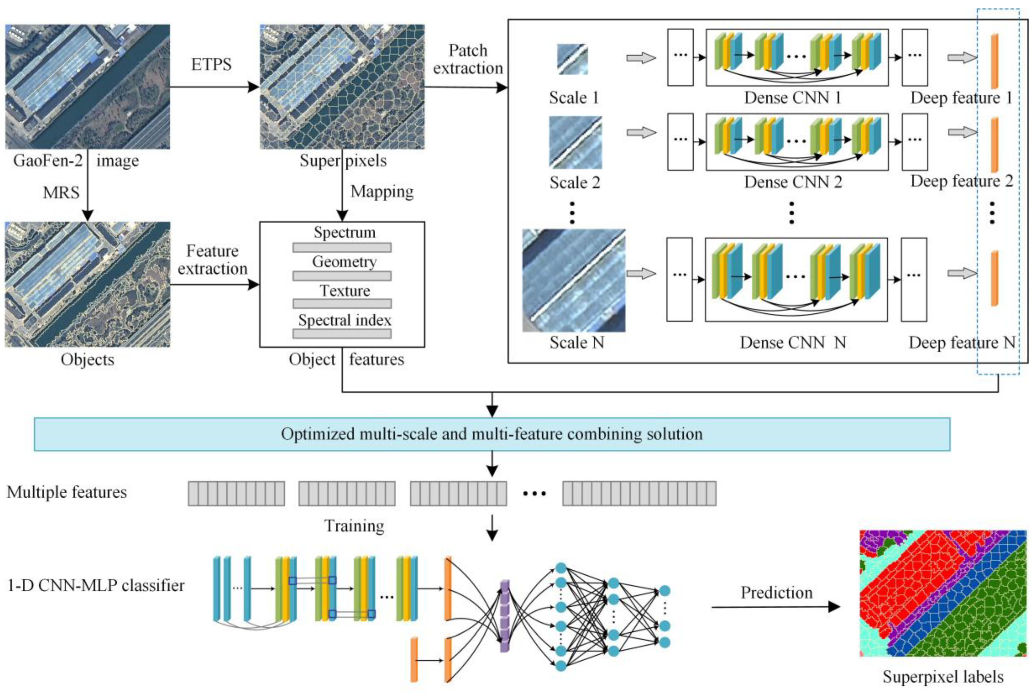
In this section, the implementation of the proposed method is illustrated concretely. The overall flowchart of our scheme is shown in Figure 2. Given an HSR multi-spectral image, superpixels were initially generated using the ETPS algorithm with false-color composition and image enhancement. Then, the multi-size patches of superpixels were selected and learned through parallel dense CNNs, and multi-scale features were extracted from GAP layers. Next, superpixel multi-scale CNN features were mapped and combined with multi-resolution segmentation (MRS) [53] object hand-delineated features. Finally, multiple features were fused for comprehensive land-cover classification upon a 1-D CNN-MLP hybrid network with channel-wise stacking and attention-based weighting design. In particular, the effect of various multi-scale and multi-feature combinations was explored to determine the optimal fusing solution.

3.1. ETPS Superpixel Segmentation

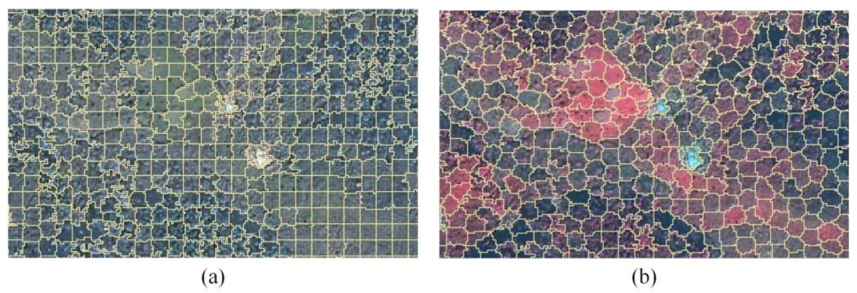
Instead of concentrating on individual pixels or irregular objects, superpixels were employed as basic units for HSR image land-cover classification in our proposed method. ETPS was designed for natural images with red, green and blue bands, whereas HSR images were multi-spectral with more than 3 bands. Standard false-color composition of images could reflect invisible environmental information and highlight the vegetation, and image enhancement using standard deviation stretching could adjust the brightness and contrast to emphasize the important content. Therefore, standard false-color composition with standard deviation stretching was employed upon original HSR images for ETPS segmentation in this study to enhance the discriminative features and boundary adherence. The comparison between ETPS segmentation based on true color and standard false-color is shown in Figure 3, using GaoFen-2 fused images with 1 m resolution in the study area. It could be observed that the boundaries of trees were easily confused with soil, crops, or grass in true color, whereas the boundaries of different vegetation categories were clearer and more accurate in standard false-color. Considering the farmland, woodland, grassland, and vacant were similar in appearance and had similar spectral characteristics, the false-color composition with information enhancement was more applicable to the ETPS method and highlighted its superiority. In addition, this approach could also better separate buildings from vegetation and produce better-fitting ground object boundaries.

3.2. Multi-Scale CNN Feature Extraction

Based on ETPS segmentation results, multi-scale patches of superpixels were extracted from original HSR images for feature learning. According to the center points of superpixels, multi-scale contextual windows were designed, including 24×24, 32×32, 40×40, 48×48, 56×56, 64×64, 72×72, 80×80, 88×88, 96×96, 104×104, and 112×112, to comprehensively explore the spatial effects and determine the optimal solution. Considering that multi-scale patches represent multi-scope spatial relationships and multi-level spatial semantics, parallel dense CNNs were designed to learn multi-scale features specifically. In the designed network structure, dense CNNs were built upon 4 dense blocks and 3 transition layers alternatively, and the number of convolutional blocks within each dense block was evaluated and set according to the complexity of land cover in images. After training parallel dense CNNs, multi-scale features were extracted from GAP layers for feature fusion and comprehensive classification. Taking an example of 80×80 patch input, the two concrete dense CNN architectures employed in this study are shown in Table 1, designed with dense blocks containing 5 (DCNN-5) and 6 (DCNN-6) convolutional blocks, respectively. In the network, the growth rate was set to 12, the initial number of feature maps was set to 24, and the compression factor was set to 0.5.

3.3. Multi-Scale and Multi-Feature Combination

Ground objects were greatly heterogeneous in shape, texture, distribution, and context. For superpixels within class boundaries, the context was relatively uniform, and larger windows were needed to make a better decision. For superpixels across class boundaries, the context became complicated and disordered, and smaller windows were required to exclude confusing noise. Hence, multi-scale feature fusion would contribute to utilizing complementary information of multiple contexts and achieve better performance. Multi-scale description of objects or superpixels was like observing them from near to far or far to near, which was more in line with the visual recognition and multi-scale nature of remote sensing. In different spatial resolutions, the ground objects showed different characteristics and patterns, and object information from the single-scale observation field was insufficient for accurate classification. It was proposed to capture multi-scale contextual information of objects to exploit their attributes and spatial distributions [21]. Multi-scale feature learning has been shown to improve the performance in scene parsing, object categorization, and so on [33]. To do a multi-scale combination, we needed to solve the two problems of what scale to combine and how to combine scales. However, it was not the best choice to combine as many as possible single-scale features together for classification because it would cause information redundancy and accuracy reduction. Considering various multi-scale combinations have different effects of spatial complementarity, it was necessary to design and find the optimal solution. Therefore, among 12 sets of single-scale features, 36 solutions of combining 4, 6, 8, 10, 12 sets of features were put forward to test and discuss the fusion effect further, as shown in Table 2. The 1st to 36th combinations corresponded to the 1st to 36th columns in the table and were expressed as COMB1 to COMB36 in the remainder of this paper.
HSR images were segmented into objects using the MRS algorithm, and spectral (i.e., mean and standard deviation of bands), geometrical (i.e., shape index, compactness, length/width, and density), textural (i.e., GLCM homogeneity, contrast, entropy, dissimilarity, correlation, angular second moment, mean, and standard deviation), and spectral index (i.e., normalized difference vegetation index (NDVI) and normalized difference water index (NDWI)) attributes were extracted from objects. To integrate features from different segmentation levels, superpixels and objects were intersected and calculated to determine the object to which each superpixel maps. The segmentation boundaries of ETPS superpixels and MRS objects both were adherent to ground objects, so the boundaries were relatively coincident, and the mapping results were corresponding. Then, the ETPS superpixels were assigned with the hand-delineated features of their mapping objects to integrate and utilize the comprehensive multi-segmentation and multi-type features. NDVI and NDWI were often used to interpret vegetation and water information from the images, respectively. NDVI and NDWI are defined as
NDVI = ( NIR R ) / ( NIR + R )
NDWI = ( G NIR ) / ( G + NIR )
where R, G, and NIR denote the red, green, and near-infrared bands of multi-spectral images, respectively.

3.4. 1-D CNN-MLP Comprehensive Classification

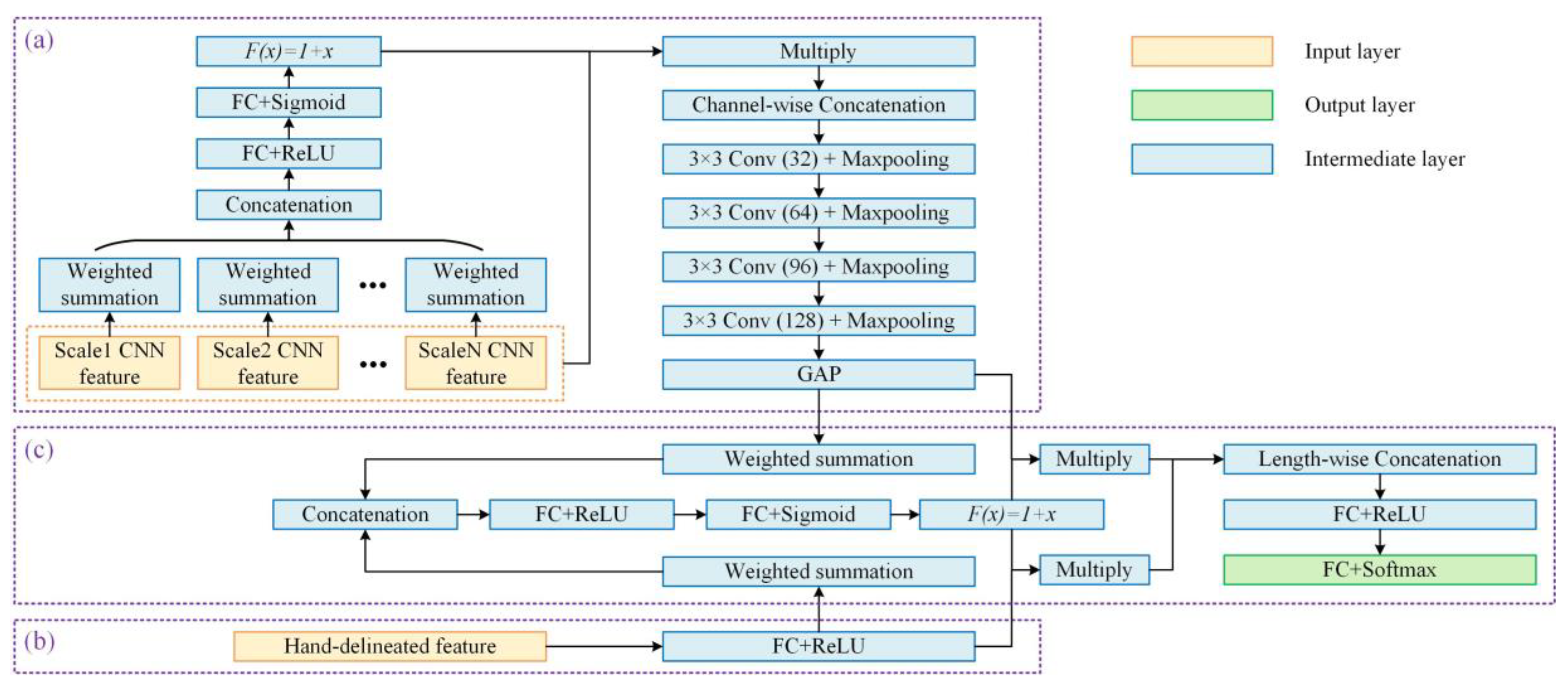
The softmax classifier used in dense CNNs was mainly for feature learning, and the 1-D CNN-MLP classifier with attention-based weighting was subsequently designed for feature fusion and final classification. Feature fusion would result in high-dimension features and intricate patterns, and there was great nonlinearity between land-cover types and multi-scale and multi-type features. The softmax classifier was simple and easy to use, but it was insufficient to fit complex relationships and not suitable for multi-scale and multi-feature fusion classification. Although SVM was good at processing large features and performed well with limited samples, it needed much more effort to optimize parameters and more time for training large datasets. Therefore, MLP, with an easy-to-adjust network structure, steady learning performance, and robust anti-noise capacity, was chosen as a comprehensive classifier. As shown in Figure 4, the hybrid network mainly consisted of 1-D CNN for multi-scale fusion and MLP for multi-feature fusion. Considering multi-scale features are interrelated vectors in the same length and feature space with various spatial semantics, channel-wise stacking and 1-D CNN were designed for feature fusion and encoding, respectively. 1-D CNN extracted cross-channel information from multi-scale sequence input through alternative 1-D convolution and max-pooling operators, and the convolutional layers with 32, 64, 96, 128 3×1 filters were employed in this study. After that, the GAP was used to further abstract the features and transform the dimension for the following multi-feature fusion. In addition, the significance of multiple scales was unbalanced for diverse superpixels, and, thus the attention-based weighting block was designed to adaptively adjust the different rate of contributions among multiple scales, instead of using equal weights. The attention block contained weighted summation for input aggregation, FC layer with ReLU for nonlinear significance evaluation, FC layer with Sigmoid for value normalization, and residual addition for value enhancement to avoid response vanishing. The attention block is calculated as
y = Concatenate ( w w s x )
z = ReLU ( w f c r y + b f c r )
s = Sigmoid ( w f c s z + b f c s )
t = s + 1
where x and w w s represent the CNN features and summation weights, respectively, y is the concatenation of multi-scale response values, w f c r , b f c r , and z denote the weights, bias, and output of the first FC layer, respectively, w f c s , b f c s , and s denote the weights, bias, and output of the second FC layer, respectively, and t is the final weighing factors for multi-scale CNN features.
In comparison, multi-scale CNN and hand-delineated features were not in the same shape and feature space, and hence they were encoded through 1-D CNN and FC layer, respectively, before multi-feature fusion. In a similar way, the encoded multi-scale and hand-delineated features were adaptively weighted using a learnable attention block to emphasize the differentiating significance for each superpixel input. After that, two types of features were combined via length-wise concatenation, and finally, FC layers with ReLU and softmax were employed for feature abstraction and classification, respectively. As a result, multi-scale CNN and hand-delineated features were efficiently and adaptively fused upon a 1-D CNN-MLP hybrid network with channel-wise stacking and attention-based weighting for comprehensive land-cover classification.

4. Experiments

4.1. Datasets

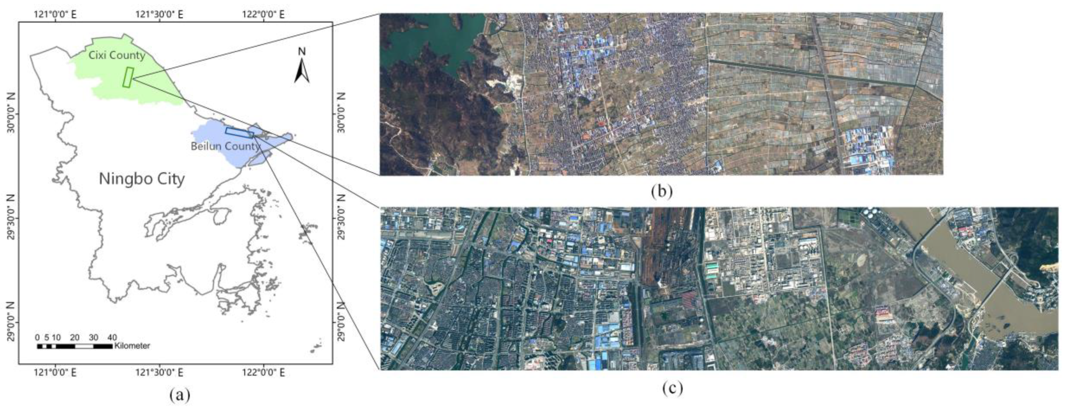
To validate the effectiveness of the proposed method, four multi-spectral HSR GaoFen-2 datasets were used for a land-cover classification demonstration. As shown in Figure 5 and Figure 6, the four datasets were located in Beilun and Cixi County of Ningbo City, Xiaoshan County of Hangzhou City, and Yuecheng County of Shaoxing City, respectively, Zhejiang Province, China. The extracted Beilun and Cixi images mainly showed the coastal urban and rural scenes, respectively, and the Xiaoshan and Yuecheng images presented the urban-rural mixed scenes. These four datasets were chosen as typical land-cover distribution scenarios to verify the applicability and generalization of our method. The Beilun and Cixi images were taken on 10 and 15 February 2016, respectively, and the Xiaoshan and Yuecheng images were taken on 12 July and 21 December 2017, respectively. All images were of 1 m resolution with 4 bands (i.e., blue, green, red, and near-infrared) and generated by the fusion of panchromatic and multi-spectral GaoFen-2 images. The land-cover ground truth was provided by the Zhejiang Provincial Bureau of Surveying and Mapping, and the data update time was 2016 for Beilun and Cixi and 2017 for Xiaoshan and Yuecheng. Manual checking was carried out to adapt the ground truth to image data.
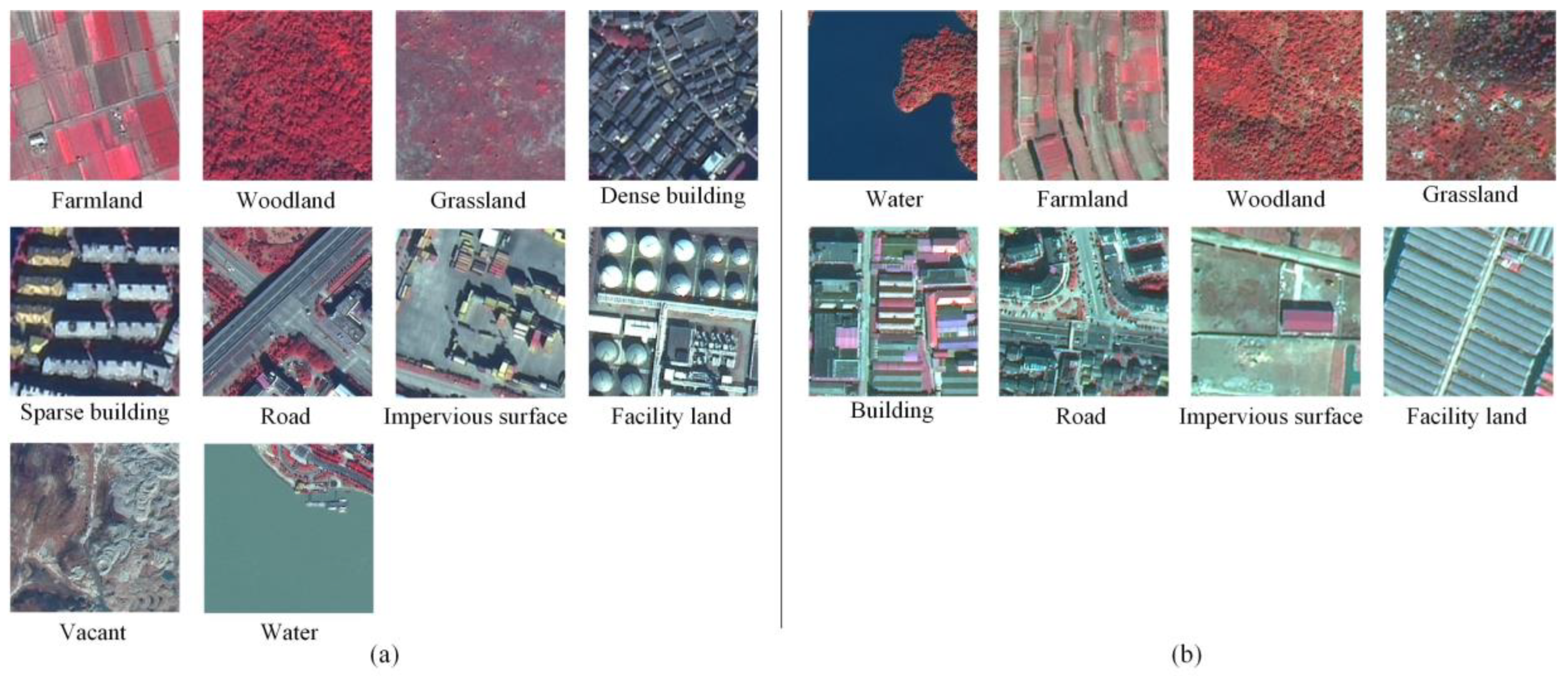
For the Beilun dataset, as shown in Figure 5c, the image covered the size of 12782×3077 m2. There were mainly 10 land-cover classes in this urban scene, including farmland, woodland, grassland, dense building, sparse building, road, impervious surface, facility land, vacant, and water. For the Cixi dataset, as shown in Figure 5b, the image covered the size of 10367×2991 m2. There were mainly 8 land-cover classes in this rural scene, including water, farmland, woodland, grassland, building, road, impervious surface, and facility land. For the Xiaoshan dataset, as shown in Figure 6b,c, the training and testing image covered the size of 7880×3855 m2, and the validating image covered the size of 5757×3086 m2. For the Yuecheng dataset, as shown in Figure 6d,e, the training and testing image covered the size of 6269×4683 m2, and the validating image covered the size of 4150×3663 m2. There were mainly 7 land-cover types in these two mixed scenes, including farmland, woodland, building, road, impervious surface, vacant, and water. Ground object examples of all classes for the Beilun and Cixi datasets are shown, for instance, in Figure 7, and sample conditions and subclass descriptions for all datasets are presented in Table 3, Table 4, Table 5, Table 6 and Table 7, respectively. The 60% and 40% of samples in Figure 5b,c, as well as Figure 6b,d, were employed for training and testing, respectively, and all samples in Figure 6c,e were adopted for validation. All samples for each dataset were normalized using the z-score approach band by band.

4.2. Parameter Settings

Considering that the land-cover categories and distribution were more intensive in Beilun dataset than the others, DCNN-6 was employed for the Beilun dataset, and DCNN-5 was adopted for Cixi, Xiaoshan, and Yuecheng datasets. The growth rate k was set to 12, and the number of filters at the first convolutional layer was set to 2k. The bottleneck width was set to 4k, and the compression factor was set to 0.5 to reduce computation and increase efficiency. Dropout with a 0.2 rate was adopted to enhance network diversity and generalization, and an Adam optimizer with default parameters [54] was used to adjust the learning rate during training. The dense CNNs were trained for 500 epochs with a batch size of 128 to learn sufficiently. In an attention-based weighting block, the number of nodes at FC layers with ReLU and Sigmoid was set to 2m and m, respectively, for nonlinear significance evaluation (m represents the number of input features). The number of nodes at FC layers for hand-delineated feature encoding and final feature abstraction was both set to 32. In object segmentation, both images were segmented using eCognition 9.0 software and MRS algorithm with 150 scale, 0.1 shape, and 0.5 compactness parameters.

4.3. Comparison Methods

Five comparison methods were employed to verify the proposed EMMCNN method for HSR image land-cover classification: object-based CNN (OCNN), patch-based CNN (PCNN), SLIC-based multi-scale CNN (SMCNN) [33], SLIC-based multi-scale and multi-feature CNN (SMMCNN) [55], and object-based random forest (ORF). Moreover, single-scale and multi-scale experiments were carried out to analyze scale effect, and single-feature and multi-feature experiments were performed to explore feature complementarity.
The OCNN and PCNN methods employed the CNN with 12 convolutional layers, 3 pooling layers, a GAP layer, and a softmax classifier. The first and second halves of convolutional layers adopted 64 and 128 3×3 filters per layer, respectively. The OCNN method extracted MRS object patches from HSR images using envelopes and scaled them to a fixed size for CNN input. Various scaled sizes were tried, and 64×64 was chosen for better performance. The multi-layer CNN was used to train and predict land-cover types for objects. The PCNN method first divided images into 24×24 grids and extracted contextual patches for CNN input. Various patch sizes were tried, and 80×80 was chosen for higher accuracy. The multi-layer CNN was used to train and predict land-cover types for patches, and land-cover types for objects were obtained through mapping with grids and majority voting [21].
The SMCNN method first performed the pixel-based multi-scale CNNs with contextual inputs in size of 15×15, 25×25, 35×35, and 45×45, and the concatenation of CNN last pooling layers was used as input to an auto-encoder. The classification was made by a softmax classifier based on the hidden layer of auto-encoder. The CNNs contained 5 convolutional layers with 50 filters and 2 max-pooling layers. Then, the SLIC algorithm was employed to segment the image into superpixels, and the segments were merged and classified using the prediction certainty of the classified pixels [33].
The SMMCNN method first performed pixel-based multi-scale CNNs with 16×16, 32×32, and 64×64 patch inputs, and the concatenation of CNN last convolutional layers was used as input to a logistic classifier. The CNNs contained 4 convolutional layers with 32, 64, 96, and 128 filters, respectively, and 4 max-pooling layers. Then, per-pixel hand-delineated features (i.e., NDVI, saturation, (NIR+R+G)/3, spectral values, and entropy) were extracted and classified using random forest (RF) with 100 trees. Finally, CNN and RF class probabilities were multiplied to result in the combined prediction [55], and SLIC segments were also employed and merged for mapping. Taking account of a large number of pixels in HSR images, pixel samples used in the SMCNN and SMMCNN were partially selected from the images for training and testing in this study.
The ORF method first segmented the image into MRS objects with 150 scale, 0.1 shape, and 0.5 compactness parameters, and the spectral, textural, geometrical, and spectral index attributes were extracted from each object. Then, it used the random forest classifier with 200 trees to train and recognize the land-cover types. The ORF method was set as a comparison method using only object hand-delineated features for classification, in order to prove the effectiveness of our proposed integrated multi-scale and multi-feature method.

4.4. Evaluation Criteria

Overall accuracy (OA), Kappa coefficient (KC), user’s accuracy (UA), producer’s accuracy (PA), and average accuracy (AA) were employed to inclusively assess the performance of the proposed and comparison methods. In addition, the confusion matrix was adopted to analyze the land-cover category confusion of classification results. It is a matrix of rows and columns in category number, where the main diagonal elements represent the correctly classified samples of each category, and the horizontal and vertical summation denote the total numbers of each type on classification and reference maps, respectively. OA is the percentage of rightly predicted pixels in all pixels, and UA and PA are the correct percentages for each class related to the classification and reference maps, respectively. If Q i j denotes the number of pixels of class i predicted to class j, then OA, UA, and PA are expressed as
OA = i Q i i i j Q i j
UA = Q i i j Q i j
PA = Q i i j Q j i
where i ,   j = 1 , 2 , ,   K and K denote the number of categories. AA is the average of UA for all classes. KC is a statistical value measuring the consistency of predicted labels and ground truth. Let N = i j Q i j represent the number of all pixels, and KC is defined as
KC = OA Q c 1 Q c
where
Q c = k ( j Q k j · i Q i k ) N · N
where k = 1 , 2 , ,   K and K denote the number of classes. The values of OA, KC, UA, PA, and AA range between 0 and 1, and the higher value indicates higher accuracy and better performance.

4.5. Experimental Analysis

The proposed EMMCNN method was compared with ETPS-based single-scale and single-feature methods using CNN (ESSCNN), OCNN, PCNN, SMCNN, SMMCNN, and ORF using OA, KC, UA, PA, and AA indicators. Single-feature settings mean land-cover classification using only CNN features, and multi-feature settings represent the classification using the fusion of CNN and hand-delineated features. The experimental results for four datasets are displayed in Table 8, Table 9, Table 10, Table 11, Table 12 and Table 13 and Figure 8, Figure 9, Figure 10, Figure 11, Figure 12 and Figure 13.

4.5.1. Beilun Dataset

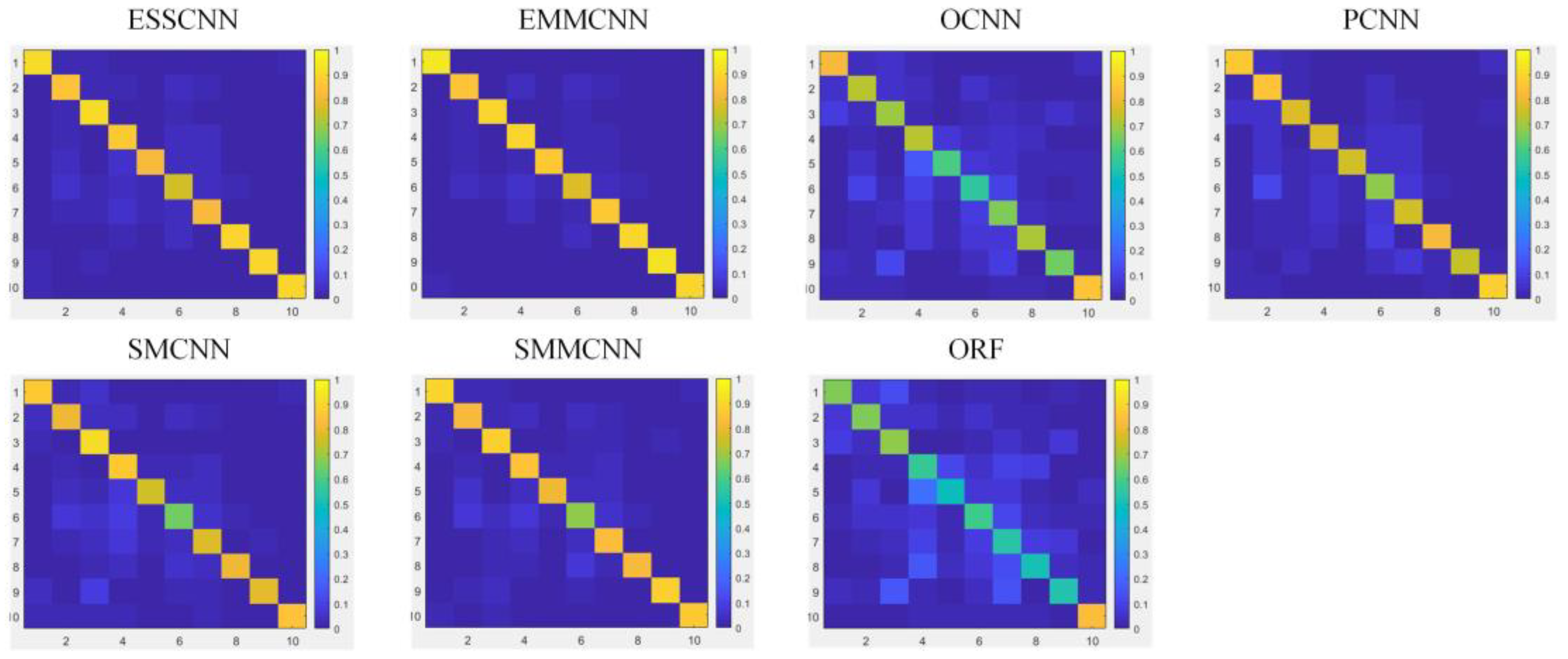
Quantitative result analysis of the Beilun dataset is shown in Table 8 and Figure 8. The EMMCNN achieved the highest OA (88.56%), KC (0.871), AA (88.59%), and UA/PA for most classes, consistently greater than the ESSCNN. The accuracy increment was much more remarkable in comparison with the OCNN, PCNN, SMCNN, SMMCNN, and ORF. Farmland, grassland, facility land, vacant, and water classes had higher accuracy, with UA/PA more than 90% for EMMCNN, whereas road class had the lowest UA/PA (77.12%/77.86%). Roads are typical linear objects distributed with other class objects along both sides, especially similar buildings and impervious surfaces, making it difficult for accurate recognition. Nonetheless, the EMMCNN method still achieved better precision in identifying roads than the compared methods. For the ESSCNN and EMMCNN methods that employed ETPS superpixels as analysis units, the classification accuracy was higher than the OCNN and PCNN methods that employed MRS objects by 7.37% to 17.99% for OA, 0.084 to 0.204 for KC, and 7.56% to 19.36% for AA, especially the woodland, sparse building, and road classes, and was higher than the SMCNN and SMMCNN methods that employed SLIC segments by 2.78% to 7.01% for OA, 0.031 to 0.079 for KC, and 3.10% to 7.24% for AA, especially the grassland and vacant classes. The performance of the EMMCNN, ESSCNN, PCNN, SMCNN, and SMMCNN methods retaining high resolution was better than the OCNN method using scaled resolution due to its information loss of spatial granularity. As a comparison method using only object attributes for classification, the ORF method had the lowest accuracy with OA 61.72%, KC 0.564, and AA 56.65%, especially the sparse building, facility land, and vacant classes. From Figure 8, it was observed that the OCNN and ORF methods tended to confuse similar artificial ground objects, such as dense buildings, sparse buildings, roads, impervious surfaces, and facility land, whereas the EMMCNN method recognized them best with the most focused values on the diagonal. The PCNN, SMCNN, and SMMCNN methods performed well on most classes except the roads, which were easily confused with impervious surface and facility land.
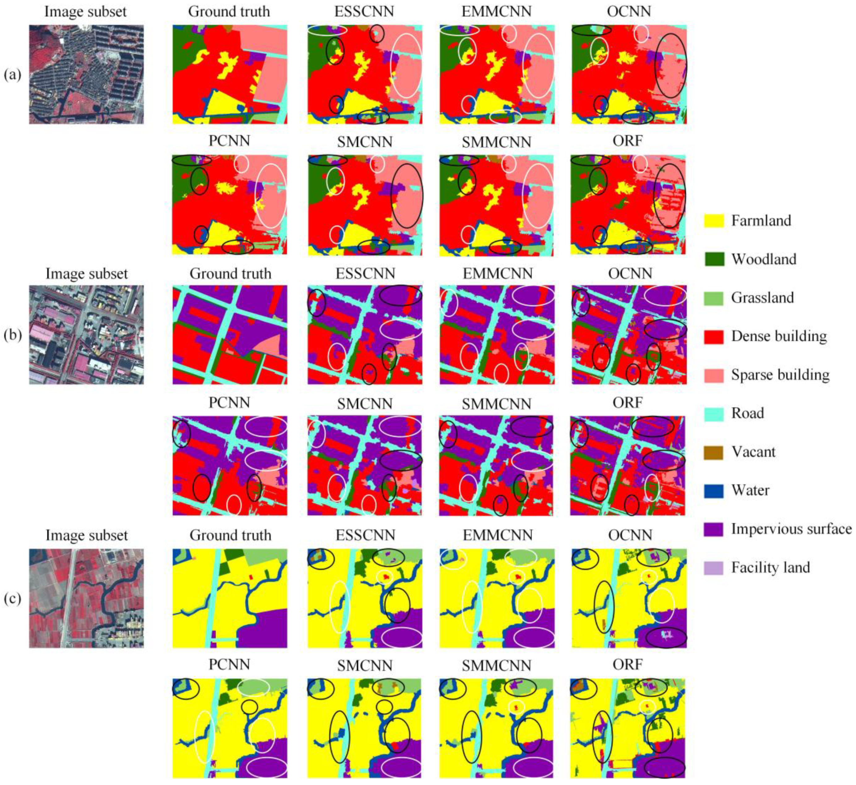
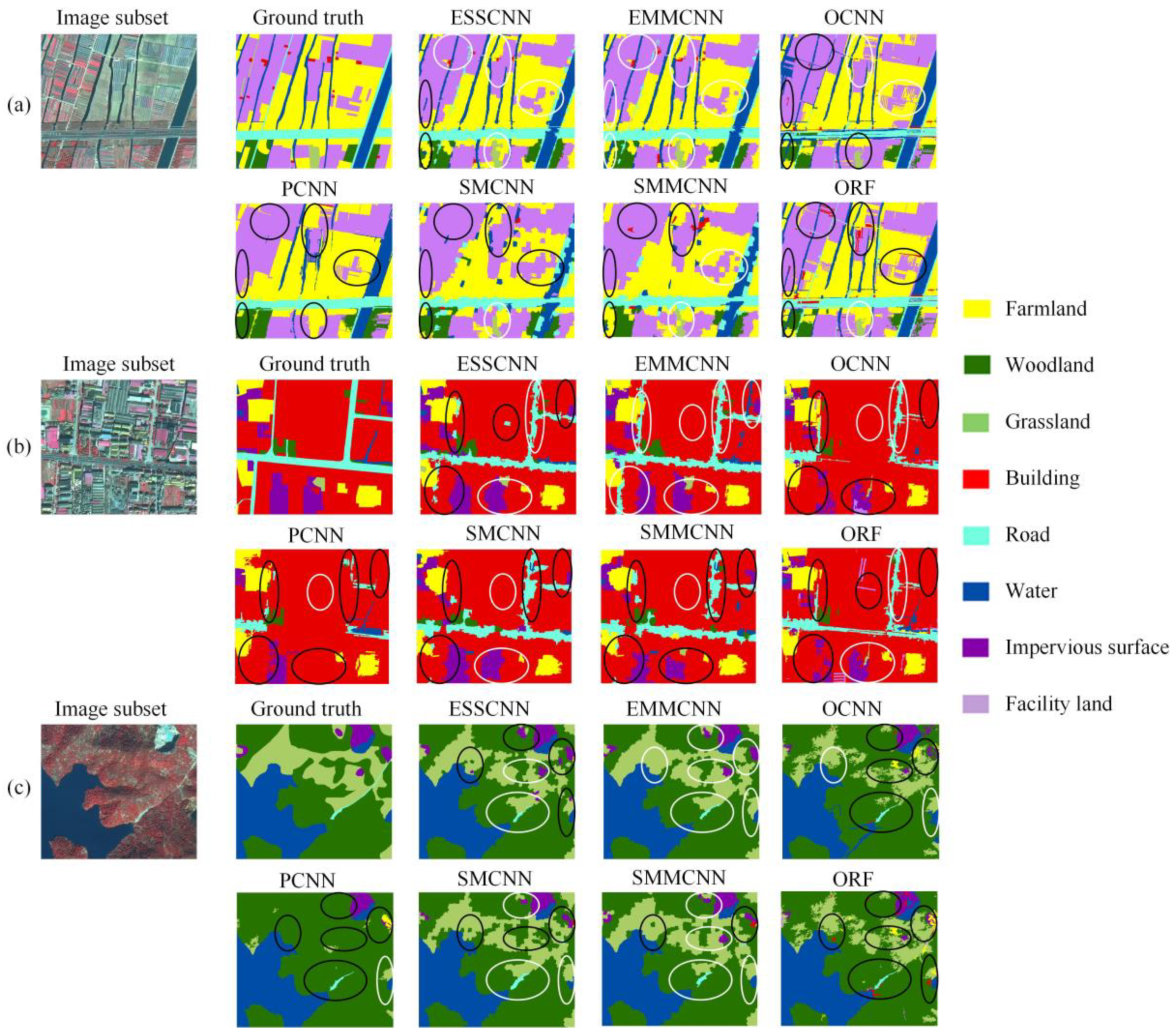
For qualitative result analysis of the Beilun dataset, as shown in Figure 9, the EMMCNN method had greater performance in not only recognizing land-cover types but also identifying class boundaries. The ESSCNN method made some mistakes in classifying small ground objects and continuous objects due to the insufficiency consideration of multi-scale contextual information and object hand-delineated features. The OCNN, PCNN, SMCNN, and SMMCNN methods had inferior performance in classifying large-scale ground objects with complex compositions and cross-class-boundary objects with variable contexts. The boundaries of the OCNN, PCNN, and ORF methods that employed MRS objects were more irregular and circuitous, and the boundaries of the SMCNN and SMMCNN methods that employed SLIC segments were less smooth and continuous. The classification result of the ORF method lacked integrity and continuity, indicating that the distribution of ground objects was not orderly enough. In summary, the experimental results of the Beilun dataset illustrated that the complementarity of multi-scale and multi-type features, the adaptability of attention-based weighting, and the learnability of dense CNNs and hybrid network promoted the EMMCNN performance for HSR image land-cover classification. The ORF, OCNN, and PCNN methods had inferior performance due to the lack of deep feature representation, the loss of original resolution information, and coarse-grained object segmentation, respectively. The SMCNN, SMMCNN, and ESSCNN methods did not achieve the best accuracy since they considered single features and limited neighborhood scales without effective parameter setting and combining solution.

4.5.2. Cixi Dataset

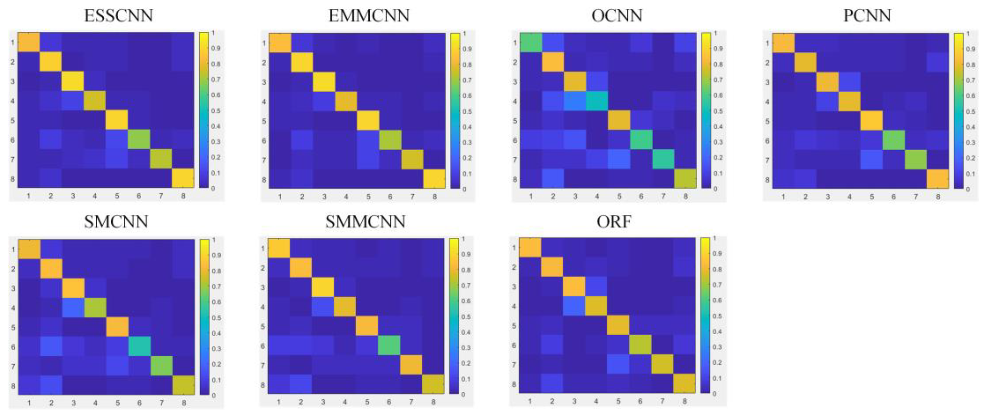
For the quantitative result analysis of the Cixi dataset, as shown in Table 9 and Figure 10, the proposed EMMCNN method obtained the best OA (88.35%), KC (0.857), AA (81.78%), and UA/PA for most classes, higher than the ESSCNN. Compared with the OCNN, PCNN, SMCNN, SMMCNN, and ORF, the improvement of EMMCNN was more dramatic. The UA/PA of farmland, woodland, and facility land classes was more than 90% for EMMCNN, whereas the UA/PA of road, impervious surface, and grassland classes was only 59.25%/70.54%, 74.00%/75.22%, and 70.39%/79.01%, respectively. In addition to linear road objects, impervious surface and grassland objects in the Cixi dataset were scattered and surrounded by analogous objects, making recognition difficult. Nonetheless, the EMMCNN method still achieved better precision of identifying them than the compared methods. For the ESSCNN and EMMCNN methods using ETPS superpixels, the classification performance was better than the OCNN and PCNN methods using MRS objects by 5.74% to 12.57% for OA, 0.074 to 0.156 for KC, and 15.48% to 22.57% for AA, especially the grassland, road and impervious surface classes, and was better than the SMCNN and SMMCNN methods using SLIC segments by 4.50% to 8.08% for OA, 0.057 to 0.101 for KC, and 10.50% to 13.76% for AA, especially the water, road, and impervious surface classes. The performance of the OCNN method with the scaled resolution was worse than the other methods with the high resolution because of the spatial information loss. As a comparison method using only object attributes for classification, the ORF method had the moderate accuracy with OA 80.77%, KC 0.761, and AA 64.15%, but the grassland, road, and impervious surface classes had much lower UA. From Figure 10, it was observed that the OCNN method tended to confuse woodland and grassland, farmland and facility land, as well as buildings and impervious surfaces. Besides the spectral similarity between these confusing classes, there were many greenhouses distributed in the farmland in the Cixi image, so the other methods also had a certain misclassification. The EMMCNN method achieved a relatively better and more balanced identification result, with more focused values on the diagonal.
For the qualitative result analysis of the Cixi dataset, as shown in Figure 11, the EMMCNN method achieved better performance in identifying land-cover types and class boundaries. The ESSCNN method had similar performance to the EMMCNN but poor in recognizing extra small objects and linear continuous objects. The SMCNN and SMMCNN methods sometimes tended to classify the constituent parts of objects as different land-cover types or omit them. The OCNN and PCNN methods had inferior performance in distinguishing objects from similar surroundings, such as identifying roads from buildings and identifying grasslands from woodlands. The ESSCNN and EMMCNN methods that used ETPS superpixels had more regular and smooth boundaries than the OCNN, PCNN, and ORF methods using MRS objects, as well as the SMCNN and SMMCNN methods using SLIC segments. In summary, the experimental results of the Cixi dataset demonstrated that the efficient superpixel segmentation, attention-based multi-scale and multi-feature fusion, and deep learning networks in EMMCNN improved the accuracy for HSR image land-cover classification. The comparison methods had inferior performance considering they used segmentation methods with coarser granularity or less boundary adherence, classified the land-cover types based on limited features and spatial scales, and lacked comprehensive parameter optimization and feature integration.

4.5.3. Xiaoshan Dataset

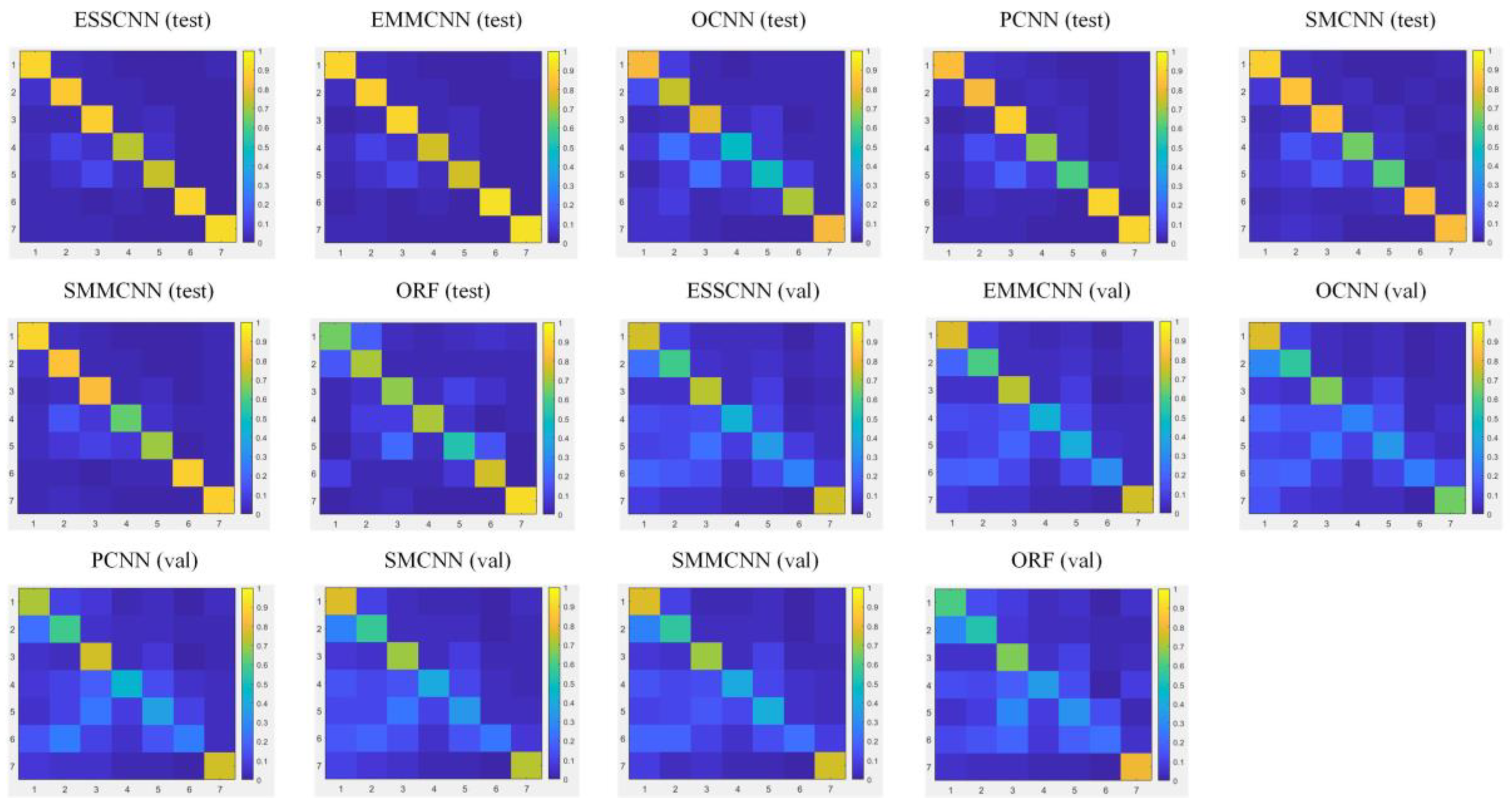
For result analysis of the Xiaoshan testing dataset, as shown in Table 10 and Figure 12, the proposed EMMCNN method achieved the best OA (88.63%), KC (0.860), AA (85.11%), and UA/PA for most classes, better than the ESSCNN. The superiority of the EMMCNN was more significant when comparing with the OCNN, PCNN, SMCNN, SMMCNN, and ORF methods. The UA/PA of farmland, vacant, and water classes was higher than 90% in EMMCNN, whereas the road and impervious surface classes had lower precision with UA/PA 69.98%/75.08% and 69.97%/76.43%, respectively. In the Xiaoshan testing dataset, the road and impervious surface objects were dispersed and mixed with other similar artificial ground objects, and the comparison methods had worse accuracy on these two classes, especially the OCNN and ORF methods. For the ESSCNN and EMMCNN methods using ETPS superpixels, the recognition accuracy was better than the OCNN and PCNN methods using MRS objects by 3.43% to 13.41% for OA, 0.043 to 0.166 for KC, and 3.92% to 16.97% for AA, and was better than the SMCNN and SMMCNN methods using SLIC segments by 2.49% to 5.47% for OA, 0.031 to 0.067 for KC, and 3.16% to 6.31% for AA. The ORF method, as a comparison method using only MRS object attributes for classification, had inferior overall performance and especially worse precision for impervious surface and vacant classes. Whereas, combining the MRS object hand-delineated features with the deep multi-scale features extracted by dense CNNs, as the auxiliary and complementary feature description, could improve the performance in the EMMCNN method. From Figure 12, it could be seen that the buildings and impervious surface, as well as woodland and roads, were relatively easier to be confused, and the ORF method had relatively worse category confusion results. The ESSCNN and EMMCNN methods had better discrimination ability with comparatively more balanced and focused values on the diagonal.
For result analysis of the Xiaoshan validating dataset, as shown in Table 11 and Figure 12, the proposed EMMCNN method achieved the highest OA (67.20%), KC (0.588), AA (57.20%), and UA/PA for most classes. The performance of the EMCNN method was better than comparison methods by 1.58% to 7.14% for OA, 0.020 to 0.095 for KC, and 1.95% to 9.17% for AA. The road, impervious surface, and vacant classes—easily confusing objects—had inferior precision, as shown in Figure 12. The farmland, building, and water classes had higher accuracy, having a relatively stable appearance and characteristics between separate areas. The accuracy of all methods for validating the dataset was worse than that for the testing dataset, considering the appearance and features of ground objects changed, and the patterns of object distribution varied in a separate area. Directly applying a trained model of one image to predict the land-cover types in another image would cause the accuracy reduction, and more efforts, such as fine-tuning, sample transferring, and feature transferring, before predicting could adjust the model and raise the performance. However, these aspects were not the focus of this article, and they would be researched in future work. In summary, the EMMCNN method achieved the best performance in both testing and validating images, owing to its hybrid network design, combining solution optimization and adaptive multi-scale and multi-feature fusion. In addition, for HSR images with complex ground objects, unbalanced land-cover types, and fragmented features, where the segment characteristics and object features changed a lot, the land-cover classification accuracy of the EMMCNN method would decrease. The parameter selection and optimization would also influence the performance of the EMMCNN method. Nonetheless, the EMMCNN method could still get relatively better accuracy with careful design and tuning in such conditions, although the improvement was reduced.

4.5.4. Yuecheng Dataset

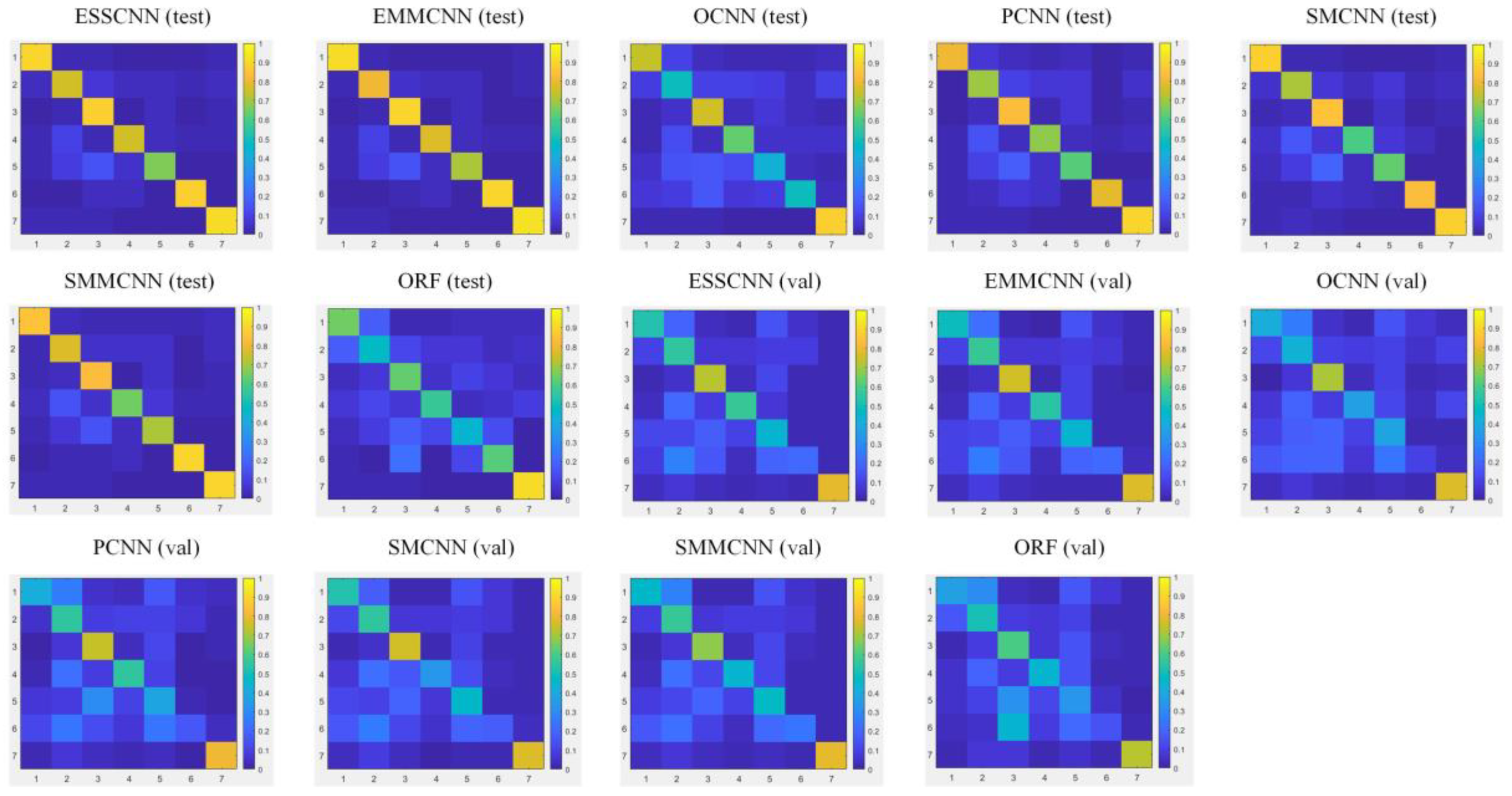
For result analysis of the Yuecheng testing dataset, as shown in Table 12 and Figure 13, the proposed EMMCNN method obtained the highest OA (87.52%), KC (0.846), AA (83.81%), and UA/PA for most classes, better than the ESSCNN. The improvement was more remarkable compared to the OCNN, PCNN, SMCNN, SMMCNN, and ORF methods. The UA/PA of farmland and water was higher than 90% in EMMCNN, and the UA/PA of impervious surface was only 64.76%/70.46%. The accuracy of road class improved in the Yuecheng dataset compared to other datasets because the road objects were wider and more complete, with more discriminative characteristics. However, the impervious surface objects in the Yuecheng dataset were more scattered and irregular, distributed among buildings, roads, and farmlands. Nonetheless, the EMMCNN method still recognized them comparatively better, and, in contrast, the OCNN and ORF methods had the worst precision. For the ESSCNN and EMMCNN methods using ETPS superpixels, the performance was better than the OCNN and PCNN methods using MRS objects by 5.32% to 16.41% for OA, 0.066 to 0.205 for KC, and 7.45% to 24.38% for AA, and was better than the SMCNN and SMMCNN methods using SLIC segments by 2.89% to 5.84% for OA, 0.037 to 0.072 for KC, and 5.50% to 8.50% for AA. The ORF method had inferior overall performance and especially lower precision for impervious surface and vacant classes. From Figure 13, it could be seen that the OCNN and ORF methods had more category confusion, whereas the ESSCNN and EMMCNN methods showed better object discrimination. The buildings, roads, and impervious surfaces were relatively easier to be confused, with similar appearance and spectral features.
For result analysis of the Yuecheng validating dataset, as shown in Table 13 and Figure 13, the proposed EMMCNN method obtained the best OA (60.93%), KC (0.521), AA (54.85%), and UA/PA for most classes. The accuracy of the EMCNN method was higher than comparison methods by 0.54% to 10.42% for OA, 0.008 to 0.127 for KC, and 0.82% to 11.24% for AA. The woodland, impervious surfaces, and vacant classes—easily confusing classes—had inferior accuracy, as displayed in Figure 13. The building and water classes, whose appearance and characteristics are relatively more stable between separate areas, had better precision. The performance of the validating dataset was worse than that of the testing dataset, which could be raised in further using transfer learning in future work. In summary, the EMMCNN method had the highest accuracy in both testing and validating images due to its flexible multi-scale and multi-type feature fusion, parameter and solution tuning, and effective network construction. In addition, the unbalance of numbers among different categories of samples would influence the model learning ability and classification result accuracy, i.e., better for majority classes and worse for minority classes. In this study, the number of samples per land-cover type was basically sufficient for network learning with at least 909 samples for training among all datasets, although the class imbalance would result in the relatively biased model prediction capabilities. The solution to a class imbalance in land-cover classification would be researched in future work, and we mainly focused on how to raise the overall performance through multi-scale and multi-feature fusion in this paper. As a result, the precision of the majority and minority categories in the EMMCNN method was generally higher than the comparison methods, showing the overall superiority of our proposed method.

5. Discussion

5.1. Evaluation of Single Spatial Scales

In the first discussion, we compared the land-cover classification accuracy using different scales of contextual information and analyze the effect of multi-feature fusion in single-scale settings. Taking Beilun and Cixi datasets, for example, as shown in Table 14, the accuracy and consistency generally improved with larger scales and more features. For vertical comparison of the Beilun dataset, the OA/KC was raised by 11.21%/0.127 and 10.99%/0.124 in single-feature and multi-feature settings, respectively, as spatial scales extended from 24 × 24 to 112 × 112. For the Cixi dataset, the OA/KC was raised by 11.11%/0.138 and 5.81%/0.072 in single-feature and multi-feature settings, respectively. The increasing accuracy became steady when the scale was larger than 80×80. This indicated that at smaller scales, the larger contextual information was important for recognizing land-cover types, whereas, at larger scales, the importance decreased because it might introduce irrelevant information. For horizontal comparison, due to the superiority of multi-feature complementation, the OA was improved by 0.15% and 1.74% on average for the Beilun and Cixi datasets, respectively, among various single scales. Additionally, the multi-feature improvement became less significant as the spatial scale increased, reflecting that a larger scale of contextual information would partially compensate for the limited perception of object features.

5.2. Evaluation of Multi-Scale Combinations

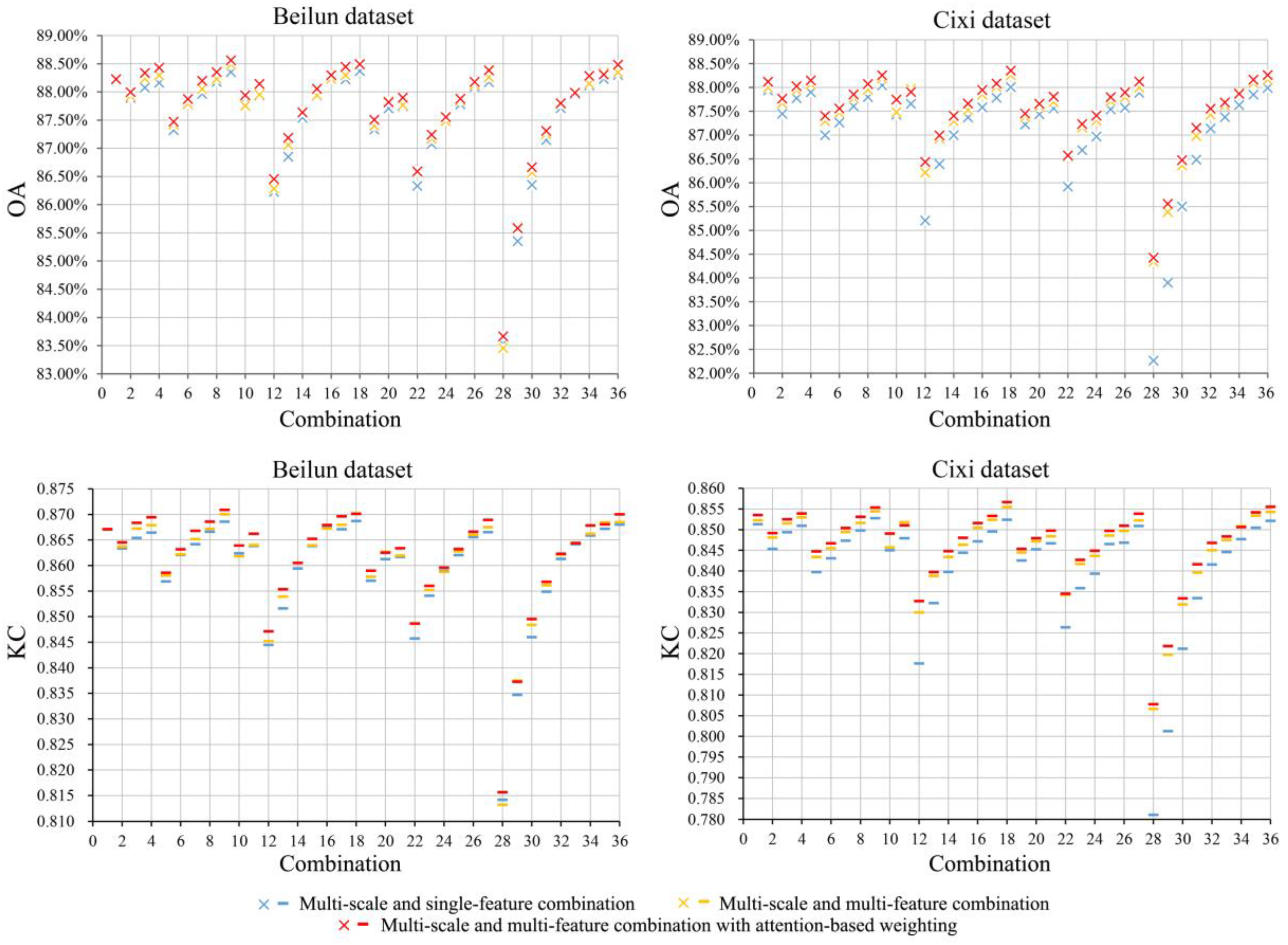
In the second discussion, we compared the performance based on different combining solutions and discussed the effect of feature fusion in multi-scale settings. Taking the Beilun and Cixi datasets, for example, a total of 36 combinations and the performance for accuracy and consistency are shown in Figure 14. For comparison among various combinations in single-feature settings, the OA/KC ranged from 83.54%/0.814 to 88.37%/0.869 and from 82.26%/0.781 to 88.04%/0.853 for the Beilun and Cixi datasets, respectively. In multi-feature settings with attention-based weighting, the OA/KC ranged from 83.67%/0.816 to 88.56%/0.871 and from 84.43%/0.808 to 88.35%/0.857 for the Beilun and Cixi datasets, respectively. For the Beilun dataset, the top five combining solutions were COMB 9, 18, 36, 17, and 4. For the Cixi dataset, the top five combinations were COMB 18, 36, 9, 35, and 4. For the Xiaoshan and Yuecheng datasets, which are not shown in the figure, the top five combinations were COMB 9, 18, 17, 4, and 35, as well as COMB 18, 9, 16, 17, and 8, respectively. It was found that most of the top combinations with better performance were composed of an appropriate number of larger scales, reflecting that it was not the best solution to combine as many scales as possible. Larger scales played a major role in promoting the combination accuracy, and smaller scales provided assisting contributions for the classification. Therefore, selecting appropriate and complementary contextual scales for the combination was important to achieve the best multi-scale performance.
For comparison among different settings, the multi-feature methods with attention-based weighting obtained the most accurate and consistent results in general. For a total of 36 combinations, the promotion of attention-based weighting classification OA/KC was 0.16%/0.002 and 0.46%/0.006 on average for the Beilun and Cixi datasets, respectively, compared to the single-feature settings, and was 0.08%/0.001 and 0.37%/0.005 on average for the Beilun and Cixi datasets, respectively, compared to the multi-feature settings without attention-based weighting. The results of multi-scale combinations were better than single-scale settings, and multi-feature fusion raised the accuracy further. In addition, the improvement of multi-feature fusion in multi-scale settings was less significant than that in single-scale settings, considering that multi-scale fusion had partially compensated for the insufficient perception of object features. In conclusion, the comprehensive classification method based on multi-scale and multi-feature fusion with attention-based weighting design had applicable importance for promoting HSR image land-cover classification.

6. Conclusions

In this paper, we presented a novel extended topology-preserving segmentation (ETPS)-based multi-scale and multi-feature method using a convolutional neural network (EMMCNN) for high spatial resolution (HSR) image land-cover classification. In the proposed scheme, HSR images were first segmented into superpixels using the ETPS algorithm with false-color composition and image enhancement to improve the boundary adherence to confusing ground objects, and parallel dense convolutional neural networks (CNNs) were built for superpixel multi-scale deep and effective feature learning. Next, superpixel multi-scale CNN features were mapped with hand-delineated features of multi-resolution segmentation (MRS) objects for complementary multi-segmentation and multi-type representation, and the effect of various multi-scale and multi-feature combinations was compared to determine the optimal solution. Finally, the multiple features were input into a hybrid network consisting of 1-dimension (1-D) CNN and multi-layer perception (MLP) with channel-wise stacking and attention-based weighting for comprehensive fusion and classification. Four real datasets of GaoFen-2 HSR images were employed for experimental demonstration. Through comparisons with ETPS-based single-scale and single-feature CNN (ESSCNN), object-based CNN (OCNN), patch-based CNN (PCNN), SLIC-based multi-scale CNN (SMCNN), SLIC-based multi-scale and multi-feature CNN (SMMCNN), and object-based random forest (ORF) methods, conclusions were drawn as follows: (1) the proposed EMMCNN achieved better performance than the compared methods considering overall accuracy (OA), Kappa coefficient (KC), average accuracy (AA) indicators, and user’s (UA) and producer’s (PA) accuracy for most classes, and it showed best results in identifying land-cover types and class boundaries; (2) for single-scale settings, the accuracy became higher as the scale extended and tended to be steady after a specific scale considering wider windows might introduce irrelevant information, and multi-feature complementation promoted the accuracy, especially at smaller scales; (3) for multi-scale settings, the performance was better when combining appropriate number of larger scales, which played a major role in promoting the integration accuracy, and multi-feature fusion raised the accuracy with attention-based weighting. This study shed light on enhancing HSR image land-cover classification using ETPS superpixels, dense CNNs, multi-scale and multi-feature fusion, and 1-D CNN-MLP hybrid network with attention-based weighting. In the future, we would focus on the exploration of class imbalance problems and the application of our scheme to transfer learning using images of different times, places, or sensors.

Author Contributions

Conceptualization, S.Z., Z.D., F.Z., and R.L.; Investigation, S.Z., C.L., S.Q., and C.G.; Methodology, S.Z.; Software, S.Z.; Validation, S.Z., Z.D., and C.L.; Formal analysis, S.Z.; Data curation, Z.D., C.L., S.Q., and C.G.; Writing—original draft preparation, S.Z.; Writing—review and editing, S.Z., Z.D., F.Z., and R.L.; Visualization, S.Z.; Supervision, Z.D.; Funding acquisition, Z.D. and R.L. All authors have read and agreed to the published version of the manuscript.

Funding

This research was funded by the National Key Research and Development Program of China, grant No. 2018YFB0505000, and supported by the Fundamental Research Funds for the Central Universities, grant No. 2019QNA3013.

Acknowledgments

The GaoFen-2 images employed in this research were provided by the Institute of Remote Sensing and Digital Earth in the Chinese Academy of Sciences, and the land-cover supporting ground data was supplied by the Zhejiang Provincial Bureau of Surveying and Mapping.

Conflicts of Interest

The authors declare no conflict of interest.

References

  1. Ma, L.; Li, M.; Ma, X.; Cheng, L.; Du, P.; Liu, Y. A review of supervised object-based land-cover image classification. ISPRS J. Photogramm. Remote Sens. 2017, 130, 277–293. [Google Scholar] [CrossRef]
  2. Zhao, W.; Du, S.; Wang, Q.; Emery, W.J. Contextually guided very-high-resolution imagery classification with semantic segments. ISPRS J. Photogramm. Remote Sens. 2017, 132, 48–60. [Google Scholar] [CrossRef]
  3. Lv, X.; Ming, D.; Chen, Y.; Wang, M. Very high resolution remote sensing image classification with SEEDS-CNN and scale effect analysis for superpixel CNN classification. Int. J. Remote Sens. 2019, 40, 506–531. [Google Scholar] [CrossRef]
  4. Kurtz, C.; Passat, N.; Gancarski, P.; Puissant, A. Extraction of complex patterns from multiresolution remote sensing images: A hierarchical top-down methodology. Pattern Recognit. 2012, 45, 685–706. [Google Scholar] [CrossRef] [Green Version]
  5. Zhao, W.; Du, S.; Emery, W.J. Object-based convolutional neural network for high-resolution imagery classification. IEEE J. Sel. Top. Appl. Earth Obs. Remote Sens. 2017, 10, 3386–3396. [Google Scholar] [CrossRef]
  6. Zhang, C.; Pan, X.; Li, H.; Gardiner, A.; Sargent, I.; Hare, J.; Atkinson, P.M. A hybrid MLP-CNN classifier for very fine resolution remotely sensed image classification. ISPRS J. Photogramm. Remote Sens. 2018, 140, 133–144. [Google Scholar] [CrossRef] [Green Version]
  7. Kelly, M.; Blanchard, S.D.; Kersten, E.; Koy, K. Terrestrial remotely sensed imagery in support of public health: New avenues of research using object-based image analysis. Remote Sens. 2011, 3, 2321–2345. [Google Scholar] [CrossRef] [Green Version]
  8. Myint, S.W.; Gober, P.; Brazel, A.; Grossman-Clarke, S.; Weng, Q. Per-pixel vs. object-based classification of urban land cover extraction using high spatial resolution imagery. Remote Sens. Environ. 2011, 115, 1145–1161. [Google Scholar] [CrossRef]
  9. Blaschke, T.; Hay, G.J.; Kelly, M.; Lang, S.; Hofmann, P.; Addink, E.; Feitosa, R.Q.; der Meer, F.; der Werff, H.; Van Coillie, F.; et al. Geographic object-based image analysis-towards a new paradigm. ISPRS J. Photogramm. Remote Sens. 2014, 87, 180–191. [Google Scholar] [CrossRef] [Green Version]
  10. Li, M.; Ma, L.; Blaschke, T.; Cheng, L.; Tiede, D. A systematic comparison of different object-based classification techniques using high spatial resolution imagery in agricultural environments. Int. J. Appl. Earth Obs. Geoinf. 2016, 49, 87–98. [Google Scholar] [CrossRef]
  11. Chen, G.; Weng, Q.; Hay, G.J.; He, Y. Geographic object-based image analysis (GEOBIA): Emerging trends and future opportunities. GIScience Remote Sens. 2018, 55, 159–182. [Google Scholar] [CrossRef]
  12. Huang, B.; Zhao, B.; Song, Y. Urban land-use mapping using a deep convolutional neural network with high spatial resolution multispectral remote sensing imagery. Remote Sens. Environ. 2018, 214, 73–86. [Google Scholar] [CrossRef]
  13. Zhang, C.; Sargent, I.; Pan, X.; Li, H.; Gardiner, A.; Hare, J.; Atkinson, P.M. An object-based convolutional neural network (OCNN) for urban land use classification. Remote Sens. Environ. 2018, 216, 57–70. [Google Scholar] [CrossRef] [Green Version]
  14. Zhang, G.; Jia, X.; Hu, J. Superpixel-based graphical model for remote sensing image mapping. IEEE Trans. Geosci. Remote Sens. 2015, 53, 5861–5871. [Google Scholar] [CrossRef]
  15. Fang, L.; Li, S.; Duan, W.; Ren, J.; Benediktsson, J.A. Classification of hyperspectral images by exploiting spectral--spatial information of superpixel via multiple kernels. IEEE Trans. Geosci. Remote Sens. 2015, 53, 6663–6674. [Google Scholar] [CrossRef] [Green Version]
  16. Fang, L.; Li, S.; Kang, X.; Benediktsson, J.A. Spectral-spatial classification of hyperspectral images with a superpixel-based discriminative sparse model. IEEE Trans. Geosci. Remote Sens. 2015, 53, 4186–4201. [Google Scholar] [CrossRef]
  17. Zhao, W.; Jiao, L.; Ma, W.; Zhao, J.; Zhao, J.; Liu, H.; Cao, X.; Yang, S. Superpixel-based multiple local CNN for panchromatic and multispectral image classification. IEEE Trans. Geosci. Remote Sens. 2017, 55, 4141–4156. [Google Scholar] [CrossRef]
  18. Feng, W.; Sui, H.; Huang, W.; Xu, C.; An, K. Water body extraction from very high-resolution remote sensing imagery using deep U-Net and a superpixel-based conditional random field model. IEEE Geosci. Remote Sens. Lett. 2018, 16, 618–622. [Google Scholar] [CrossRef]
  19. Bahmanyar, R.; Cui, S.; Datcu, M. A comparative study of bag-of-words and bag-of-topics models of EO image patches. IEEE Geosci. Remote Sens. Lett. 2015, 12, 1357–1361. [Google Scholar] [CrossRef] [Green Version]
  20. Zhao, B.; Zhong, Y.; Zhang, L. A spectral-structural bag-of-features scene classifier for very high spatial resolution remote sensing imagery. ISPRS J. Photogramm. Remote Sens. 2016, 116, 73–85. [Google Scholar] [CrossRef]
  21. Tong, X.-Y.; Xia, G.-S.; Lu, Q.; Shen, H.; Li, S.; You, S.; Zhang, L. Learning transferable deep models for land-use classification with high-resolution remote sensing images. arXiv 2018, arXiv:1807.05713. [Google Scholar]
  22. Sun, Y.; Zhang, X.; Xin, Q.; Huang, J. Developing a multi-filter convolutional neural network for semantic segmentation using high-resolution aerial imagery and LiDAR data. ISPRS J. Photogramm. Remote Sens. 2018, 143, 3–14. [Google Scholar] [CrossRef]
  23. Wang, Q.; Yuan, Z.; Du, Q.; Li, X. GETNET: A general end-to-end 2-D CNN framework for hyperspectral image change detection. IEEE Trans. Geosci. Remote Sens. 2018, 57, 3–13. [Google Scholar] [CrossRef] [Green Version]
  24. Zhang, F.; Du, B.; Zhang, L. Scene classification via a gradient boosting random convolutional network framework. IEEE Trans. Geosci. Remote Sens. 2015, 54, 1793–1802. [Google Scholar] [CrossRef]
  25. Cheng, G.; Wang, Y.; Xu, S.; Wang, H.; Xiang, S.; Pan, C. Automatic road detection and centerline extraction via cascaded end-to-end convolutional neural network. IEEE Trans. Geosci. Remote Sens. 2017, 55, 3322–3337. [Google Scholar] [CrossRef]
  26. Zhang, L.; Zhang, L.; Du, B. Deep learning for remote sensing data: A technical tutorial on the state of the art. IEEE Geosci. Remote Sens. Mag. 2016, 4, 22–40. [Google Scholar] [CrossRef]
  27. Zhu, X.X.; Tuia, D.; Mou, L.; Xia, G.-S.; Zhang, L.; Xu, F.; Fraundorfer, F. Deep learning in remote sensing: A comprehensive review and list of resources. IEEE Geosci. Remote Sens. Mag. 2017, 5, 8–36. [Google Scholar] [CrossRef] [Green Version]
  28. Ma, L.; Liu, Y.; Zhang, X.; Ye, Y.; Yin, G.; Johnson, B.A. Deep learning in remote sensing applications: A meta-analysis and review. ISPRS J. Photogramm. Remote Sens. 2019, 152, 166–177. [Google Scholar] [CrossRef]
  29. Zhou, T.; Miao, Z.; Zhang, J. Combining CNN with hand-crafted features for image classification. In Proceedings of the 2018 14th IEEE International Conference on Signal Processing (ICSP), Beijing, China, 12–16 August 2018; pp. 554–557. [Google Scholar]
  30. Cao, Q.; Zhong, Y.; Ma, A.; Zhang, L. Urban land use/land cover classification based on feature fusion fusing hyperspectral image and lidar data. In Proceedings of the IGARSS 2018-2018 IEEE International Geoscience and Remote Sensing Symposium, Valencia, Spain, 22–27 July 2018; pp. 8869–8872. [Google Scholar]
  31. Zhao, W.; Du, S. Learning multiscale and deep representations for classifying remotely sensed imagery. ISPRS J. Photogramm. Remote Sens. 2016, 113, 155–165. [Google Scholar] [CrossRef]
  32. Zhao, W.; Guo, Z.; Yue, J.; Zhang, X.; Luo, L. On combining multiscale deep learning features for the classification of hyperspectral remote sensing imagery. Int. J. Remote Sens. 2015, 36, 3368–3379. [Google Scholar] [CrossRef]
  33. Längkvist, M.; Kiselev, A.; Alirezaie, M.; Loutfi, A. Classification and segmentation of satellite orthoimagery using convolutional neural networks. Remote Sens. 2016, 8, 329. [Google Scholar] [CrossRef] [Green Version]
  34. Liang, M.; Jiao, L.; Yang, S.; Liu, F.; Hou, B.; Chen, H. Deep multiscale spectral-spatial feature fusion for hyperspectral images classification. IEEE J. Sel. Top. Appl. Earth Obs. Remote Sens. 2018, 11, 2911–2924. [Google Scholar] [CrossRef]
  35. Tian, Q.; Wan, S.; Jin, P.; Xu, J.; Zou, C.; Li, X. A novel feature fusion with self-adaptive weight method based on deep learning for image classification. In Proceedings of the Pacific Rim Conference on Multimedia, Hefei, China, 21–22 September 2018; pp. 426–436. [Google Scholar]
  36. Zhang, Y.; Huynh, C.P.; Ngan, K.N. Feature fusion with predictive weighting for spectral image classification and segmentation. IEEE Trans. Geosci. Remote Sens. 2019, 6792–6807. [Google Scholar] [CrossRef]
  37. Cheng, G.; Li, Z.; Han, J.; Yao, X.; Guo, L. Exploring hierarchical convolutional features for hyperspectral image classification. IEEE Trans. Geosci. Remote Sens. 2018, 56, 6712–6722. [Google Scholar] [CrossRef]
  38. Liu, Y.; Cao, G.; Sun, Q.; Siegel, M. Hyperspectral classification via deep networks and superpixel segmentation. Int. J. Remote Sens. 2015, 36, 3459–3482. [Google Scholar] [CrossRef]
  39. Stutz, D.; Hermans, A.; Leibe, B. Superpixels: An evaluation of the state-of-the-art. Comput. Vis. Image Underst. 2018, 166, 1–27. [Google Scholar] [CrossRef] [Green Version]
  40. Yamaguchi, K.; McAllester, D.; Urtasun, R. Efficient joint segmentation, occlusion labeling, stereo and flow estimation. In Proceedings of the European Conference on Computer Vision, Zurich, Switzerland, 6–12 September 2014; pp. 756–771. [Google Scholar]
  41. Yao, J.; Boben, M.; Fidler, S.; Urtasun, R. Real-time coarse-to-fine topologically preserving segmentation. In Proceedings of the IEEE Conference on Computer Vision and Pattern Recognition, Boston, America, 8–10 June 2015; pp. 2947–2955. [Google Scholar]
  42. LeCun, Y.; Bottou, L.; Bengio, Y.; Haffner, P. Gradient-based learning applied to document recognition. Proc. IEEE 1998, 86, 2278–2324. [Google Scholar] [CrossRef] [Green Version]
  43. Krizhevsky, A.; Sutskever, I.; Hinton, G.E. Imagenet classification with deep convolutional neural networks. In Proceedings of the Advances in Neural Information Processing Systems; Neural Information Processing Systems Foundation, Inc.: Lake Tahoe, America, 2012; pp. 1097–1105. [Google Scholar]
  44. Simonyan, K.; Zisserman, A. Very deep convolutional networks for large-scale image recognition. arXiv 2014, arXiv:1409.1556. [Google Scholar]
  45. He, K.; Zhang, X.; Ren, S.; Sun, J. Deep residual learning for image recognition. In Proceedings of the IEEE Conference on Computer Vision and Pattern Recognition, Las Vegas, America, 27–30 June 2016; pp. 770–778. [Google Scholar]
  46. Huang, G.; Liu, Z.; Van Der Maaten, L.; Weinberger, K.Q. Densely connected convolutional networks. In Proceedings of the IEEE Conference on Computer Vision and Pattern Recognition, Honolulu, America, 22–25 July 2017; pp. 4700–4708. [Google Scholar]
  47. Han, X.; Zhong, Y.; Cao, L.; Zhang, L. Pre-trained Alexnet architecture with pyramid pooling and supervision for high spatial resolution remote sensing image scene classification. Remote Sens. 2017, 9, 848. [Google Scholar] [CrossRef] [Green Version]
  48. Anwer, R.M.; Khan, F.S.; van de Weijer, J.; Molinier, M.; Laaksonen, J. Binary patterns encoded convolutional neural networks for texture recognition and remote sensing scene classification. ISPRS J. Photogramm. Remote Sens. 2018, 138, 74–85. [Google Scholar] [CrossRef] [Green Version]
  49. Xu, Y.; Xie, Z.; Feng, Y.; Chen, Z. Road extraction from high-resolution remote sensing imagery using deep learning. Remote Sens. 2018, 10, 1461. [Google Scholar] [CrossRef] [Green Version]
  50. Tao, Y.; Xu, M.; Lu, Z.; Zhong, Y. DenseNet-based depth-width double reinforced deep learning neural network for high-resolution remote sensing image per-pixel classification. Remote Sens. 2018, 10, 779. [Google Scholar] [CrossRef] [Green Version]
  51. Mahdianpari, M.; Salehi, B.; Rezaee, M.; Mohammadimanesh, F.; Zhang, Y. Very deep convolutional neural networks for complex land cover mapping using multispectral remote sensing imagery. Remote Sens. 2018, 10, 1119. [Google Scholar] [CrossRef] [Green Version]
  52. Ioffe, S.; Szegedy, C. Batch normalization: Accelerating deep network training by reducing internal covariate shift. arXiv 2015, arXiv:1502.03167. [Google Scholar]
  53. Benz, U.C.; Hofmann, P.; Willhauck, G.; Lingenfelder, I.; Heynen, M. Multi-resolution, object-oriented fuzzy analysis of remote sensing data for GIS-ready information. ISPRS J. Photogramm. Remote Sens. 2004, 58, 239–258. [Google Scholar] [CrossRef]
  54. Kingma, D.P.; Ba, J. Adam: A method for stochastic optimization. arXiv 2014, arXiv:1412.6980. [Google Scholar]
  55. Paisitkriangkrai, S.; Sherrah, J.; Janney, P.; Hengel, V.-D. Others Effective semantic pixel labelling with convolutional networks and conditional random fields. In Proceedings of the IEEE Conference on Computer Vision and Pattern Recognition Workshops, Boston, America, 11–12 June 2015; pp. 36–43. [Google Scholar]
Figure 1. DenseNet architecture with dense blocks and transition layers.
Remotesensing 12 00066 g001
Figure 2. Flowchart of the proposed extended topology-preserving segmentation (ETPS)-based multi-scale and multi-feature method using the convolutional neural network (CNN) for high spatial resolution (HSR) image land-cover classification.
Remotesensing 12 00066 g002
Figure 3. Comparison of superpixel segmentation using extended topology-preserving segmentation (ETPS)based on different color compositions. (a) ETPS segmentation based on true color. (b) ETPS segmentation based on standard false-color.
Remotesensing 12 00066 g003
Figure 4. 1-D CNN-MLP hybrid network with attention-based weighting design for comprehensive land-cover classification. (a) Multi-scale CNN feature fusion and encoding. (b) Hand-delineated feature encoding. (c) Multi-scale and multi-feature fusion and classification. CNN: convolutional neural network; MLP: multi-layer perception.
Remotesensing 12 00066 g004
Figure 5. Study areas (a) and GaoFen-2 images of Beilun urban scenes (c) and Cixi rural scenes (b) in true color.
Remotesensing 12 00066 g005
Figure 6. Study areas (a), GaoFen-2 images of Xiaoshan for training and testing (b) and validation (c), and GaoFen-2 images of Yuecheng for training and testing (d) and validation (e) in true color.
Remotesensing 12 00066 g006
Figure 7. Examples of different land-cover classes in false-color for Beilun and Cixi datasets. (a) Images of 10 land-cover classes in the Beilun dataset. (b) Images of 8 land-cover classes in the Cixi dataset.
Remotesensing 12 00066 g007
Figure 8. Confusion matrices of testing samples in the Beilun dataset for the ESSCNN, EMMCNN, OCNN, PCNN, SMCNN, SMMCNN, and ORF methods. The numbers 1 to 10 in horizontal and vertical axis denote the farmland, woodland, grassland, dense building, sparse building, road, impervious surface, facility land, vacant, and water classes, respectively. ESSCNN: extended topology-preserving segmentation (ETPS)-based single-scale and single-feature convolutional neural network (CNN); EMMCNN: ETPS-based multi-scale and multi-feature CNN; OCNN: object-based CNN; PCNN: patch-based CNN; SMCNN: simple linear iterative clustering (SLIC)-based multi-scale CNN; SMMCNN: SLIC-based multi-scale and multi-feature CNN; ORF: object-based random forest.
Remotesensing 12 00066 g008
Figure 9. Three typical image subsets (a, b, and c) in the Beilun dataset and their classification results using ESSCNN, EMMCNN, OCNN, PCNN, SMCNN, SMMCNN, and ORF methods. The white and black circles denote the correct and incorrect classification, respectively. ESSCNN: extended topology-preserving segmentation (ETPS)-based single-scale and single-feature convolutional neural network (CNN); EMMCNN: ETPS-based multi-scale and multi-feature CNN; OCNN: object-based CNN; PCNN: patch-based CNN; SMCNN: simple linear iterative clustering (SLIC)-based multi-scale CNN; SMMCNN: SLIC-based multi-scale and multi-feature CNN; ORF: object-based random forest.
Remotesensing 12 00066 g009
Figure 10. Confusion matrices of testing samples in the Cixi dataset for the ESSCNN, EMMCNN, OCNN, PCNN, SMCNN, SMMCNN, and ORF methods. The numbers 1 to 8 in horizontal and vertical axis denote the water, farmland, woodland, grassland, building, road, impervious surface, and facility land classes, respectively. ESSCNN: extended topology-preserving segmentation (ETPS)-based single-scale and single-feature convolutional neural network (CNN); EMMCNN: ETPS-based multi-scale and multi-feature CNN; OCNN: object-based CNN; PCNN: patch-based CNN; SMCNN: simple linear iterative clustering (SLIC)-based multi-scale CNN; SMMCNN: SLIC-based multi-scale and multi-feature CNN; ORF: object-based random forest.
Remotesensing 12 00066 g010
Figure 11. Three typical image subsets (a, b, and c) in the Cixi dataset and their classification results using ESSCNN, EMMCNN, OCNN, PCNN, SMCNN, SMMCNN, and ORF methods. The white and black circles denote the correct and incorrect classification, respectively. ESSCNN: extended topology-preserving segmentation (ETPS)-based single-scale and single-feature convolutional neural network (CNN); EMMCNN: ETPS-based multi-scale and multi-feature CNN; OCNN: object-based CNN; PCNN: patch-based CNN; SMCNN: simple linear iterative clustering (SLIC)-based multi-scale CNN; SMMCNN: SLIC-based multi-scale and multi-feature CNN; ORF: object-based random forest.
Remotesensing 12 00066 g011
Figure 12. Confusion matrices of testing (test) and validating (val) samples in the Xiaoshan dataset for the ESSCNN, EMMCNN, OCNN, PCNN, SMCNN, SMMCNN, and ORF methods. The numbers 1 to 7 in horizontal and vertical axis denote the farmland, woodland, building, road, impervious surface, vacant, and water classes, respectively. ESSCNN: extended topology-preserving segmentation (ETPS)-based single-scale and single-feature convolutional neural network (CNN); EMMCNN: ETPS-based multi-scale and multi-feature CNN; OCNN: object-based CNN; PCNN: patch-based CNN; SMCNN: simple linear iterative clustering (SLIC)-based multi-scale CNN; SMMCNN: SLIC-based multi-scale and multi-feature CNN; ORF: object-based random forest.
Remotesensing 12 00066 g012
Figure 13. Confusion matrices of testing (test) and validating (val) samples in the Yuecheng dataset for the ESSCNN, EMMCNN, OCNN, PCNN, SMCNN, SMMCNN, and ORF methods. The numbers 1 to 7 in horizontal and vertical axis denote the farmland, woodland, building, road, impervious surface, vacant, and water classes, respectively. ESSCNN: extended topology-preserving segmentation (ETPS)-based single-scale and single-feature convolutional neural network (CNN); EMMCNN: ETPS-based multi-scale and multi-feature CNN; OCNN: object-based CNN; PCNN: patch-based CNN; SMCNN: simple linear iterative clustering (SLIC)-based multi-scale CNN; SMMCNN: SLIC-based multi-scale and multi-feature CNN; ORF: object-based random forest.
Remotesensing 12 00066 g013
Figure 14. Classification accuracy comparison among single-feature, multi-feature, and multi-feature with attention-based weighting methods upon multi-scale combinations. The 1st to 36th columns of the horizontal axis represent the COMB1 to COMB36 combining solutions, as shown in Table 2. OA: overall accuracy; KC: Kappa coefficient.
Remotesensing 12 00066 g014
Table 1. Dense convolutional neural network (CNN) architecture for multi-scale feature extraction in high spatial resolution (HSR) land-cover classification.
LayersDCNN-5Output SizeDCNN-6Output Size
Convolution3 × 3 conv80 × 80, 243 × 3 conv80 × 80, 24
Dense block (1) [ 1 × 1   conv 3 × 3   conv ] × 5 80 × 80, 84 [ 1 × 1   conv 3 × 3   conv ] × 6 80 × 80, 96
Transition layer (1)1 × 1 conv80 × 80, 421 × 1 conv80 × 80, 48
2 × 2 avg pool, stride 240 × 40, 422 × 2 avg pool, stride 240 × 40, 48
Dense block (2) [ 1 × 1   conv 3 × 3   conv ] × 5 40 × 40, 102 [ 1 × 1   conv 3 × 3   conv ] × 6 40 × 40, 120
Transition layer (2)1 × 1 conv40 × 40, 511 × 1 conv40 × 40, 60
2 × 2 avg pool, stride 220 × 20, 512 × 2 avg pool, stride 220 × 20, 60
Dense block (3) [ 1 × 1   conv 3 × 3   conv ] × 5 20 × 20, 111 [ 1 × 1   conv 3 × 3   conv ] × 6 20 × 20, 132
Transition layer (3)1 × 1 conv20 × 20, 551 × 1 conv20 × 20, 66
2 × 2 avg pool, stride 210 × 10, 552 × 2 avg pool, stride 210 × 10, 66
Dense block (4) [ 1 × 1   conv 3 × 3   conv ] × 5 10 × 10, 115 [ 1 × 1   conv 3 × 3   conv ] × 6 10 × 10, 138
GAP layer10 × 10 GAP1 × 1, 11510 × 10 GAP1 × 1, 138
Classification layersoftmaxsoftmax
The “conv” and “avg pool” denote “convolution” and “average pooling”, respectively, in the table. Note that each “conv” block corresponds to the sequence of BN-ReLU-convolution.
Table 2. Multi-scale combining solutions based on single-scale convolutional neural network (CNN) features for high spatial resolution (HSR) land-cover classification.
Scale123456789101112131415161718192021222324252627282930313233343536
24×24** * * * * * *
32×32*** ** *** * * **
40×40******* * *** ** * ***
48×48******** ***** * * * ****
56×56********** ***** * * * * ****
64×64********* ******* * * * * ****
72×72********** ******* * * * ****
80×80********* * ***** * * * * ****
88×88**** ***** **** * * * ****
96×96**** *** * **** * * ***
104×104* ** *** ** * * **
112×112* * * * * * * *
The horizontal and vertical axes denote 36 combinations and 12 single scales, respectively. Each combining solution contains the spatial scales marked with “*”.
Table 3. Land-cover classes, sample numbers, and subclass descriptions in the Beilun dataset.
ClassProportionTrainTestSubclass
Farmland7.09%42622841Paddy fields, dry lands, nurseries, orchards
Woodland6.74%40562703Timber forest, shrub forest, planted forest
Grassland10.37%62364156Native grassland, planted grassland
Dense building14.65%88115873Dense high-rise and low-rise buildings
Sparse building4.67%28111874Sparse high-rise and low-rise buildings
Road11.88%71434761Highways, overpasses, streets
Impervious surface17.91%107697179Squares, stadiums, parking lots, storage fields, rolled surface
Facility land8.18%49233281Oil drums, container fields, docks, industrial facilities
Vacant5.15%30962063Digging lands, bare surface
Water13.37%80405360Rivers, rivulets, ponds, lakes
Table 4. Land-cover classes, sample numbers, and subclass descriptions in the Cixi dataset.
ClassProportionTrainTestSubclass
Water9.93%46273085Rivers, rivulets, ponds, lakes
Farmland27.62%128648576Paddy field, dry land, nursery, orchard
Woodland16.56%77145143Timber forest, shrub forest, planted forest
Grassland4.41%20561371Native grassland, planted grassland
Building20.39%94996333Low-rise and mid-rise buildings
Road3.54%16481099Streets, country roads
Impervious surface1.95%909607Threshing ground, rolled surface
Facility land15.59%72604840Greenhouses, agricultural facilities
Table 5. Land-cover classes, sample numbers, and subclass descriptions in the Xiaoshan dataset.
ClassProportionTrainTestSubclass
Farmland22.01%112007500Paddy field, dry land, nursery, orchard
Woodland21.88%111527441Timber forest, shrub forest, planted forest, grassland
Building25.48%130478602Low-rise and mid-rise buildings
Road5.92%30132019Streets, country roads
Impervious surface5.58%28361902Threshing ground, rolled surface, facility land
Vacant6.29%32082134Digging lands, bare surface
Water12.85%65274391Rivers, rivulets, ponds, lakes
Table 6. Land-cover classes, sample numbers, and subclass descriptions in the Yuecheng dataset.
ClassProportionTrainTestSubclass
Farmland20.10%100296537Paddy field, dry land, nursery, orchard
Woodland13.33%66194367Timber forest, shrub forest, planted forest, grassland
Building27.03%133458935Low-rise and mid-rise buildings
Road6.72%33312205Streets, country roads
Impervious surface6.34%31762046Threshing ground, rolled surface, facility land
Vacant5.12%24941722Digging lands, bare surface
Water21.37%104597157Rivers, rivulets, ponds, lakes
Table 7. Land-cover classes and sample numbers in Xiaoshan and Yuecheng validating datasets.
ClassXiaoshan DatasetYuecheng Dataset
ProportionValidateProportionValidate
Farmland27.13%1358114.44%5592
Woodland17.95%898619.89%7704
Building27.52%1377329.18%11303
Road4.81%24087.66%2966
Impervious surface7.57%378714.34%5556
Vacant2.85%14284.55%1763
Water12.17%60919.95%3855
Table 8. Classification accuracy comparison amongst ESSCNN, EMMCNN, OCNN, PCNN, SMCNN, SMMCNN, and ORF methods for the Beilun dataset.
Land-CoverESSCNNEMMCNNOCNNPCNNSMCNNSMMCNNORF
UAPAUAPAUAPAUAPAUAPAUAPAUAPA
Farmland92.05%91.51%92.68%93.81%76.93%82.16%85.23%86.86%89.09%87.49%91.57%89.70%73.04%66.67%
Woodland81.55%84.97%85.69%85.53%68.86%71.91%64.12%85.60%79.91%79.83%79.14%81.71%72.75%66.66%
Grassland86.32%90.72%90.41%90.27%73.79%69.71%85.77%77.96%73.72%91.70%82.79%88.21%64.19%67.44%
Dense building88.76%87.39%89.85%90.01%76.90%72.65%88.94%76.81%82.41%87.20%86.61%85.19%75.19%56.54%
Sparse building83.15%82.12%86.37%86.52%57.21%60.16%75.80%75.09%74.73%75.83%77.35%80.22%23.02%48.62%
Road73.61%75.61%77.12%77.86%57.99%56.16%55.22%68.00%72.31%65.60%71.78%68.61%52.76%58.03%
Impervious surface86.89%82.40%87.56%87.45%66.29%65.76%76.57%76.13%82.09%77.86%80.94%83.54%54.37%53.66%
Facility land89.73%89.93%92.51%90.49%66.99%71.61%85.34%82.24%88.67%80.37%89.86%82.53%33.85%51.16%
Vacant92.09%89.21%92.05%93.33%65.96%64.85%89.38%74.38%79.50%79.41%82.41%87.72%32.66%52.54%
Water90.10%90.40%91.69%90.57%81.39%85.57%82.37%88.81%91.02%84.56%90.82%87.46%84.72%83.47%
AA86.43%88.59%69.23%78.87%81.35%83.33%56.65%
OA86.45%88.56%70.57%79.08%81.55%83.67%61.72%
KC0.8470.8710.6670.7630.7920.8160.564
The bold font highlights the best accuracy for AA, OA, and KC among various methods. The ESSCNN and EMMCNN performance in the table correspond to the best tests among various spatial scales and different scale combinations, respectively. ESSCNN: extended topology-preserving segmentation (ETPS)-based single-scale and single-feature convolutional neural network (CNN); EMMCNN: ETPS-based multi-scale and multi-feature CNN; OCNN: object-based CNN; PCNN: patch-based CNN; SMCNN: simple linear iterative clustering (SLIC)-based multi-scale CNN; SMMCNN: SLIC-based multi-scale and multi-feature CNN; ORF: object-based random forest. UA: user’s accuracy; PA: producer’s accuracy; AA: average accuracy; OA: overall accuracy; KC: Kappa coefficient.
Table 9. Classification accuracy comparison amongst ESSCNN, EMMCNN, OCNN, PCNN, SMCNN, SMMCNN, and ORF methods for the Cixi dataset.
Land-CoverESSCNNEMMCNNOCNNPCNNSMCNNSMMCNNORF
UAPAUAPAUAPAUAPAUAPAUAPAUAPA
Water83.59%81.99%84.46%82.89%69.11%61.27%64.94%82.52%61.03%80.14%59.67%86.25%81.49%83.82%
Farmland90.19%88.02%90.29%90.02%75.94%83.21%91.29%78.63%80.28%83.41%86.62%83.87%87.26%82.35%
Woodland91.89%90.77%92.63%92.13%85.48%78.19%91.14%80.52%88.22%85.88%88.66%89.67%87.22%83.49%
Grassland59.47%75.45%70.39%79.01%20.79%48.83%19.33%78.41%47.83%71.71%49.26%79.02%19.12%77.63%
Building92.33%89.25%92.89%89.65%91.51%79.16%92.04%86.08%92.72%82.10%94.19%82.28%91.55%79.53%
Road57.68%67.39%59.25%70.54%13.64%58.41%24.31%65.00%35.74%52.48%33.16%62.42%45.98%72.21%
Impervious surface65.27%72.87%74.00%75.22%32.28%54.80%39.37%67.93%48.24%66.60%41.21%79.99%18.16%75.67%
Facility land89.39%89.92%90.32%90.20%84.93%71.92%83.59%83.51%90.11%74.34%93.04%76.43%82.40%76.98%
AA78.73%81.78%59.21%63.25%68.02%68.23%64.15%
OA87.13%88.35%75.78%81.39%80.27%82.63%80.77%
KC0.8410.8570.7010.7670.7560.7840.761
The bold font highlights the best accuracy for AA, OA, and KC among various methods. The ESSCNN and EMMCNN performance in the table correspond to the best tests among various spatial scales and different scale combinations, respectively. ESSCNN: extended topology-preserving segmentation (ETPS)-based single-scale and single-feature convolutional neural network (CNN); EMMCNN: ETPS-based multi-scale and multi-feature CNN; OCNN: object-based CNN; PCNN: patch-based CNN; SMCNN: simple linear iterative clustering (SLIC)-based multi-scale CNN; SMMCNN: SLIC-based multi-scale and multi-feature CNN; ORF: object-based random forest. UA: user’s accuracy; PA: producer’s accuracy; AA: average accuracy; OA: overall accuracy; KC: Kappa coefficient.
Table 10. Classification accuracy comparison amongst ESSCNN, EMMCNN, OCNN, PCNN, SMCNN, SMMCNN, and ORF methods for the Xiaoshan testing samples.
Land-CoverESSCNNEMMCNNOCNNPCNNSMCNNSMMCNNORF
UAPAUAPAUAPAUAPAUAPAUAPAUAPA
Farmland89.99%89.45%91.91%90.31%75.68%81.60%90.21%83.22%85.77%88.77%87.21%89.57%78.15%64.58%
Woodland86.97%86.06%88.85%88.01%70.62%74.71%83.21%82.74%81.77%84.42%83.58%85.52%65.62%71.60%
Building91.73%87.85%92.31%89.89%88.74%78.39%86.92%88.06%89.03%85.43%91.74%84.17%90.14%68.60%
Road67.82%72.71%69.98%75.08%56.46%47.71%56.36%68.36%59.34%65.16%63.96%63.60%54.99%70.69%
Impervious surface62.42%73.74%69.97%76.43%29.03%49.65%65.11%60.17%62.93%62.19%60.27%70.26%5.78%52.67%
Vacant91.06%89.20%92.10%93.01%70.20%70.41%85.12%89.44%83.32%83.31%83.42%87.58%37.78%75.28%
Water89.72%92.00%90.66%92.93%86.29%82.23%85.33%90.40%89.43%84.03%87.40%88.15%81.86%90.76%
AA82.81%85.11%68.14%78.89%78.80%79.65%59.19%
OA86.91%88.63%75.22%83.48%83.16%84.42%70.98%
KC0.8390.8600.6940.7960.7930.8080.634
The bold font highlights the best accuracy for AA, OA, and KC among various methods. The ESSCNN and EMMCNN performance in the table correspond to the best tests among various spatial scales and different scale combinations, respectively. ESSCNN: extended topology-preserving segmentation (ETPS)-based single-scale and single-feature convolutional neural network (CNN); EMMCNN: ETPS-based multi-scale and multi-feature CNN; OCNN: object-based CNN; PCNN: patch-based CNN; SMCNN: simple linear iterative clustering (SLIC)-based multi-scale CNN; SMMCNN: SLIC-based multi-scale and multi-feature CNN; ORF: object-based random forest. UA: user’s accuracy; PA: producer’s accuracy; AA: average accuracy; OA: overall accuracy; KC: Kappa coefficient.
Table 11. Classification accuracy comparison amongst ESSCNN, EMMCNN, OCNN, PCNN, SMCNN, SMMCNN, and ORF methods for the Xiaoshan validating samples.
Land-CoverESSCNNEMMCNNOCNNPCNNSMCNNSMMCNNORF
UAPAUAPAUAPAUAPAUAPAUAPAUAPA
Farmland65.38%75.09%67.04%77.68%51.37%77.40%69.60%71.87%58.24%76.97%57.86%77.02%63.14%60.72%
Woodland66.31%58.39%68.02%60.02%61.75%55.10%65.49%58.95%63.40%56.27%66.16%56.13%62.40%52.81%
Building83.23%72.05%83.64%72.87%83.06%67.03%76.50%75.48%82.74%69.16%85.90%69.38%76.93%66.49%
Road32.64%43.55%36.50%42.52%33.75%27.69%34.64%43.95%31.36%40.48%34.41%39.57%29.95%34.94%
Impervious surface19.65%35.59%24.48%41.94%12.29%32.88%30.15%36.84%22.22%34.06%19.42%42.02%2.62%31.93%
Vacant43.43%26.81%43.70%30.74%43.76%26.39%34.70%25.08%43.26%24.85%40.70%23.43%31.43%23.29%
Water76.03%76.41%76.99%76.47%75.60%64.67%75.71%75.89%76.61%71.92%75.21%76.41%69.72%80.97%
AA55.24%57.20%51.65%55.25%53.98%54.24%48.03%
OA65.62%67.20%60.46%65.43%63.24%64.20%60.06%
KC0.5680.5880.5070.5670.5410.5510.493
The bold font highlights the best accuracy for AA, OA, and KC among various methods. The ESSCNN and EMMCNN performance in the table correspond to the best tests among various spatial scales and different scale combinations, respectively. ESSCNN: extended topology-preserving segmentation (ETPS)-based single-scale and single-feature convolutional neural network (CNN); EMMCNN: ETPS-based multi-scale and multi-feature CNN; OCNN: object-based CNN; PCNN: patch-based CNN; SMCNN: simple linear iterative clustering (SLIC)-based multi-scale CNN; SMMCNN: SLIC-based multi-scale and multi-feature CNN; ORF: object-based random forest. UA: user’s accuracy; PA: producer’s accuracy; AA: average accuracy; OA: overall accuracy; KC: Kappa coefficient.
Table 12. Classification accuracy comparison amongst ESSCNN, EMMCNN, OCNN, PCNN, SMCNN, SMMCNN, and ORF methods for the Yuecheng testing samples.
Land-CoverESSCNNEMMCNNOCNNPCNNSMCNNSMMCNNORF
UAPAUAPAUAPAUAPAUAPAUAPAUAPA
Farmland91.60%90.34%92.96%91.90%84.36%73.73%92.93%80.02%86.99%88.92%91.68%85.05%79.13%64.13%
Woodland75.83%75.84%78.33%79.85%52.95%48.59%63.10%68.79%68.33%70.80%66.30%76.94%36.86%46.92%
Building89.61%87.56%90.69%89.29%83.56%75.09%85.15%83.28%87.35%85.73%91.02%83.25%88.16%62.81%
Road73.53%76.41%76.94%76.74%41.35%63.60%61.71%68.67%76.12%60.25%73.34%64.66%46.75%56.49%
Impervious surface59.33%65.74%64.76%70.46%25.09%42.96%40.65%61.32%42.82%63.17%42.84%70.82%8.17%44.71%
Vacant83.31%88.51%89.48%89.38%45.20%48.88%79.95%78.87%73.68%82.97%70.92%89.21%3.91%61.03%
Water92.96%91.83%93.54%93.18%83.47%88.93%90.51%89.99%92.38%87.88%91.07%89.88%86.78%91.45%
AA80.88%83.81%59.43%73.43%75.38%75.31%49.97%
OA85.62%87.52%71.11%80.30%81.68%82.73%67.19%
KC0.8220.8460.6410.7560.7740.7850.584
The bold font highlights the best accuracy for AA, OA, and KC among various methods. The ESSCNN and EMMCNN performance in the table correspond to the best tests among various spatial scales and different scale combinations, respectively. ESSCNN: extended topology-preserving segmentation (ETPS)-based single-scale and single-feature convolutional neural network (CNN); EMMCNN: ETPS-based multi-scale and multi-feature CNN; OCNN: object-based CNN; PCNN: patch-based CNN; SMCNN: simple linear iterative clustering (SLIC)-based multi-scale CNN; SMMCNN: SLIC-based multi-scale and multi-feature CNN; ORF: object-based random forest. UA: user’s accuracy; PA: producer’s accuracy; AA: average accuracy; OA: overall accuracy; KC: Kappa coefficient.
Table 13. Classification accuracy comparison amongst ESSCNN, EMMCNN, OCNN, PCNN, SMCNN, SMMCNN, and ORF methods for the Yuecheng validating samples.
Land-CoverESSCNNEMMCNNOCNNPCNNSMCNNSMMCNNORF
UAPAUAPAUAPAUAPAUAPAUAPAUAPA
Farmland67.56%52.05%69.16%49.80%63.37%40.72%81.61%40.81%60.64%52.52%75.94%46.60%74.37%36.91%
Woodland49.17%56.08%46.44%56.74%35.34%42.60%32.81%55.47%47.36%55.38%34.49%57.70%26.81%50.96%
Building80.55%73.13%81.30%76.35%76.55%71.34%77.94%74.80%76.72%75.41%83.90%68.63%86.11%60.85%
Road46.83%56.67%53.33%53.97%43.44%36.14%42.74%54.93%59.24%34.08%53.19%43.92%37.92%44.56%
Impervious surface33.89%44.27%34.38%45.27%21.27%38.60%17.49%38.38%32.17%46.70%26.22%47.58%3.04%33.73%
Vacant19.48%20.90%16.80%21.73%14.84%10.90%25.73%16.74%13.14%18.23%8.77%23.88%1.58%15.38%
Water80.71%78.61%82.52%76.96%50.49%76.65%77.75%79.92%78.44%77.75%80.06%78.55%79.91%71.91%
AA54.03%54.85%43.61%50.87%52.53%51.80%44.25%
OA60.39%60.93%50.51%55.69%58.14%58.48%52.51%
KC0.5130.5210.3940.4600.4900.4880.407
The bold font highlights the best accuracy for AA, OA, and KC among various methods. The ESSCNN and EMMCNN performance in the table correspond to the best tests among various spatial scales and different scale combinations, respectively. ESSCNN: extended topology-preserving segmentation (ETPS)-based single-scale and single-feature convolutional neural network (CNN); EMMCNN: ETPS-based multi-scale and multi-feature CNN; OCNN: object-based CNN; PCNN: patch-based CNN; SMCNN: simple linear iterative clustering (SLIC)-based multi-scale CNN; SMMCNN: SLIC-based multi-scale and multi-feature CNN; ORF: object-based random forest. UA: user’s accuracy; PA: producer’s accuracy; AA: average accuracy; OA: overall accuracy; KC: Kappa coefficient.
Table 14. Classification accuracy comparison between single-feature and multi-feature methods based on single scales.
Single-ScaleBeilun DatasetCixi Dataset
Single-FeatureMulti-FeatureSingle-FeatureMulti-Feature
OAKCOAKCOAKCOAKC
24 × 2475.24%0.720 75.56%0.724 76.02%0.703 81.73%0.774
32 × 3278.71%0.760 79.01%0.763 78.72%0.737 82.59%0.784
40 × 4081.41%0.790 81.50%0.791 80.80%0.763 83.98%0.802
48 × 4883.36%0.812 83.39%0.812 82.43%0.783 84.60%0.810
56 × 5684.82%0.829 84.97%0.830 83.73%0.800 85.52%0.822
64 × 6485.25%0.834 85.43%0.835 85.31%0.819 86.33%0.831
72 × 7285.68%0.838 85.82%0.840 85.83%0.825 86.69%0.836
80 × 8086.04%0.843 86.22%0.844 86.61%0.835 87.12%0.841
88 × 8886.20%0.844 86.39%0.847 86.57%0.834 87.08%0.841
96 × 9686.40%0.846 86.45%0.847 86.89%0.838 87.29%0.843
104 × 10486.45%0.847 86.52%0.848 86.97%0.840 87.38%0.845
112 × 11286.42%0.847 86.55%0.848 87.13%0.841 87.54%0.846
OA: overall accuracy; KC: Kappa coefficient.