Delineation of Agricultural Field Boundaries from Sentinel-2 Images Using a Novel Super-Resolution Contour Detector Based on Fully Convolutional Networks

Abstract

Boundaries of agricultural fields are important features necessary for defining the location, shape, and spatial extent of agricultural units. They are commonly used to summarize production statistics at the field level. In this study, we investigate the delineation of agricultural field boundaries (AFB) from Sentinel-2 satellite images acquired over the Flevoland province, the Netherlands, using a deep learning technique based on fully convolutional networks (FCNs). We designed a multiple dilation fully convolutional network (MD-FCN) for AFB detection from Sentinel-2 images at 10 m resolution. Furthermore, we developed a novel super-resolution semantic contour detection network (named SRC-Net) using a transposed convolutional layer in the FCN architecture to enhance the spatial resolution of the AFB output from 10 m to 5 m resolution. The SRC-Net also improves the AFB maps at 5 m resolution by exploiting the spatial-contextual information in the label space. The results of the proposed SRC-Net outperform alternative upsampling techniques and are only slightly inferior to the results of the MD-FCN for AFB detection from RapidEye images acquired at 5 m resolution.

1. Introduction

The boundaries of agricultural fields are important features that define agricultural units and allow one to spatially aggregate information about fields and their characteristics. This information includes location, shape, spatial extent, and field characteristics such as crop type, soil type, fertility, yield, and taxation. Agricultural information are important indicators to monitor agriculture policies and developments; thus, they need to be up-to-date, accurate, and reliable [1]. Mapping the spatiotemporal distribution and the characteristics of agricultural fields is paramount for their effective and sound management.

According to [2], agricultural areas refer to land suitable for agricultural practices, which include arable land, permanent cropland, and permanent grassland. Agricultural field boundaries (AFB) can be conceptualized as the natural disruptions that partition locations where a change of crop type occurs, or comparable crops naturally detach [3]. Traditionally, AFB were established through surveying techniques, which are laborious, costly, and time-consuming. Currently, the availability of very high resolution (VHR) satellite imageries and the advancement in deep learning-based image analysis have shown potential for the automated delineation of agricultural field boundaries [4]. Notwithstanding the benefits of VHR images for the delineation of agricultural field boundaries, these data are often expensive and subject to closed data sharing policies. For this reason, in this study we focus on Sentinel-2 images, which are freely available with an open data policy. Among other applications, Sentinel-2 images are extensively used for crop classification [5,6,7]. The images convey relatively good spectral information (13 spectral bands) and medium spatial resolution (up to 10 m) [8]. However, their potential for the detection and delineation of agricultural boundaries have not been fully explored, they are limited to crop land classification [6] and instance segmentation [9].

Spectral and spatial-contextual features form the basis for the detection of agricultural field boundaries. Standard edge detection methods such as the Canny detector have been applied extensively to extract edges from a variety of images [10]. Multiresolution image segmentation techniques [11] and contour detection techniques such as global probabilities of boundaries (gPb) [12] are more recent techniques that can be applied to extract edges. Multi-Resolution Segmentation (MRS) is a region-mergin segmentation technique, which merges pixels into uniform regions according to a homogeneity criterion. It stops when all possible merges exceed a predefined threshold for the homogeneity criterion. GPb combines multiscale spatial cues based on color, brightness, and texture with global image information to make predictions of boundary probabilities. Both approaches use spectral and spatial information in an unsupervised manner, so that they are designed to detect generic edges in an image. For this reason, those techniques cannot extract specific type of images edges (semantic contours), like AFB.

Deep learning in image analysis is a collection of machine learning techniques based on algorithms that can learn features such as edges and curves from a given input image to address classification problems. Examples of deep learning methods used in remote sensing are convolutional neural networks (CNNs) and fully convolutional networks (FCNs). CNNs can learn the spatial-contextual features from a 3D input volume and produce a one-dimensional (feature) vector which is connected to the fully connected layer [13]. The fully connected layer is used to predict the class labels using the features extracted by the convolutional layers. FCNs are pixel-wise classification techniques that extract hierarchical features automatically from the input image. In FCNs, fully connected layers are usually replaced by transposed convolutional layers. CNNs and FCNs have been recently used for land cover and land use classification (LCLU). For instance, in [14], CNNs are applied to identify slums’ degree of deprivation, considering different levels of deprivation including socio-economical aspects. FCN applications include detection of cadastral boundaries [15] and delineation of agricultural fields in smallholder farms [4]. Despite the wide applications of these methods in LCLU classification, their capabilities for boundary delineation have not been explored for medium resolution data such as Sentinel-2; they are limited to VHR images [4].

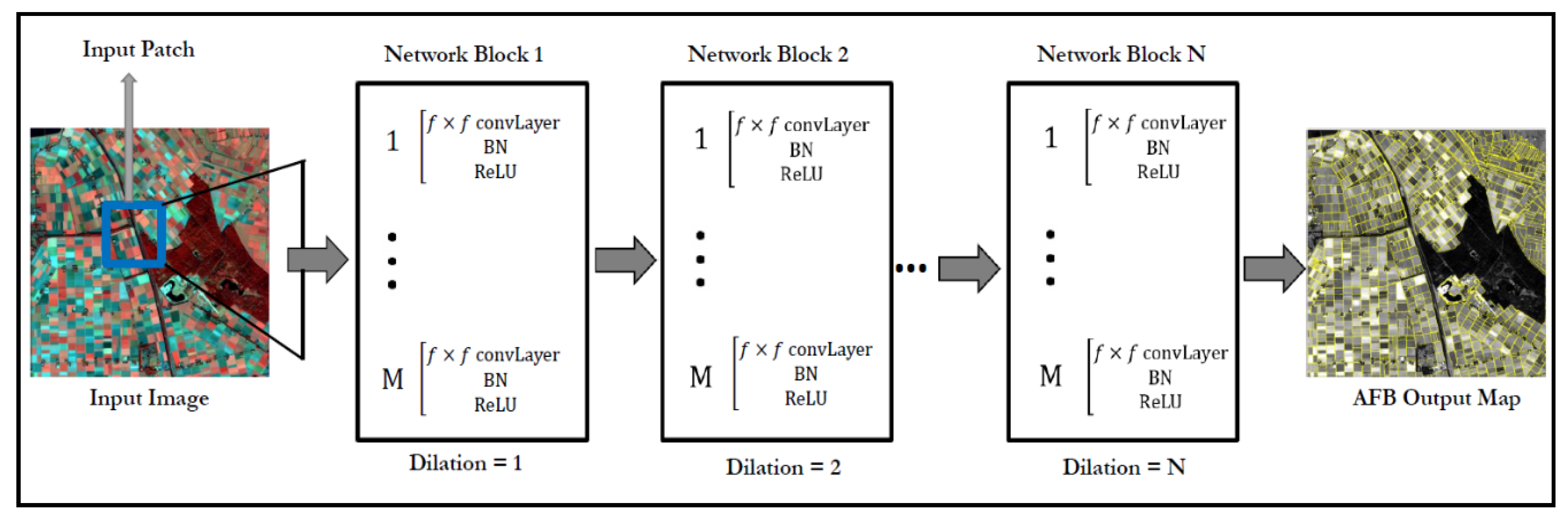
This study introduces a multiple dilation FCN (MD-FCN) for AFB delineation using free (medium resolution) Sentinel-2 images. The MD-FCN is a dilated fully convolutional network that is trained end-to-end to extract the spatial features from 10 m resolution input and produce the AFB at the same resolution. However, the spatial resolution of 10 m is relatively coarse to map the boundaries of the agricultural fields, resulting in large uncertainty in the exact location of the boundaries. 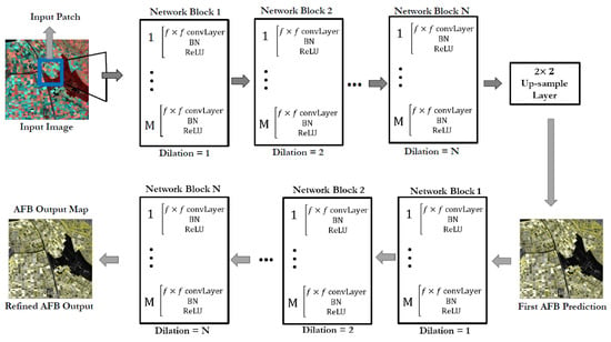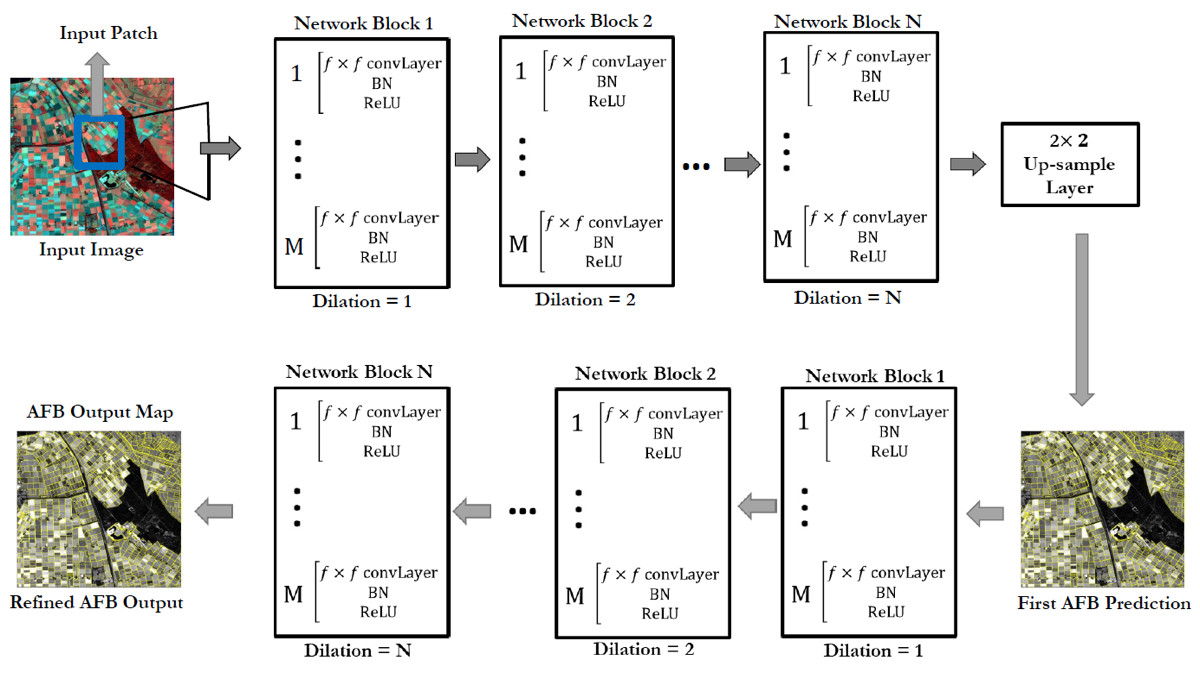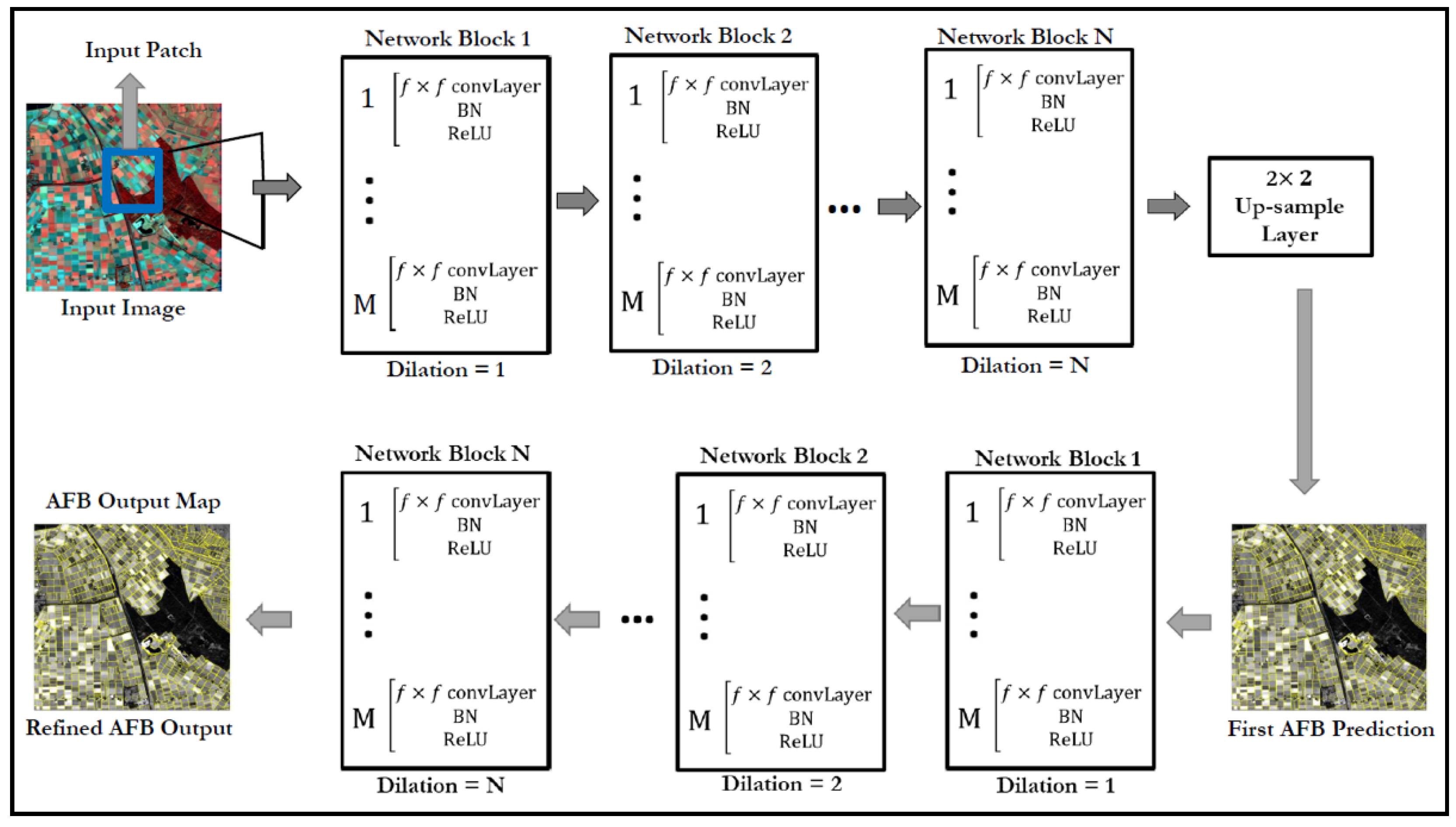Super-resolution mapping (SRM) techniques can be applied to increase the spatial resolution of the thematic map using different techniques, e.g., two-point histogram [16], Markov-random-field-based super-resolution mapping [17], and Hopfield Neural Network [18]. This paper introduces a novel super-resolution contour detector based on FCN (SRC-Net) to delineate agricultural field boundaries from Sentinel-2 images which is inspired by the idea of SRM. SRC-Net aims to learn the features from 10 m resolution images and makes predictions of the AFB at 5 m resolution. The novel method (SRC-Net) also learns the contextual features from the label space of boundaries to produce refined boundaries. We compare the performance of the SRC-Net with the results obtained from a 5 m resolution image acquired by RapidEye using MD-FCN. The aim of the comparison is to assess the performance of the SRC-Net method. In both methods (MD-FCN and SRC-Net), we address the delineation of the agricultural field boundary (AFB) as a classification problem of class AFB boundary and non-boundary.

2. Proposed Deep Fully Convolutional Networks

2.1. Multiple Dilation FCN (MD-FCN) for AFB Detection

FCNs are effective deep learning networks for pixel-wise image analysis. These networks are made up of several processing layers that are trained end-to-end to extract semantic information. The processing layers include convolution, pooling, dropout, batch normalization, and nonlinearities. As the name suggests, convolutional layers perform the main operation of the network. These layers convolve the input image with trainable filters of dimension $f\times c\times k$, where $f$ is the size of the filter kernel, $c$ is the number of the bands, and $k$ is the number of filters. Convolutional layers aim at extracting the spatial patterns present in the image which are relevant to the classification task at hand. Additionally, convolutional filters can be dilated to learn the spatial features capturing long-range pixel dependencies and maintaining a reasonably low number of parameters [19].

In this study, we designed the FCN using convolutional filters with dilated kernels. Dilated kernels are obtained by inserting zeros between filter elements, therefore expanding the spatial support of the filter without increasing the number of learnable parameters [19]. The proposed FCN is trained to extract hierarchical spatial features from the input image and transform them into the output AFB. The input to the network are image bands of the same spatial resolution; therefore, we fused the Sentinel-2 bands at 10 and 20 m resolution using bilinear interpolation and produced eight bands at 10 m spatial resolution. These bands are fed into the network as patches using a first convolutional layer. We then applied a rectified linear unit (ReLU) and batch normalization (BN) for activation and training acceleration, respectively. The output feature maps are fed as input to the next convolutional layer, then ReLU and BN follow again. The size of the feature maps is controlled by the stride factor $s$, the zero-padding parameter $p$, and the dilation factor $d$. The parameter $s$ controls the sliding of the filter to convolve the input. In this network, the stride is fixed to s = 1 because we adopted dilated convolution and no downsampling [19]. The parameter $p$ defines the number of zero-valued pixels added to the border of an input. The parameter d controls the filters by inserting zero values between the filter elements to keep the feature maps the same size as the input, hence, we set $p$ equal to $d$. The d parameter also enlarges the field of view. The series of convolutional layers, BN and ReLU operated before the last convolutional layer. The last convolutional layer is a classification layer that produces two feature maps, which are the number of classes (AFB and non-AFB class), and they are fed to the soft-max module for the prediction as an output map. This architecture is inspired and improved with respect to [19,20].

In general, the architecture of the MD-FCN for AFB detection is made up of $N$ network blocks. $N$ represents the dilation factor for each convolutional layer contained in the block. For example, the network block N = 3 applies dilation factor $d$ = 3 and the filters for all convolution layers within this block are dilated by a factor 3. Moreover, each network block can contain $M$ sub-blocks with convolution layers, BN layers, and ReLU. For both blocks (N and $M$), we prefer to use convolution layers with small $3\times 3$ filters as in the VGG network [21]. We illustrate the general architecture of the MD-FCN for AFB detection in Figure 1.

2.2. Super-Resolution Contour Detection Network (SRC-Net)

In SRC-Net, the eight-band combination of 10 m resolution from Sentinel-2 are received as input patch of the first convolutional layer. The first part of the architecture adopts the MD-FCN to extract the contour probabilities at the original resolution. The predicted probabilities are used as input to the upsampling layer which adopts a transposed convolution with a 4 × 4 filter and upsampling factor two. The upsampling is learned by the transposed convolutional layer which is trained end-to-end within the network to enhance the spatial resolution of the AFB feature maps. We used this operation to allow feature learning within the network and enable pixel-wise prediction to the feature maps at 5 m resolution. The network also regularizes the spatial contextual features and refines the exact location of the AFB by operating additional series of convolutions by using the probability of the boundary from the first prediction. The additional convolutional layers learn the contextual features from label space of the boundaries, and hence they filter the noise and increase the capability to detect more accurately the location of the contours, especially in the proximity of the corners. Figure 2 illustrates the architecture of SRC-Net.

3. Data and Experimental Analysis

3.1. Dataset Description

3.1.1. Sentinel-2 Satellite Image

We used a Sentinel-2 satellite image acquired on 26 September 2016 over Flevoland, the Netherlands. The image is in WGS 84 UTM projection, zone 31N. The original data were processed according to level 1C, which is not atmospherically corrected. We, therefore, performed an atmospheric correction to the level 2A using the Sen2Cor processor [22]. The image has 13 spectral bands, four bands at 10 m (2, 3, 4, and 8 representing Blue, Red, Green and NIR bands respectively), six bands at 20 m (5, 6, 7, and 8A representing vegetation bands; and 11 and 12 SWIR bands), and thre bands at 60 m spatial resolution (bands 1, 9, and 10 for aerosol detection, water vapor, and cirrus, respectively).

3.1.2. RapidEye Satellite Image

RapidEye data of the level 3B was acquired on 31 August 2016 covering the Flevoland. The purpose of this image was to be used as a baseline to assess and compare the accuracy obtained by the proposed SRC-Net. We downloaded RapidEye from the Planet Scope as 16 different tiles. These tiles were already orthorectified and atmospherically, radiometrically, and geometrically corrected. Then, we mosaicked the RapidEye tiles using ArcGIS software by performing “blend mosaic operation” from “Mosaic to New Raster Dataset.” In this process we used only eight relevant tiles to have an image of the area of interest (Flevoland). RapidEye data has five bands which are Blue, Red, NIR, and Red Edge (RE) and has 5 m resolution for each band with a ground sampling distance of 6.5 m.

3.1.3. Reference Data

As a reference data for AFB, we used the basic registration crop parcels (BRP) dataset from PDOK [23]. PDOK is a Dutch acronym that stands for Public Service On the Card (Publieke Dienstverlening Op de Kaart); this is a Dutch government open platform that offers up-to-date geodata. The boundaries of the agricultural parcels were constructed on the Agricultural Area Netherland (AAN). We transformed the dataset from Amersfoort/RD New projection to WGS 84 UTM zone 31N projection. The area of interest, i.e., the Flevoland province, was clipped from the entire Netherlands for further investigation. We then converted the reference data, raw BRP dataset from “Polygon To Line” using ArcGIS. We then rasterized and prepared the reference dataset using R packages raster [24], rgdal [25], and rgeos [26]. For the rasterizing, we used 10 m resolution as the finest resolution of the Sentinel-2 data.

The BRP file consists of five attributes (arable land, grassland, wasteland, natural, and other). The arable land consists of crop types and flowers. The grassland contains parcels of grasses. The wasteland contains parcels of undetermined lands and uncultivated lands due to the cultivation exemption. The natural land consists of parcels of heath which are vegetation but not agricultural field, and the other attribute contains parcels of forest which are permanent with replanting obligation and the parcels of the ditches.

We defined the agricultural field as the parcel of land used for crops and flower cultivation, together with the class grass. The grass is a recognized parcel as defined in PDOK, and it excludes ditches. In this definition of agricultural area, crops, flowers, and grass fields are considered as agricultural fields. Then, we merged the remaining three attributes and treated them as non-agricultural fields. Hence, we defined agricultural field boundary (AFB) as the outer extent that defines the transition from one agricultural field to another or from one agricultural field to a non-agricultural field. This definition of the boundary does not consider what is on the other side of the agricultural field. The boundary is the separation between the agricultural field parcels. Therefore, we categorized two classes: (1) agricultural field boundary (AFB), and (2) rest (non-boundaries).

We used reference data to create 10 tiles ground truth for training and testing the network (Figure 3). Additionally, from the Sentinel-2 image, we chose 10 tiles of the same size as the ground truth from the reference data to define the tiles for training and testing the network to detect boundaries from this data (Figure 3). We selected five tiles for training and five for testing. We cropped the tiles at 10 m resolution with a size of 800 × 800 pixels. Furthermore, we cropped 10 tiles from the RapidEye with the size of 1600 × 1600 and we cropped all tiles for ground truth and input images using R software. The tiles form the images and ground truths are overlapping in the same area.

3.2. Training the Network

We trained the networks with stochastic gradient descent algorithm using a momentum of 0.9 and a batch size of 32. We trained all network architectures in two stages, the first stage of 170 epochs with a learning rate of ${10}^{-4}$ and the second stage of 30 epochs using a learning rate ${10}^{-5}$.

3.3. Hyperparameters Sensitivity Analysis

We started the analysis by conducting preliminary experiments using only two tiles. One tile (TR1) for training and another tile (TS1) for testing the network. We performed the preliminary experiments to tune the hyperparameters including filter size, patch size, training samples, and the depth of the network (number of convolutional layers) to be used for the full dataset. We obtained the optimal hyperparameters in

Table 1. Optimal hyperparameters.

Hyperparameter	Value
Filter size	3 × 3
Patch size	55 × 55
Training sample	5000

, we then applied them for the full dataset in our analysis. For the depth of the network we obtained 20 and 34 convolutional layers as the optimal for MD-FCN and SRC-Net methods, respectively. In the SRC-Net, the 24 convolutional layers are applied for the first prediction and 10 for the later. We assessed the performance of the networks using the F-Score of the AFB output maps by comparing pixel by pixel the actual and predicted value of the AFB class label.

3.4. Accuracy Assessment

In this study, we used the F-Score accuracy measure for all experiments to evaluate the performance of the methods. F-Score is an accuracy measure that computes a harmonic average of precision (p) and recall (r) and it ranges from 0 to 1 and tends to be at best when it approaches 1 [27,28]. Precision is a measure of how close the results are to the expected result. It determines the quality of the result and recall on the other hand is a measure of completeness [28]. In this study we were interested in both the exactness and completeness measures, therefore, we used the harmonic mean, the F-Score. This accuracy assessment is a quantitative measure used by the network to evaluate the performance of the AFB output maps with their corresponding reference. For the AFB output map, this performance measure is calculated based on the four terms which are true positive, true negative, false positive, and false negative.

Precision p is the number of true positive predicted pixels of AFB divided by the number of all positive pixels returned by the network.

$$p=\frac{T_{pos}}{T_{pos}+F_{pos}}.$$

(1)

Recall r is the number of true positive predicted pixels of AFB divided by all pixels that should have been identified as positive.

$$r=\frac{T_{pos}}{T_{pos}+F_{neg}}.$$

(2)

Type I Error, and Type II Error are given by $\alpha$ and $\beta$, respectively

$$\alpha =\frac{F_{pos}}{F_{pos}+T_{neg}},$$

(3)

$$\beta =\frac{F_{neg}}{T_{pos}+F_{neg}}.$$

(4)

F-Score (F) is a harmonic average of precision ($p$) and recall ($r$). Therefore, F-Score is expressed by,

$$F=2\frac{\mathrm{pr}}{p+r}.$$

(5)

4. Results and Discussion

4.1. Multiple Dilation FCN (MD-FCN) for AFB Delineation Results

Table 2. Results of the experiments using MD-FCN for AFB delineation.

Tile	Type I Error	Type II Error	Precision	Recall	F-Score
TS1	0.04	0.36	0.66	0.64	0.65
TS2	0.05	0.44	0.64	0.56	0.60
TS3	0.05	0.40	0.66	0.60	0.63
TS4	0.05	0.34	0.69	0.66	0.67
TS5	0.05	0.42	0.67	0.58	0.62

shows the results at 10 m resolution of the AFB detection using MD-FCN. The results were obtained by the MD-FCN architecture that contains a total of 20 convolutional layers. The filter size for each convolutional layer is 3 × 3. We trained the network with 5000 patches of 55 × 55 pixels from eight input bands of 10 m resolution, 1000 from each training tile. The network produces results with an F-Score equal or higher than 0.6 for all the five test tiles. The obtained accuracy is in line with the expectations, considering the complexity of the problem of delineating the boundaries from the medium resolution data at 10 m. We notice some confusion of the parallel boundaries and some noise as shown in Figure 4.

4.2. Super-Resolution Contour Detection Network (SRC-Net) Results

Table 3. Results of the experiments using SRC-Net.

Tile	Type I Error	Type II Error	Precision	Recall	F-Score
TS1	0.03	0.61	0.43	0.39	0.41
TS2	0.04	0.63	0.46	0.37	0.41
TS3	0.04	0.64	0.45	0.36	0.40
TS4	0.04	0.59	0.46	0.41	0.43
TS5	0.04	0.64	0.47	0.36	0.41

shows the results of the SRC-Net at 5 m resolution. The results were obtained by the SRC-Net architecture that contains 24 and 10 convolutional layers for the first and second predictions, respectively. The network was trained with 500 training samples adopting 3 × 3 filters. The F-Score is equal or higher than 0.4 for all test tiles. The results are reasonable as the boundaries extracted at 10 m resolution data and produced the boundaries maps at 5 m with good location accuracy (see Figure 5).

4.3. Global Probability of Boundaries (gPb) Contour Detection

We applied gPb to obtain probabilities of boundaries by computing contour detection and performing hierarchical segmentation at scale k as applied by [12]. In this method, we investigated the threshold k by performing various experiments to get the optimal threshold for best results. We performed these preliminary experiments using the training tiles. In these experiments, the outputs are the binary maps of boundary and no-boundaries. We then analyzed these outputs visually and using the F-Score accuracy measure, and the results show that the segmentation at scale k = 0.06 performed best compared to the others. This is because, the smaller the k, the more unwanted contours detected and the larger the k the more missing contours. Therefore, we ran the technique on the full dataset by applying k = 0.06.

Table 4. Results of the experiments using global probabilities of boundaries (gPb).

Tile	Type I Error	Type II Error	Precision	Recall	F-Score
TS1	0.09	0.65	0.29	0.35	0.32
TS2	0.12	0.64	0.26	0.36	0.30
TS3	0.11	0.60	0.29	0.40	0.34
TS4	0.13	0.69	0.20	0.31	0.24
TS5	0.12	0.58	0.29	0.42	0.34

shows the F-Score accuracy and the output maps for the full dataset, respectively.

4.4. Multiresolution Image Segmentation in eCognition

We used eCognition software to detect boundaries from the eight-band combination of Sentinel-2 by applying multiresolution segmentation. The output determined by different parameters including image layers (bands) weights, composition of homogeneity criterion (shape and compactness), and scale parameter (SP). In this study, we used training tiles to investigate the SP. However, we fixed other parameters such that we gave more weight to the NIR, green and red bands for the better segmentation. This is because these bands have more details of the agricultural boundaries, therefore, we assigned weight of 3 for NIR band, 2 for green and red bands, and a weight of 1 for the remaining bands. We applied 0.5 for shape for balancing the dependence of both shape and spectral criterion, and we also applied 0.5 compactness criterion. The experiments showed that the lower the SP the smaller segments created and the higher the SP the larger the segments created. The smaller segments lead to the more unnecessary boundaries and the larger segments omit some true boundaries. Therefore, we used SP of 175 to run the full dataset and the

Table 5. Results of the experiments using multiresolution segmentation.

Tile	Type I Error	Type II Error	Precision	Recall	F-Score
TS1	0.08	0.75	0.36	0.25	0.30
TS2	0.12	0.71	0.30	0.29	0.30
TS3	0.11	0.71	0.33	0.29	0.31
TS4	0.11	0.66	0.36	0.34	0.35
TS5	0.12	0.68	0.33	0.32	0.32

presents the F-Score accuracy of the output maps.

4.5. Performance Comparison

This section presents the comparison analysis of the methods applied in this study based on the output. We analyzed these methods both visually and using the F-Score accuracy measure as accuracy assessment metric. We assessed all methods only for the class AFB boundary from the binary classes (AFB boundary and non-boundary) at 10 m and 5 m resolution.

4.5.1. Comparison of MD-FCN for AFB detection and baseline methods of global probability of boundaries (gPb) and multiresolution image segmentation (MIS) at 10 m resolution

Based on the results from the analysis, we compared the performance of MD-FCN for AFB detection with the gPb multiresolution segmentation. In general, we observed that MD-FCN performed better than the baseline methods by an increment of approximately 0.31 in the F-Score of AFB class.

Table 6. F-Score accuracy comparison of the Deep FCN and baseline method for AFB detection.

Method/Tile-F-Score	TS1	TS2	TS3	TS4	TS5	Average F-Score
MD-FCN	0.65	0.60	0.63	0.67	0.62	0.63
gPb	0.32	0.30	0.34	0.24	0.34	0.31
MIS	0.30	0.30	0.31	0.35	0.32	0.32

shows the F-Score accuracy comparison of the Deep FCN and the baseline method. Figure 6 shows their difference for all five tested tiles (TS1, TS2, TS3, TS4, and TS5). Figure 7 shows details of the the difference extracted from TS3.

4.5.2. Comparison of SRC-Net and MD-FCN for AFB detection from RapidEye at 5 m Resolution

Table 7. F-Score accuracy comparison of the Deep FCN from RapidEye and SRC-Net.

Method/Tile-F-Score	TS1	TS2	TS3	TS4	TS5	Average F-Score
MD-FCN from RapidEye	0.50	0.45	0.39	0.47	0.53	0.49
SRC-Net	0.41	0.41	0.40	0.43	0.41	0.41

presents the F-Score accuracy for the AFB output of 5 m spatial resolution using MD-FCN from RapidEye as a baseline, and SRC-Net. The MD-FCN from RapidEye performed better than SRC-Net by 7.6%. This is because MD-FCN was applied directly to the 5 m spatial resolution of the RapidEye data without upsampling, therefore the effects such as loss of fine details and visual artefacts associated with upsampling was limited.

4.5.3. Comparison of SRC-Net and nearest neighbor interpolation-based resample at 5 m Resolution

Lastly, based on the results from the analysis, we also compared the performance of SRC-Net by performing nearest neighbor-based resample on MD-FCN output at 10 m resolution. Generally, SRC-Net produced the boundaries maps with the precise location compared to the nearest neighbor-based resample that we applied to output of MD-FCN at 10 m resolution (Figure 8).

These results present a good opportunity of good spectral information from the 13 spectral bands of Sentinel-2 and potential advantages of open and free availability that overcome the using of VHR images which are commercial data. Besides, there was a negligible shift in the boundaries’ locations between input image and reference data. This shift is not fully systematic because there are some parts having shifts and others not. The shift could be the result of uncertainty in the reference dataset that does not fully agree with the satellite image. Rasterization corrected this problem but not fully and this may have contributed to the low AFB results as this study did not set any buffering between boundaries as a tolerance.

5. Discussion

Identification of the boundaries is a difficult problem, especially when the boundaries are detected from medium spatial resolution data such as Sentinel-2 images. Based on the definition of boundaries (AFB) that was adopted in this study, AFB is not necessarily associated to the object such as roads and ditches. We infer the AFB as the transition from one agricultural field to another, or from agricultural field to non-agricultural field. While roads and ditches can be possible boundaries present in the image, in this study we classified them as the non-agricultural land cover types rather than the boundaries themselves. Taking the above criteria in consideration, we therefore mapped the boundaries as the outer extent of agricultural fields, which do not have a specific size.

In this section, we discuss the results of the compared methods. We divide the discussion into three subsections. We first describe the accuracy assessment strategy followed by applicability of the methods and finally we describe the limitations of the developed methods.

5.1. Accuracy Assessment Strategies

F-Score is an accuracy assessment method commonly used to assess land cover classification maps. We used the F-score accuracy assessment test to assess the performance of our methods in detecting the agricultural field boundaries. Arguably, F-score is the desirable accuracy measure to assess the accuracy of multi-class classification through analyzing the accuracy per specific class [26], rather than assessing the overall aggregate accuracy for all classes. In this study, our aim was to assess the performance of the methods in detecting the agricultural field boundaries, and we considered the boundaries as one class against the rest. This is because there are unbalanced classes, i.e., the class boundary is much smaller than the class non-boundaries. Thus, in this specific case, the F-score was an appropriate and reliable accuracy assessment method such that it balances the size of the two classes.

In this study, we assessed the accuracy of the method outputs against reference data. The reference data was rasterized from its original format vector to allow for the automatic accuracy analysis from the FCN method. The FCN method employs the pixel by pixel comparison to assess for the accuracy of classification results from the reference data. Despite the wide application of this method and its automated performance, the pixel by pixel approach requires that both (classification output and reference) are in raster format, thus forces the rasterization of the reference data. Ordinarily, rasterization of vector data, especially polyline vector, results in the loss of data quality due to the stair-like structure of the rasterized lines. Such quality loss may damage the accuracy assessment. Using vector data as the reference data for accuracy assessment of the boundaries will be considered for further studies.

Based on the results for the AFB from SRC-Net, we, therefore, concluded that delineation of agricultural field boundaries from the Sentinel-2 image using a novel super-resolution contour detector based on fully convolutional networks can produce boundaries at 5 m resolution with the reasonable results as shown in Section 4.

5.2. Applicability of the Methods

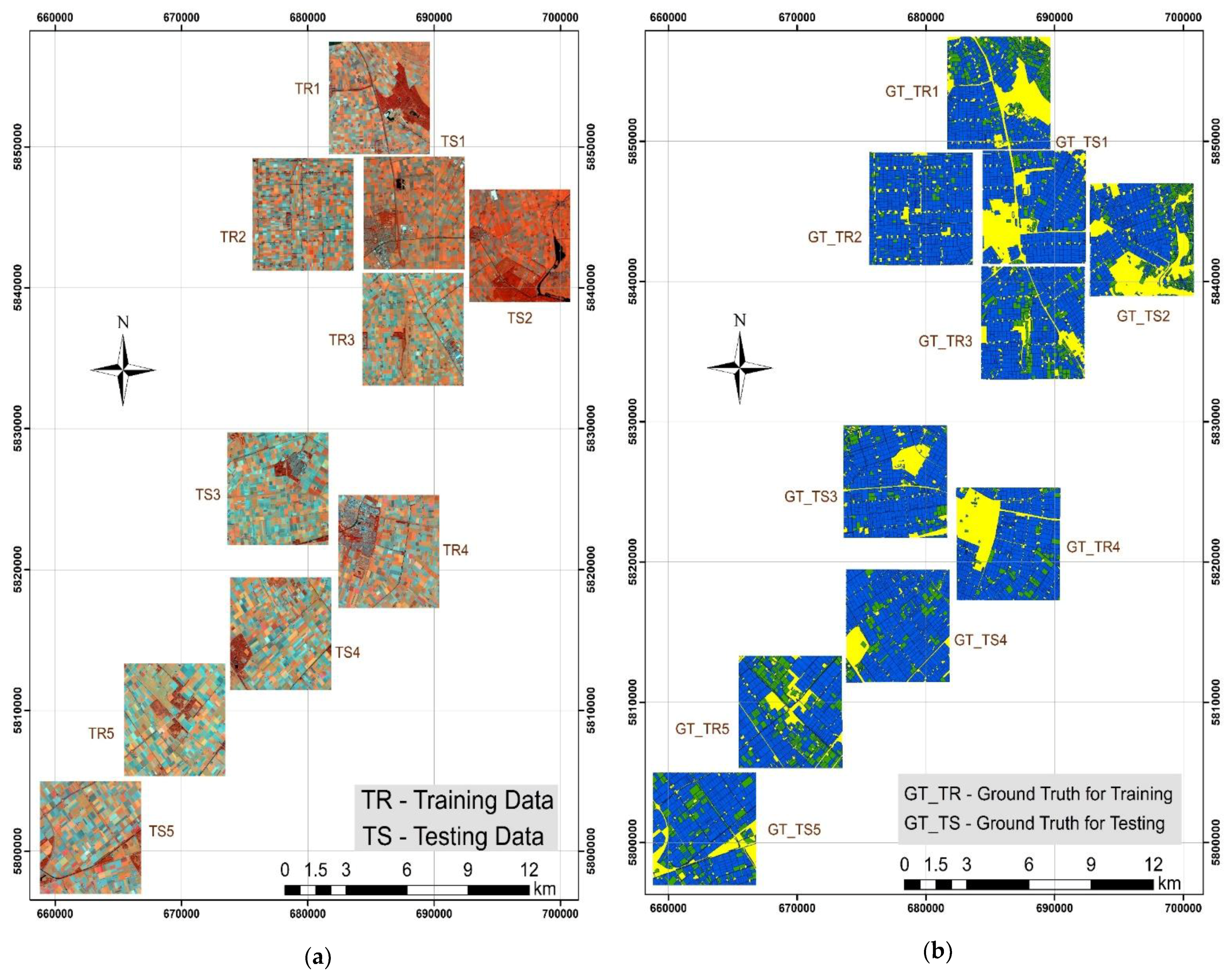
The deep learning methods developed in this study (MD-FCN and SRC-Net) are robust for detecting agricultural fields. The methods are replicable and scalable to the whole province of Flevoland. This is because the training data used for training the networks were good representative for the whole province of Flevoland. Therefore, it is feasible to produce the map over the large area such as the entire province of Flevoland. Additionally, these methods can be applied to the whole country of the Netherlands and other countries provided that enough training data is available. A challenging aspect is the processing time, especially in the training phase. In the testing phase, FCNs are computationally efficient.

5.3. Limitation of the Methods

In this study, both methods that we developed (MD-FCN and SRC-Net) are time consuming as they approximately require 2 and 4 h for MD-FCN and SRC-Net respectively to train the model from a tile of 800$\times 800$ pixels at 10 m resolution using a graphical processing unit (GPU). This is because the methods are deep as they comprised a large number of convolutional layers. Therefore, the methods need more processing power including both central processing unit (CPU) and GPU. Additionally, for training and testing a large area, a random access memory (RAM) of at least 16 GB is needed for convenience performance of processing. In addition, all methods produced fragmented boundary maps. These outputs depict that the boundary delineation problem using FCN is a challenge because the networks learn small and thin features such as lines. The limitation can be solved by deriving a hierarchical segmentation as in [4].

6. Conclusions

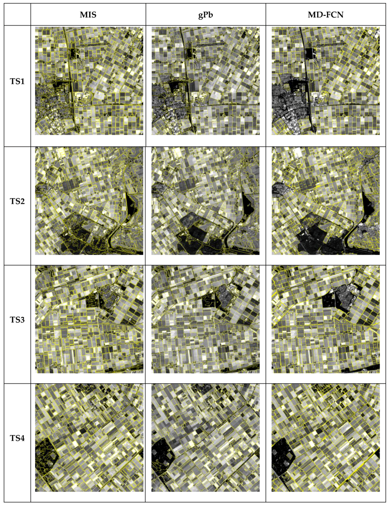
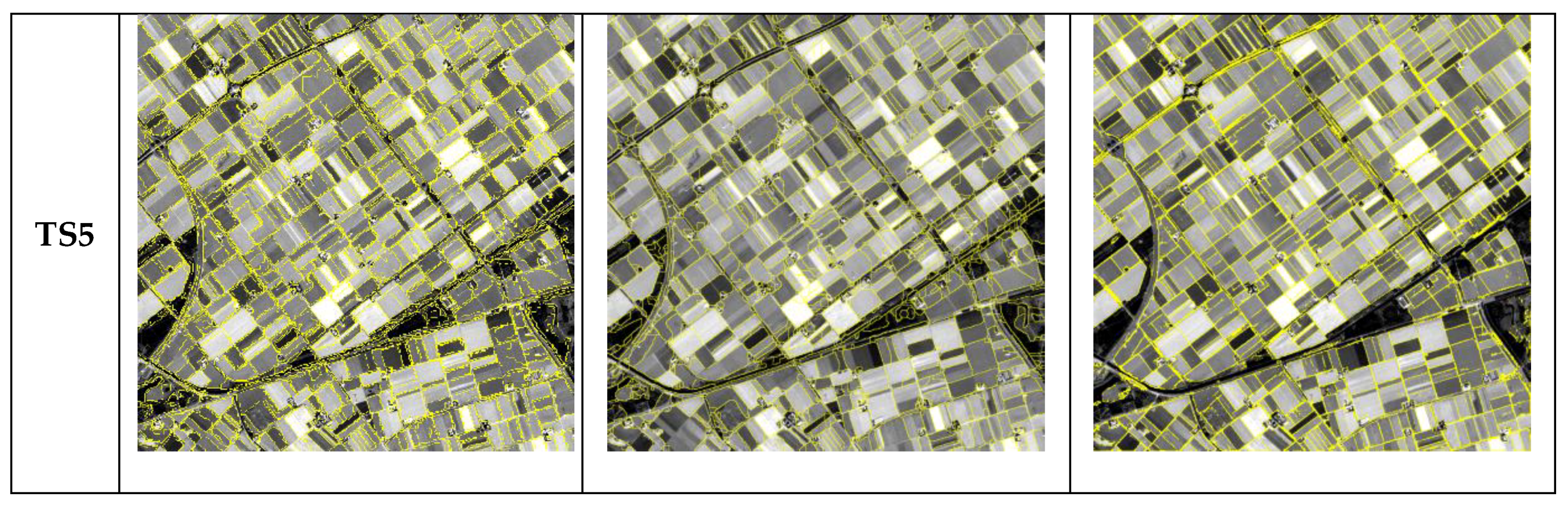
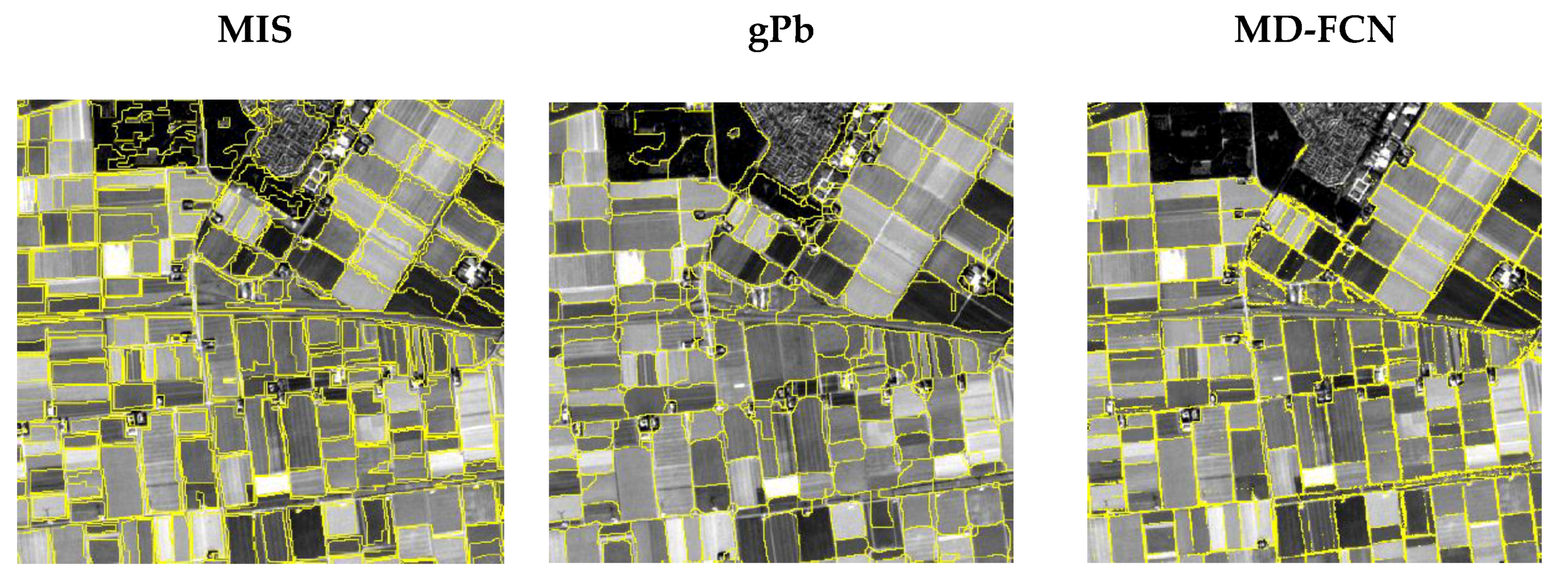
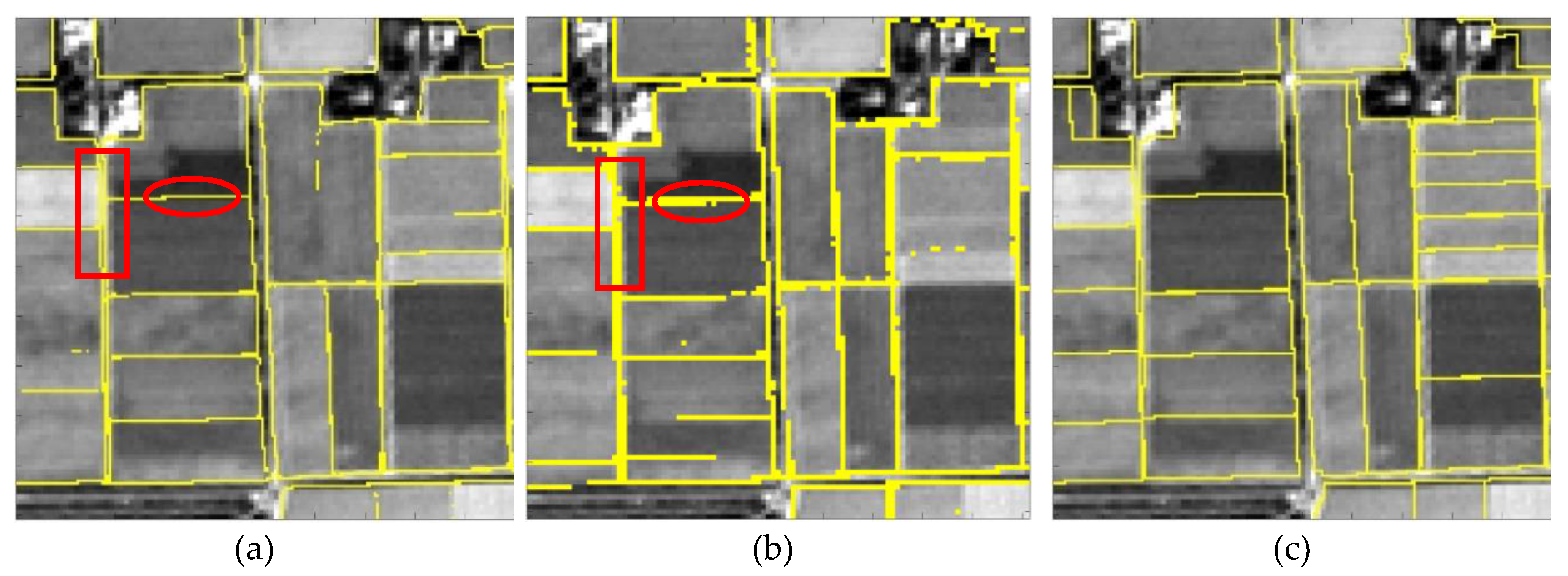
In reference to the accuracy assessment presented in Section 5.1, both MD-FCN and SRC-Net methods can be applied to detect boundaries of agricultural fields. We applied the baseline methods gPb and multiresolution image segmentation using eCognition. Based on the obtained accuracy, MD-FCN performs significantly better than the baseline methods with an increment of 31%–32% in the average F-score. This is because the MD-FCN can automatically learn discriminative spatial-contextual features from the input images and precisely generate the required outputs. Furthermore, the SRC-Net reduces the noise and increases the capability of separating different fields. The results of SRC-Net show that this network is applicable in detecting agricultural field boundaries, showing the opportunity of using open and free data of Sentinel-2 to automatically detect boundaries at 5 m resolution.

In future work, we will aim at developing the strategies to produce segmentation where fragmented boundaries are connected to obtain close contours. Additionally, we may apply the MD-FCN on study areas other than Flevoland that have irregular fields. Future work should involve the investigation of the vector format for reference data as this could increase the classification output accuracy, especially when we consider buffering the feature. This technique will allow us to include location tolerance, hence increasing the assessment accuracy.

References

1. Ji, C.Y. Delineating agricultural field boundaries from TM imagery using dyadic wavelet transforms. ISPRS J. Photogramm. Remote Sens. 1996, 51, 268–283. [Google Scholar] [CrossRef]
2. European Commission. Cap Explained. Direct Payments for Farmers 2015-2020; EU Publications: Brussels, Belgium, 2018. [Google Scholar] [CrossRef]
3. Rydberg, A.; Borgefors, G. Integrated Method for Boundary Delineation of Agricultural Fields in Multispectral Satellite Images. IEEE Trans. Geosci. Remote Sens. 2001, 39, 2514–2520. [Google Scholar] [CrossRef]
4. Persello, C.; Tolpekin, V.A.; Bergado, J.R.; de By, R.A. Delineation of agricultural fields in smallholder farms from satellite images using fully convolutional networks and combinatorial grouping. Remote Sens. Environ. 2019, 231, 111253. [Google Scholar] [CrossRef] [PubMed]
5. Sonobe, R.; Yamaya, Y.; Tani, H.; Wang, X.; Kobayashi, N.; Mochizuki, K. Crop classification from Sentinel-2-derived vegetation indices using ensemble learning. J. Appl. Remote Sens. 2018, 12, 1. [Google Scholar] [CrossRef] [Green Version]
6. Belgiu, M.; Csillik, O. Sentinel-2 Cropland Mapping Using Pixel-Based and Object-Based Time-Weighted Dynamic Time Warping Analysis. Remote Sens. Environ. 2018, 204, 509–523. [Google Scholar] [CrossRef]
7. Lebourgeois, V.; Dupuy, S.; Vintrou, É.; Ameline, M.; Butler, S.; Bégué, A. A Combined Random Forest and OBIA Classification Scheme for Mapping Smallholder Agriculture at Different Nomenclature Levels Using Multisource Data (Simulated Sentinel-2 Time Series, VHRS and DEM). Remote Sens. 2017, 9, 259. [Google Scholar] [CrossRef] [Green Version]
8. Spatial-Resolutions-Sentinel-2 MSI-User Guides-Sentinel Online. Available online: https://earth.esa.int/web/sentinel/user-guides/sentinel-2-msi/resolutions/spatial (accessed on 4 August 2019).
9. Rieke, C. Deep Learning for Instance Segmentation of Agricultural Fields. Master’s Thesis, Friedrich-Schiller-University of Jena, Jena, Germany, 2017. Available online: https://github.com/chrieke/InstanceSegmentation_Sentinel2/blob/master/thesis.pdf (accessed on 4 August 2019).
10. Turker, M.; Kok, E.H. Field-Based Sub-Boundary Extraction from Remote Sensing Imagery using Perceptual Grouping. ISPRS J. Photogramm. Remote Sens. 2013, 79, 106–121. [Google Scholar] [CrossRef]
11. Chen, B.; Qiu, F.; Wu, B.; Du, H. Image segmentation based on constrained spectral variance difference and edge penalty. Remote Sens. 2015, 7, 5980–6004. [Google Scholar] [CrossRef] [Green Version]
12. Arbeláez, P.; Maire, M.; Fowlkes, C.; Malik, J. Contour Detection and Hierarchical Image Segmentation. IEEE Trans. Pattern Anal. Mach. Intell. 2011, 33, 898–916. [Google Scholar] [CrossRef] [PubMed] [Green Version]
13. Bergado, J.R.; Persello, C.; Stein, A. Recurrent Multiresolution Convolutional Networks for VHR Image Classification. IEEE Trans. Geosci. Remote Sens. 2018, 56, 1–14. [Google Scholar] [CrossRef] [Green Version]
14. Ajami, A.; Kuffer, M.; Persello, C.; Pfeffer, K. Identifying a Slums’ Degree of Deprivation from VHR Images Using Convolutional Neural Networks. Remote Sens. 2019, 11, 1282. [Google Scholar] [CrossRef] [Green Version]
15. Xia, X.; Persello, C.; Koeva, M. Deep Fully Convolutional Networks for Cadastral Boundary Detection from UAV Images. Remote Sens. 2019, 11, 1725. [Google Scholar] [CrossRef] [Green Version]
16. Atkinson, P.M. Super-Resolution Mapping Using the Two-Point Histogram and Multi-Source Imagery. In geoENV VI—Geostatistics for Environmental Applications Dordrecht; Springer: New York, NY, USA, 2008; pp. 307–321. [Google Scholar] [CrossRef]
17. Tolpekin, V.A.; Stein, A. Quantification of the Effects of Land-Cover-Class Spectral Separability on the Accuracy of Markov-Random-Field-Based Superresolution Mapping. IEEE Trans. Geosci. Remote Sens. 2009, 47, 3283–3297. [Google Scholar] [CrossRef]
18. Heltin Genitha, C.; Vani, K. Super Resolution Mapping of Satellite Images using Hopfield Neural Networks. In Proceedings of the Recent Advances in Space Technology Services and Climate Change 2010 (RSTS & CC-2010), Chennai, India, 13–15 November 2010; IEEE: București, Romania, 2011. [Google Scholar] [CrossRef]
19. Persello, C.; Stein, A. Deep Fully Convolutional Networks for the Detection of Informal Settlements in VHR Images. IEEE Geosci. Remote Sens. Lett. 2017, 14, 2325–2329. [Google Scholar] [CrossRef]
20. Rizaldy, A.; Persello, C.; Gevaert, C.; Oude Elberink, S.; Vosselman, G. Ground and Multi-Class Classification of Airborne Laser Scanner Point Clouds Using Fully Convolutional Networks. Remote Sens. 2018, 10, 1723. [Google Scholar] [CrossRef] [Green Version]
21. Simonyan, K.; Zisserman, A. Very Deep Convolutional Networks for Large-Scale Image Recognition. Available online: http://arxiv.org/abs/1409.1556 (accessed on 4 August 2019).
22. ESA. Sen2Cor | STEP. Available online: http://step.esa.int/main/third-party-plugins-2/sen2cor/ (accessed on 1 October 2018).
23. Geo services-PDOK. Available online: https://www.pdok.nl/geo-services/-/article/basisregistratie-gewaspercelen-brp- (accessed on 17 September 2019).
24. Hijmans, R.J. Geographic Data Analysis and Modeling [R package raster version 2.8-19]. Comprehensive R Archive Network (CRAN). Available online: https://cran.r-project.org/web/packages/raster/index.html (accessed on 4 August 2019).
25. Bivand, R.; Keitt, T.; Rowlingson, B. Bindings for the “Geospatial” Data Abstraction Library [R package rgdal version 1.3-9]. Comprehensive R Archive Network (CRAN). Available online: https://cran.r-project.org/web/packages/rgdal/index.html (accessed on 4 August 2019).
26. Bivand, R.; Rundel, C. Interface to Geometry Engine-Open Source (‘GEOS’) [R package rgeos version 0.4-2]. Comprehensive R Archive Network (CRAN). Available online: https://cran.r-project.org/web/packages/rgeos/index.html (accessed on 4 August 2019).
27. Hossin, M.; Sulaiman, M.N. A Review on Evaluation Metrics for Data Classification Evaluations. Int. J. Data Min. Knowl. Manag. Process (IJDKP) 2015, 5, 1–11. [Google Scholar] [CrossRef]
28. López, V.; Fernández, A.; García, S.; Palade, V.; Herrera, F. An insight into classification with imbalanced data: Empirical results and current trends on using data intrinsic characteristics. Inf. Sci. 2013, 250, 113–141. [Google Scholar] [CrossRef]
Figure 1. General network architecture for the multiple dilation fully convolutional network (MD-FCN). Input image can be any number of channels (bands) of the same resolution. In this study, we used the Sentinel-2 band combination of the 10 m spatial resolution. The output map has the same spatial resolution as an input image. Yellow lines represent the boundaries.
Remotesensing 12 00059 g001
Figure 2. In the super-resolution semantic contour detection network (SRC-Net) architecture the input image is a band combination at the 10 m resolution and the output map containes the agricultural field boundaries (AFB) boundaries at 5 m resolution.
Remotesensing 12 00059 g002
Figure 3. Location of the tiles in Flevoland using Sentinel-2. TR represent tiles for training and TS represent tiles for testing the network (a). Ten tiles representing the reference data, five ground truth used for training represented as GT_TR, and five ground used for testing represented as GT_TS (b).
Remotesensing 12 00059 g003
Figure 4. AFB maps at 10 m resolution from Sentinel-2 image using MD-FCN (a), the circle shows the noise and rectangle shows the confusion of the parallel boundaries. (b) The ground sample distance at 10 m resolution.
Remotesensing 12 00059 g004
Figure 5. (a) The improved AFB maps at 5 m resolution from Sentinel-2 image using SRC-Net. The result shows less noise (see e.g., the red circle) and less confusion between parallel boundaries (see e.g., the red rectangle). (b) The ground sample distance at 5 m resolution obtained from RapidEye image.
Remotesensing 12 00059 g005
Figure 6. AFB maps at 10 m resolution from Sentinel-2 image using different methods. The yellow lines represent the boundaries.
Remotesensing 12 00059 g006aRemotesensing 12 00059 g006b
Figure 7. Detail of the AFB maps at 10 m resolution from Sentinel-2 image using three methods from the TS3. The yellow lines represent the boundaries.
Remotesensing 12 00059 g007
Figure 8. AFB output maps from SRC-Net (a) and output map from nearest neighbor-based resample of output of MD-FCN at 10 m resolution (b) with their reference map of 5 m resolution (c).
Remotesensing 12 00059 g008