Abstract
Information on habitat preferences is critical for the successful conservation of endangered species. For many species, especially those living in remote areas, we currently lack this information. Time and financial resources to analyze habitat use are limited. We aimed to develop a method to describe habitat preferences based on a combination of bird surveys with remotely sensed fine-scale land cover maps. We created a blended multiband remote sensing product from SPOT 6 and Landsat 8 data with a high spatial resolution. We surveyed populations of three bird species (Yellow-breasted Bunting Emberiza aureola, Ochre-rumped Bunting Emberiza yessoensis, and Black-faced Bunting Emberiza spodocephala) at a study site in the Russian Far East using hierarchical distance sampling, a survey method that allows to correct for varying detection probability. Combining the bird survey data and land cover variables from the remote sensing product allowed us to model population density as a function of environmental variables. We found that even small-scale land cover characteristics were predictable using remote sensing data with sufficient accuracy. The overall classification accuracy with pansharpened SPOT 6 data alone amounted to 71.3%. Higher accuracies were reached via the additional integration of SWIR bands (overall accuracy = 73.21%), especially for complex small-scale land cover types such as shrubby areas. This helped to reach a high accuracy in the habitat models. Abundances of the three studied bird species were closely linked to the proportion of wetland, willow shrubs, and habitat heterogeneity. Habitat requirements and population sizes of species of interest are valuable information for stakeholders and decision-makers to maximize the potential success of habitat management measures.
Keywords:
habitat preference; habitat mapping; SPOT 6; Landsat 8; downscaling; breeding bird; Emberiza; Russia 1. Introduction
Satellite remote sensing plays an increasingly important role in ecology, e.g., for estimating and monitoring biodiversity [1,2], the quantification of ecosystem services [3], and for evaluating the effectiveness of conservation interventions [1,3]. Yet, despite the rapid global decline in species richness and abundance over the past decades [4,5], a major challenge in conservation ecology is our limited knowledge on the population sizes and habitat preferences of animal species in understudied regions [6,7,8]. Here, the use of remote sensing data to predict species distributions and abundances is vital to improve large-scale biodiversity monitoring and species conservation [2,3,9].
Optical remote sensing is often suggested as a powerful tool to assist with the mapping of protected habitats and vegetation. Moreover, spaceborne remote sensing offers the opportunity to map larger areas in a systematic, repeatable, and spatially exhaustive manner [10,11]. Apart from the spatial extent of the data, its grain or spatial resolution is another relevant issue of spatial scale. Ideally, the pixel resolution of remotely sensed and considered environmental data (e.g., information on habitat features) should match to model their relationships [12]. For example, the classical multispectral configuration of Landsat-4 to Landsat-8 provides a pixel size of 30 × 30 m and an image extent of 185 × 185 km. This allows linking Landsat data to environmental data collected at a similar spatial extent and resolution. For more detailed local analyses, a higher spatial resolution of remotely sensed data is necessary [13]. Rhodes et al. [14] compared the value of field surveys and remote sensing for biodiversity assessment while using different datasets for the modelling of bird species abundances at the 1 km level. They found the resolution of the analyzed remote sensing data (>0.5 ha) to be a bottleneck for reliable models. Best results were obtained with broad land cover categories combined with information about landscape features (as hedges or single trees), both recorded in a high spatial resolution in field surveys.
In addition to spatial extent and spatial resolution, the information that can be generated from remotely sensed data is also linked to the spectral resolution and range (i.e., wavelength ranges utilized) [1]. A configuration comprising spectral bands from the visible to the near-infrared is typical for satellite sensors with a high spatial resolution as, for example, GeoEye, Ikonos, KompSat, Pleiades, QuickBird, RapidEye, or SPOT-6/7, while spectral bands in the shortwave infrared (SWIR) are usually missing. At this point, Worldview-3 (launched in 2014) is an exception with 16 multispectral bands including eight SWIR bands with a nominal pixel ground resolution of 3.7 m. The integration of SWIR bands with an adequate resolution, however, has been shown to be essential for classification purposes and the spectral discrimination of vegetation [15,16].
For birds, remote sensing data have been widely used to map their habitats, and to predict distribution and abundance (e.g., [17,18,19,20,21,22]). Remotely sensed spectral data were either used directly for modelling approaches [17] or, more commonly, indirectly by an integration of remote sensing-derived products such as land cover data [22], vegetation indices [23], or image derived textural metrics [24]. Existing studies were largely based on coarse to intermediate resolution MODIS [21,22,25] or Landsat products [20,26,27]. The majority of studies using remote sensing derived products were based on freely available spatial data, such as subregional habitat maps [28], regional cropland data layers [29], and national or global land cover data sets [30,31]. This often caused temporal mismatches between animal observations and the acquisition date of derived parameters of landscape composition or suffered from spatial mismatches due to the commonly coarse resolution of the analyzed products [25]. Associated with the resolution of these data, the studied areas were usually large and the input data rarely had a higher resolution than 30 m. Hence, small-scale landscape features, such as hedges, shrubs, and small tree stands were often not mapped, which resulted in a loss of information on habitat–species dependencies [14]. With few exceptions (harnessing SPOT-5 [32], and Worldview-2 data [33]), studies linking fine-grained habitat to spatial patterns of bird species diversity or abundance have been relying on the use of airborne observation data, such as aerial images [34,35] or LiDAR data [36,37]. A low spatial resolution of the spaceborne remote sensing data is therefore a key bottleneck, and ecologically relevant small-scale habitat features need to be considered more.
In this study, we focus on an area in the Russian Far East that hosts populations of several globally threatened bird species [38]. To identify habitat preferences and predict population sizes remote sensing data with a high spatial resolution are needed. Recent remote sensing methods offer techniques to combine fine-scale information for local approaches with the complete coverage of a larger area. These techniques include the blending of spectrally different sensor data combined with a downscaling procedure to enhance the spatial resolution of less-resolved bands [39]. Usually, reflectances acquired in bands with a fine spatial resolution are used as predictor variables to sharpen less-resolved data. All data may be acquired simultaneously with one sensor, as it is the usual case with pansharpening that aims at fusing a multispectral and a panchromatic image with the spectral resolution of the first and the spatial resolution of the second [40]. Alternatively, data may originate from different sensors with temporally close data acquisitions.
We aimed:
- to generate a multiband remote sensing product with a sufficient spatial resolution to detect small-scale landscape features; for this issue, we used data blending techniques to combine pansharpened SPOT 6 (VIS-NIR bands, 1.5 m pixel size) and Landsat-8 data, the latter providing SWIR bands with an original resolution of 30 m which were downscaled to a spatial resolution of 6 m.
- to analyze the benefit of the multiband (VIS-NIR-SWIR) product towards VIS-NIR data alone for reachable classification accuracies.
- to combine survey data of three selected breeding bird species—the “critically endangered” Yellow-breasted Bunting (Emberiza aureola), the “near threatened” Ochre-rumped Bunting (Emberiza yessoensis), and the Black-faced Bunting (Emberiza spodocephala)—with habitat information derived from the newly generated remote sensing product to model habitat preferences and population sizes.
2. Materials and Methods
2.1. Study Area
We collected field data in the Muraviovka Park for Sustainable Land Use, which was the first private nature reserve established in Russia. The park is located in the very south of the Russian Far East [38], in the Zeya-Bureya lowland next to the Amur River. The Park mainly consists of natural floodplain habitats (Figure 1). The vegetation of the Park is composed of extensive wet meadows and reeds, small forest patches, and steppe grasslands. Of the latter, the largest part has been transformed into cropland. Characteristic vegetation comprises low-growing willow species (<2 m). The Muraviovka Park harbors significant populations of multiple globally threatened species such as the Red-crowned Crane (Grus japonicus), White-naped Crane (Antigone vipio), Swinhoe’s Rail (Coturnicops exquisitus), and Oriental Stork (Ciconia boyciana) [38,41].
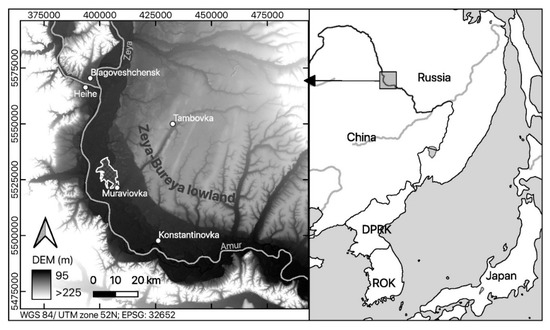
Figure 1.
Location of the study area “Muraviovka Park” within the borders of Russia (right); the floodplain of the Amur river (black) is visualized by means of the digital elevation model (SRTM, USGS) (left).
The Park covers an area of about 6450 ha. Due to the exclusion of cloud-covered parts in the satellite data at the southern border of the park site, only 6431 ha were included in our analysis.
2.2. Satellite Imagery and Processing
Commercially available SPOT 6 data (acquired on 3 September 2015) and freely available Landsat 8 (L8) Operational Land Imager (OLI) data (acquired on 4 September 2015) were used in a sharpening and blending approach to generate a multi-band product with a high spatial resolution. SPOT 6 data comprises one panchromatic band (1.5 m nominal pixel size) and four multispectral bands (blue/B, green/G, red/R, near-infrared/NIR; 6 m pixel size), all provided as top-of-atmosphere (TOA) reflectances in a “standard ortho” processing level. Landsat 8 data, unlike SPOT 6, includes two additional bands in the shortwave-infrared (SWIR-1 covering the wavelength region from 1.57 to 1.65 µm, SWIR-2 from 2.11 to 2.29 µm). Landsat 8 data set was provided as the multispectral Level-2 product with atmospherically corrected surface reflectances (SR) and a pixel size of 30 m.
To combine the advantages of both data sources, i.e., a high spatial resolution and a high spectral range including the SWIR region, we implemented a processing chain as follows: first, we masked all pixels containing clouds and cloud shades. Subsequently, the multispectral SPOT 6 bands were sharpened with the SPOT 1.5 m panchromatic band. The band-dependent spatial-detail fusion (BDSD) algorithm was selected as pansharpening approach according to the findings of Vivone et al. [40] and using their implementation provided in a MATLAB (MathWorks, Inc., Natick, MA, USA) Pansharpening toolbox (currently available from the Remote Sensing Code Library, see Acknowledgements). This step provided TOA reflectances in the B, G, R, and NIR SPOT bands, spatially sharpened to a pixel size of 1.5 m. These data were finally converted to surface reflectance with the respective L8 product based on the empirical line method [42].
A data blending approach using both SPOT 6 and Landsat 8 data was used to integrate SWIR bands in a high spatial resolution. In order to model the relationship between the high resolution SPOT (VIS-NIR, 6 m) bands and the courser resolution Landsat 8 SWIR bands (30 m), we first aggregated the SPOT four-band SR product to a pixel size of 30 m. At this level, the relationship between these data (with four predictive spectral variables) and each of the SWIR bands (as target variables) was modelled using a multiple linear regression. The obtained regression coefficients were then applied to 6 m SPOT 6 surface reflectance data to calculate artificial SWIR-1 and SWIR-2 bands with a pixel size of 6 m. As the multiple regression explained only 64% (SWIR-1) and 75% (SWIR-2) of the original variance at the 30 m level, we performed a residual correction (see e.g., [43]). Therefore, modelled SWIR bands were again resampled to 30 m and residuals between these data and the original Landsat 8 SWIR bands were calculated, resampled to 6 m spatial resolution by cubic convolution, and then added to the modelled SWIR bands at the 6 m level. A layer stack combining the pan-sharpened SPOT 6 data and the modelled (and residual-corrected) SWIR bands obtained the final product with a pixel size of 1.5 m. The downscaled SWIR bands were resampled with the nearest neighbor method to 1.5 m pixel size.
2.3. Field Survey of Breeding Birds and Collection of Land Cover Information
Field surveys were conducted from 1 May to 2 June 2017. Birds were counted at 74 points (Figure 2). Due to the inaccessibility of some areas, the sample locations were placed opportunistically along existing paths, aiming to cover all existing habitat types with a sufficient number of replicates. The exact location of the points was recorded using an Oregon 400t GPS (Garmin Ltd., Olathe, KS, USA). At each point, from 30 min before sunrise to 2 h after sunrise, we counted all territory indicating individuals of Yellow-breasted Bunting, Ochre-rumped Buntings, and Black-faced Bunting for 5 min. We recorded the perpendicular distance to the observer, in order to be able to correct for detectability varying with observer, species, vegetation, and other factors [44]. Counts were only conducted in favorable weather (no rain, no strong wind) between 04:00 and 07:00 in the morning. The breeding bird survey was repeated three times during the course of the breeding season (early May, late May/early June, late June), with changing observers (Replicate 1: author WH, Replicates 2 + 3: author AH). Distances were recorded in fixed bands of 0–10 m, 10–25 m, 25–50 m, 50–100 m, 100–250 m, and 250–500 m. A laser range finder (Bushnell Scout 1000, Overland Park, KS, USA) and topographic maps were used to calibrate the distance estimation. Inter-point distance was 500 m to avoid the multiple recording of the same individuals. Thus, there was an overlap of the 250–500 m distance bands of adjacent points. Habitat parameters that were expected to explain variation in bird abundance were recorded at each point in May and June 2017. These were moisture level, water coverage, litter cover, litter depth, and the height of shrubs and trees; assigned to predefined categories using expert knowledge. The percentage of coverage for the most common plants, aggregated to the genera level, was also recorded. Cropland was not surveyed. Reference locations of rare and thus underrepresented land cover types for the land cover mapping were additionally defined manually by visual inspection of the final high-resolution satellite product. This resulted in a total number of 557 reference locations that were available for model training and validation of the habitat mapping with remote sensing data.
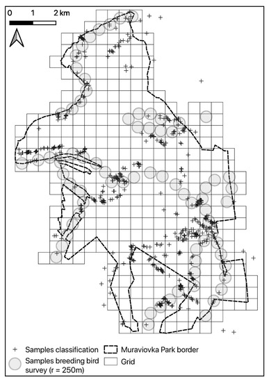
Figure 2.
An overview of the study area, with bird survey points and reference locations used for training and validation of the land cover map produced from remote sensing data.
2.4. Classification Approach for Habitat Mapping
There was a trade-off between the detail of target classes, and classification accuracy. Based on these considerations, seven land habitat classes were selected: forest, open soil, willow shrubs, hazel and clover, steppe, wetland, and water (see Table 1).

Table 1.
Description of habitat classes and habitat class-wise representation of pixels and polygons used for model training and validation.
For the extraction of spectral characteristics of the defined habitat classes, we overlaid the recorded coordinates of points where land cover ground truthing data was collected with the high-resolution satellite product. Using R [45] package raster [46], we extracted all pixel values within a buffer with a radius of 1.5 m around the point coordinates. The preparation of the calibration and test sets (60% to 40% split) was done by means of the cLHS (conditioned Latin hypercube sampling) algorithm, implemented in the R package clhs [47]. In contrast to random sampling, cLHS allows for a full statistical coverage of the data points in the n-dimensional spectral space [48], which has been shown to result in increased and more robust classification accuracies [16]. To guarantee the independence of the training and validation data sets we ensured that pixels originating from polygons used in the training data were not allowed in the test data.
For the spectral classification of the habitat types we utilized the nonparametric Random Forest classifier [49], which has been found highly valuable for vegetation discrimination based on multispectral image data [50,51,52]. The classification was conducted using the R package randomForest [53]. Random Forest is characterized by its ability to handle large numbers of correlated and even noisy predictor variables [49,50]. It is an ensemble classifier, constructing a large number of uncorrelated binary decision trees, stepwise separating the samples into more and more homogenous groups [54]. Therefore, each tree is generated using a bootstrapping method that randomly selects samples with replacement [49,54]. The remaining samples, approximately 37% of the total sample size, are referred to as OOB (out-of-bag) data [55]. Both, the number of randomly chosen predictors tested for their suitability to split a node and the number of created trees are user-defined. To estimate the accuracy (OOB-error), each tree classifies its OOB data. The membership of each sample to a certain class is then determined by the majority vote of all trees [56], which makes the classifier less prone to overfitting. The number of trees was set to 5000 to ensure the OOB error term converges. For the number of predictors, we kept the default value (square root of total number of predictors (n = 2)). To evaluate classifier stability, Random Forest models were trained and tested on 25 different calibration sets and subsequently validated with 25 different test sets. Each of these sets was defined with cLHS, as it does not provide one unique solution in the split of calibration and validation data [50]. Classification accuracies were evaluated based on contingency tables, derived from classified datasets and reference data. Here, we present the most common measures of accuracy: the overall accuracy (OAA, percentage of correctly classified samples); the user’s accuracy (UA, class-wise percentage of correctly classified samples); the producer’s accuracy (PA, the percentage of samples labelled correctly within a certain class) and the kappa coefficient (Kappa, overall accuracy corrected from chance correspondences).
2.5. Modelling Drivers of Bird Abundance
Monitoring the abundance and distribution of mobile organisms, such as birds, remains challenging due to imperfect detection in the field [57]. In order to obtain less biased abundance estimates we used distance sampling [57] that corrects for a varying detection probability (δ, detection function). For estimating the population density, we used the extended hierarchical distance sampling model as proposed by Chandler et al. [58], made available in the R package unmarked [59] as function gdistsamp. It allows including environmental covariates for the modelling of abundances (λ), and relaxes the assumption of geographic closure, i.e., no immigration or emigration during the survey period, by introducing a parameter for temporal population dynamics arising from organism mobility (φ, availability).
Habitat proportions derived from the high-resolution habitat map and habitat heterogeneity, represented by Shannon’s diversity index (H) [60], with pi being the relative proportion of the land cover class i and S being the total number of land cover types per grid cell (see Equation (1)), were fitted as abundance (λ)-covariates to calculate habitat-specific species abundances.
The daytime of field data acquisition and the survey replicate (Replicates 1–3) were fitted as availability (φ)-covariates to correct for temporal and inner-seasonal variation of species availability. Additionally, observer was fitted as a detection (δ)-covariate to allow for varying detection skills among observers. A half-normal detection function was used in all models. We used the Akaike information criterion (AIC) to compare model fit and complexity of various candidate models [61]. First, two null models (intercept only, no covariates), were compared using either a Poisson distribution for the abundance component (λ) or a negative binomial distribution (including the dispersion parameter α). Second, single component models were fitted, considering all land cover types and habitat diversity as covariate for the abundance component (λ). We furthermore included quadratic effects for each covariate. Additionally, single effect models for the detection component (δ) and the availability (φ) component were fitted, resulting in 22 single effect models in total for each species. Due to the low availability of Yellow-breasted Bunting in the survey period of the first observer, the detection (δ)-covariate was excluded from models for this species. Finally, important covariates for each model component, as indicated by AIC, were selected to fit models with combined effects. To this end, only positive effects on abundance (λ) were considered to provide parsimonious and meaningful models of habitat preferences of the target species.
Parametric bootstrapping was used to evaluate the goodness-of-fit for the best model for each bird species [28,62]. We used the final model to simulate 1000 datasets and refit the model to this data to compute fit statistics, respectively. In a subsequent step, we compared the values of fit statistics for the observed data to the modelled distribution of the simulated data using the p-value of the Freeman–Tukey test which requires no pooling of cells with small values in contrast to the X2 test [28,62]. A good model fit is indicated by a low deviation of the observed distribution from the modelled distribution, with a p-value excluding significant differences (0.5 in the best case) [63]. The models which fitted the data best were finally selected to predict the abundance of the target species based on the classified habitat proportion per 500 m grid cell (Figure 2), accounting for differences in area between the point transects and grid cells by linear interpolation. Total population sizes were estimated by summing up the predicted abundances over all grid cells.
3. Results
3.1. Comparison of Accuracies Achieved in the Habitat Classification
We used two different datasets for the Random Forest classification approach: pan-sharpened SPOT-6 VIS-NIR data alone and combined with sharpened SWIR bands from Landsat-8. The first dataset provided an OAA of 71.3% (mean value obtained in all classification runs) for the seven habitat classes defined according to Table 1. A slightly better OAA (73.2%) was achieved in the classification of the stacked VIS-NIR-SWIR data (see Figure 3). The benefit of including SWIR data increased with an increasing number of considered habitat types (see Figure S1). Nevertheless, accuracies generally dropped by as the number of labelled classes was decreased and amounted to 62.4% for 24 classes with VIS-NIR-SWIR data (54.9% with VIS-NIR alone). A class-wise analysis of achieved accuracies indicated marked improvements with SWIR bands especially for classes with small-scale features (hazel and clover, willow shrubs; Figure 3). Results were different for “open soil” and ”steppe”, for which VIS-NIR data slightly outperformed full range VIS-NIR-SWIR data. The best VIS-NIR-SWIR model out of 25 repetitions achieved 76.7% OAA (Kappa = 67.8). This model was thus selected for the final habitat mapping (Figure 4). On the level of single habitat types, highest user and producer accuracies were achieved for the classes ‘Open Soil’, ‘Water’, and ‘Wetland’. Lowest class specific accuracies were achieved for ‘Shrubs: willow’. The class ‘Wetland’ as the dominant habitat type in our study site caused most classification errors, leading to reduced user and/or producer accuracies especially for the classes ‘Forest’, ‘Shrub: willow’ and ‘Steppe’ (see Table 2). The spatial distribution of classified land cover classes is shown in the resulting habitat map (Figure 4).
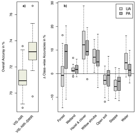
Figure 3.
Comparison of (a) overall accuracies for the VIS-NIR and VIS-NIR-SWIR data sets as obtained for test data unseen in the training (25 repetitions) and (b) class-wise difference for User (UA) and Producer Accuracy (PA) between VIS-NIR-SWIR and VIS-NIR (positive values indicate superior results for the VIS-NIR-SWIR datasets).
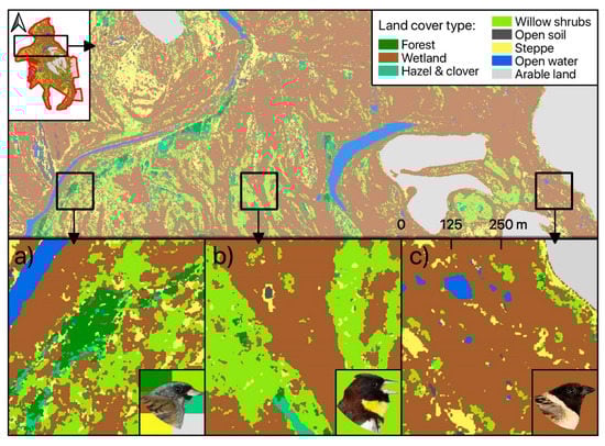
Figure 4.
Habitat map resulting from high-resolution VIS-NIR-SWIR remote sensing product. Proportions of habitat class per 25 ha grid cell were used as covariates in the distance-sampling models for each species. Exemplary representation of favored habitat types as indicated by the bird image background color are shown for Black-faced Bunting (a), Yellow-breasted Bunting (b), and Ochre-rumped Bunting (c).
Table 2.
Contingency table and accuracies (UA = user accuracy, PA = producer accuracy, OAA = overall accuracy, all accuracies given in %) achieved for the best classification model, which was afterwards used for the habitat mapping of the entire study area.
3.2. Determinants of Bird Abundance
In total, 148 individuals of the Yellow-breasted Bunting, 144 individuals of the Ochre-rumped Bunting, and 214 individuals of the Black-faced Bunting were detected during our bird survey. Details on model selection results obtained from the bird species-specific hierarchical distance sampling models can be found in the Supplementary Material (Table S1). As indicated by lower AIC values, models fitted using a negative binomial distribution generally received more support than those that were fitted using a Poisson distribution. The best supported model for the Yellow-breasted Bunting (AIC = 623.2) suggested that abundance was significantly positively related to the share of willow shrubs (β = 0.30, SE = 0.140, p = 0.034). The most supported model for the Ochre-rumped Bunting (AIC = 671.6) suggested that abundance was positively related to percentage wetland (β = 0.36, SE = 0.175, p = 0.041). The best supported model for Black-faced Bunting (AIC = 971.0) indicated that abundance was positively related to habitat heterogeneity, represented by the Shannon index (β = 0.24, SE = 0.095, p = 0.012). Confidence limits for Yellow-breasted Bunting and Ochre-rumped Bunting showed an increased uncertainty of the predicted abundance towards higher proportions of the land cover type (Figure 5). Including seasonality (expressed as survey round) was found to improve model performance for Yellow-breasted Bunting (Table 3). Accounting for time of day yielded no improvement for the best supported models for the respective species.
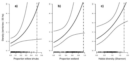
Figure 5.
Response curves (including 95% confidence limits) from the models with the lowest AIC showing the predicted density per 25 ha grid cell as a function of selected land cover covariates for (a) Yellow-breasted Bunting, (b) Ochre-rumped Bunting, and (c) Black-faced Bunting. The inner tick marks on the x-axis indicate observed values at the sample points. Dashed lines indicate maxima of observed values at the sample points.
Table 3.
Parameter estimations from the Distance-Sampling model with the lowest Akaike information criterion (AIC), for all species; standard errors are given in brackets; significance levels for p < 0.05, p < 0.01, and p < 0.001 are denoted with asterisks.
The goodness-of-fit statistics for model evaluation obtained by parametric bootstrapping suggested that all species-specific models fitted the data well with all p-values obtained from Freeman–Tukey test being close to 0.5 (Yellow-breasted Bunting = 0.64, Ochre-rumped Bunting = 0.53, Black-faced Bunting = 0.55).
Based on the retrieved results, different habitat situations can be paralleled with species abundances. Near the Amur river, in the north-western part of the study area, there was a small-scale mixture of different habitat types and high portions of willow shrub habitats, considered to be highly appropriate for the species Black-faced Bunting (a) and Yellow-breasted Bunting (b). The Ochre-rumped Bunting (c) preferred more open areas dominated by wetland e.g., in the north-eastern part of study area. The predicted species-specific abundances per grid cell (Figure 6) coincided well with the spatial patterns of the habitat types found to be important in the modelling procedure. For the entire study area, the total population size estimates (95% confidence limits in brackets) based on the best models and the complete habitat map for each species were 706 (415–1249) territories for Yellow-breasted Bunting, 1445 (756–2855) territories for Ochre-rumped Bunting, and 1282 (928–1787) territories for Black-faced Bunting.
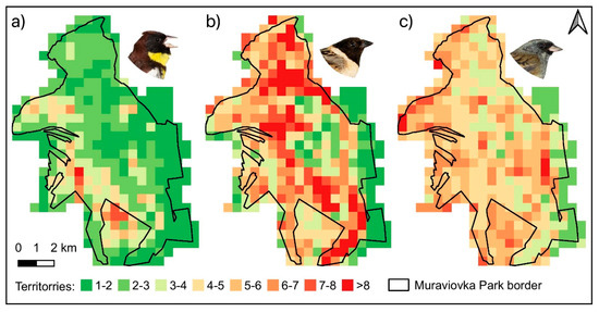
Figure 6.
Predicted abundances per grid cell (territories/25 ha) from the models receiving the most support. The Yellow-breasted Bunting model included percentage of willow shrubs as abundance effect (a), the Ochre-rumped Bunting model included percentage of wetland as abundance effect (b), and the Black-faced Bunting model included the Shannon’s diversity index as abundance effect (c).
4. Discussion
In this study we aimed at evaluating the ability of a high-resolution remote sensing product with a full range spectral band suite (VIS-NIR-SWIR, based on SPOT 6 and Landsat 8 data) to map fine scale habitat characteristics at a large spatial extent, in comparison to the sole use of SPOT 6 data. In addition, we intended to identify suitable habitats for endangered bird species in a floodplain ecosystem and to predict their population sizes using hierarchical distance sampling models informed by the remote sensing derived habitat structure.
4.1. Habitat Mapping
Classification accuracies of small-scale habitat structures such as shrubs, small forest fragments, and small water streams improved when using full range spectral data instead of VIS-NIR data alone, given a sufficient spatial resolution. These findings are in line with those of Naegeli de Torres et al. [43], where RapidEye images were combined with Landsat 5 SWIR bands (downscaled to 5 m spatial resolution) to map vegetation elements and erosion features of pastures at a very high spatial resolution. In our study, the benefit of adding SWIR bands to the remote sensing data to discriminate different vegetation types increased with the number of classes considered in the classification process. Further improvements of classification results may be expected when time series of remote sensing data are used instead of single date imagery, e.g., by capturing phenological variation [16,64]. The habitat type wetland, the most dominant habitat type at the Muraviovka Park, caused most misclassification, especially with forest, willow shrubs, and steppe. Grassland plant species also occur in forest understories and steppe. Hence, a separation of these classes based only on spectral image characteristics remains challenging. Furthermore, it could be beneficial to additionally include remotely sensed stand structure information, as e.g., obtained from LiDAR data [23,65]. The recently launched (Dec. 2018) GEDI mission (NASA, USA), for example, provides data with a relatively high spatial resolution of 25 m, but does not provide the level of detail as required in this study.
4.2. Species Specific Habitat Preferences
The applied modeling framework was based on the distance-sampling model presented by Chandler et al. [58], but additionally included bird count data from repeated surveys as φ-covariate and corrected for the detection skills of the observer (δ-covariate). The resulting hierarchical model thus enabled us to analyze spatially and temporally replicated counts of bird observations and provided spatially explicit estimates of density as a function of environmental factors. As such, we were able to evaluate how changes in such covariates could affect the population densities and habitat specific abundances. Since the applied hierarchical distance-sampling models were solely based on remotely sensed habitat characteristics, the excellent fit statistics for all three bird species models indicated remote sensing to be a valuable tool to derive habitat preferences for bird species at the local scale. Although there have been only few studies on the habitat preferences of the birds under study (as e.g., [66]), previous studies on other birds living in grassland dominated habitats have shown that these birds prefer territorial sites with a particular habitat structure [67]. The fact that the proportion of willow shrubs and wetland as well as habitat heterogeneity, the latter indicated by the Shannon index, showed the strongest relationship to species-specific abundances, suggest that small scale habitat suitability is driven by local, fine-grained habitat conditions [68]. The difficulty of finding an effect of habitat type on the abundance of Black-faced Bunting might be explained by its preference towards heterogeneous habitats, which could mirror its flexibility with regard to the selection of nest sites [66]. Mikami and Kawata [67] found a preference of Ochre-rumped Buntings towards habitats with low growing reeds and tall monocotyledons others than reed.
We are aware that the design of the breeding bird survey has some limitations, and might introduce some bias in the estimation of species abundances. Bias might also arise e.g., from double counting birds situated in the outer sampling corridors. The nonrandom sampling might also lead to an overrepresentation of certain habitat types in the sample. Detection probability might vary by habitat type. We assumed constant detectability across habitat type, since accounting for this is unreasonable as the covariate affects abundance and detection at the same time [28]. However, as our study site is an open landscape, we believe that the overall effect of habitat type on detection is low. The temporal discrepancy between the acquisition of the remote sensing data and the bird count data, which was caused by the unavailability of cloud free remote sensing data for the survey period, might also be a potential source of error. As the survey of breeding birds and collection of land cover information used for habitat mapping were undertaken simultaneously, we were able to ensure that no pronounced changes in land cover were detectable in the study area between 2015 and 2017. The land cover type “cropland” being more frequent subject to changes of land use and land cover was thus excluded from our analysis.
4.3. Management Implications
The predicted total numbers of 706, 1445, and 1282 territories for Yellow-breasted Bunting, Ochre-rumped Bunting, and Black-faced Bunting, respectively, at the Muraviovka Park provide a reliable baseline for further population monitoring. This is especially important in the light of the alarming population decline of the Yellow-breasted Bunting [69] and the resulting upgrade to the status “critically endangered” according to the IUCN Red List [70] in 2017. For the Ochre-rumped Bunting, the global population size was estimated as 6000–15,000 individuals [71]. Given the fact that we predicted 1445 territories (which equates to 2890 adult individuals), Muraviovka Park would harbor a large share of the global population of this species. As the breeding population in the Amur region is not included in the BirdLife range map for this species [71], it seems likely that the global population of the Ochre-rumped Bunting is significantly larger than the BirdLife estimate. Our results demonstrate that the floodplains of Muraviovka Park provide large areas of sufficient breeding ground, especially for the Ochre-rumped Bunting and the Black-faced Bunting, among many others [38]. Overall, monitoring protected areas and their surroundings is essential given their vulnerability to anthropogenic pressures, including those associated to climate change, fires, and agriculture [72,73]. Our presented framework could furthermore be used to estimate population sizes for larger areas, to get a better understanding of the current situation for endangered taxa such as the Yellow-breasted Bunting.
5. Conclusions
The value of remote sensing satellite data for habitat mapping increases with its spatial resolution (for the detection of fine-scale habitat structures) and the covered spectral range. Full range satellite data with a fine spatial resolution are still a bottleneck for mapping approaches, but data blending can provide improved image products to fill this gap. SWIR data were found to contribute to a successful spectral mapping of small-scaled vegetation attributes such as hazel and willow shrubs, where the latter was found to be a strong determinant to predict densities of the critically endangered Yellow-breasted Bunting. We showed that remote sensing can play a key role in establishing baselines of the extent, condition, and also the change of habitats and associated species diversity. The direct link between ecologically meaningful habitat characteristics and species abundances may be of great value to reveal more general ecological strategies of certain taxa, for example to identify habitat generalists and specialists. In this way, important information for stakeholders and decision-makers on the habitat requirements of species of interest may be provided to maximize the potential success of habitat management measures.
Supplementary Materials
The following are available online at https://www.mdpi.com/2072-4292/12/1/38/s1, Figure S1: Achieved overall accuracies for the classification of different aggregation levels for land cover classes, VIS-NIR (SPOT6) compared to the multi-band VIS-NIR-SWIR product. Figure S2: Scheme explaining the aggregation of land cover types used for the mapping with remote sensing data. Table S1: AIC values as achieved in model selection.
Author Contributions
A.H., M.V. and R.R. designed the experiment with input from W.H. and J.K., A.H. and W.H. had the initial idea for the study and collected the field data. A.H., R.R. and M.V. processed and analyzed the remote sensing data; distance sampling was performed by A.H., R.R. and J.K. R.R., A.H. and M.V. wrote the manuscript with input from J.K. and W.H. All authors contributed to the final text and helped with editing. All authors have read and agreed to the published version of the manuscript.
Funding
The fieldwork at Muraviovka Park in 2017 was supported by grants of the German Ornithologists´ Society (DO-G), the Mohamed bin Zayed Species Conservation Fund, and tier3 solutions GmbH awarded to WH.
Acknowledgments
We would like to thank the numerous helpers from the Amur Bird Project (www.amurbirding.blogspot.com) and the Muraviovka Park for supporting our fieldwork. We acknowledge support from the German Research Foundation (DFG) and Leipzig University within the program of Open Access Publishing. We used the Pansharpening Toolbox that appears in Vivone et al., 2015. The Matlab toolbox is currently available from the Remote Sensing Code Library (RSCL) as a free online registry of software codes (https://rscl-grss.org/coderecord.php?id=541).
Conflicts of Interest
The authors declare no conflict of interest. The funders had no role in the design of the study; in the collection, analyses, or interpretation of data; in the writing of the manuscript, or in the decision to publish the results.
References
- Turner, W.; Spector, S.; Gardiner, N.; Fladeland, M.; Sterling, E.; Steininger, M. Remote sensing for biodiversity science and conservation. Trends Ecol. Evol. 2003, 18, 306–314. [Google Scholar] [CrossRef]
- Kissling, W.D.; Ahumada, J.A.; Bowser, A.; Fernandez, M.; Fernández, N.; García, E.A.; Guralnick, R.P.; Isaac, N.J.B.; Kelling, S.; Los, W.; et al. Building essential biodiversity variables (EBVs) of species distribution and abundance at a global scale. Biol. Rev. Camb. Philos. Soc. 2018, 93, 600–625. [Google Scholar] [CrossRef] [PubMed]
- Rose, R.A.; Byler, D.; Eastman, J.R.; Fleishman, E.; Geller, G.; Goetz, S.; Guild, L.; Hamilton, H.; Hansen, M.; Headley, R.; et al. Ten ways remote sensing can contribute to conservation. Conserv. Biol. 2015, 29, 350–359. [Google Scholar] [CrossRef] [PubMed]
- Studds, C.E.; Kendall, B.E.; Murray, N.J.; Wilson, H.B.; Rogers, D.I.; Clemens, R.S.; Gosbell, K.; Hassell, C.J.; Jessop, R.; Melville, D.S.; et al. Rapid population decline in migratory shorebirds relying on Yellow Sea tidal mudflats as stopover sites. Nat. Commun. 2017, 8, 14895. [Google Scholar] [CrossRef] [PubMed]
- Barnosky, A.D.; Matzke, N.; Tomiya, S.; Wogan, G.O.U.; Swartz, B.; Quental, T.B.; Marshall, C.; McGuire, J.L.; Lindsey, E.L.; Maguire, K.C.; et al. Has the Earth’s sixth mass extinction already arrived? Nature 2011, 471, 51–57. [Google Scholar] [CrossRef] [PubMed]
- Boakes, E.H.; McGowan, P.J.K.; Fuller, R.A.; Chang-qing, D.; Clark, N.E.; O’Connor, K.; Mace, G.M. Distorted views of biodiversity: Spatial and temporal bias in species occurrence data. PLoS Biol. 2010, 8, e1000385. [Google Scholar] [CrossRef] [PubMed]
- Isaac, N.J.B.; Pocock, M.J.O. Bias and information in biological records. Biol. J. Linn. Soc. Lond. 2015, 115, 522–531. [Google Scholar] [CrossRef]
- Davis, S.K. Area sensitivity in grassland Passerines: Effects of patch size, patch shape, and vegetation structure on bird abundance and occurrence in Southern Saskatchewan. Ecology 2004, 121, 1130. [Google Scholar] [CrossRef]
- He, K.S.; Bradley, B.A.; Cord, A.F.; Rocchini, D.; Tuanmu, M.-N.; Schmidtlein, S.; Turner, W.; Wegmann, M.; Pettorelli, N. Will remote sensing shape the next generation of species distribution models? Remote Sens. Ecol. Conserv. 2015, 1, 4–18. [Google Scholar] [CrossRef]
- Duro, D.C.; Coops, N.C.; Wulder, M.A.; Han, T. Development of a large area biodiversity monitoring system driven by remote sensing. Prog. Phys. Geogr. 2007, 31, 235–260. [Google Scholar] [CrossRef]
- Haest, B.; Vanden Borre, J.; Spanhove, T.; Thoonen, G.; Delalieux, S.; Kooistra, L.; Mücher, C.; Paelinckx, D.; Scheunders, P.; Kempeneers, P. Habitat Mapping and Quality Assessment of NATURA 2000 heathland using airborne imaging spectroscopy. Remote Sens. 2017, 9, 266. [Google Scholar] [CrossRef]
- Elith, J.; Leathwick, J.R. Species distribution models: Ecological explanation and prediction across space and time. Ann. Rev. Ecol. Evol. Syst. 2009, 40, 677–697. [Google Scholar] [CrossRef]
- Wulder, M.A.; Hall, R.J.; Coops, N.C.; Franklin, S.E. High spatial resolution remotely sensed data for ecosystem characterization. BioScience 2004, 54, 511–521. [Google Scholar] [CrossRef]
- Rhodes, C.J.; Henrys, P.; Siriwardena, G.M.; Whittingham, M.J.; Norton, L.R. The relative value of field survey and remote sensing for biodiversity assessment. Methods Ecol. Evol. 2015, 6, 772–781. [Google Scholar] [CrossRef]
- Alonzo, M.; Bookhagen, B.; Roberts, D.A. Urban tree species mapping using hyperspectral and lidar data fusion. Remote Sens. Environ. 2014, 148, 70–83. [Google Scholar] [CrossRef]
- Richter, R.; Reu, B.; Wirth, C.; Doktor, D.; Vohland, M. The use of airborne hyperspectral data for tree species classification in a species-rich Central European forest area. Int. J. Appl. Earth Obs. 2016, 52, 464–474. [Google Scholar] [CrossRef]
- Hepinstall, J.A.; Sader, S.A. Using Bayesian statistics, Thematic Mapper satellite imagery, and breeding bird survey data to model bird species probability of occurrence in Maine. Photogramm. Eng. Remote Sens. 1997, 63, 1231–1237. [Google Scholar]
- Homer, C.G.; Edwards, T.C.; Ramsey, R.D.; Price, K.P. Use of remote-sensing methods in modeling Sage Grouse winter habitat. J. Wild. Mgmt. 1993, 57, 78–84. [Google Scholar] [CrossRef]
- Miller, K.V.; Conroy, M.J. Spot satellite imagery for mapping Kirtlands Warbler wintering habitat in the Bahamas. Wildl. Soc. Bull. 1990, 18, 252–257. [Google Scholar]
- Dronova, I.; Beissinger, S.; Burnham, J.; Gong, P. Landscape-Level Associations of Wintering Waterbird Diversity and Abundance from Remotely Sensed Wetland Characteristics of Poyang Lake. Remote Sens. 2016, 8, 462. [Google Scholar] [CrossRef]
- Macías-Duarte, A.; Panjabi, A.O.; Pool, D.B.; Ruvalcaba-Ortega, I.; Levandoski, G.J. Fall vegetative cover and summer precipitation predict abundance of wintering grassland birds across the Chihuahuan desert. J. Arid Environ. 2018, 156, 41–49. [Google Scholar] [CrossRef]
- Coops, N.C.; Bolton, D.K.; Hobi, M.L.; Radeloff, V.C. Untangling multiple species richness hypothesis globally using remote sensing habitat indices. Ecol. Indic. 2019, 107, 105567. [Google Scholar] [CrossRef]
- Goetz, S.J.; Steinberg, D.; Betts, M.G.; Holmes, R.T.; Doran, P.J.; Dubayah, R.; Hofton, M. Lidar remote sensing variables predict breeding habitat of a Neotropical migrant bird. Ecology 2010, 91, 1569–1576. [Google Scholar] [CrossRef] [PubMed]
- Bellis, L.M.; Pidgeon, A.M.; Radeloff, V.C.; St-Louis, V.; Navarro, J.L.; Martella, M.B. Modeling habitat suitability for Greater Rheas based on satellite image texture. Ecol. Appl. 2008, 18, 1956–1966. [Google Scholar] [CrossRef] [PubMed]
- Butler, M.J.; Sesnie, S.E.; Timmer, J.M.; Harris, G. Integrating land surface phenology with cluster density and size improves spatially explicit models of animal density. Remote Sens. Environ. 2017, 199, 51–62. [Google Scholar] [CrossRef]
- Bino, G.; Levin, N.; Darawshi, S.; van der Hal, N.; Reich-Solomon, A.; Kark, S. Accurate prediction of bird species richness patterns in an urban environment using Landsat-derived NDVI and spectral unmixing. BioScience 2008, 29, 3675–3700. [Google Scholar] [CrossRef]
- Buchanan, G.; Pearce-Higgins, J.; Grant, M.; Robertson, D.; Waterhouse, T. Characterization of moorland vegetation and the prediction of bird abundance using remote sensing. J. Biogeogr. 2005, 32, 697–707. [Google Scholar] [CrossRef]
- Sillett, T.S.; Chandler, R.B.; Royle, J.A.; Kery, M.; Morrison, S.A. Hierarchical distance-sampling models to estimate population size and habitat-specific abundance of an island endemic. Ecol. Appl. 2012, 22, 1997–2006. [Google Scholar] [CrossRef]
- Timmer, J.M.; Butler, M.J.; Ballard, W.B.; Boal, C.W.; Whitlaw, H.A. Spatially explicit modeling of lesser prairie-chicken lek density in Texas. J. Wild. Mgmt. 2014, 78, 142–152. [Google Scholar] [CrossRef]
- Blank, P.J. Northern bobwhite response to Conservation Reserve Program habitat and landscape attributes. J. Wild. Mgmt. 2013, 77, 68–74. [Google Scholar] [CrossRef]
- Koshkin, M.A.; Burnside, R.J.; Collar, N.J.; Guilherme, J.L.; Showler, D.A.; Dolman, P.M. Effects of habitat and land use on breeding season density of male Asian Houbara Chlamydotis macqueenii. J. Ornithol. 2016, 157, 811–823. [Google Scholar] [CrossRef]
- Besnard, A.G.; Davranche, A.; Maugenest, S.; Bouzillé, J.B.; Vian, A.; Secondi, J. Vegetation maps based on remote sensing are informative predictors of habitat selection of grassland birds across a wetness gradient. Ecol. Indic. 2015, 58, 47–54. [Google Scholar] [CrossRef]
- Mairota, P.; Cafarelli, B.; Labadessa, R.; Lovergine, F.; Tarantino, C.; Lucas, R.M.; Nagendra, H.; Didham, R.K. Very high resolution Earth observation features for monitoring plant and animal community structure across multiple spatial scales in protected areas. Int. J. Appl. Earth Obs. 2015, 37, 100–105. [Google Scholar] [CrossRef]
- St-Louis, V.; Pidgeon, A.M.; Radeloff, V.C.; Hawbaker, T.J.; Clayton, M.K. High-resolution image texture as a predictor of bird species richness. Remote Sens. Environ. 2006, 105, 299–312. [Google Scholar] [CrossRef]
- Sesnie, S.E.; Mueller, J.M.; Lehnen, S.E.; Rowin, S.M.; Reidy, J.L.; Thompson, F.R. Airborne laser altimetry and multispectral imagery for modeling Golden-cheeked Warbler (Setophaga chrysoparia) density. Ecosphere 2016, 7, 430. [Google Scholar] [CrossRef]
- Boelman, N.T.; Asner, G.P.; Hart, P.J.; Martin, R.E. Multi-trophic invasion resistance in Hawaii: Bioacoustics, field surveys, and airborne remote sensing. Ecol. Appl. 2007, 17, 2137–2144. [Google Scholar] [CrossRef]
- Kortmann, M.; Heurich, M.; Latifi, H.; Rösner, S.; Seidl, R.; Müller, J.; Thorn, S. Forest structure following natural disturbances and early succession provides habitat for two avian flagship species, capercaillie (Tetrao urogallus) and hazel grouse (Tetrastes bonasia). Biol. Conserv. 2018, 226, 81–91. [Google Scholar] [CrossRef]
- Heim, W.; Smirenski, S.M. The importance of Muraviovka Park / Far East Russia for endangered bird species on regional, national and international scale based on observations from 2011–2016. Forktail 2017, 33, 77–83. [Google Scholar]
- Atkinson, P.M. Downscaling in remote sensing. Int. J. Appl. Earth Obs. 2013, 22, 106–114. [Google Scholar] [CrossRef]
- Vivone, G.; Alparone, L.; Chanussot, J.; Dalla Mura, M.; Garzelli, A.; Licciardi, G.A.; Restaino, R.; Wald, L. A critical comparison among pansharpening algorithms. IEEE Trans. Geosci. Remote Sens. 2015, 53, 2565–2586. [Google Scholar] [CrossRef]
- Heim, W.; Trense, D.; Heim, A.; Kamp, J.; Smirenski, S.M.; Wink, M.; Wulf, T.O.M. Discovery of a new breeding population of the Vulnerable Swinhoe’s Rail Coturnicops exquisitus confirmed by genetic analysis. Bird Conserv. Int. 2019, 29, 454–462. [Google Scholar] [CrossRef]
- Smith, G.M.; Milton, E.J. The use of the empirical line method to calibrate remotely sensed data to reflectance. BioScience 1999, 20, 2653–2662. [Google Scholar] [CrossRef]
- Naegeli de Torres, F.; Richter, R.; Vohland, M. A multisensoral approach for high-resolution land cover and pasture degradation mapping in the humid tropics: A case study of the fragmented landscape of Rio de Janeiro. Int. J. Appl. Earth Obs. 2019, 78, 189–201. [Google Scholar] [CrossRef]
- Buckland, S.T.; Marsden, S.J.; Green, R.E. Estimating bird abundance: Making methods work. Bird Conserv. Int. 2008, 18, 91–108. [Google Scholar] [CrossRef]
- R Core Team. R: A language and Environment for Statistical Computing. In R Foundation for Statistical Computing; R Core Team: Vienna, Austria, 2019; Available online: http://www.R-project.org/ (accessed on 19 December 2019).
- Hijmans, R.J. Raster: Geographic Data Analysis and Modeling, R Package Version 2.4-15. 2015. Available online: http://CRAN.R-project.org/package=raster (accessed on 19 December 2019).
- Roudier, P. clhs: A R Package for Conditioned Latin Hypercube Sampling, R Package Version 05-5. 2011. Available online: http://CRAN.R-project.org/package=clhs (accessed on 19 December 2019).
- Minasny, B.; McBratney, A.B. A conditioned Latin hypercube method for sampling in the presence of ancillary information. Comput. Geosci. 2006, 32, 1378–1388. [Google Scholar] [CrossRef]
- Breiman, L. Random Forests. Mach. Learn. 2001, 45, 5–32. [Google Scholar] [CrossRef]
- Juel, A.; Groom, G.B.; Svenning, J.-C.; Ejrnæs, R. Spatial application of Random Forest models for fine-scale coastal vegetation classification using object based analysis of aerial orthophoto and DEM data. Int. J. Appl. Earth Obs. 2015, 42, 106–114. [Google Scholar] [CrossRef]
- Millard, K.; Richardson, M. On the Importance of Training Data Sample Selection in Random Forest Image Classification: A Case Study in Peatland Ecosystem Mapping. Remote Sens. 2015, 7, 8489–8515. [Google Scholar] [CrossRef]
- Feng, Q.; Liu, J.; Gong, J. UAV Remote Sensing for Urban Vegetation Mapping Using Random Forest and Texture Analysis. Remote Sens. 2015, 7, 1074–1094. [Google Scholar] [CrossRef]
- Liaw, A.; Wiener, M. Classification and Regression by randomForest. R News 2002, 2, 18–22. [Google Scholar]
- Chan, J.C.-W.; Paelinckx, D. Evaluation of Random Forest and Adaboost tree-based ensemble classification and spectral band selection for ecotope mapping using airborne hyperspectral imagery. Remote Sens. Environ. 2008, 112, 2999–3011. [Google Scholar] [CrossRef]
- Janitza, S.; Hornung, R. On the overestimation of random forest’s out-of-bag error. PLoS ONE 2018, 13, e0201904. [Google Scholar] [CrossRef] [PubMed]
- Gislason, P.O.; Benediktsson, J.A.; Sveinsson, J.R. Random Forests for land cover classification. Pattern Recognit. Lett. 2006, 27, 294–300. [Google Scholar] [CrossRef]
- Buckland, S.T.; Anderson, D.R.; Burnham, K.P.; Laake, J.L. Distance Sampling: Estimating Abundance of Biological Populations; Chapman and Hall: London, UK, 1993; 446p. [Google Scholar]
- Chandler, R.B.; Royle, J.A.; King, D.I. Inference about density and temporary emigration in unmarked populations. Ecology 2011, 92, 1429–1435. [Google Scholar] [CrossRef] [PubMed]
- Fiske, I.; Chandler, R. Unmarked: An R Package for Fitting Hierarchical Models of Wildlife Occurrence and Abundance. J. Stat. Soft. 2011, 43. [Google Scholar] [CrossRef]
- Shannon, C.E. A Mathematical Theory of Communication. Bell Syst. 1948, 27, 379–423. [Google Scholar] [CrossRef]
- Akaike, H. A new look at the statistical model identification. IEEE Trans. Automat. Contr. 1974, 19, 716–723. [Google Scholar] [CrossRef]
- Kéry, M.; Royle, J.A. Distribution, Abundance, and Species Richness in Ecology. In Applied Hierarchical Modeling in Ecology; Elsevier: Cambridge, MA, USA, 2016; pp. 3–18. ISBN 9780128013786. [Google Scholar]
- Gelman, A. Two simple examples for understanding posterior p-values whose distributions are far from uniform. Electron. J. Statist. 2013, 7, 2595–2602. [Google Scholar] [CrossRef]
- Schuster, C.; Schmidt, T.; Conrad, C.; Kleinschmit, B.; Förster, M. Grassland habitat mapping by intra-annual time series analysis—Comparison of RapidEye and TerraSAR-X satellite data. Int. J. Appl. Earth Obs. 2015, 34, 25–34. [Google Scholar] [CrossRef]
- Hyde, P.; Dubayah, R.; Walker, W.; Blair, J.B.; Hofton, M.; Hunsaker, C. Mapping forest structure for wildlife habitat analysis using multi-sensor (LiDAR, SAR/InSAR, ETM+, Quickbird) synergy. Remote Sens. Environ. 2006, 102, 63–73. [Google Scholar] [CrossRef]
- Deguchi, S.; Chiba, A.; Nakata, M. Habitat Selection of the Black-faced Bunting in Relation to Vegetation Structure during the Breeding Season in Coastal Japanese Black Pine Forest. J. Yamashina Inst. Ornithol. 2015, 46, 101–107. [Google Scholar] [CrossRef]
- Mikami, O.K.; Kawata, M. The effects of individual interactions and habitat preferences on spatial structure in a grassland bird community. Ecography 2002, 25, 200–214. [Google Scholar] [CrossRef]
- Farrell, S.L.; Collier, B.A.; Skow, K.L.; Long, A.M.; Campomizzi, A.J.; Morrison, M.L.; Hays, K.B.; Wilkins, R.N. Using LiDAR-derived vegetation metrics for high-resolution, species distribution models for conservation planning. Ecosphere 2013, 4, art42. [Google Scholar] [CrossRef]
- Kamp, J.; Oppel, S.; Ananin, A.A.; Durnev, Y.A.; Gashev, S.N.; Hölzel, N.; Mishchenko, A.L.; Pessa, J.; Smirenski, S.M.; Strelnikov, E.G.; et al. Global population collapse in a superabundant migratory bird and illegal trapping in China. Conserv. Biol. 2015, 29, 1684–1694. [Google Scholar] [CrossRef] [PubMed]
- BirdLife International. IUCN Red List for Birds. 2019. Available online: http://www.birdlife.org (accessed on 15 November 2019).
- BirdLife International. Emberiza Yessoensis. The IUCN Red List of Threatened Species 2018, e.T22721016A132007029. 2018. Available online: http://dx.doi.org/10.2305/IUCN.UK.2018-2.RLTS.T22721016A132007029.en (accessed on 15 November 2019).
- Heim, R.J.; Hölzel, N.; Heinken, T.; Kamp, J.; Thomas, A.; Darman, G.F.; Smirenski, S.M.; Heim, W. Post-burn and long-term fire effects on plants and birds in floodplain wetlands of the Russian Far East. Biodivers. Conserv. 2019, 28, 1611–1628. [Google Scholar] [CrossRef]
- Nagendra, H.; Lucas, R.; Honrado, J.P.; Jongman, R.H.G.; Tarantino, C.; Adamo, M.; Mairota, P. Remote sensing for conservation monitoring: Assessing protected areas, habitat extent, habitat condition, species diversity, and threats. Ecol. Indic. 2013, 33, 45–59. [Google Scholar] [CrossRef]
© 2019 by the authors. Licensee MDPI, Basel, Switzerland. This article is an open access article distributed under the terms and conditions of the Creative Commons Attribution (CC BY) license (http://creativecommons.org/licenses/by/4.0/).