Author Contributions
Methodology, J.Z.; software, J.Z. and B.Z., validation, J.Z. and B.Z.; investigation, J.Z.; resources, H.S.; writing—original draft preparation, J.Z.; writing—review and editing, J.Z. and B.Z.; visualization, J.Z.; supervision, H.S.; project administration, H.S.; funding acquisition, H.S. All authors have read and agreed to the published version of the manuscript.
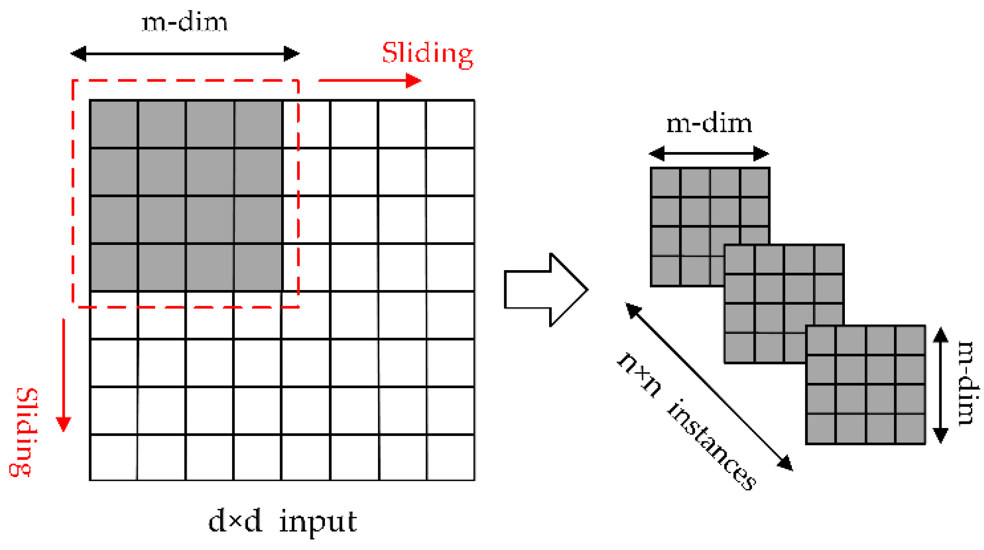
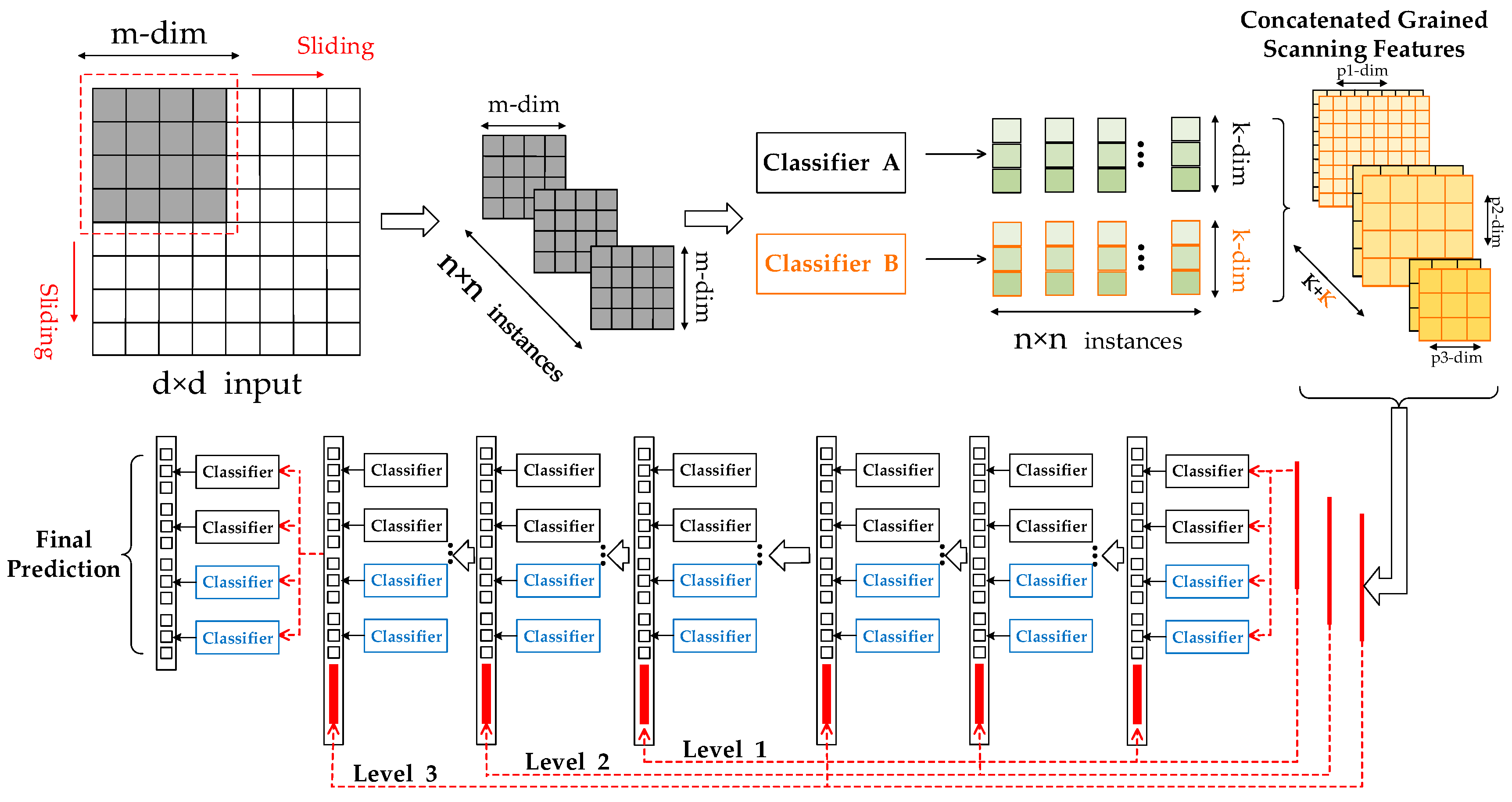
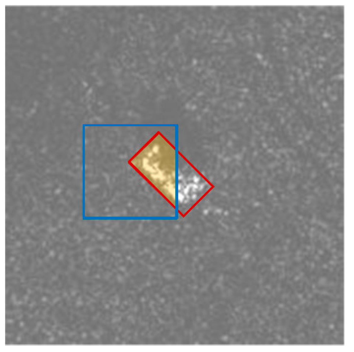
Figure 1.
The process of extracting the original image features by sliding the pane.
Figure 1.
The process of extracting the original image features by sliding the pane.
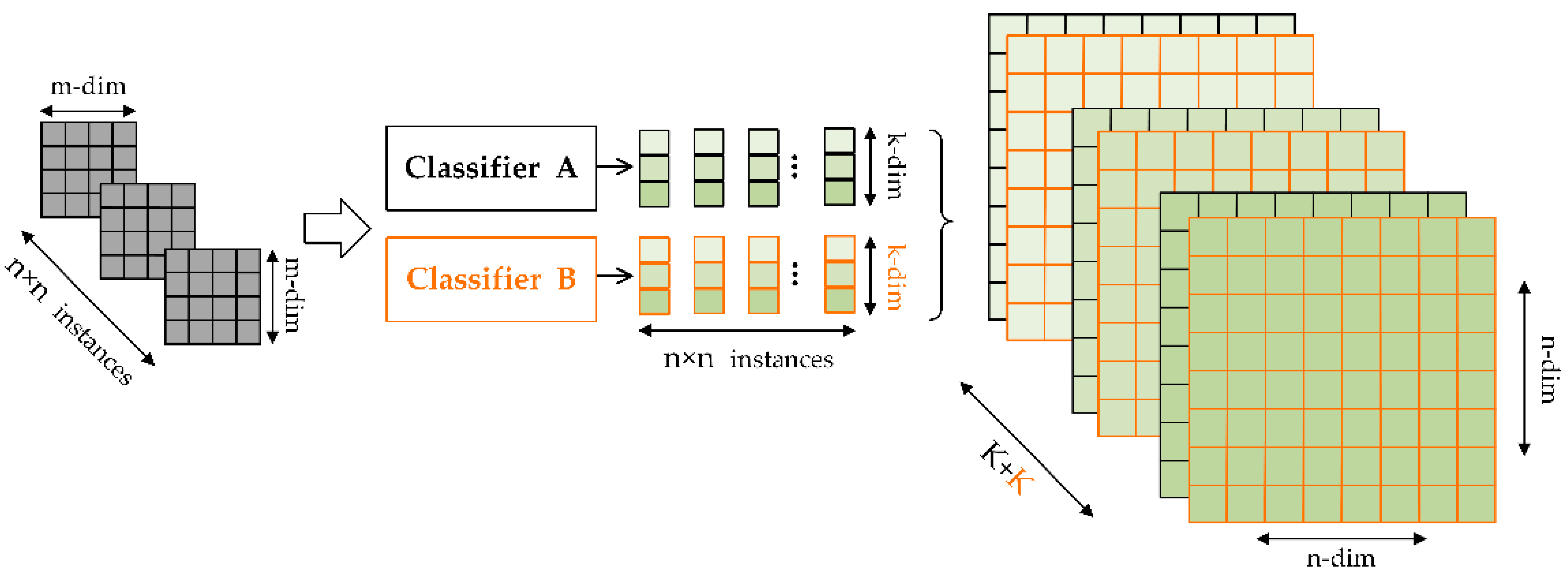
Figure 2.
The formation and transformation of second-stage features vectors.
Figure 2.
The formation and transformation of second-stage features vectors.
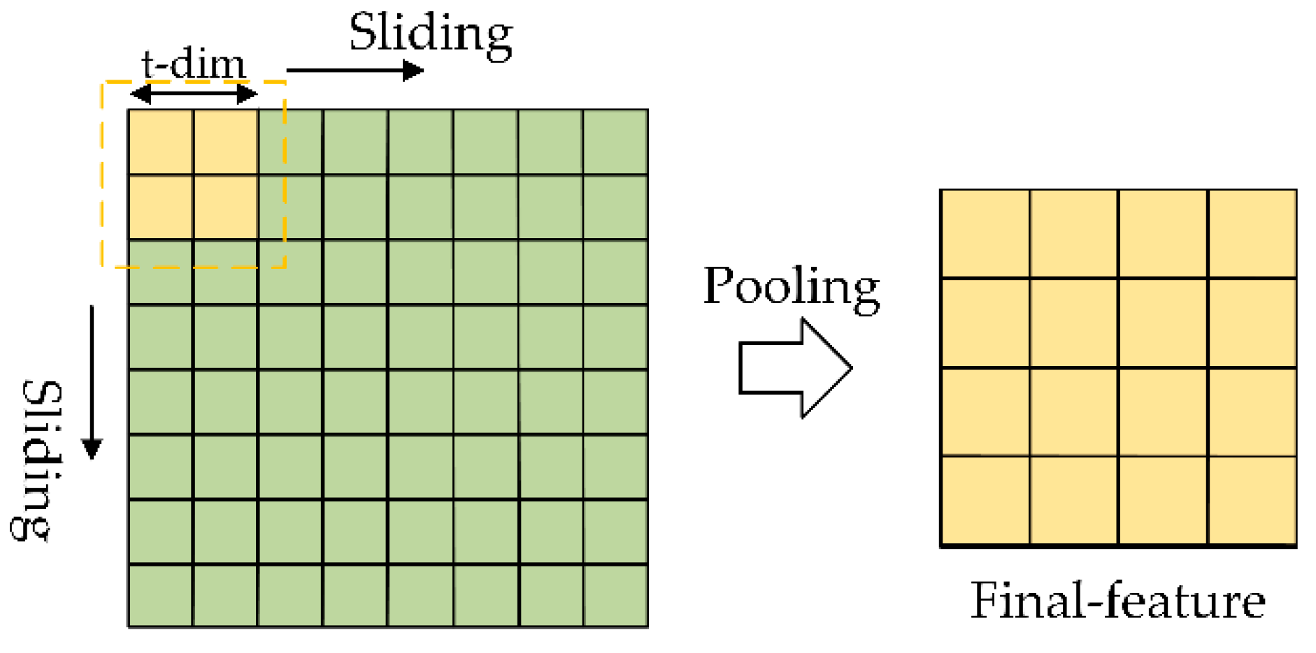
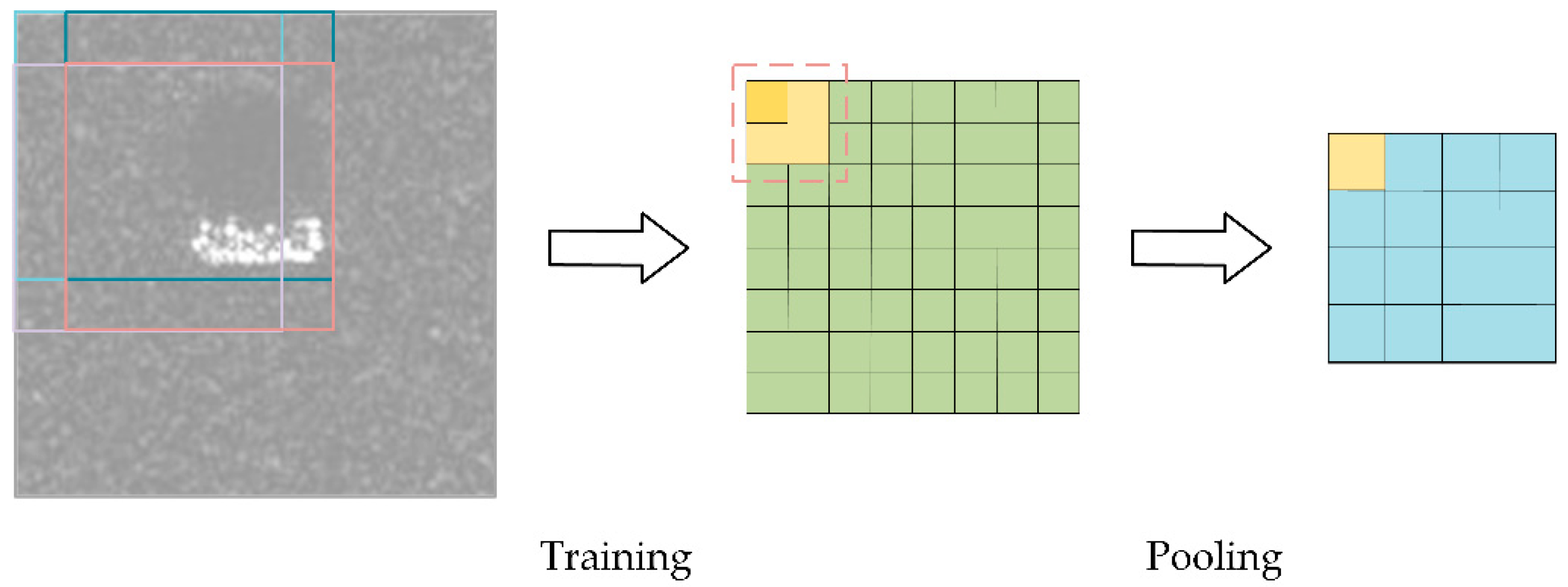
Figure 3.
Pooling to obtain final feature vectors.
Figure 3.
Pooling to obtain final feature vectors.
Figure 4.
Process of the cascade.
Figure 4.
Process of the cascade.
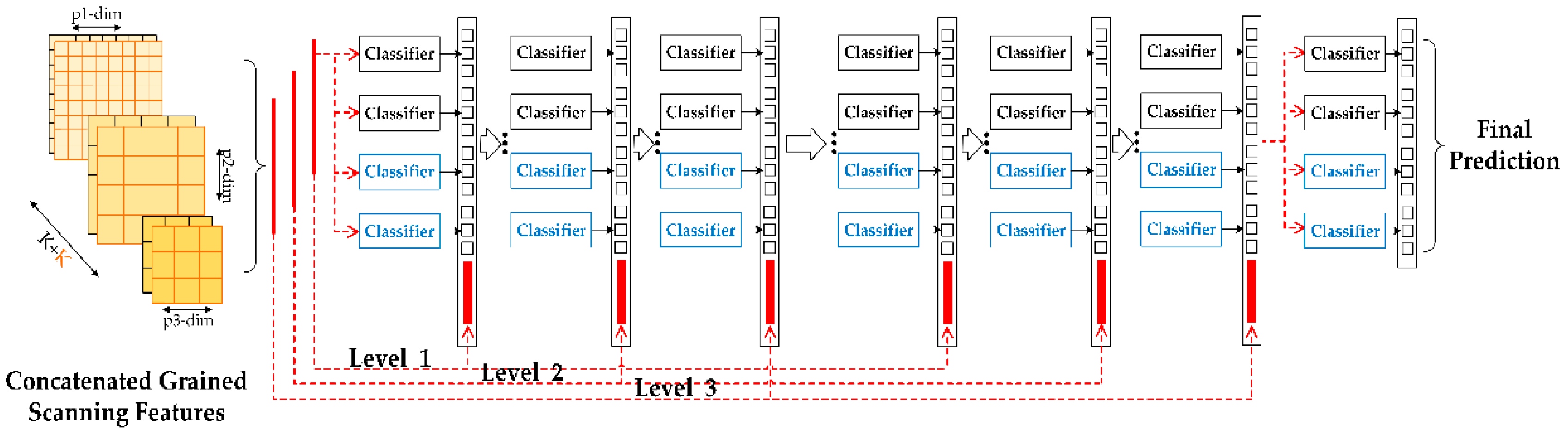
Figure 5.
The overall structure of the multi-grained cascade forest (gcForest).
Figure 5.
The overall structure of the multi-grained cascade forest (gcForest).
Figure 6.
Feature evolution.
Figure 6.
Feature evolution.
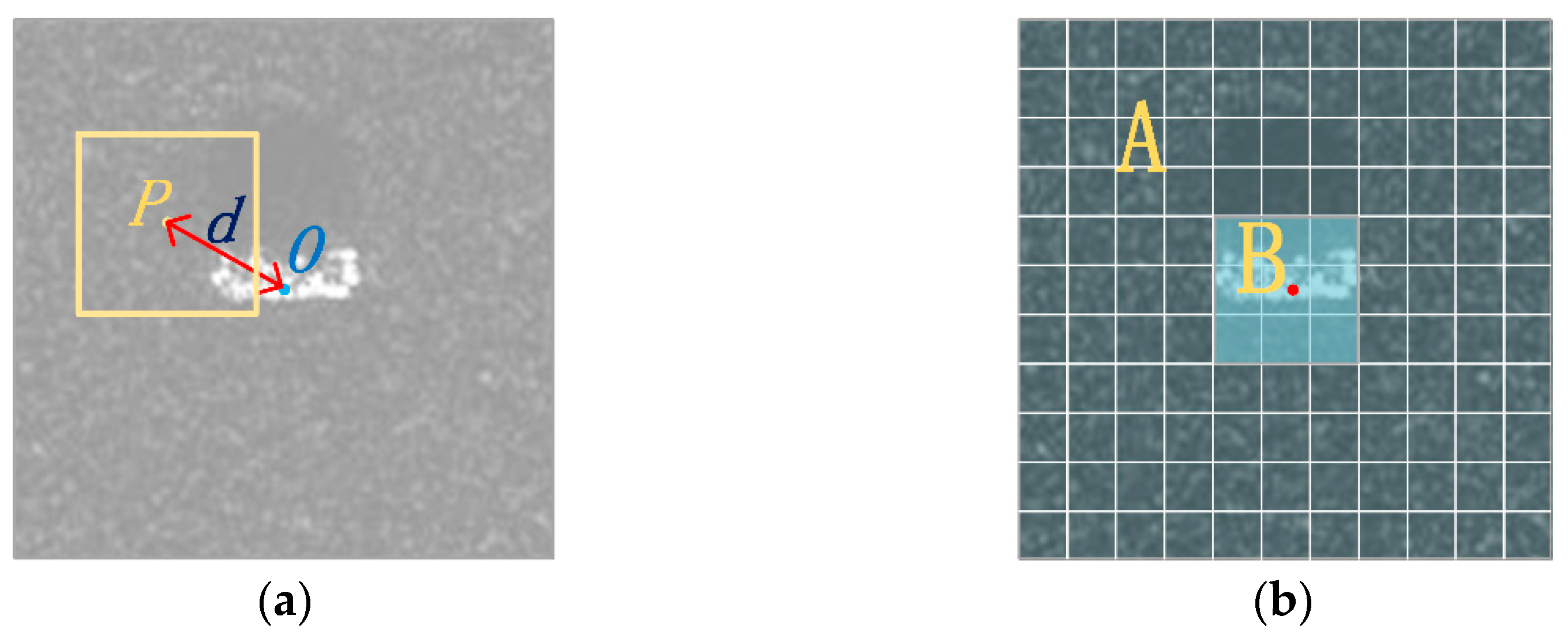
Figure 7.
Description of Euclidean distance pooling. (a) The distance between the center of the image and the center of the pane; (b) the weight range partition diagram.
Figure 7.
Description of Euclidean distance pooling. (a) The distance between the center of the image and the center of the pane; (b) the weight range partition diagram.
Figure 8.
Description of overlap degree weighted pooling.
Figure 8.
Description of overlap degree weighted pooling.
Figure 9.
Ten classes of ground military targets’ optical and synthetic aperture radar (SAR) images.
Figure 9.
Ten classes of ground military targets’ optical and synthetic aperture radar (SAR) images.
Figure 10.
The training time of estimators with different size.
Figure 10.
The training time of estimators with different size.
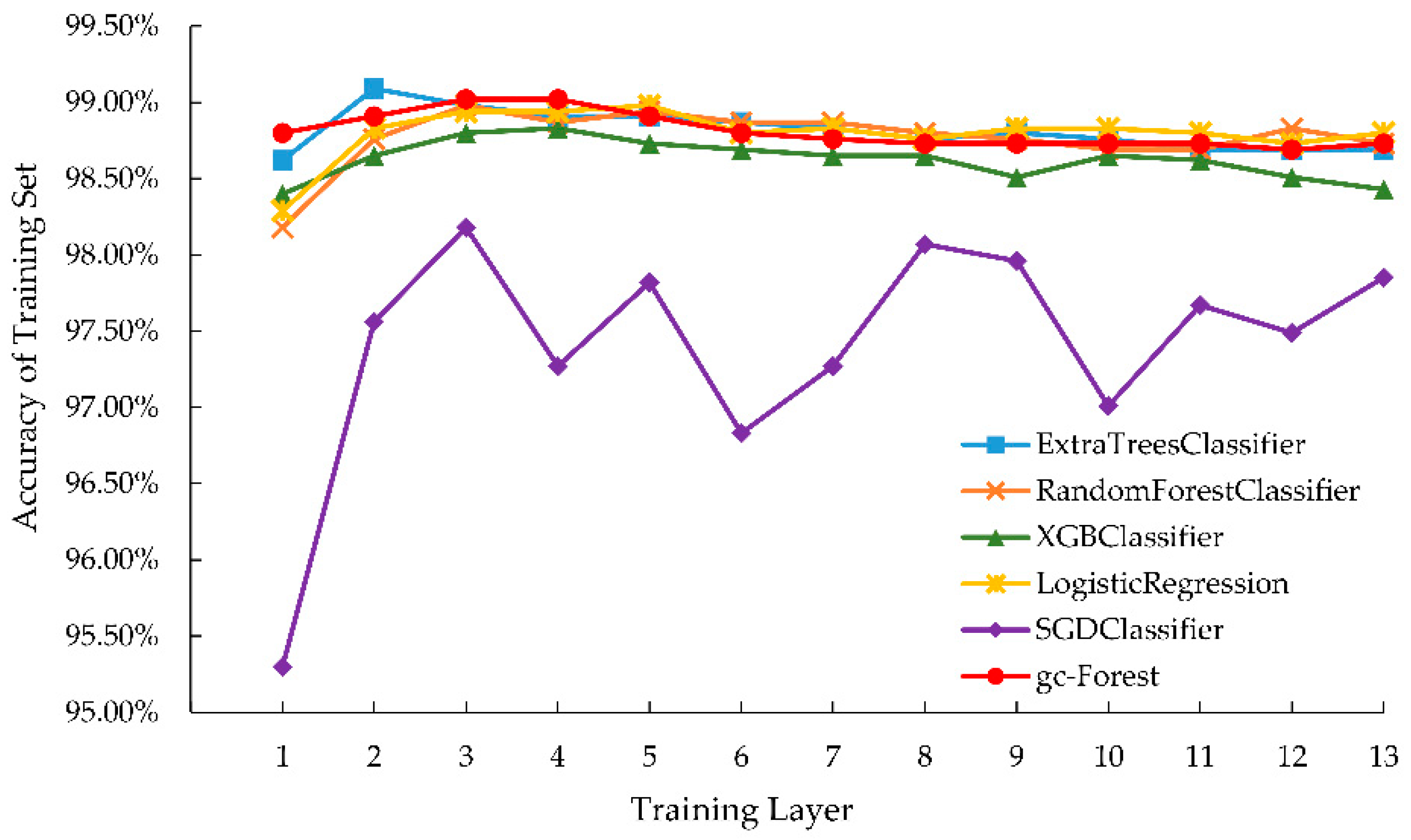
Figure 11.
Training set classification accuracy of gcForest and its built-in classifiers in each layer.
Figure 11.
Training set classification accuracy of gcForest and its built-in classifiers in each layer.
Figure 12.
Test set classification accuracy of gcForest and its built-in classifiers in each layer.
Figure 12.
Test set classification accuracy of gcForest and its built-in classifiers in each layer.
Figure 13.
Test set classification accuracy of RandomForestClassifier with different sizes.
Figure 13.
Test set classification accuracy of RandomForestClassifier with different sizes.
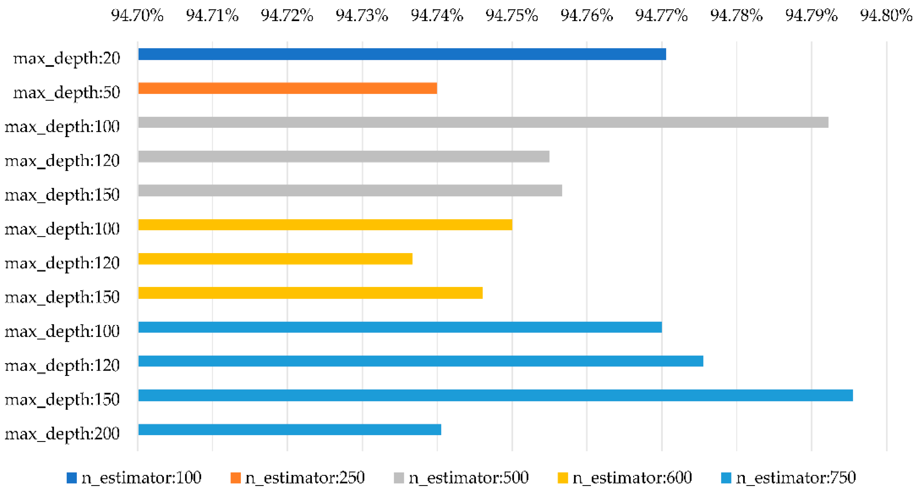
Figure 14.
Test set classification accuracy of ExtraTreesClassifier with different sizes.
Figure 14.
Test set classification accuracy of ExtraTreesClassifier with different sizes.
Figure 15.
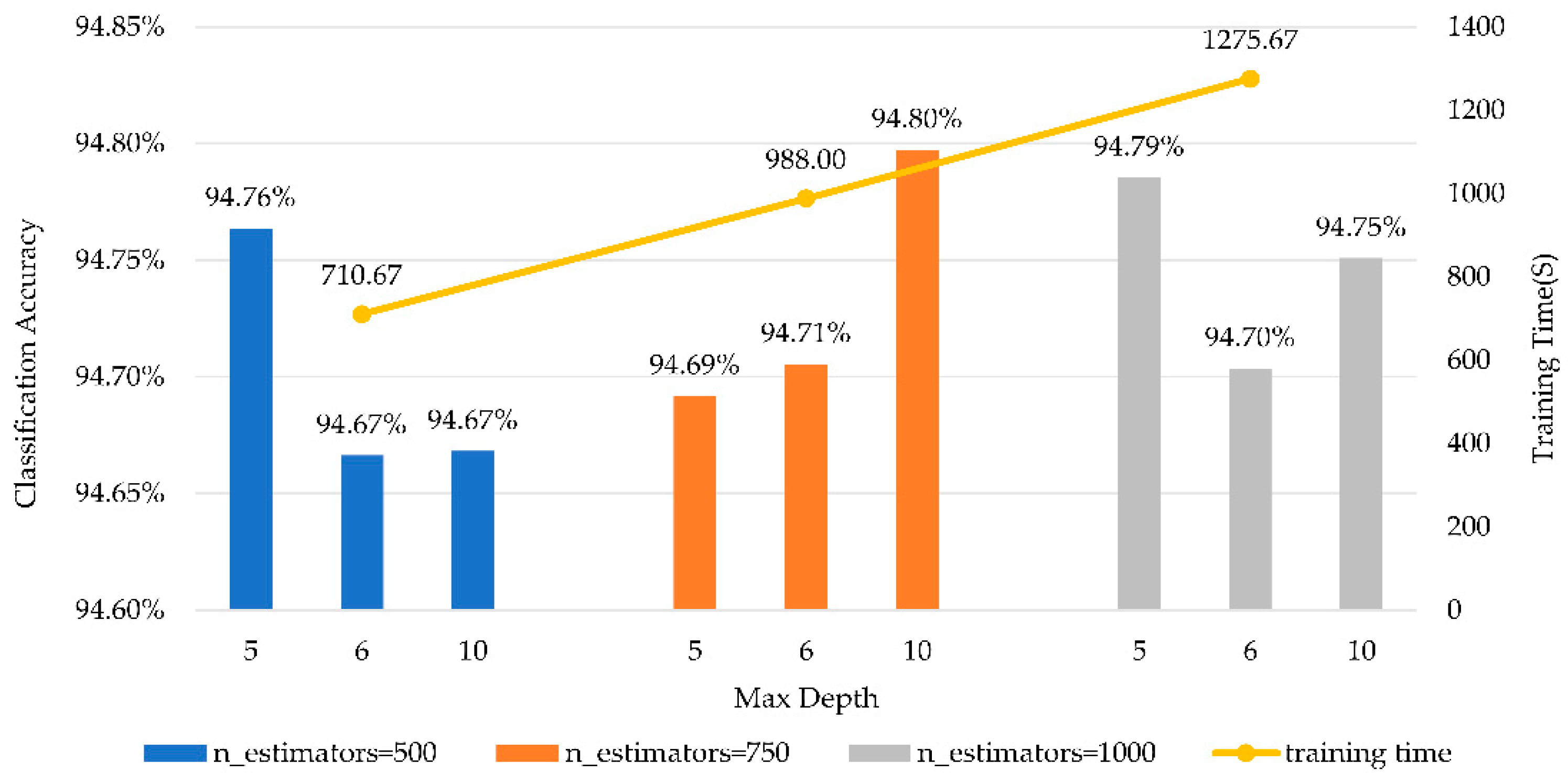
Accuracy and time cost for the test set using XGBClassifier with different sizes.
Figure 15.
Accuracy and time cost for the test set using XGBClassifier with different sizes.
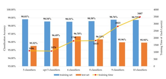
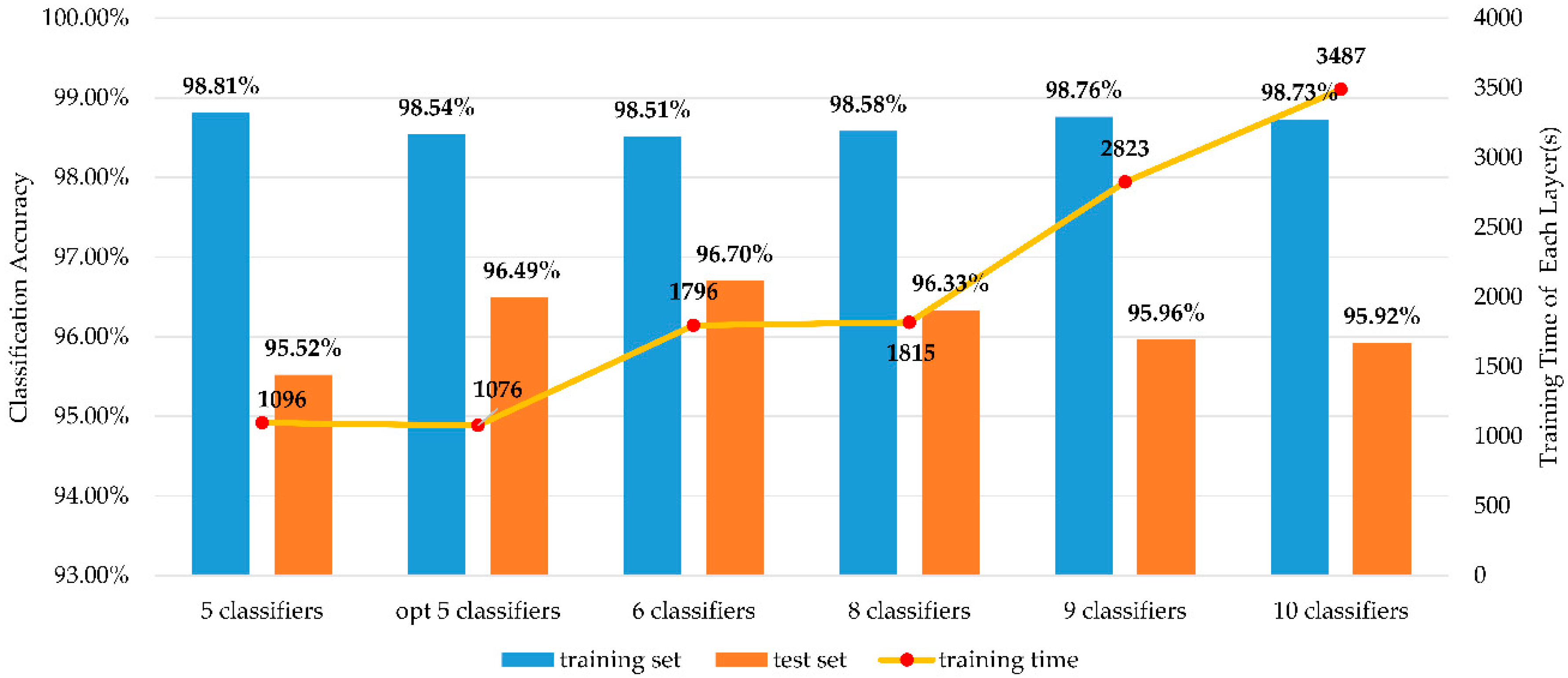
Figure 16.
The accuracy and per layer training time of different combinations.
Figure 16.
The accuracy and per layer training time of different combinations.
Table 1.
Weights for different distance panes.
Table 1.
Weights for different distance panes.
| d | Update Weights |
|---|
| |
| |
Table 2.
Ten classes of moving and stationary target acquisition and recognition (MSTAR) targets and their sample numbers.
Table 2.
Ten classes of moving and stationary target acquisition and recognition (MSTAR) targets and their sample numbers.
| | Training Set | Test Set |
|---|
| 2S1 | 299 | 274 |
| BMP2 | 233 | 195 |
| BRDM2 | 298 | 274 |
| BTR60 | 256 | 195 |
| BTR70 | 233 | 196 |
| D7 | 299 | 274 |
| T62 | 298 | 273 |
| T72 | 232 | 196 |
| ZIL131 | 299 | 274 |
| ZSU234 | 299 | 274 |
| Total | 2746 | 2425 |
Table 3.
Confusion matrix of the MSTAR dataset using gcForest.
Table 3.
Confusion matrix of the MSTAR dataset using gcForest.
| | 2S1 | BMP2 | BRDM2 | BTR60 | BTR70 | D7 | T62 | T72 | ZIL131 | ZSU234 | Recall |
|---|
| 2S1 | 261 | 3 | 3 | 4 | 0 | 1 | 1 | 0 | 0 | 1 | 95.26% |
| BMP2 | 0 | 170 | 2 | 9 | 2 | 0 | 0 | 12 | 0 | 0 | 87.18% |
| BRDM2 | 0 | 0 | 268 | 0 | 0 | 0 | 0 | 0 | 1 | 5 | 97.81% |
| BTR60 | 0 | 1 | 4 | 173 | 4 | 0 | 0 | 2 | 11 | 0 | 88.72% |
| BTR70 | 0 | 0 | 0 | 1 | 193 | 0 | 0 | 2 | 0 | 0 | 98.47% |
| D7 | 0 | 0 | 0 | 0 | 0 | 271 | 0 | 0 | 3 | 0 | 98.90% |
| T62 | 0 | 0 | 0 | 0 | 0 | 0 | 271 | 0 | 1 | 1 | 99.27% |
| T72 | 0 | 1 | 2 | 0 | 0 | 0 | 0 | 193 | 0 | 0 | 98.47% |
| ZIL131 | 0 | 0 | 0 | 0 | 0 | 1 | 0 | 0 | 272 | 1 | 99.27% |
| ZSU234 | 0 | 0 | 0 | 0 | 0 | 1 | 0 | 0 | 0 | 273 | 99.63% |
| Avg. | 96.70% |
Table 4.
Detailed comparison of the classification performance under different methods.
Table 4.
Detailed comparison of the classification performance under different methods.
| | 2S1 | BMP2 | BRDM2 | BTR60 | BTR70 | D7 | T62 | T72 | ZIL131 | ZSU234 | Avg. |
|---|
| OptimizedgcForest | 95.26% | 87.18% | 97.81% | 88.72% | 98.47% | 98.90% | 99.27% | 98.47% | 99.27% | 99.64% | 96.70% |
| Distance gcForest | 94.16% | 85.64% | 97.81% | 90.77% | 98.47% | 99.64% | 99.27% | 98.98% | 99.27% | 99.64% | 96.74% |
| Overlap gcForest | 94.53% | 88.21% | 97.45% | 91.28% | 97.96% | 98.91% | 98.90% | 98.47% | 99.27% | 99.64% | 96.78% |
| Initial gcForest | 56.57% | 80.00% | 71.17% | 84.10% | 90.31% | 87.23% | 63.74% | 90.31% | 99.64% | 99.64% | 81.77% |
| MSCAE | 97.44% | 85.64% | 94.16% | 99.48% | 97.44% | 98.91% | 99.49% | 92.67% | 99.27% | 99.64% | 96.54% |
| ED-AE | 93.80% | 87.90% | 96.72% | 91.79% | 92.86% | 98.91% | 94.14% | 79.55% | 94.53% | 99.64% | 91.29% |
| NMF | 100% | 91.01% | 97.91% | 94.87% | 97.87% | 98.32% | 96.38% | 94.70% | 97.27% | 95.54% | 94.20% |
| MSR | 88.1% | 76.02% | 78.2% | 97.8% | 97.1% | 99.3% | 96.9% | 99.3% | 97.4% | 99.6% | 92.79% |
| Riemannian Manifolds | 88.3% | 96.9% | 82.1% | 98.5% | 96.7% | 99.3% | 99.6% | 97.8% | 99.6% | 99.6% | 94.88% |
Table 5.
Initial experimental parameter setting.
Table 5.
Initial experimental parameter setting.
| gcForest Models | Parameter Setting |
|---|
| Multi-Grained Scanning | Number of Classifiers | 2 |
| Types of Classifiers | ExtraTreesClassifier |
| RandomForestClassifier |
| Condition to Stop Growing Trees | Tree depth reaches 500 |
| Size of Sliding Panes | 12, 24, 48 |
| Cascade | Number of Classifiers | 8 |
| Types of Classifiers | XGBClassifier |
| RandomForestClassifier |
| ExtraTreesClassifier |
| LogisticRegression |
| Condition to Stop Growing Trees | Tree depth reaches 500 |
Table 6.
Effects of different sliding panes sizes on accuracy and training time.
Table 6.
Effects of different sliding panes sizes on accuracy and training time.
| | 12 * 12 | 24 * 24 | 36 * 36 | 48 * 48 | 60 * 60 | 72 * 72 | 84 * 84 | 90 * 90 | 96 * 96 |
|---|
| Training Set | 57.74% | 69.92% | 78.08% | 83.72% | 84.71% | 86.72% | 89.15% | 90.05% | 89.15% |
| Test Set | 29.44% | 36.54% | 45.24% | 57.86% | 63.55% | 68.82% | 76.54% | 80.54% | 79.55% |
| Training Time (s) | 97,024 | 89,666 | 63,686 | 55,896 | 40,255 | 11,122 | 1504 | 399 | 19 |
Table 7.
Original experimental parameter setting of multi-grained scanning.
Table 7.
Original experimental parameter setting of multi-grained scanning.
| Classifier Types | Parameter Setting |
|---|
| RandomForestClassifier | Criterion = ‘gini’, max_features = sqrt(n_features), n_estimators = 500, max_depth = 100, min_samples_leaf = 10 |
| ExtraTreesClassifier | Criterion = ‘gini’, max_features = sqrt(n_features), n_estimators = 500, max_depth = 100, min_samples_leaf = 10 |
| LogisticRegression | Penalty = ‘l2’, tol = 0.0001 |
Table 8.
Accuracy using different classifiers.
Table 8.
Accuracy using different classifiers.
| Classifier Types | Training Set | Test Set |
|---|
| RandomForestClassifier | 88.64% | 72.70% |
| ExtraTreesClassifier | 87.98% | 76.62% |
| LogisticRegression | 86.13% | 85.65% |
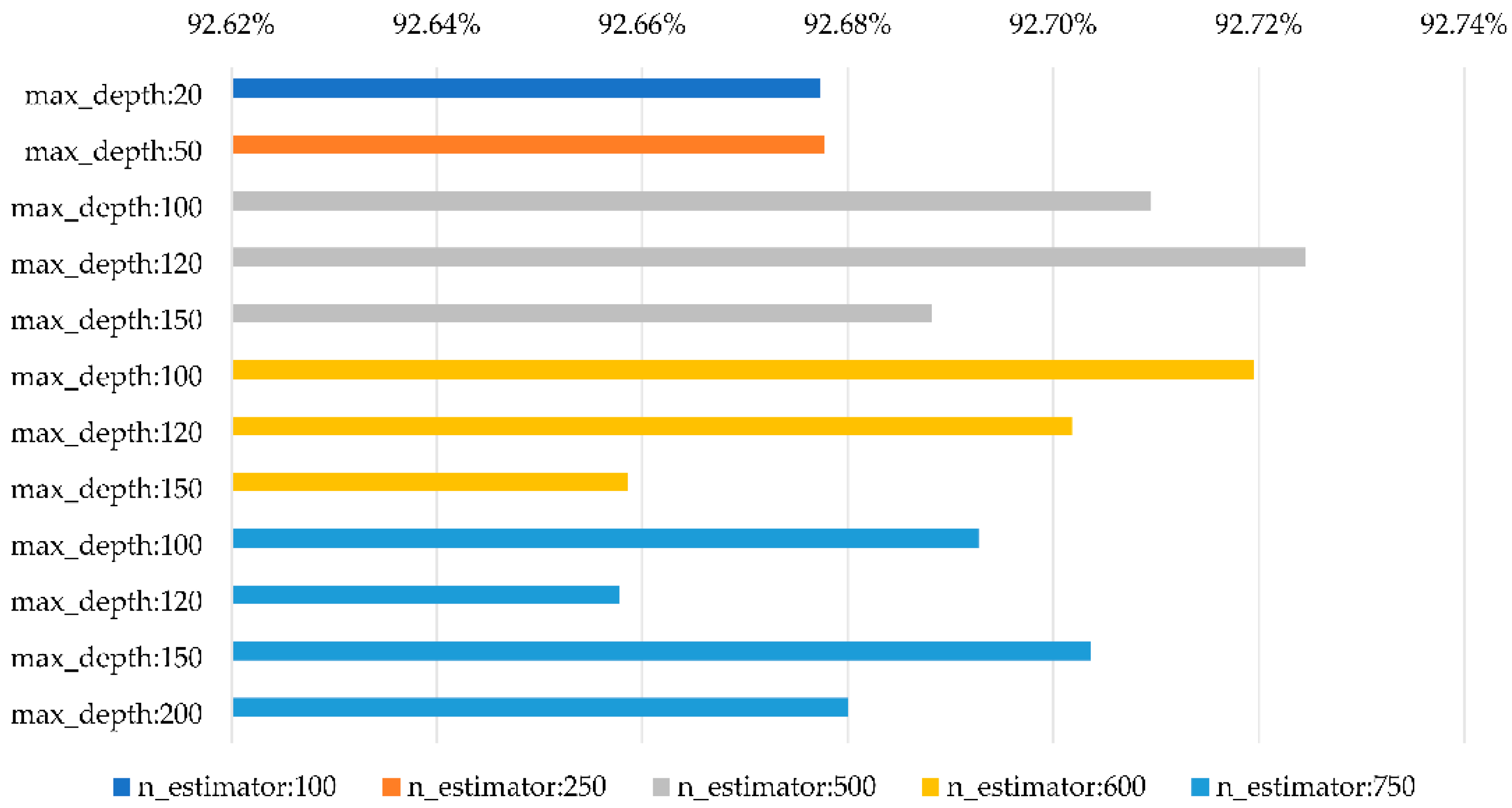
Table 9.
Accuracy of RandomForestClassifier and ExtraTreesClassifier with different sizes.
Table 9.
Accuracy of RandomForestClassifier and ExtraTreesClassifier with different sizes.
| Parameter Setting | RandomForestClassifier | ExtraTreesClassifier |
|---|
| Training Set | Test Set | Training Set | Test Set |
|---|
| n_estimators = 100, max_depth = 20 | 88.20% | 72.49% | 88.60% | 76.21% |
| n_estimators = 250, max_depth = 50 | 87.91% | 72.78% | 89.29% | 76.26% |
| n_estimators = 500, max_depth = 100 | 88.93% | 72.91% | 89.15% | 76.54% |
| n_estimators = 600, max_depth = 120 | 88.35% | 72.78% | 87.87% | 76.78% |
| n_estimators = 750, max_depth = 150 | 89.15% | 72.82% | 88.75% | 76.41% |
Table 10.
Final configuration of multi-grained scanning.
Table 10.
Final configuration of multi-grained scanning.
| Classifier Types | Parameter Setting | Pane Size |
|---|
| ExtraTreesClassifier | Criterion = ‘gini’, max_features = sqrt(n_features), n_estimators = 600, max_depth = 120 | 72, 84, 90, 96 |
| RandomForestClassifier | Criterion = ‘gini’, max_features = sqrt(n_features), n_estimators = 500, max_depth = 100 | 72, 84, 90, 96 |
| LogisticRegression | Penalty = ‘l2’, tol = 0.0001 | 84, 90 |
Table 11.
Initial experimental parameter setting of the cascade forest.
Table 11.
Initial experimental parameter setting of the cascade forest.
| Classifier Types | Parameter Setting |
|---|
| ExtraTreesClassifier | Criterion = ‘gini’, max_features = sqrt(n_features), n_estimators = 500, max_depth = 100 |
| RandomForestClassifier | Criterion = ‘gini’, max_features = sqrt(n_features), n_estimators = 500, max_depth = 100 |
| XGBClassifier | base_score = 0.5, booster = ‘gbtree’, max_depth = 5, learning_rate = 0.1, n_estimators = 500, objective = ‘multi: softprob’ |
| LogisticRegression | Penalty = ‘l2’, tol = 0.0001 |
| SGDClassifier | Penalty = ‘l2’, loss = ‘modified_huber’ |
Table 12.
Mean classification accuracy of gcForest and built-in classifiers.
Table 12.
Mean classification accuracy of gcForest and built-in classifiers.
| Classifier Types | Training Set | Test Set |
|---|
| ExtraTreesClassifier | 98.82% | 94.88% |
| RandomForestClassifier | 98.77% | 94.60% |
| XGBClassifier | 98.62% | 95.20% |
| LogisticRegression | 98.80% | 95.52% |
| SGDClassifier | 97.41% | 95.96% |
| gcForest | 98.81% | 95.52% |
Table 13.
The average training precision of different loss functions of the SGDClassifier.
Table 13.
The average training precision of different loss functions of the SGDClassifier.
| Parameter Setting | Training Set | Test Set |
|---|
| loss = ‘modified_hube’ | 95.43% | 95.23% |
| loss = ‘log’ | 97.42% | 95.37% |
Table 14.
Selection of the number and combination of different classifiers.
Table 14.
Selection of the number and combination of different classifiers.
| Classifier Type | Classifier Number |
|---|
| 5 | 6 | 8 | 9 | 10 |
|---|
| ExtraTreesClassifier | 1 | 1 | 1 | 1 | 1 |
| RandomForestClassifier | 1 | 1 | 1 | 1 | 1 |
| XGBClassifier (max_depth = 10, n_estimators = 750) | 1 | 1 | 1 | 2 | 2 |
| XGBClassifier (max_depth = 5, n_estimators = 500) | 0 | 1 | 1 | 1 | 2 |
| LogisticRegression | 1 | 1 | 2 | 2 | 2 |
| SGDClassifier | 1 | 1 | 2 | 2 | 2 |
Table 15.
Optimized classifier selection and its parameter settings.
Table 15.
Optimized classifier selection and its parameter settings.
| Classifier Type | Parameter Setting |
|---|
| ExtraTreesClassifier | Criterion = ‘gini’, max_features = sqrt(n_features), n_estimators = 500, max_depth = 100 |
| RandomForestClassifier | Criterion = ‘gini’, max_features = sqrt(n_features), n_estimators = 600, max_depth = 100 |
| XGBClassifier | base_score = 0.5, booster = ‘gbtree’, max_depth = 10, learning_rate = 0.1, n_estimators = 750, objective = ‘multi: softprob’ |
| XGBClassifier | base_score = 0.5, booster = ‘gbtree’, max_depth = 5, learning_rate = 0.1, n_estimators = 500, objective = ‘multi: softprob’ |
| LogisticRegression | Penalty = ‘l2’, tol = 0.0001 |
| SGDClassifier | Penalty = ‘l2’, loss = ‘log’ |
Table 16.
Optimized experimental parameter setting.
Table 16.
Optimized experimental parameter setting.
| gcForest Models | Parameter Setting |
|---|
| Multi-Grained Scanning | Number of Classifiers | 3 |
| Size of Sliding Panes | 72, 84, 90, 96 |
| Types of Classifiers | ExtraTreesClassifier | Criterion = ‘gini’, max_features = sqrt(n_features), n_estimators = 600, max_depth = 120 |
| RandomForestClassifier | Criterion = ‘gini’, max_features = sqrt(n_features), n_estimators = 500, max_depth = 100 |
| LogisticRegression | Penalty = ‘l2’, tol = 0.0001 |
| Cascade | Number of Classifiers | 6 |
| Types of Classifiers | ExtraTreesClassifier | Criterion = ‘gini’, max_features = sqrt(n_features), n_estimators = 500, max_depth = 100 |
| RandomForestClassifier | Criterion = ‘gini’, max_features = sqrt(n_features), n_estimators = 600, max_depth = 100 |
| XGBClassifier | base_score = 0.5, booster = ‘gbtree’, max_depth = 10, learning_rate = 0.1, n_estimators = 750, objective = ‘multi: softprob’ |
| XGBClassifier | base_score = 0.5, booster = ‘gbtree’, max_depth = 5, learning_rate = 0.1, n_estimators = 500, objective = ‘multi: softprob’ |
| LogisticRegression | penalty = ‘l2’, tol = 0.0001 |
| SGDClassifier | penalty = ‘l2’, loss = ‘log’ |
Table 17.
Time consumption of each stage and each layer.
Table 17.
Time consumption of each stage and each layer.
| Cost Time (s) | Initial | Optimized | Distance | Overlap |
|---|
| Multi-Grained Scanning (Total) | 567,868 | 67,169 | 67,169 | 67,169 |
| Cascade (Total) | 126,179 | 37,954 | 56,975 | 56,323 |
| Cascade (Each layer) | 9801 | 1796 | 1859 | 1922 |
| gcForest (Total) | 694,047 | 105,123 | 124,144 | 123,492 |


