Predicting Forage Quality of Grasslands Using UAV-Borne Imaging Spectroscopy

Abstract

The timely knowledge of forage quality of grasslands is vital for matching the demands in animal feeding. Remote sensing (RS) is a promising tool for estimating field-scale forage quality compared with traditional methods, which usually do not provide equally detailed information. However, the applicability of RS prediction models depends on the variability of the underlying calibration data, which can be brought about by the inclusion of a multitude of grassland types and management practices in the model development. Major aims of this study were (i) to build forage quality estimation models for multiple grassland types based on an unmanned aerial vehicle (UAV)-borne imaging spectroscopy and (ii) to generate forage quality distribution maps using the best models obtained. The study examined data from eight grasslands in northern Hesse, Germany, which largely differed in terms of vegetation type and cutting regime. The UAV with a hyperspectral camera on board was utilised to acquire spectral images from the grasslands, and crude protein (CP) and acid detergent fibre (ADF) concentration of the forage was assessed at each cut. Five predictive modelling regression algorithms were applied to develop quality estimation models. Further, grassland forage quality distribution maps were created using the best models developed. The normalised spectral reflectance data showed the strongest relationship with both CP and ADF concentration. From all predictive algorithms, support vector regression provided the highest precision and accuracy for CP estimation (median normalised root mean square error prediction (nRMSE_p) = 10.6%), while cubist regression model proved best for ADF estimation (median nRMSE_p = 13.4%). The maps generated for both CP and ADF showed a distinct spatial variation in forage quality values for the different grasslands and cutting regimes. Overall, the results disclose that UAV-borne imaging spectroscopy, in combination with predictive modelling, provides a promising tool for accurate forage quality estimation of multiple grasslands.

1. Introduction

In Europe, approximately 30% to 35% of the agricultural area consists of grasslands [1]. Mainly permanent grasslands are incredibly variable in species composition, biodiversity, and management practices, as well as in productivity [2]. Food provisions as forage for ruminants and herbivores and as biomass substrate for energy production are the most comprehensive ecosystem services from grasslands. There exists a multitude of destructive and non-destructive methods to measure or estimate the production and quality of the forage [3,4,5]. Timely and accurate information about forage quality is essential to match available feed on offer with animals’ demand.

Usually, farmers use visual criteria to evaluate forage quality, such as the plants’ phenological stage, leafiness, or colour. Additionally, lab-based chemical analysis and near-infrared reflectance spectroscopy (NIRS) are utilised by agronomists to evaluate forage quality [6]. Lab-based methods are used to determine chemical forage components that relate to the digestibility of the forage. Acid detergent fibre (ADF), which represents cellulose, lignin, and silica, is an important parameter that is negatively correlated with forage digestibility [6,7]. The protein concentration of forages is another parameter essential for the creation of adequate fodder rations. Protein consists mainly of amino acids, which are fundamental elements of all cells and tissues. Protein is an essential component of ruminant nutrition and provides nitrogen for ruminants’ metabolism and production of milk and meat [8].

Remote sensing (RS) is a non-destructive method for estimating grassland biomass and forage quality [9,10,11]. From satellite RS to field spectroscopy and from optical RS to synthetic aperture radar were employed for forage quality monitoring and mapping [5,12]. A literature review on RS based forage quality estimation studies published between 2004 and 2018 shows that more than 60% of studies (21 out of a total of 31 reviewed studies) have utilised field spectroscopy. Often, point-level spectral reflectance data from visible to short-wave infrared regions of the electromagnetic spectrum are collected in field spectroscopy [13]. Crude protein (CP), nitrogen (N), neutral detergent fibre (NDF), and ADF are the most common forage quality parameters that have been estimated using field spectroscopy data for different grasslands with significant accuracy [14,15,16,17,18].

Point-level data observation is laborious and challenging to collect over large areas. The application of imaging spectroscopy (also known as hyperspectral imaging) mounted on higher-altitude platforms (i.e., airborne, space-borne) could overcome these disadvantages. Imaging spectroscopy is the “acquisition of images in many (hundreds) narrow contiguous spectral bands” [19]. Instead of point observation, imaging spectroscopy provides a two-dimensional image with each pixel containing spectral reflectance data. Airborne imaging spectroscopy has been utilised for forage quality mapping in grassland [16,20,21], but conducting manned airborne mission requires extensive well-ahead planning. On the contrary, an unmanned aerial vehicle (UAV) allows the collection of low altitude images over large areas with less effort and relatively low costs.

UAV as an RS platform for both multi- and hyperspectral imaging has been frequently applied for field-scale vegetation mapping in the last few years owing to miniature sensor availability and the advancement of computer vision techniques. Concerning grassland monitoring and mapping, the UAV-borne RS has been employed mainly for grassland biomass estimation with multispectral imaging [22], imaging spectroscopy [23,24], and consumer-grade cameras [25,26]. Only two studies that utilised UAV-borne imaging spectroscopy data for forage quality estimation are known to the authors [23,24], and the results showed that UAV-borne imaging spectroscopy data could accurately predict forage quality parameters. However, those studies have only focused on experimental plots, and no study has evaluated the UAV-borne imaging spectroscopy for forage quality estimation under practical field conditions including different grassland types in terms of plant community composition and with a wide range of management practices.

Except for the spectral data collection method, the model development for forage quality estimation employed various techniques. In general, forage quality modelling utilised actual reflectance data or transformed spectral reflectance data, among which normalised spectra, derivative spectra, and continuum removal spectra. The most frequently applied statistical modelling method is the linear regression (simple linear, step-wise linear) with selected highly correlated spectral features, such as wavebands [20,27], normalised difference spectral indices (NDSIs) [18,24,28], spectral ratios (SRs) [15,29], and other well-known vegetation indices (e.g., NDVI, SAVI, NDRE) [17,23]. Predictive modelling (also known as machine learning) algorithms, such as partial least squares regression (PLSR) [16,27,30,31,32], random forest regression (RFR) [24,33,34], and artificial neural network [20,21,35], were employed to estimate forage quality parameters using highly correlated spectral reflectance data. Predictive modelling algorithms frequently enhanced the predictive capability compared with the simpler linear regression models [24,34]. Moreover, there are several other algorithms in predictive modelling, namely, Gaussian processing regression (GPR), support vector regression (SVR), and cubist regression (CBR), that have not been examined with spectral data to estimate forage quality.

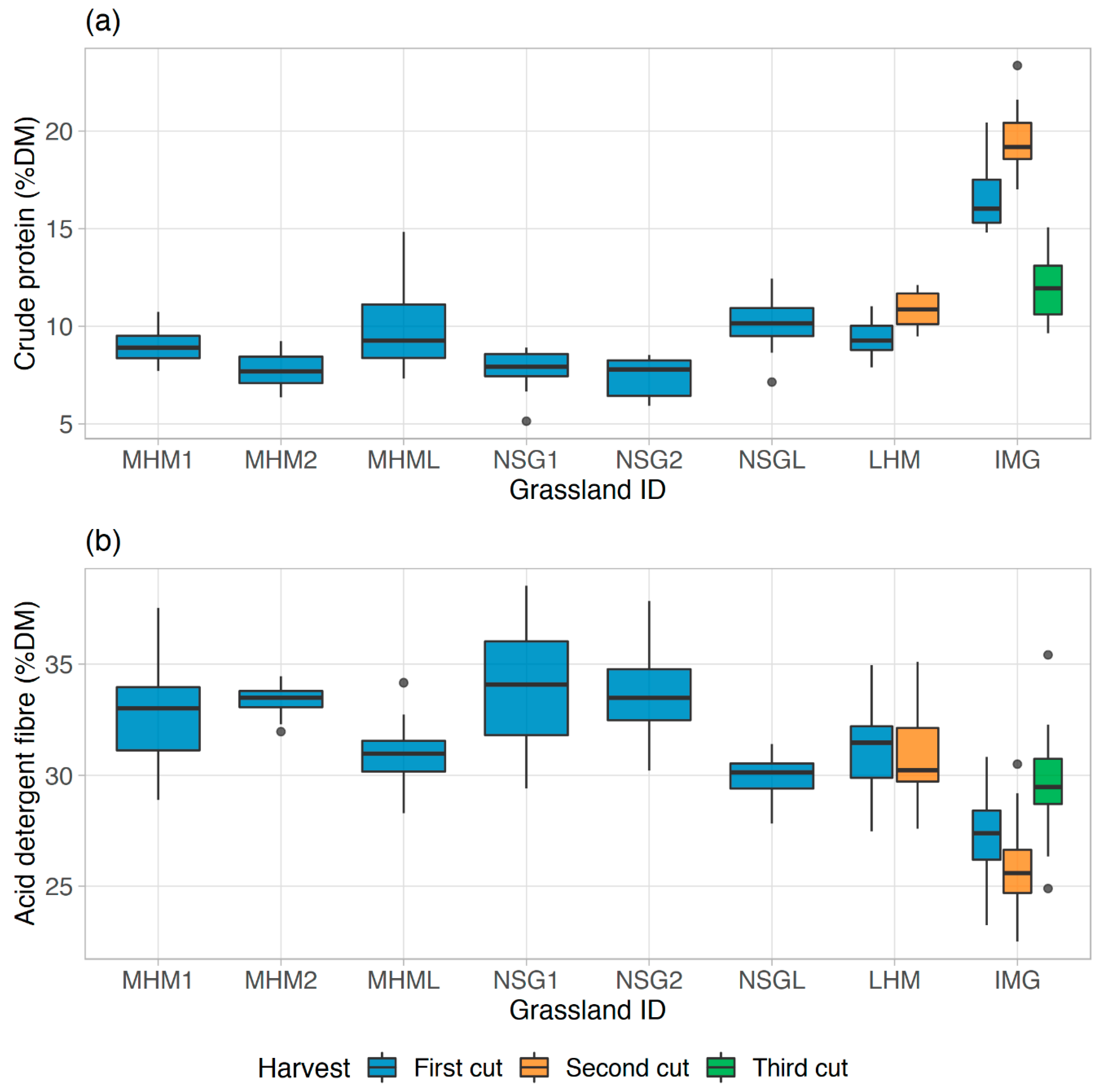
Typically, the models developed to estimate forage quality using spectral data are restricted to single grassland types. Consequently, the transferability of the models to other grassland types is limited due to the low variability of the underlying training data. Therefore, a general model that can estimate forage quality parameters, irrespective of the grassland type, would be a preferable solution. Thus, we hypothesise that the usage of spectral data over different grasslands with predictive modelling algorithms can build models to estimate major forage quality parameters regardless of the grassland type or management practice. The overall objective of this study is to develop comprehensive predictive models to estimate CP and ADF concentrations (from now on referred to as CP and ADF) on the field level, using UAV-borne imaging spectroscopy data from different grasslands. Specifically, to build models that can predict values regardless of the grassland type and to examine the effect of grassland type for the model performances. With this in mind, the specific sub-objectives are as follows:

• To understand the relationship between forage quality parameters (CP and ADF) and spectral reflectance;
• To develop models for CP and ADF estimation from imaging spectroscopy data and to evaluate models;
• To create field-level CP and ADF maps for grasslands and describe the spatial and temporal variation of forage quality.

2. Materials and Methods

2.1. Study Area

The study was carried out on eight grasslands with different management practice and species composition.

Table 1. Details of grasslands investigated in the study. (m.a.s.l. = meter above sea level).

Field ID	Vegetation Type	Location (m.a.s.l.)	Short Description
MHM1	Mountain hay meadow	Werra-Meißner district (684)	Nature conservation grassland late harvest, no fertilisation
MHM2	Mountain hay meadow	Biosphere Reserve “Rhön” (739)	Nature conservation grassland late harvest, no fertilisation
NSG1	Nardus stricta grassland	Werra-Meißner district (718)	Nature conservation grassland late harvest, no fertilisation
NSG2	Nardus stricta grassland	Biosphere Reserve “Rhön” (822)	Nature conservation grassland late harvest, no fertilisation
MHML	Former Mountain hay meadow invaded by Lupinus polyphyllus	Biosphere Reserve “Rhön” (839)	Nature conservation grassland late harvest, no fertilisation
NSGL	Former Nardus stricta grassland invaded by Lupinus polyphyllus	Biosphere Reserve “Rhön” (846)	Nature conservation grassland late harvest, no fertilisation
LHM	Lowland hay meadow	Werra-Meißner district (135)	Extensive alluvial grassland, no fertilisation
IMG	Seeded grassland	Werra-Meißner district (199)	Intensive grassland, fertilised

gives details of the grasslands, and Figure 1 shows their locations on the map. Six grasslands were in nature protection areas, where no fertilisation was applied, and they were mowed only once per year. Two of them were mountain hay meadows (MHM), and another two were Nardus stricta grasslands (NSG). MHML and NSGL were MHM and NSG grasslands, which were substantially invaded by the neophyte Lupinus polyphyllus. The lowland hay meadow (LHM) is an extensively utilised grassland located on the Werra riverbank, and it was mowed two times per year. The intensively managed grassland (IMG) was fertilised and was harvested three times per year. All grasslands were in northern Hesse, Germany. MHM1, NSG1, LHM, and IMG grasslands were in Werra-Meißner district in Hesse (EPSG 4326: 9.9° N, 51.3° E) (Figure 1b). The other four grasslands (MHM2, NSG2, MHML, and NSGL) were located in UNSECO Biosphere reserve Rhön (EPSG 4326: 10.0° N, 50.5° E) (Figure 1c).

A 25 m by 50 m rectangle plot (1250 m²) was selected as the study plot in grasslands located in Werra-Meißner district. In each study plot, twenty 1 m² subplots were randomly distributed and selected for destructive biomass samplings. The random sub-plot generation was done in QGIS, with each subplot having a minimum distance of 5 m to the nearest subplot.

The plots in the biosphere reserve Rhön were not allowed to be mown before 15 July and, to replicate different vegetation maturity stages, different sampling design was employed. From the grasslands in biosphere reserve Rhön, a 50 m by 30 m rectangle plot (1500 m²) was chosen as the study plot. A total of fifteen small plots (8 m by 8 m) were established in each study plot, and they were in a regular grid (five rows and three columns). Three 1 m² sampling plots were picked from each small plot as the subplots for destructive biomass sampling.

2.2. Data Collection

2.2.1. The UAV-Borne Imaging Spectroscopy System

The Cubert Hyperspectral Firefleye S185 SE (Cubert GmbH, (Ulm, Germany) www.cubert-gmbh.de) snapshot camera (12 mm focal length) is an imaging spectroscopy sensor that acquires spectral images between 450 and 998 nm. It is a 2D imager with a multi-point spectrometer. The spectral resolution of the sensor (full width at half maximum) is 4.8 nm at 450 nm and 25.6 nm at 850 nm. The camera records a total of 138 spectral bands with a 4 nm sampling interval, but the manufacturer recommended to use only 126 bands between 450 and 950 nm. Each spectral band image is 50 by 50 pixel, and radiometric resolution is 12 bit (0–4096 digital numbers). In addition to the spectral bands, a grayscale panchromatic image is also recorded with 1000 by 990 pixels in size [36,37]. The spatial resolution of the spectral image is 20 cm at 20 m flying height. The captured image from the camera is an image cube that has 126 bands.

The Cubert camera was attached to the UAV (RTK X8 Hyperspectral Mapping, Cubert GmbH, www.cubert-gmbh.de). It is a co-axial multi-rotor UAV equipped with real-time kinematic (RTK) global navigation satellite system (GNSS). It can fly automatically guided with less than 1 m position accuracy. The maximum payload is 2.5 kg, and maximum flight weight is 10 kg. The camera is affixed to a gimble on the UAV, which compensates for pitch and roll movement during the flight, and keeps the camera always nadir looking [38]. Figure 2 shows the UAV and the attached Cubert camera.

2.2.2. Spectral Images and Forage Quality Data

UAV-borne imaging spectroscopy data collection and destructive biomass sampling were carried out on every grassland immediately prior to each cut between May and September in 2018 (

Table 2. Details on samplings of the grasslands investigated in the study.

Field ID	Harvest	Sampling Date	No. of Quality Samples
MHM1	First cut	13 July	20 †
NSG1	First cut	14 July	19 †
MHM2, NSG2, MHML, NSGL	First cut	13 June	20 ‡ (5, 5, 5, 5)
MHM2, NSG2, MHML, NSGL	First cut	27 June	20 ‡ (5, 5, 5, 5)
MHM2, NSG2, MHML, NSGL	First cut	11 July	20 ‡ (5, 5, 5, 5)
LHM	First cut	28 May	20 †
	Second cut	24 September	15 †
IHM	First cut	10 May	20 †
	Second cut	6 June	20 †
	Third cut	1 August	20 †

^† 1 m² plots. ^‡ at each cut, three 1 m² subplots inside the 64 m² plots were sampled, which gives a total of fifteen samples (3 × 5) at each cut for one grassland. However, in the lab analysis, samples from the three sub-plots were mixed and concentration data were determined (five quality samples per cut in one grassland).

).

Spectral images were acquired between 10:00 and 14:00 under clear-sky conditions. Before the UAV flight, four corners of the study area were staked out using the Leica RTK GNSS (Leica Geosystem, www.leica-geosystems.com) and six black-white 1 m² ground control points (GCP) were distributed around the study plot. The coordinates of the GCPs were also measured using the RTK GNSS. The UAV flight mission was done with guided auto-pilot system in parallel flight lines at a flying height of 20 m and a horizontal flying speed of 5 ms⁻¹. Image acquisition points were calculated based on 80% image overlap in both directions. In each image capturing point, the UAV hovered for 1 s to minimise the shaking effect. The UAV automatically triggered the Cubert camera on each correct position.

Before the flight, the radiometric calibration for the Cubert camera was done using a spectral reference image on the white calibration panel (95% reflectance Zenith Lite) and a dark current image by closing the lens using a lens cap. The relative spectral reflectance value for each image pixel was calculated according to Equation (1) during image acquisition.

$${\mathrm{R}}_{\mathrm{i},\mathrm{j},\mathsf{\lambda }}=\frac{{\mathrm{DN}}_{\mathrm{i},\mathrm{j},\mathsf{\lambda }}{-\mathrm{DC}}_{\mathrm{i},\mathrm{j},\mathsf{\lambda }}}{{\mathrm{WC}}_{\mathrm{i},\mathrm{j},\mathsf{\lambda }}{-\mathrm{DC}}_{\mathrm{i},\mathrm{j},\mathsf{\lambda }}},$$

(1)

where i, j, and λ represent image row number, column number, and wavelength, respectively; R is the relative spectral reflectance; and DC, WC, and DN are the digital numbers of the dark current image, the white calibration panel image, and the raw image, respectively [39].

After spectral data collection, grass biomass was clipped on the identified 1 m² subplots at a stubble height of 5 cm. The fresh biomass was weighted in the field, and total biomass in each plot was divided into two separate samples for dry biomass and forage quality analysis. The samples for the quality analysis were dried at 65 °C for 48 hours. Afterwards, the dried samples were ground for 1 mm uniform particles with a Foss CT 193 Cyclotec mill (FOSS, www.fossanalytics.com). Subsequently, the dry matter and the ash content of the ground samples were determined, and the N and ADF were determined.

The ADF was determined using the ANKOM 200 Fibre Analyser (ANKOM Technology, www.ankom.com). The samples were cooked in the analyser at 100 °C for one hour in strong acid detergent (Cetyltrimethylammonium bromid in 1 N H₂SO₄). Afterwards, the cooked samples were washed, dried, and weighed to determine the ADF. The N concentration was measured using a Vario Max CHN elemental analyser (Elementar Analysensysteme GmbH, (Langenselbold, Germany) www.elementar.de), which employs the Dumas method in analytical chemistry. CP was computed multiplying the N concentration by 6.25. CP and ADF were determined for a total of one hundred and ninety-four (194) samples in all grasslands (Table 2).

2.2.3. From Image Cubes to Digital Ortho-Mosaic

The following procedure was applied in each image acquisition to generate a mosaic from Cubert image cubes (Figure 3). First, the image cubes were exported as TIFF files using the CubeExport DOS (Cubert GmbH, www.cubert-gmbh.de) programme. It produced a stacked spectral image (50 × 50 pixels) and a grayscale image (1000 × 1000 pixels). Afterwards, the spectral images were disaggregated (nearest neighbour resampling) 20 times and stacked with the grayscale image using raster package in R programming language [40,41]. Then, the pre-processed stacked images were input to the Agisoft PhotoScan Professional version 1.4.1 (64 bit) software (Agisoft LLC, (St. Petersburg, Russia) www.agisoft.com) [42]. The PhotoScan software was used to create the ortho-mosaic from single images. The measured GCP coordinates were fed to the PhotoScan during the mosaic generation. The geo-referenced mosaic was then corrected for elevation to produce an ortho-mosaic with 127 layers (grayscale band + 126 spectral bands). The mean spectral reflectance data for each 1 m² subplot were extracted from the ortho-mosaics of each sampling date. Due to noise in the spectral bands between 450 and 478 nm (8 bands), only 118 spectral bands (482–950 nm) were utilised in this study.

2.3. Data Analysis

2.3.1. The Relationship between Reflectance Data and Forage Quality

Correlation analysis was carried out to understand the relationship between CP and ADF in the grassland biomass and the reflectance data. First, spectral reflectance data were normalised using vector normalisation based on Equation (2) [43], where x_i is the spectral vector for i = 1, 2, …, n. The normalised reflectance data was transformed into the first derivative reflectance [44] and continuum removal band depth [45].

$${\mathrm{x}}_{\mathrm{i}}=\frac{{\mathrm{x}}_{\mathrm{i}}}{\sqrt{{\displaystyle \sum }{\Vert {\mathrm{x}}_{\mathrm{i}}\Vert }^2}}$$

(2)

Pearson correlation coefficients (r) between various transformed reflectance (actual, normalised, derivative, and continuum removal) data and forage quality data were computed. The optimal transformation method was identified based on the highest average correlation coefficient value. Simple linear regression models were created between each band from the identified transformed reflectance data set and forage quality data.

Further, all possible variants of SR and NDSI (Equations (3) and (4)) were derived from the reflectance data to check for the relationship with CP and ADF by simple linear regression modelling. The resulting models were evaluated based on the adjusted coefficient of determination (adj.R²) value.

$${\mathrm{SR}}_{\mathsf{\lambda }1,\mathsf{\lambda }2}=\frac{{\mathsf{\rho }}_{\mathsf{\lambda }1}}{{\mathsf{\rho }}_{\mathsf{\lambda }2}},$$

(3)

$${\mathrm{NDSI}}_{\mathsf{\lambda }1,\mathsf{\lambda }2}=\frac{{\mathsf{\rho }}_{\mathsf{\lambda }2}{-\mathsf{\rho }}_{\mathsf{\lambda }1}}{{\mathsf{\rho }}_{\mathsf{\lambda }2}{+\mathsf{\rho }}_{\mathsf{\lambda }1}},$$

(4)

where λ₁, λ₂ are two wavelengths and ρ is the reflectance at the wavelength.

2.3.2. Forage Quality Modelling with Full Spectral Data

In conformity with the results from the simple linear regression analysis, neither single wavelengths nor SR or NDSI provided strong relationships with CP or ADF (data are shown in Results in Section 3.3) Consequently, full spectral reflectance data were used instead of selected spectral features. Five predictive modelling algorithms were utilised, namely, partial least squares regression (PLSR), random forest regression (RFR), Gaussian processes regression (GPR), support vector regression (SVR), and cubist regression (CBR). A short description of each regression algorithm with references is given in

Table 3. Summary of the predictive modelling algorithms used in the study.

Algorithm	Description	Reference
PLSR	Partial least squares regression builds a linear regression model on the data projected in a space, based on nonlinear iterative partial least squares	[46]
GPR	Gaussian processes regression finds a regression solution based on a probabilistic approach	[47,48]
RFR	Random forest is an ensemble method consisting of decision trees and bagging	[49]
SVR	Support vector regression builds linear regression models in a high-dimensional feature space	[50,51,52]
CBR	Cubist is a rule-based regression technique with boosting functionality	[53,54,55]

.

Predictive modelling can be either supervised or unsupervised learning methods [56]. Thus, a supervised learning approach was employed in this study. First, the data set was split into two portions, representing the training and test dataset. Then, the model was trained using only the train data, while the test data were held out. After the model was trained, the model performance was evaluated using the test data (hold-out method) [57]. However, one random split of the data in the hold-out method results in only one model and the model performance may differ significantly among different split sets from the data [56]. Developing separate models for different data splits could explain the variability in model performance within the given data subsets. Therefore, a simulation was done 100 times and each replicate consisted of separate training (80% data) and test (20% data) data sets. Data set split was based on the stratified random sampling method with grassland field as strata. Then, 100 separate models using 100 training data sets were built for each regression algorithm using the R package “classification and regression training (caret)” [40,56,58]. In the model training phase, the repeated cross-validation (five folds; three repeats) technique was applied to tune the models’ hyper-parameters (ncomp in PLSR; sigma in GPR; mtry in RFR; sigma & cost in SVR; committees & neighbours in CBR). Hyper-parameters are model configuration parameters that optimise the performance of the predictive modelling algorithm [57]. Finally, model testing was done using the corresponding 100 different test data. To evaluate the prediction performances of the model, the squared correlation coefficient between observed and prediction R²_p [59], root mean square error prediction ${(\mathrm{RMSE}}_{\mathrm{p}})$ (Equation (5)), and normalised ${\mathrm{RMSE}}_{\mathrm{p}}$ based on observation range (nRMSE_p) (Equation (6)) [60] were calculated. The overall workflow is shown in Figure 4.

$${\mathrm{RMSE}}_{\mathrm{p}}=\sqrt{\frac{1}{\mathrm{n}}{\displaystyle \sum }_{\mathrm{j}=2}^{\mathrm{n}}{({\mathrm{y}}_{\mathrm{j}}-{\hat{\mathrm{y}}}_{\mathrm{j}})}^2},$$

(5)

$${\mathrm{nRMSE}}_{\mathrm{p}}= \frac{{\mathrm{RMSE}}_{\mathrm{p}}}{{\mathrm{y}}_{\max }- {\mathrm{y}}_{\min }}\times 100,$$

(6)

where y is the observed value, $\hat{\mathrm{y}}$ is the predicted value, y_max is the maximum observed value, y_min is the minimum observed value, and n is the number of observations.

On the basis of the optimal regression algorithms and hyper-parameter values, two models were calibrated using the 100% data with the repeated cross-validation technique (five folds; three repeats) as the final predictive models for CP and ADF. The performance of final models was evaluated using R²_cv [59], RMSE_cv (Equation (5)), and nRMSE_cv (Equation (6)).

2.3.3. Forage Quality Prediction Maps

Model predictions were utilised to create forage quality distribution maps. For this purpose, the ortho-mosaic was averaged to 1 m² pixel to match the ground sampling distance of the models, and for every pixel, CP and ADF were predicted for each harvest in each grassland. The predicted forage quality maps were compared visually for different cuts in the same grassland and examined for spatial and temporal variations.

3. Results

3.1. Forage Quality Data

Crude protein concentration varied between 5.1 %DM and 23.3 %DM, while ADF varied between 22.5 %DM and 38.5 %DM (

Table 4. Summary statistics for crude protein (CP) and acid detergent fibre (ADF) concentrations of different grasslands.

Descriptive Statistic Value	CP (%DM)	ADF (%DM)
n	194	194
Min	5.14	22.50
Max	23.35	38.54
Range	18.21	16.04
Median	9.84	30.84
Mean	11.20	30.77
Variance	16.29	10.57
Standard deviation	4.04	3.25
Coefficient of variation	36%	11%

). Forage from the intensively managed grassland (IGM) had the highest average CP and the lowest average ADF (Figure 5). However, forage from the two grasslands invaded by Lupinus polyphyllus (MHML, NSGL) contained higher CP than non-invaded grasslands. Further, CP and ADF were inversely correlated (correlation coefficient −0.78).

3.2. Imaging Spectroscopy Data

Normalised mean reflectance values in the visible region (500–700 nm) obtained for every 1 m² sampling plot were lower for samples with higher CP values, along with higher values in the near-infrared region (750–900 nm) (Figure 6). A similar pattern was found for ADF data. However, there were some reflectance curves that did not follow the natural vegetation spectral curve, as they probably contained mixed vegetation signals.

3.3. Linear Modelling with Individual Bands and Spectral Indices (Spectral Features)

Correlograms for the different reflectance data sets (original, normalised, derivatives, and continuum removal band depth) are shown in Figure 7. On the basis of correlation values, normalised reflectance data obtained the highest average r-value from all wavelengths (0.26 for both CP and ADF) and highest cumulative sum of r-value (30.5 for both CP and ADF). Therefore, the normalised reflectance data were used for further statistical analysis in this study. For CP, the normalised reflectance value obtained negative r-values in the visible region, but these became positive in the near-infrared region. The correlogram of normalised reflectance for ADF showed an opposite pattern compared with that of CP.

With simple linear regression modelling, a weak relationship was found for both CP and ADF against individual spectral bands (

Table 5. Summary of the best linear regression models using spectral features for CP and ADF estimation for different grasslands. (NDSI: normalised difference spectral indices, SR: spectral ratio).

Forage Quality Parameter	Spectral Feature	λ1	λ2	adj.R2
CP	Single band	718 nm	-	0.33 ***
	NDSI	626 nm	486 nm	0.42 ***
	SR	626 nm	490 nm	0.40 ***
ADF	Single band	794 nm	-	0.23 ***
	NDSI	630 nm	486 nm	0.34 ***
	SR	630 nm	490 nm	0.33 ***

‘***’—significant at p < 0.001.

). The best performing model for CP was found with 718 nm (adj.R² = 0.33) and for ADF with 794 nm (adj.R² = 0.23). Overall, the model performance was better for CP in the visible region and, vice-versa, for ADF in the near-infrared region.

Linear regression models with NDSI and SR performed better than single-band models (Table 5). Models with the two indices performed similarly, and the best results were found for similar band combinations for both forage quality values. For CP estimation, the best NDSI and SR models obtained adj.R² values of 0.42 and 0.40, respectively. Similarly, for ADF, the best NDSI and SR models obtained adj.R² values of 0.34 and 0.33, respectively.

3.4. Predictive Modelling with Full Spectral Data

3.4.1. The Best Predictive Modelling Algorithm

On the basis of 100 different model runs with random train and test data sets, the model with the highest accuracy (lowest median RMSE_p and lowest median nRMSE_p), the highest precision (highest R²_p), and the highest stability (lowest standard deviation of RMSE_p) was identified as the best-performing model (

Table 6. Summary of the predictive algorithm models (from 100 different model runs) for CP and ADF estimation of different grasslands. Bold values highlight the best models. (SD: standard deviation, CBR: cubist regression, GPR: Gaussian processing regression, PLSR: partial least squares regression, RFR: random forest regression, SVR: support vector regression).

Forage Quality Parameter	Algorithm	Median R2p	Median RMSEp (%DM)	SD RMSEp (%DM)	Median nRMSEp
CP	PLSR	0.48	3.0	0.36	16.5%
	GPR	0.73	2.3	0.33	12.4%
	RFR	0.74	2.1	0.38	11.5%
	SVR	0.79	1.9	0.29	10.6%
	CBR	0.77	1.9	0.45	10.4%
ADF	PLSR	0.39	2.6	0.31	16.4%
	GPR	0.51	2.3	0.25	14.5 %
	RFR	0.52	2.3	0.24	14.5%
	SVR	0.50	2.3	0.26	14.5%
	CBR	0.56	2.2	0.23	13.4%

and Figure 8). Accordingly, the SVR model (median RMSE_p = 1.9 %DM; median nRMSE_p = 10.6%; median R²_p = 0.79; SD RMSE_p = 0.29 %DM) was the best model for CP estimation, whereas for ADF, the CBR model (median RMSE_p = 2.2 %DM; median nRMSE_p = 13.4%; median R²_p = 0.56; SD RMSE_p = 0.23 %DM) was the optimal model. PLSR was the least performing model type among all the predictive algorithm models. For CP estimation, nRMSE_p of the SVR model varied between 7.0% and 14.5% and nRMSE_p varied from 6.5% to 16.4% of the CBR model. Comparably, nRMSE_p of ADF models varied from 10.7% to 18.3% and from 10.5% to 16.7% for the SVR and CBR models, respectively. Further, the precision of (median R²_p) CP models was larger than 0.73, except for the PLSR model. However, the precision of (median R²_p) ADF models was lower than for CP models.

The plots of fit for the best-performing models show the model fit across all grasslands (Figure 9). Overall, prediction accuracy tended to be lower at higher levels of CP, whereas for ADF, accuracy was consistent across the whole range of values observed.

Apart from the determination of the optimal predictive modelling algorithm, the best hyper-parameter values for each algorithm were identified. In the SVR model for CP estimation, the best sigma value was 0.035, and the optimum cost parameter was 20. In the CBR model for ADF, the optimal committees and neighbours values were 91 and 9, respectively (

Table 7. The optimal hyper-parameter values for each predictive modelling algorithm to estimate CP and ADF concentrations in different grasslands.

Algorithm	Hyper-Parameter	Best for CP	Best for ADF
PLSR	ncomp	6	7
GPR	sigma	0.045	0.040
RFR	mtry	20	20
SVR	sigma	0.035	0.025
	cost	20	4
CBR	committees	91	91
	neighbours	5	9

).

3.4.2. Final Models

With SVR and the CBR predictive algorithms being identified as the best algorithms to estimate CP and ADF, repeated cross-validations were performed using the complete data set. The SVR model resulted in a nRMSE_cv of 9.6% with R²_cv = 0.81 for CP estimation, while for ADF estimation, the CBR model had a nRMSE_cv of 13.0% and a R²_cv of 0.60. The errors of the final models were found between the errors from 100 different models in the model training and testing phase.

3.5. Forage Quality Maps

The final models (SVR for CP and CBR for ADF) were applied to the mosaic images to generate forage quality prediction maps exemplary for the IMG and MHML grasslands (Figure 10 and Figure 11). The produced maps show observed spatial and temporal variability for both quality parameters. The maps of the IMG grassland (Figure 10) indicate an increase in CP from the first to the second cut and a decrease from second to the third cut, which agrees with the values of the reference data (Figure 5). The maps for ADF (Figure 10g–i) indicate an opposite pattern compared with CP (Figure 10d–f). Both CP and ADF maps for the second cut (Figure 10e,h, respectively) indicate a considerably higher spatial variation compared with the first and third cut. The ADF map of the third cut (Figure 10i) shows certain areas (towards the west-southwest corner) with somewhat lower values (purple colour patches) compared with the rest of the field.

The true colour images of the MHML grassland show a unique chessboard pattern at the later cutting dates (Figure 11). While on the 13th June, the whole area had the same maturity stage (the first cut was taken at 15 June on a third of all plots), the five brownish areas in the picture from 27 June represent the plots that were regrown since the first cutting date. Brown colour shades further increase in the picture from 11 July. The forage quality maps for the last two dates were masked using small plot boundaries (64 m²). The CP map from 13 June shows higher CP value patches (yellow patches) at the northern region of the plot and lower ADF values (purple spots) for corresponding areas are shown in the ADF map from the same date. The most matured grass plots were available on 11 July, where the lowest CP values are shown (dark purple plots). Those patterns are less pronounced in the ADF map of 11 July. Colours on the map from 27 June indicate that the biomass on recently cut areas has more significant ADF concentrations than that from areas with continued growth, and thus an advanced plant maturity.

The extracted CP and ADF values from each cutting date of the MHML grassland were plotted against each other to understand the temporal variation of the relationship between the two forage quality parameters (Figure 12). The strength of the negative linear relationship between the two parameters decreased when the cutting date was delayed. Further, the distribution of CP values decreased with increasing duration of growth, but the distribution of ADF values did not change significantly.

4. Discussion

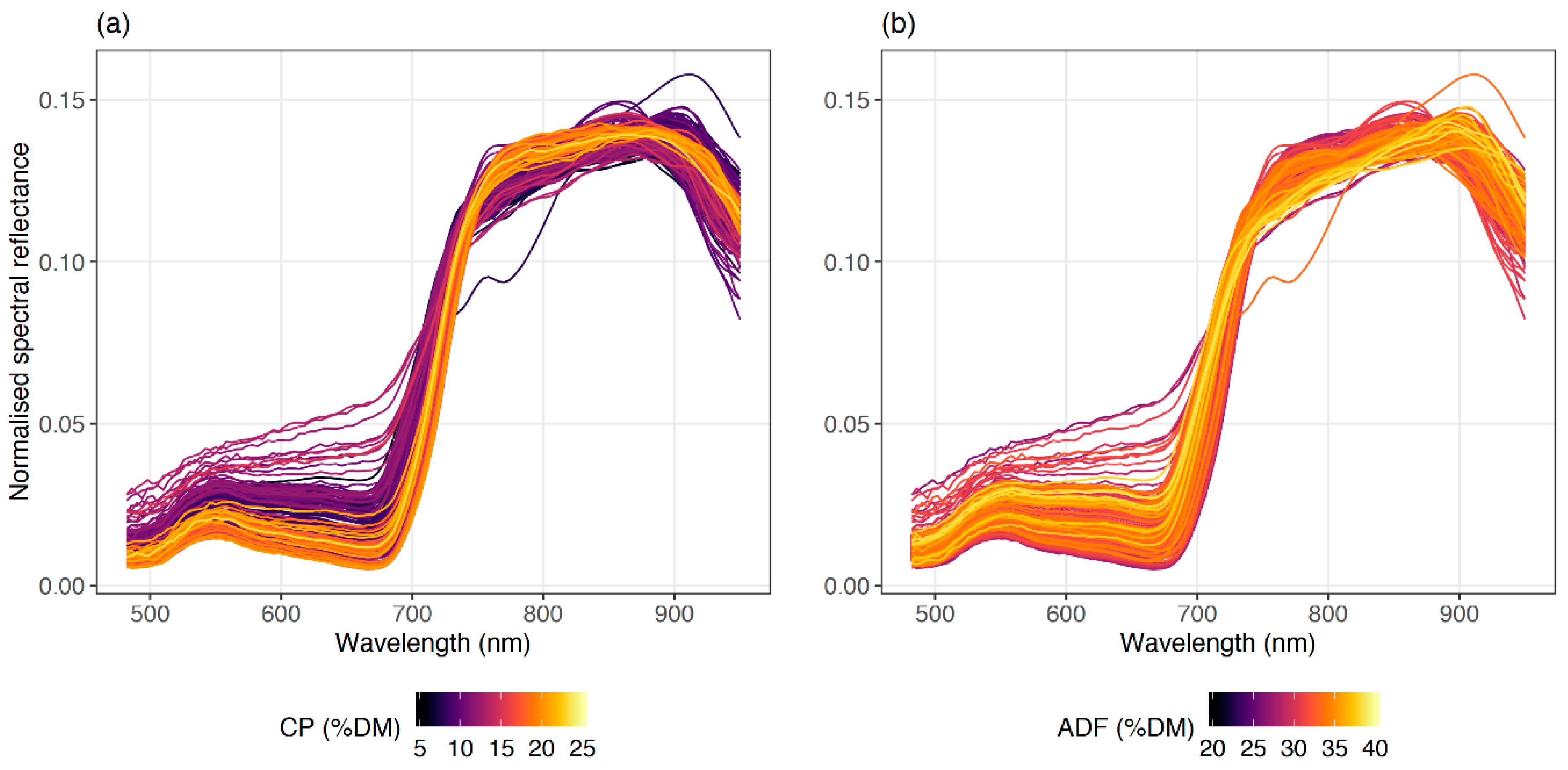
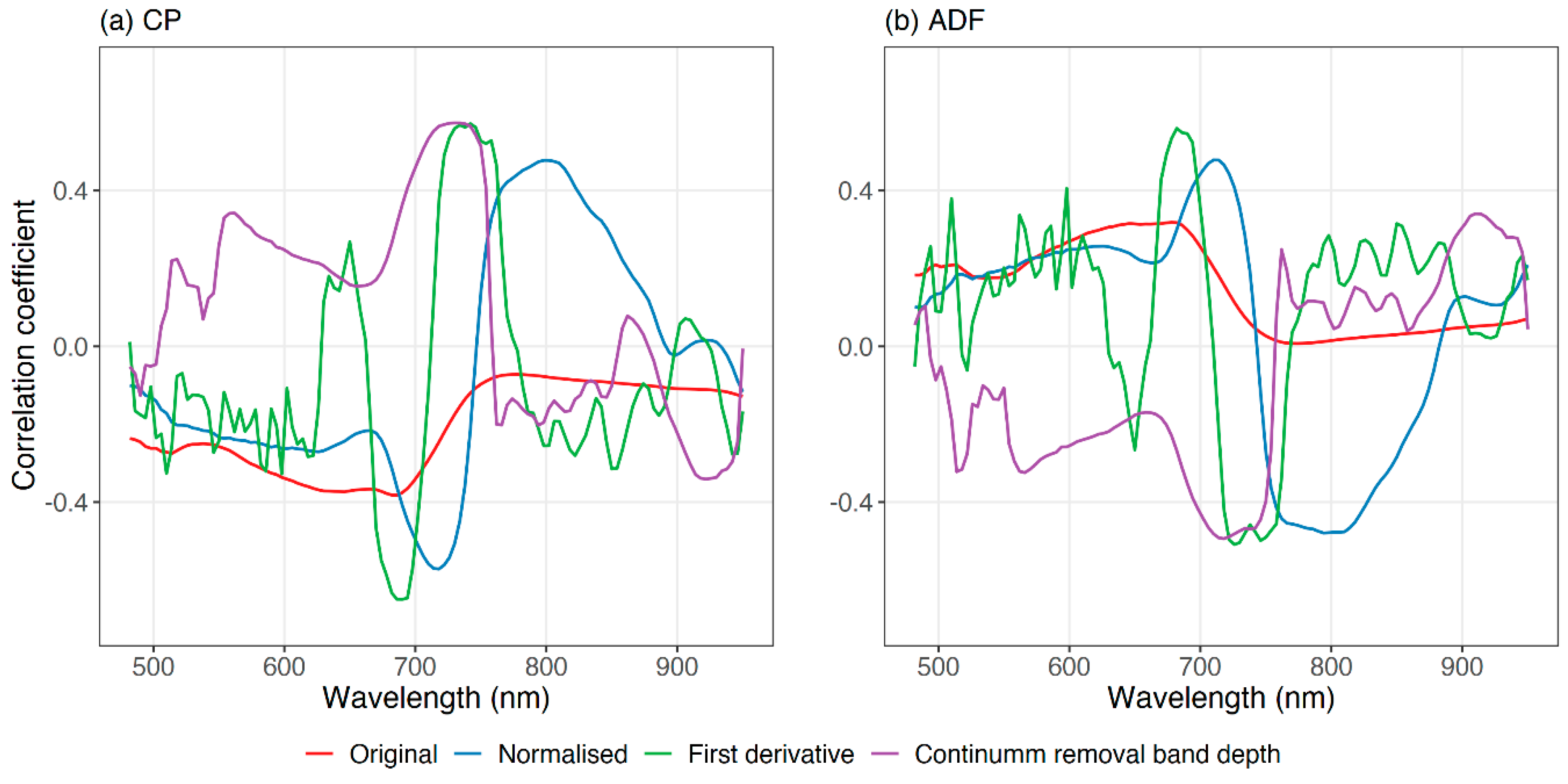
Correlograms were used to understand the relationship between grassland CP and ADF and spectral reflectance (Figure 7). For both quality parameters, normalised spectra indicated a stronger relationship with forage quality parameters than the original spectra or other spectra transformations (derivatives and continuum removal band depth). The normalisation process reduced the temporal noise of the data, which strengthened the relationship between spectral features and forage quality. Further, two correlograms from CP and ADF showed an inverse pattern, confirmed by the negative correlation between them. Nevertheless, both forage quality parameters had a stronger relationship in the red-edge and the near-infrared regions of the spectrum.

Linear regression models with spectral features (single waveband, NDSI, SR) obtained a maximum adj.R² of 0.42 for CP and 0.34 for ADF. The best correlated NDSIs comprised wavebands in the chlorophyll absorption features in the visible domain of the spectrum (470–518 nm and 550–750 nm), which relates to N and other biochemicals in green canopies [14]. These results paralleled with the results from previous studies that come from the same geographical region [15,18]. The study from Safari et al. [32] obtained linear regression models with NDSI with R² of 0.58 and 0.49 for CP and ADF, respectively. Moreover, the results from Biewer et al. [15] reported R² values of 0.33 and 0.13 R² for CP and ADF models with SR, respectively. Nonetheless, the results from the studies mentioned above were obtained with field spectroscopy data, which had a more comprehensive spectral range (305–1700 nm) than the camera utilised in the present study.

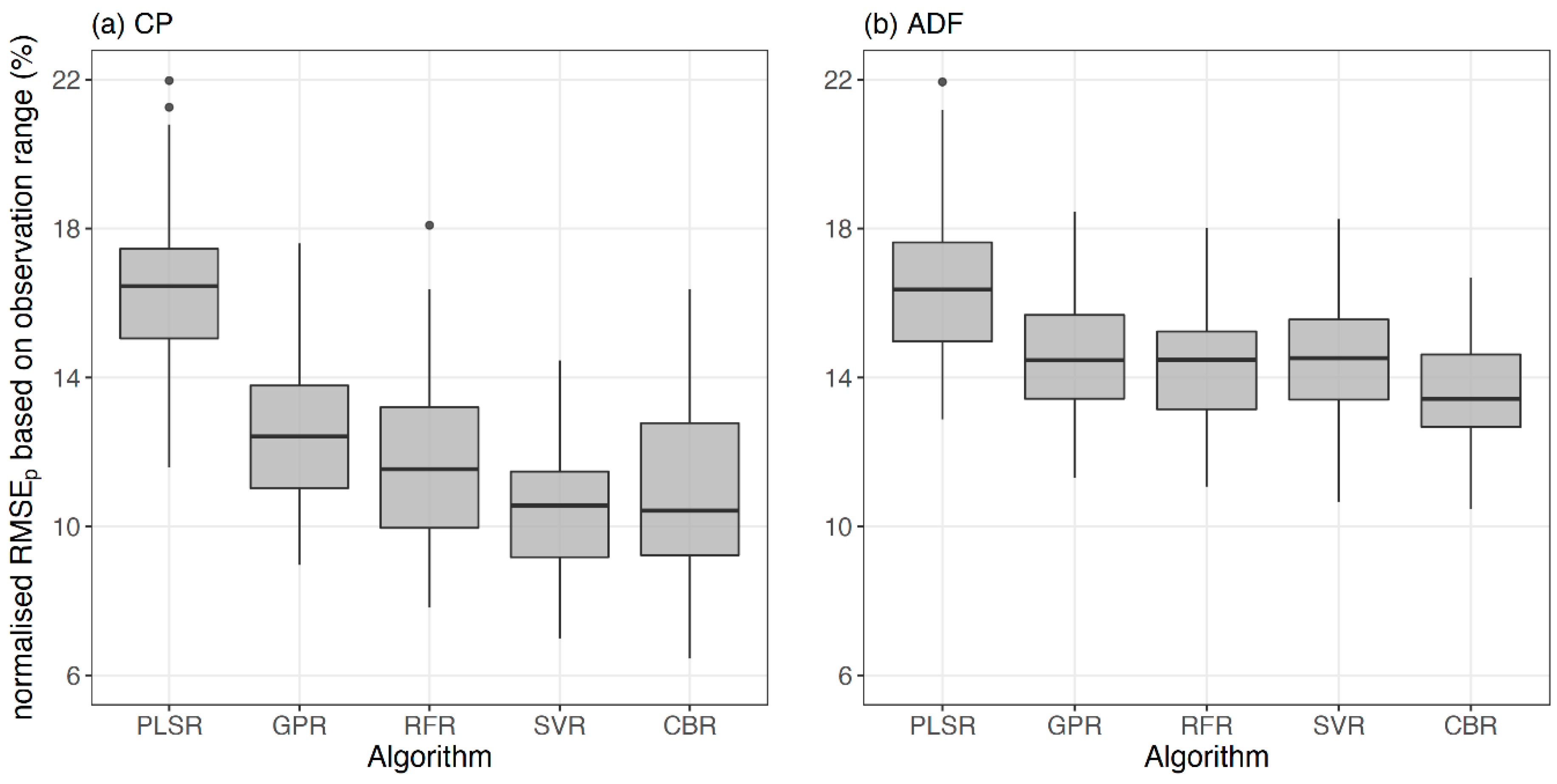
Several predictive modelling algorithms were tested to identify the best algorithms to estimate CP and ADF from the full spectral data, as no single consistent algorithm was shown to surpass all the given circumstances every time in a study by the authors of [61]. Moreover, model consistency was evaluated by training and testing 100 models using 100 different random train and test data sets, which allowed to disclose the model performance irrespective of the calibration data set. Except for the PLSR, other tested predictive algorithms (GPR, RFR, SVR, and CBR) proved promising for the underlying data. The SVR and CBR models for CP and ADF estimation showed the maximum precision (highest R²_p) and prediction accuracy (lowest nRMSE_p) followed by the RFR, GPR, and PLSR models, respectively. SVR and CBR predictive modelling algorithms were previously utilised to estimate water quality parameters based on spectral data [62,63], however, to our knowledge, such algorithms have not been employed so far to estimate forage quality parameters.

According to the literature, the PLSR and RFR were the most prominent predictive modelling algorithms in forage quality parameter estimation using spectral data. For example, Safari et al. (2016) report on PLSR models, which obtained nRMSE values of 8.5% and 7.3% for CP and ADF, respectively. However, PLSR models resulted in the lowest accuracies both for CP and ADF in this study. Moreover, Pullanagari et al. [34] achieved an nRMSE of 11.2% for CP with the RFR model, and Singh et al. [33] obtained an nRMSE of 21.7% for ADF with the same modelling algorithm. It is noteworthy that the studies mentioned above only tested one predictive modelling algorithm; thus, no conclusions are possible considering the comparison with other algorithms.

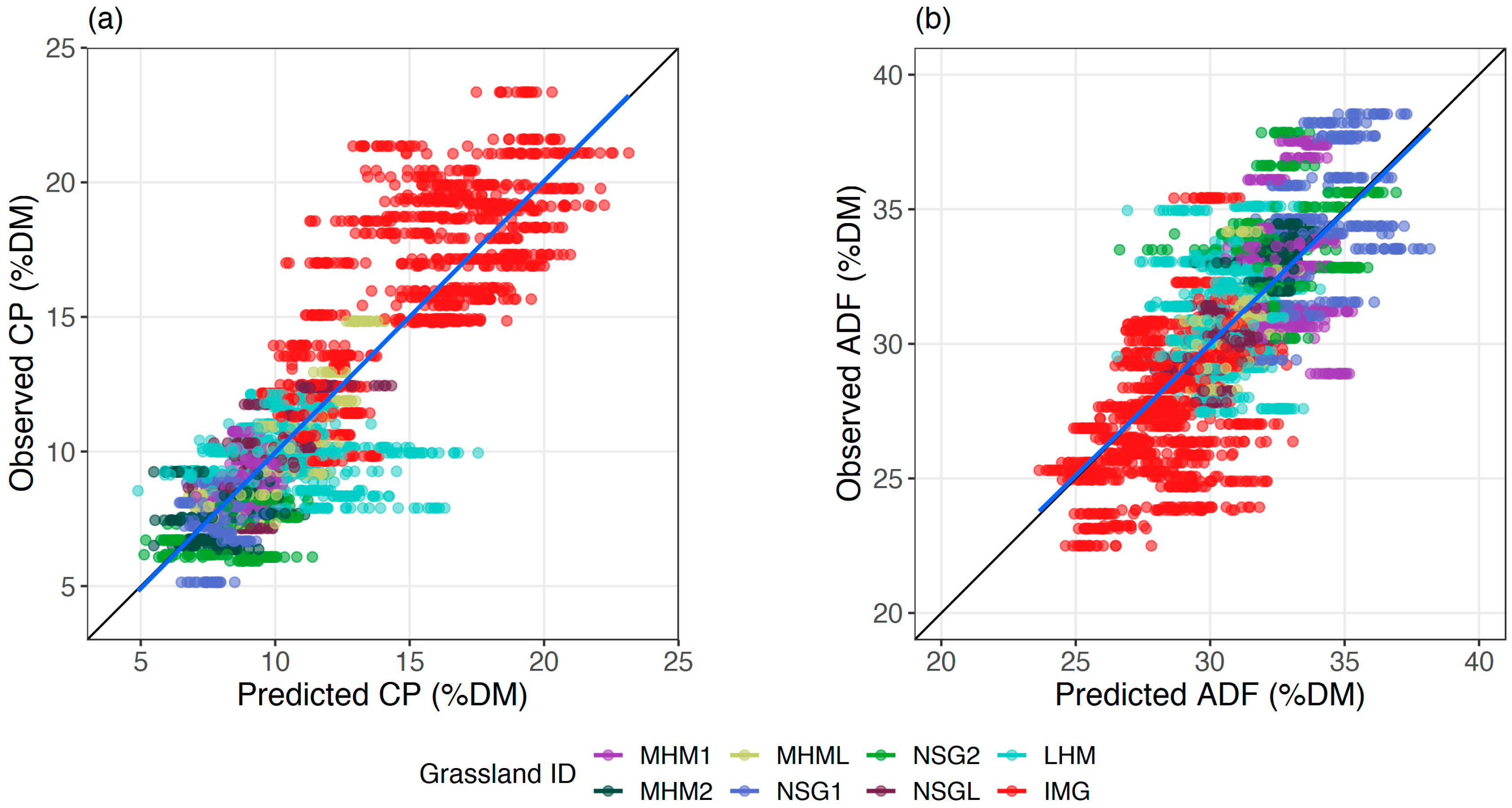
Both CP and ADF estimation models resulted in less than 15% relative prediction error. However, CP estimation had a slightly lower relative error (median nRMSE_p = 10.6%) than ADF estimation (median nRMSE_p = 13.4%). A similar relative error pattern for CP and ADF estimation models was obtained in previous studies that utilised field spectroscopy data [16,18,64]. Moreover, the data points from the IMG were clustered out and acted as the driver of the CP model according to the plot of fit (Figure 9a). 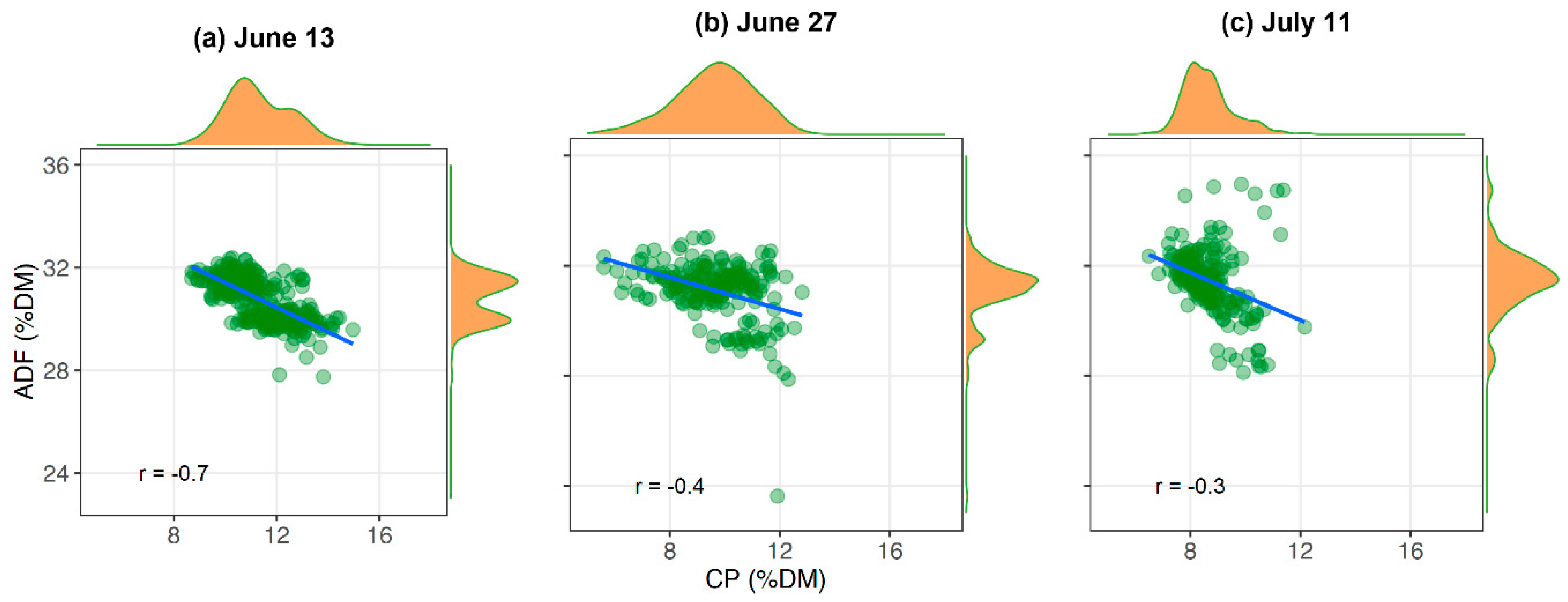Although, ADF data points in the observed against predicted plot did not highlight a similar pattern (Figure 9b). The high variation of CP between the cuts in IMG due to intensive management practice might be the reason for the mentioned pattern. However, the data points from other grasslands were mostly grouped in both plots because they almost experienced similar management practice.

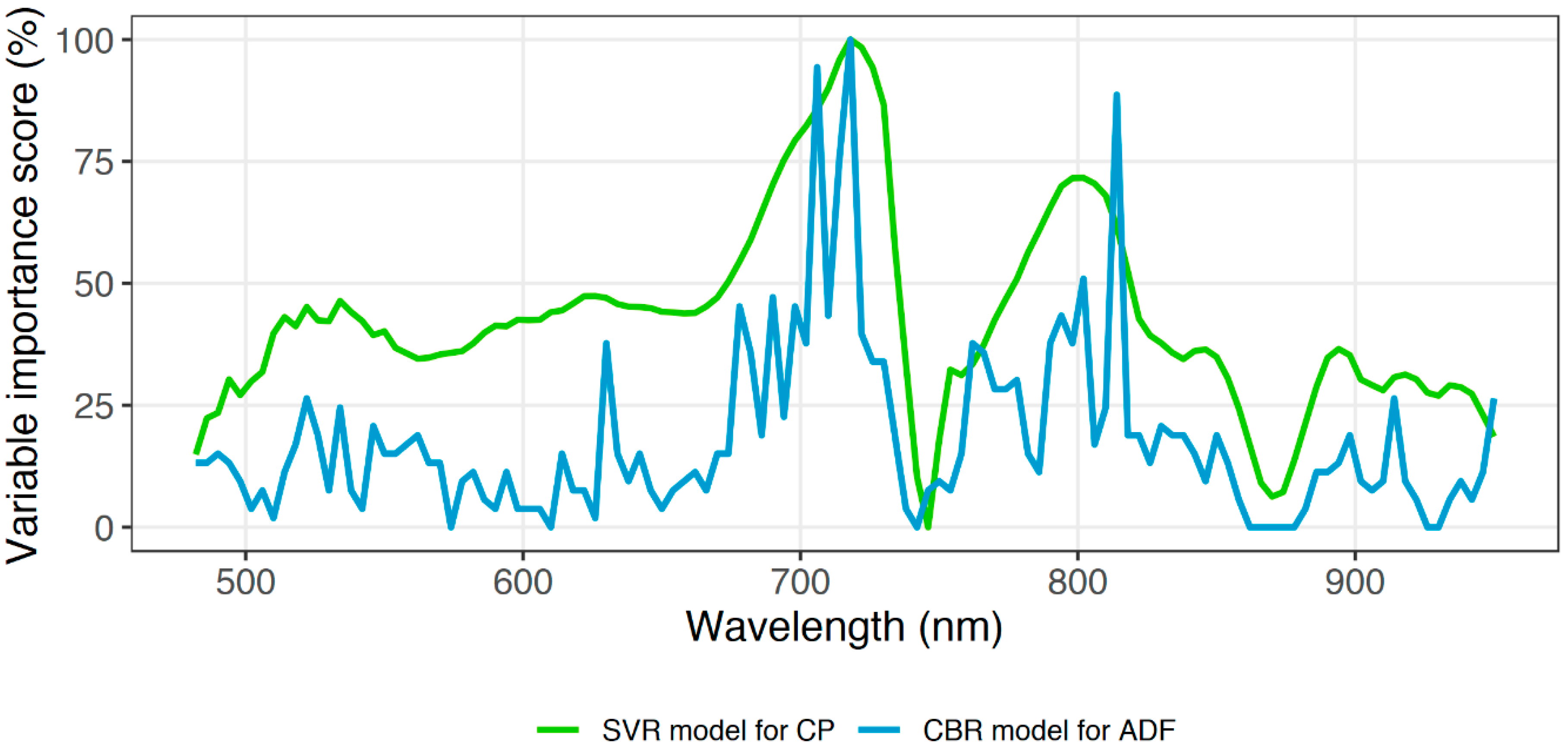
Remarkably, the wavelength (718 nm) that obtained the highest linear correlation with CP turned out to be the most fundamental wavelength for the final CP and ADF models (Figure A1). However, the identified first most important wavelengths were not related to any foliar chemical absorption feature, such as chlorophyll, protein, or cellulose [65]. According to Curran [65], the absorption features that relate to CP and ADF can be found at wavelengths in the shortwave infrared region of the spectrum (1400–3000 nm). Singh et al. [33] also confirmed that important wavelengths for ADF were in the shortwave infrared region of the spectrum. The camera used in the present study did not have the sensitivity to the shortwave infrared regions, even though the study showed a superior accuracy for grassland CP and ADF.

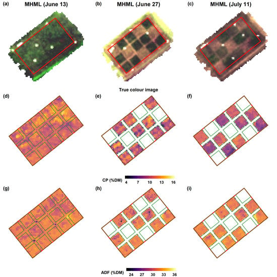
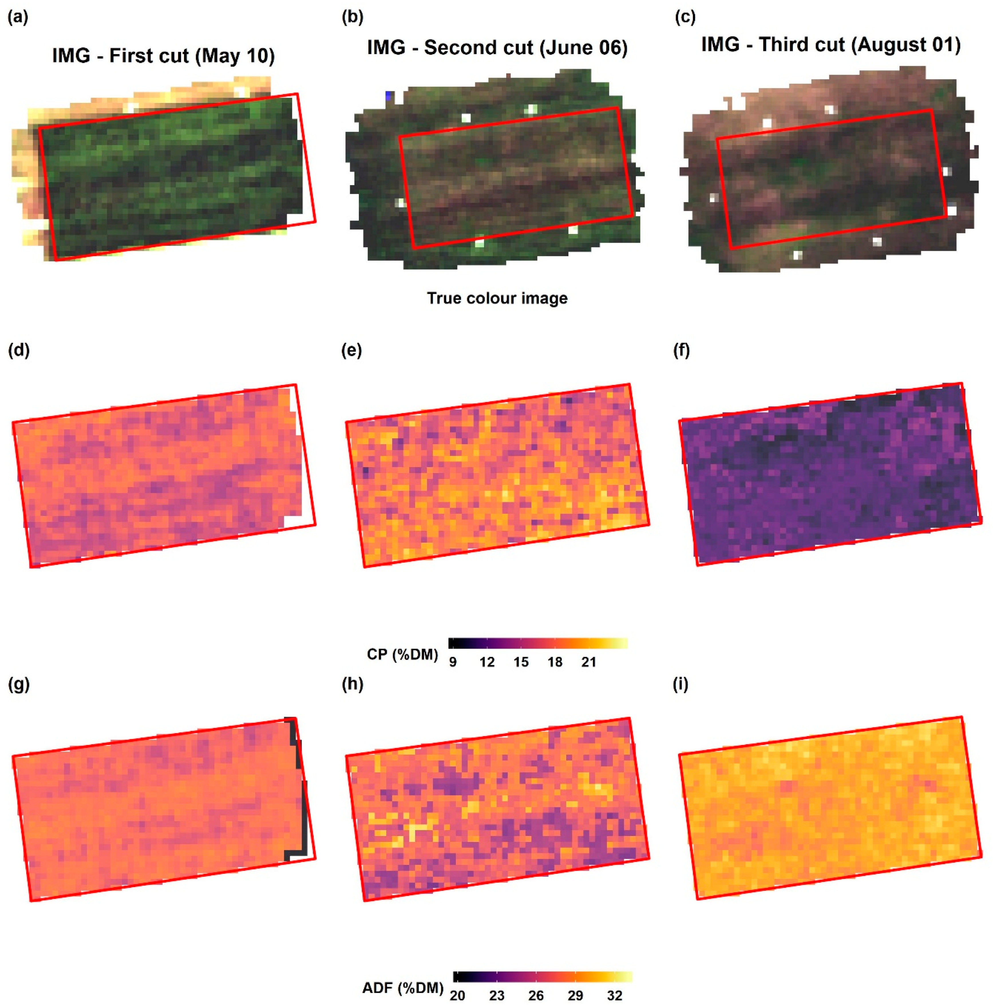
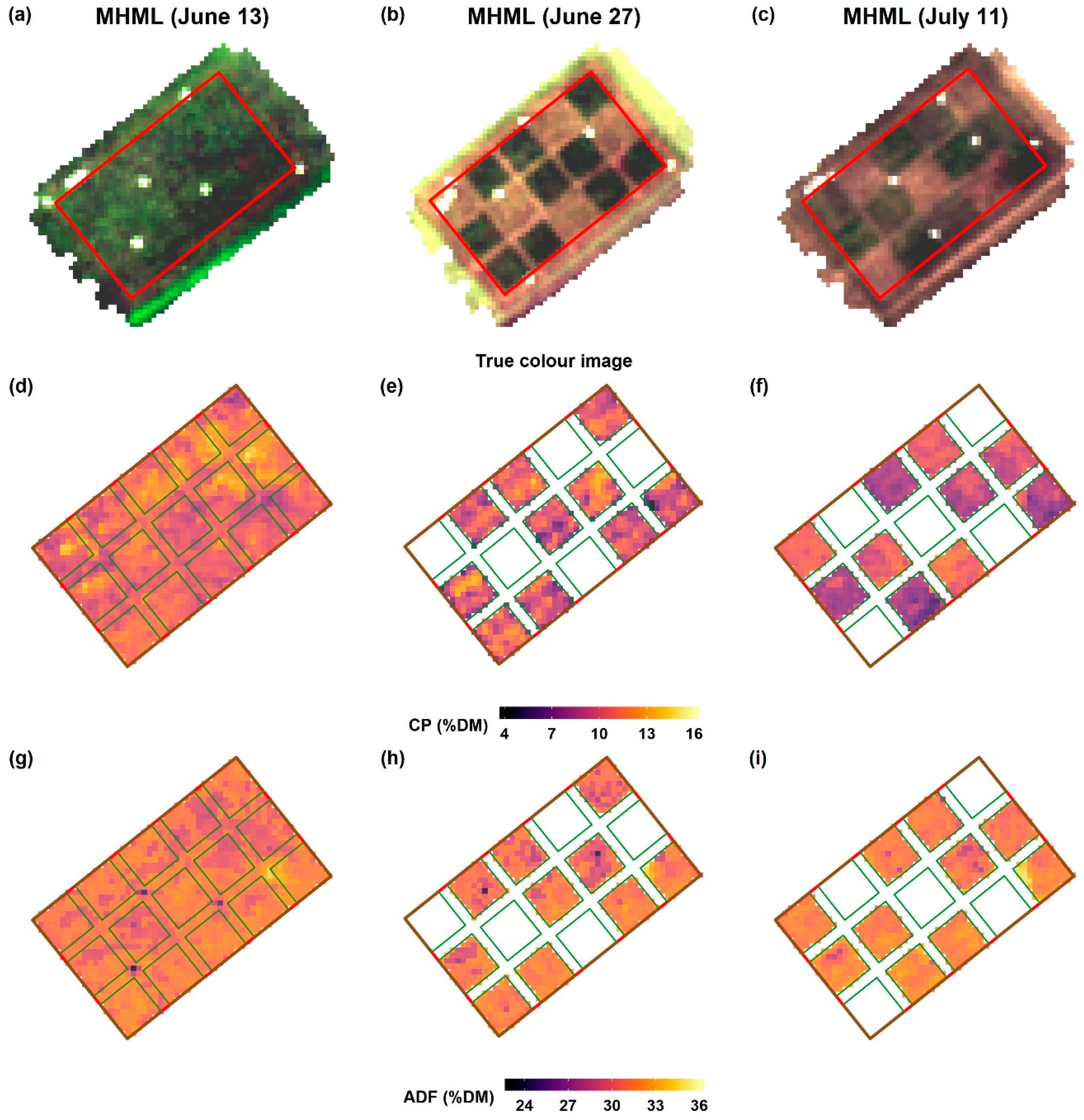
Imaging spectroscopy provides the advantage to generate maps by direct application of the model to recorded spectral images without the need for spatial interpolation. The prediction maps in our study displayed a substantial spatial variation in forage quality on the grasslands. While there is an inverse relationship between CP and ADF at the early cutting date of the MHML grassland, it vanishes with the increasing maturity of plants (Figure 12). Thus, biomass from such grasslands (MHML, NSGL) may display a much more considerable variation in CP than in ADF content, which probably depends very much on the degree of Lupinus polyphyllus invasion. Such information may help farmers to identify areas with contrasting forage quality, which is a prerequisite for targeted site-specific management of larger fields, for example, to determine a sound scheduling of mowing or grazing activities. Further, biomass from grassland areas with contrasting quality may be collected and ensiled separately to match the requirements of animals, which usually differ sharply among different animal species and performance categories.

To summarise, predictive modelling algorithms allow an adequate forage quality estimation, regardless of the grassland type and cutting regimes applied. Ultimately, fine-tuning of the calibrated models with data from further diverse grassland types could increase the robustness of the models to generate forage quality maps for grasslands with different vegetation types and management practices.

5. Conclusions

The present study aimed to estimate CP and ADF concentrations of a multitude of grasslands with different vegetation composition and cutting regimes applied based on UAV-borne imaging spectroscopy data. It was demonstrated that the resulting models could accurately estimate CP and ADF irrespective of the grassland type, and that model accuracies are in the same range as those obtained with the use of field spectroscopy. With such models, forage quality maps can be generated, which may provide a benefit for practical grassland farming. Eventually, continued tweaking of the models with data from additional grasslands will be a way forward to ultimately obtain an accurate generalised model with a validity range that covers most grasslands within a broader region.

References

1. Huyghe, C.; De Vliegher, A.; van Gils, B.; Peeters, A. Grasslands and Herbivore Production in Europe and Effects of Common Policies; Huyghe, C., De Vliegher, A., van Gils, B., Peeters, A., Eds.; Quae Editor: Versailles, France, 2014; ISBN 9782759221578. [Google Scholar]
2. Lesschen, J.P.; Elbersen, B.S.; Hazeu, G.W.; van Doorn, A.; Mucher, C.A.; Velthof, G.L. Defining and Classifying Grasslands in Europe—Task 1; Wageningen Environmental Research: Wageningen, The Netherlands, 2014. [Google Scholar]
3. t’Mannetje, L.; Jones, R. Field and Laboratory Methods for Grassland and Animal Production Research; t’Mannetje, L., Jones, R., Eds.; CABI Publishing: Oxon, UK, 2000; ISBN 0-85199-351-6. [Google Scholar]
4. Heather, R.; Nature, E. Grassland Monitoring. In Lowland Grassland Management Handbook; Crofts, A., Jefferson, R.G., Eds.; English Nature: Peterborough, UK, 1999; Volume 2, pp. 15:1–15:21. ISBN 1857164431. [Google Scholar]
5. Wachendorf, M. Advances in remote sensing for monitoring grassland and forage production. In Improving Grassland and Pasture Management in Temperate Agriculture; Marshal, A., Collins, R., Eds.; Burleigh Dodds Science Publishing: Cambridge, UK, 2018. [Google Scholar]
6. Horrocks, R.D.; Vallentine, J.F. Forage quality—the basics. In Harvested Forage; Horrocks, R.D., Vallentine, J.F., Eds.; Acdemic Press: San Diego, CA, USA, 1999; pp. 17–47. ISBN 9780977304561. [Google Scholar]
7. Gibson, D.J. Grasses and Grassland Ecology, 1st ed.; Oxford University Press: Oxford, UK, 2009; ISBN 9780198529187. [Google Scholar]
8. Frame, J.; Laidlaw, A.S. Feeding value of grass. In Improved Grassland Management; Frame, J., Laidlaw, A.S., Eds.; Corwood Press: Wiltshire, UK, 2011; pp. 167–180. ISBN 9781847972613. [Google Scholar]
9. Numata, I. Characterization on pastures using field and imaging spectrometers. In Hyperspectral Remote Sensing of Vegetation; Prasad, S.T., John, G.L., Alfredo, H., Eds.; CRC Press: Boca Raton, FL, USA, 2011; pp. 207–225. [Google Scholar]
10. Möckel, T. Hyperspectral and Multispectral Remote Sensing for Mapping Grassland Vegetation; Department of Physical Geography and Ecosystem Science, Lund University: Lund, Skåne, 2015; ISBN 978-91-85793-46-4. [Google Scholar]
11. Wachendorf, M.; Fricke, T.; Möckel, T. Remote sensing as a tool to assess botanical composition, structure, quantity and quality of temperate grasslands. Grass Forage Sci. 2017, 73, 1–14. [Google Scholar] [CrossRef]
12. Ali, I.; Cawkwell, F.; Dwyer, E.; Barrett, B.; Green, S. Satellite remote sensing of grasslands: From observation to management–A review. J. Plant Ecol. 2016, 9, 649–671. [Google Scholar] [CrossRef] [Green Version]
13. Milton, E.J. Principles of field spectroscopy. Int. J. Remote Sens. 1987, 8, 1807–1827. [Google Scholar] [CrossRef]
14. Mutanga, O.; Skidmore, A.K.; Prins, H.H.T. Predicting in situ pasture quality in the Kruger National Park, South Africa, using continuum-removed absorption features. Remote Sens. Environ. 2004, 89, 393–408. [Google Scholar] [CrossRef]
15. Biewer, S.; Fricke, T.; Wachendorf, M. Development of canopy reflectance models to predict forage quality of legume-grass mixtures. Crop Sci. 2009, 49, 1917–1926. [Google Scholar] [CrossRef]
16. Pullanagari, R.R.; Yule, I.J.; Tuohy, M.P.; Hedley, M.J.; Dynes, R.A.; King, W.M. In-field hyperspectral proximal sensing for estimating quality parameters of mixed pasture. Precis. Agric. 2012, 13, 351–369. [Google Scholar] [CrossRef]
17. Ramoelo, A.; Skidmore, A.K.; Schlerf, M.; Heitkönig, I.M.A.; Mathieu, R.; Cho, M.A. Savanna grass nitrogen to phosphorous ratio estimation using field spectroscopy and the potential for estimation with imaging spectroscopy. Int. J. Appl. Earth Obs. Geoinf. 2013, 23, 334–343. [Google Scholar] [CrossRef]
18. Safari, H.; Fricke, T.; Wachendorf, M. Determination of fibre and protein content in heterogeneous pastures using field spectroscopy and ultrasonic sward height measurements. Comput. Electron. Agric. 2016, 123, 256–263. [Google Scholar] [CrossRef]
19. Goetz, A.F.H.; Vane, G.; Solomon, J.E.; Rock, B.N. Imaging spectrometry for earth remote sensing. Science 1985, 228, 1147–1153. [Google Scholar] [CrossRef]
20. Skidmore, A.K.; Ferwerda, J.G.; Mutanga, O.; Van Wieren, S.E.; Peel, M.; Grant, R.C.; Prins, H.H.T.; Balcik, F.B.; Venus, V. Forage quality of savannas—Simultaneously mapping foliar protein and polyphenols for trees and grass using hyperspectral imagery. Remote Sens. Environ. 2010, 114, 64–72. [Google Scholar] [CrossRef]
21. Knox, N.M.; Skidmore, A.K.; Prins, H.H.T.; Asner, G.P.; van der Werff, H.M.; de Boer, W.F.; van der Waal, C.; de Knegt, H.J.; Kohi, E.M.; Slotow, R.; et al. Dry season mapping of savanna forage quality, using the hyperspectral Carnegie Airborne Observatory sensor. Remote Sens. Environ. 2011, 115, 1478–1488. [Google Scholar] [CrossRef]
22. Hakala, T.; Viljanen, N.; Honkavaara, E.; Näsi, R.; Niemeläinen, O.; Kaivosoja, J. A Novel Machine Learning Method for Estimating Biomass of Grass Swards Using a Photogrammetric Canopy Height Model, Images and Vegetation Indices Captured by a Drone. Agriculture 2018, 8, 70. [Google Scholar]
23. Capolupo, A.; Kooistra, L.; Berendonk, C.; Boccia, L.; Suomalainen, J. Estimating plant traits of grasslands from UAV-acquired hyperspectral images: A comparison of statistical approaches. ISPRS Int. J. Geo-Inf. 2015, 4, 2792–2820. [Google Scholar] [CrossRef]
24. Näsi, R.; Viljanen, N.; Kaivosoja, J.; Alhonoja, K.; Hakala, T.; Markelin, L.; Honkavaara, E. Estimating biomass and nitrogen amount of barley and grass using UAV and aircraft based spectral and photogrammetric 3D features. Remote Sens. 2018, 10, 1082. [Google Scholar] [CrossRef] [Green Version]
25. Wijesingha, J.; Moeckel, T.; Hensgen, F.; Wachendorf, M. Evaluation of 3D point cloud-based models for the prediction of grassland biomass. Int. J. Appl. Earth Obs. Geoinf. 2019, 78, 352–359. [Google Scholar] [CrossRef]
26. Grüner, E.; Astor, T.; Wachendorf, M. Biomass prediction of heterogeneous temperate grasslands using an SfM approach based on UAV imaging. Agronomy 2019, 9, 54. [Google Scholar] [CrossRef] [Green Version]
27. Durante, M.; Oesterheld, M.; Piñeiro, G.; Vassallo, M.M. Estimating forage quantity and quality under different stress and senescent biomass conditions via spectral reflectance. Int. J. Remote Sens. 2014, 35, 2963–2981. [Google Scholar] [CrossRef]
28. Castro, P.A.; Garbulsky, M.F. Spectral normalized indices related with forage quality in temperate grasses: Scaling up from leaves to canopies. Int. J. Remote Sens. 2018, 39, 3138–3163. [Google Scholar] [CrossRef]
29. Zengeya, F.M.; Mutanga, O.; Murwira, A. Linking remotely sensed forage quality estimates from worldview-2 multispectral data with cattle distribution in a savanna landscape. Int. J. Appl. Earth Obs. Geoinf. 2012, 21, 513–524. [Google Scholar] [CrossRef]
30. Starks, P.J.; Coleman, S.W.; Phillips, W.A. Determination of forage chemical composition using remote sensing. J. Range Manag. 2004, 57, 635–640. [Google Scholar] [CrossRef]
31. Ramoelo, A.; Skidmore, A.K.; Cho, M.A.; Mathieu, R.; Heitkönig, I.M.A.; Dudeni-Tlhone, N.; Schlerf, M.; Prins, H.H.T. Non-linear partial least square regression increases the estimation accuracy of grass nitrogen and phosphorus using in situ hyperspectral and environmental data. ISPRS J. Photogramm. Remote Sens. 2013, 82, 27–40. [Google Scholar] [CrossRef]
32. Safari, H.; Fricke, T.; Reddersen, B.; Möckel, T.; Wachendorf, M. Comparing mobile and static assessment of biomass in heterogeneous grassland with a multi-sensor system. J. Sens. Sens. Syst. 2016, 5, 301–312. [Google Scholar] [CrossRef] [Green Version]
33. Singh, L.; Mutanga, O.; Mafongoya, P.; Peerbhay, K. Remote sensing of key grassland nutrients using hyperspectral techniques in KwaZulu-Natal, South Africa. J. Appl. Remote Sens. 2017, 11, 036005. [Google Scholar] [CrossRef]
34. Pullanagari, R.R.; Kereszturi, G.; Yule, I. Integrating airborne hyperspectral, topographic, and soil data for estimating pasture quality using recursive feature elimination with random forest regression. Remote Sens. 2018, 10, 1117. [Google Scholar] [CrossRef] [Green Version]
35. Mutanga, O.; Skidmore, A.K. Integrating imaging spectroscopy and neural networks to map grass quality in the Kruger National Park, South Africa. Remote Sens. Environ. 2004, 90, 104–115. [Google Scholar] [CrossRef]
36. Aasen, H.; Burkart, A.; Bolten, A.; Bareth, G. Generating 3D hyperspectral information with lightweight UAV snapshot cameras for vegetation monitoring: From camera calibration to quality assurance. ISPRS J. Photogramm. Remote Sens. 2015, 108, 245–259. [Google Scholar] [CrossRef]
37. Cubert S185; Cubert GmbH: Ulm, Germany, 2016.
38. Copter Squad. RTK-X8 Hyperspectral Mapping; Cubert GmbH: Ulm, Germany, 2018. [Google Scholar]
39. Yang, G.; Li, C.; Wang, Y.; Yuan, H.; Feng, H.; Xu, B.; Yang, X. The DOM generation and precise radiometric calibration of a UAV-mounted miniature snapshot hyperspectral imager. Remote Sens. 2017, 9, 642. [Google Scholar] [CrossRef] [Green Version]
40. R Core Team. R: A Language and Environment for Statistical Computing; R Core Team: Vienna, Austria, 2019. [Google Scholar]
41. Hijmans, R.J. Raster: Geographic Data Analysis and Modelling; Tokyo, Japan, 2019. Available online: https://rdrr.io/cran/raster/ (accessed on 27 December 2019).
42. AgiSoft LLC. AgiSoft PhotoScan Professional 2018. Available online: https://www.agisoft.com/ (accessed on 27 December 2019).
43. Sun, L.; Wu, Z.; Liu, J.; Xiao, L.; Wei, Z. Supervised spectral-spatial hyperspectral image classification with weighted markov random fields. IEEE Trans. Geosci. Remote Sens. 2015, 53, 1490–1503. [Google Scholar] [CrossRef]
44. Dawson, T.P.; Curran, P.J. Technical note A new technique for interpolating the reflectance red edge position. Int. J. Remote Sens. 1998, 19, 2133–2139. [Google Scholar] [CrossRef]
45. Clark, R.N.; Roush, T.L. Reflectance spectroscopy: Quantitative analysis techniques for remote sensing applications. J. Geophys. Res. Solid Earth 1984, 89, 6329–6340. [Google Scholar] [CrossRef]
46. Geladi, P.; Kowalski, B.R. Partial least-squares regression: A tutorial. Anal. Chim. Acta 1986, 185, 1–17. [Google Scholar] [CrossRef]
47. Rasmussen, C.E.; Williams, C.K.I. Gaussian Processes for Machine Learning; The MIT Press: Cambridge, MA, USA, 2006; ISBN 026218253X. [Google Scholar]
48. Williams, C.K.I.; Rasmussen, C.E. Gaussian Processes for Regression; MIT Press: Cambridge, MA, USA, 2008. [Google Scholar]
49. Breiman, L. Random forests. Mach. Learn. 2001, 45, 5–32. [Google Scholar] [CrossRef] [Green Version]
50. Smola, A. Regression Estimation with Support Vector Learning Machines; Technische Universität München: Munich, Germany, 1996. [Google Scholar]
51. Drucker, H.; Burges, C.J.C.; Kaufman, L.; Smola, A.; Vapnik, V. Support vector regression machines. Fuzzy Sets Syst. 2003, 138, 271–281. [Google Scholar]
52. Smola, A.J.; Schölkopf, B. A tutorial on support vector regression. Stat. Comput. 2004, 199–222. [Google Scholar] [CrossRef] [Green Version]
53. Quinlan, J.R. Simplifying decision trees. Int. J. Hum. Comput. Stud. 1999, 51, 497–510. [Google Scholar] [CrossRef] [Green Version]
54. Quinlan, J.R. Learning with Continuous Classes, Proceedings of the AI’92, Hobart, Tasmania, 16–18 November 1992; Adams, A., Sterling, L., Eds.; World Scientific: Singapore, 1992. [Google Scholar]
55. Quinlan, J.R. Combining instance-based and model-based learning. In Proceedings of the Tenth International Conference on International Conference on Machine Learning, aAmherst, MA, USA, 27–29 June 1993; Kaufmann, M., Ed.; Morgan Kaufmann Publishers Inc.: San Mateo, CA, USA, 2006; Volume 93, pp. 236–243. [Google Scholar]
56. Kuhn, M.; Johnson, K. Applied Predictive Modelling; Springer: New York, NY, USA, 2013; ISBN 1461468485. [Google Scholar]
57. Raschka, S. Model evaluation, model selection, and algorithm selection in machine learning. Comput. Res. Repos. 2018, 1811, 12808. [Google Scholar]
58. Kuhn, M.; Wing, J.; Weston, S.; Williams, A.; Keefer, C.; Engelhardt, A.; Cooper, T.; Mayer, Z.; Kenkel, B.; The R Core Team; et al. Caret: Classification and Regression Training 2018; R Core Team: Vienna, Austria, 2018. [Google Scholar]
59. Kvalseth, T.O. Cautionary note about R2. Am. Stat. 1985, 39, 279–285. [Google Scholar]
60. Otto, S.A. How to normalize the RMSE. Available online: https://www.marinedatascience.co/blog/2019/01/07/normalizing-the-rmse/ (accessed on 30 May 2019).
61. Yuan, H.; Yang, G.; Li, C.; Wang, Y.; Liu, J.; Yu, H.; Feng, H.; Xu, B.; Zhao, X.; Yang, X. Retrieving soybean leaf area index from unmanned aerial vehicle hyperspectral remote sensing: Analysis of RF, ANN, and SVM regression models. Remote Sens. 2017, 9, 309. [Google Scholar] [CrossRef] [Green Version]
62. Hafeez, S.; Wong, M.; Ho, H.; Nazeer, M.; Nichol, J.; Abbas, S.; Tang, D.; Lee, K.; Pun, L. Comparison of machine learning algorithms for retrieval of water quality indicators in case-II waters: A case study of Hong Kong. Remote Sens. 2019, 11, 617. [Google Scholar] [CrossRef] [Green Version]
63. Keller, S.; Maier, P.M.; Riese, F.M.; Norra, S.; Holbach, A.; Börsig, N.; Wilhelms, A.; Moldaenke, C.; Zaake, A.; Hinz, S. Hyperspectral data and machine learning for estimating CDOM, chlorophyll a, diatoms, green algae and turbidity. Int. J. Environ. Res. Public Health 2018, 15, 1881. [Google Scholar] [CrossRef] [Green Version]
64. Kawamura, K.; Watanabe, N.; Sakanoue, S.; Inoue, Y. Estimating forage biomass and quality in a mixed sown pasture based on partial least squares regression with waveband selection. Grassl. Sci. 2008, 54, 131–145. [Google Scholar] [CrossRef]
65. Curran, P.J. Remote sensing of foliar chemistry. Remote Sens. Environ. 1989, 30, 271–278. [Google Scholar] [CrossRef]
Figure 1. Map of Germany (a) and the areas with the location of grasslands investigated in the study (b,c). MHM, mountain hay meadow; NSG, Nardus stricta grassland. MHML, MHM invaded by Lupinus polyphyllus; NSGL, NSG invaded by Lupinus polyphyllus; LHM, lowland hay meadow; IMG, intensively managed grassland.
Remotesensing 12 00126 g001
Figure 2. The unmanned aerial vehicle (UAV) and the Cubert camera used in the study.
Remotesensing 12 00126 g002
Figure 3. The workflow for processing the UAV-borne spectral images to obtain a single geo-referenced ortho-mosaic.
Remotesensing 12 00126 g003
Figure 4. The model building workflow. (PLSR: partial least squares regression, RFR: random forest regression, GPR: Gaussian processes regression, SVR: support vector regression, CBR: cubist regression, nRMSE: normalised RMSE).
Remotesensing 12 00126 g004
Figure 5. Distribution of crude protein (CP) (a) and acid detergent fibre (ADF) (b) concentrations in the harvested biomass of different grasslands.
Remotesensing 12 00126 g005
Figure 6. Normalised mean spectral reflectance for CP (a) and ADF (b) concentration data for all 1 m2 sampling plots.
Remotesensing 12 00126 g006
Figure 7. Correlogram for CP (a) and ADF (b) between original, normalised, derivative reflectance, and continuum removal band depth data.
Remotesensing 12 00126 g007
Figure 8. Normalised RMSEp distribution for CP (a) and ADF (b) concentrations in different grasslands for each predictive algorithm model (CBR: cubist regression, GPR: Gaussian processing regression, PLSR: partial least squares regression, RFR: random forest regression).
Remotesensing 12 00126 g008
Figure 9. Observation versus prediction scatter plots from the SVR model for CP (a) and the CBR model for ADF (b) concentrations in different grasslands. Colours represent different grasslands. The black line is the 1:1 line, and the blue line represents the linear regression line between observed and predicted values.
Remotesensing 12 00126 g009
Figure 10. Forage quality prediction maps for the intensively managed grassland (IMG). The first row is the hyperspectral mosaic in the true colour composite (R: 606 nm, G: 546 nm, B: 482 nm) for different sampling dates (ac). Predicted CP and ADF maps are shown in the second (df) and third rows (gi), respectively. Columns represent different cutting dates. The value range in the colour scale is different for each quality parameter. White spots in the map represent no data pixels.
Remotesensing 12 00126 g010
Figure 11. Forage quality prediction maps for the mountain hay meadow invaded by Lupinus polyphyllus (MHML). The first row is the hyperspectral mosaic in the true colour composite (R: 606 nm, G: 546 nm, B: 482 nm) for different sampling dates (ac). Predicted CP and ADF maps are shown in the second (df) and third rows (gi), respectively. Columns represent different cutting dates. The value range in the colour scale is different for each quality parameter. White spots in the map represent no data pixels. The 64 m2 small plot boundaries are in green colour.
Remotesensing 12 00126 g011
Figure 12. Scatter plots between predicted CP and ADF from MHML’s small plots harvested on 13 June (a), 27 June (b), and 11 July (c). The marginal histogram shows the distribution of each axis value.
Remotesensing 12 00126 g012