Abstract
It is very difficult and complex to acquire photosynthetic vegetation (PV) and non-PV (NPV) fractions (fPV and fNPV) using multispectral satellite sensors because estimations of fPV and fNPV are influenced by many factors, such as background-noise interference of pixel-, spatial-, and spectral-scale effects. In this study, comparisons between Sentinel-2A Multispectral Instrument (S2 MSI), Landsat-8 Operational Land Imager (L8 OLI), and GF1 Wide Field View (GF1 WFV) sensors for retrieving sparse photosynthetic and non-photosynthetic vegetation coverage are presented. The analysis employed a linear spectral-mixture model (LSMM) and nonlinear spectral-mixture model (NSMM) to unmix pixels with different spectral and spatial resolution images based on field endmembers; the estimated endmember fractions were later validated with reference to fraction measurements. The results demonstrated that: (1) with higher spatial and spectral resolution, the S2 MSI sensor had a clear advantage for retrieving PV and NPV fractions compared to L8 OLI and GF1 WFV sensors; (2) through incorporating more red edge (RE) and near-infrared (NIR) bands, the accuracy of NPV fraction estimation could be greatly improved; (3) nonlinear spectral mixing effects were not obvious on the 10–30 m spatial scale for desert vegetation; (4) in arid regions, a shadow endmember is a significant factor for sparse vegetation coverage estimated with remote-sensing data. The estimated NPV fractions were especially affected by the shadow effects and could increase root mean square by 50%. The utilized approaches in the study could effectively assess the performance of major multispectral sensors to extract fPV and fNPV through the novel method of spectral-mixture analysis.
1. Introduction
Arid regions occupy over 30% of the global land surface, and desertification is especially severe in arid and semiarid zones, affecting more than two billion people. In arid regions, degradation of natural vegetation is a serious issue since it causes wind augmentation and sand invasion, and greatly endangers the ecological environment. Photosynthetic vegetation (PV) is defined as plant material including chlorophyll (e.g., green leaves and flowers), which is a significant plant factor in arid and semiarid regions. Non-photosynthetic vegetation (NPV) is plant material lacking chlorophyll (e.g., senescent plants, branches, and plant stubble), and it occupies a great part of natural vegetation in arid and semiarid regions [1,2]. PV and NPV are not only important indicators for changes of the ecological environment, but are also essential elements in surveying vegetation status and researching carbon storage in arid regions [3]. Therefore, acquiring fractional cover of PV (fPV) and NPV (fNPV) data synchronicity and quantification is very significant for vegetation productivity and the monitoring of desertification. It also provides important factors for different ecological and hydrological models.
Remote-sensing technology has substantial capacity for the precise estimations of the fPV and fNPV of desert vegetation. The PV fraction is obtained from optical sensors using the red–near-infrared (NIR) band that can capture vegetation health status [4,5,6]. It is more challenging to determine the landscape percentage that is taken up by NPV, and especially to distinguish between dry plants and soil litter [7]. However, it is possible to differentiate components by spectral characteristics of lignin–cellulose between 2000 and 2200 nm with hyperspectral sensors [8,9,10]; limited data coverage and acquisition, however, cannot meet the demands of large-scale vegetation monitoring [11,12,13]. In contrast, multispectral sensors, despite lacking these spectral characteristics, have the advantage of large-scale spatial resolution, so they have been more utilized to retrieve NPV coverage [14,15,16]. Sensor capability generally constrains vegetation indices estimated from multispectral satellite data for PV and NPV mapping, mostly due to available sensors not being specifically designed for NPV calculations. Spectral-mixture analysis (SMA) provides an adequate method to calculate fPV and fNPV [2,17,18]. SMA commonly include two types depending on whether it focuses on multiple scattering or not. One is a broadly employed, namely linear SMA (LSMA), where a mixed spectrum is expressed as a linear relation to the pure spectrum of its elements. It is then weighted by the proportion of its subpixels without undertaking multiple scattering between possible components [19,20]. The second is nonlinear SMA (NSMA), which consists of multiple scattering between components [21,22,23]. These techniques could be utilized to analyze the spectral-mixture process of PV and NPV, thus allowing us to compare the capability of different multispectral sensors to calculate fPV and fNPV.
The new generation of satellites, characterized by additional spectral bands, especially in the red edge (RE) and shortwave infrared (SWIR), with higher spatial resolution or temporal frequency, have become operational during the last few years [24]. Compared to the novelty of these sensors, the potential for estimating fPV and fNPV in arid regions has not yet been fully explored. Therefore, we selected three major multispectral satellites in orbit with different spatial and spectral resolutions, Sentinel-2A Multispectral Instrument (S2 MSI), Landsat-8 Operational Land Imager (L8 OLI), and GF1 Wide Field View (GF1 WFV), to carry out fPV and fNPV estimation with SMA and comprehensively compare their performance. We had the following objectives: to test 1) whether the new bands could improve fPV and fNPV estimation accuracy in arid regions and 2) whether the spectral-mixing mechanism (linear or nonlinear) between PV, NPV, and others stayed consistent across spatial and spectral scales. In total, 111 field sites were selected in western China, and the coverage of PV–NPV–BS and the spectra of all surface types were measured. Satellite data, including Sentinel-2A MSI (10/20/60 m, 13-band), Landsat-8 OLI (30 m, MSI 7-band) and GF1-WFV (16 m, 4-band), with near-simultaneous acquisition were downloaded to estimate the fPV and fNPV with field-measured data. This research aims to provide new knowledge regarding comparisons of S2-MSI, L8 OLI, and GF1 WFV for retrieving fPV and fNPV in arid regions.
2. Materials and Methods
2.1. Study Area
The study was carried out at 38°37′42.60″N, 102°55′11.25″E, a transitional oasis and desert zone in the county of Minqin in China. It is situated at the overlap between the Tengri desert and the Cartap Jilin desert border down the Shiyang river. The area of the zone is 22.8 km2, and it is a semi-enclosed inland desert [25]. Natural plants are primarily composed of a few species of different types of desert vegetation, and there is apparent structure and low productivity, e.g., Haloxylon ammodendron and Nitraria tangutorum shrubs.
2.2. Field Measurement
2.2.1. Fractional-Cover Field Measurement
There were 111 surveyed fractional-cover sites with field measurements in August 2016 at Minqin (Figure 1). The central position of each field site was recorded by Global Positioning System (GPS) with a WGS84 coordinate system (Figure 2a–c). Following Guerschman, and Muir et al. [17,26], for natural or pastoral vegetation communities, field measurements use three 30 m measuring tapes cross-distributed in a hexagonal shape at intervals of 60 degrees from the midpoint (Figure 2d,e). For artificial vegetation in parallel rows, two 30 m tapes, orienting at 45 degrees and crossing the sowing lines, were used (Figure 2f,g). The observer recorded the type of material at each meter, including the amount of green leaves, cryptogams, dry leaves, and different kinds of bare soil, such as crust and rocks. If there was middle (shrub)- and/or upper-layer (tree) vegetation, it recorded top-layer coverage by looking up the meter point. The cover percentage was calculated by dividing the count for a special type by the total count (90 or 60). When records included plants with leaves still attached, the operator evaluated if it was photosynthetic vegetation on the basis of its colorings.
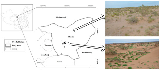
Figure 1.
Spatial distribution and pictures of field-observation locations.
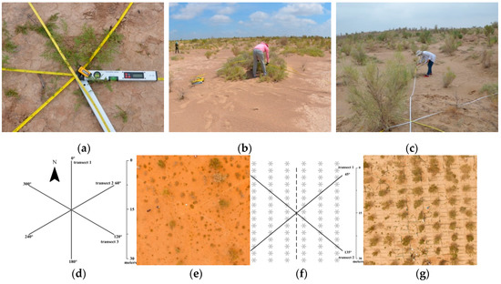
Figure 2.
Field observations. (a) Recording central location by Global Positioning System (GPS); (b,c) field measurements of vegetation fractional cover; (d) transect layout in natural or pastoral environments; (e,g) field-observation-site images taken by unmanned aerial vehicle (UAV) from natural environment and artificial vegetation in rows, respectively; (f) transect layout in artificial vegetation in rows.
2.2.2. Endmember Collection, Processing, and Selection
All endmember spectra were acquired by a portable Analytic Spectral Device (ASD; Boulder, CO, USA) spectroradiometer on 3–9 August 2016 in the field. A variety of PV, NPV, BS, and shadow endmember reflectance spectral measurements were acquired in full range (350–2500 nm). The ASD Spec Pro Field spectroradiometer with a 25° field-of-view angle took the measurements within 2 h of local solar noon. A white spectral panel was used to calibrate reflectance (Labsphere Inc., North Sutton, NH, USA). On a windless and sunny day, endmember spectra were continuously collected during 10:00–14:00. In order to obtain pure PV and NPV endmember canopy spectra, either full- absorption black cloth was laid at the bottom of the endmember canopy, or parts of the endmember material were placed on the black background. Meanwhile, probes were placed above all typical species’ endmember surfaces, from 0.1 to 0.02 m. In this way, we built the pure endmember spectral library from each field as shown in Figure 3. In view of endmember applicability and representativeness, it was required that the number of each endmember spectrum was no less than 10. A total of 84 reflectance spectra were collected, varying by 65 types of PV, 12 types of NPV, 10 types of bare soil, and 2 types of shadow (Figure 3).
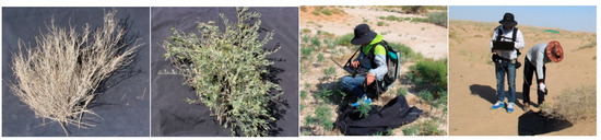
Figure 3.
Photosynthetic and non-photosynthetic vegetation (PV, NPV) endmember-spectrum collection in Minqin, China. Different protocols tested for endmember-spectrum acquisition. Process of excising PV or NPV canopy either placed on black background or directly placing black cloth under their canopy, then completely covering soil ground to ensure endmember-spectrum purity.
2.3. Satellite Data and Preprocess
For each Landsat-8 observation, GF1 and cloud free Sentinel-2 images were downloaded on the date closest to field-measurement dates within ±10 day discrepancy between field-measurement date and satellite acquisition date. Ground measurements for endmember spectra and reference fractions were considered for acquired-image data for Landsat-8, GF1, and Sentinel-2A sensors, as is shown in Table 1.

Table 1.
Sensor characteristics of Sentinel-2A Multispectral Instrument (S2 MSI), Landsat-8 Operational Land Imager (L8 OLI), and GF1 Wide Field View (GF1 WFV) imagery. Panchromatic and thermal bands not included.
The geometrically corrected Level-1C product S2 MSI image was downloaded from the Sentinels Scientific Data Hub (https://scihub.copernicus.eu/). Then, radiometric calibration and atmospheric correction are applied to the Level-1C images with the Sentinel Application Platform (SNAP) version 4.0.2 with Sen2Cor version 2.3.0 software, and SNAP with default parameter settings, was used to obtain surface-reflectance images of the study sites. S2 MSI includes 13 spectral bands: 4 bands at 10 m (blue, green, red, and NIR-1), 6 bands at 20 m (RE 1 to 3, NIR-2, SWIR 1 and 2) and 3 additional bands at 60 m spatial resolution. For our study, we adopted all effective bands for vegetation having 10 and 20 m resolution, and bands 11 and 12 with 60 m spatial resolution, excluding bands 1 and 10. The 20 m bands were resampled into 10 spatial resolution, and 60 m bands upscaled to 10 m spatial resolution according to experiment design with the nearest-neighbor resampling method by Data Management Tools (ARCGIS 10.3).
One Landsat-8 image (path 132, row 33), captured concurrently with the field campaign, was downloaded from the United States Geological Survey (USGS) Earth Explorer database (http://earthexplorer.usgs.gov). This was radiometrically calibrated and geometrically corrected, and then standardized to a nadir view by Environment for Visualizing Images software (ENVI 5.3). Landsat-8 OLI is a multispectral scanning device with 9 spectral bands. Band 1, band 8 pan and band 9 (shortwave infrared channel) were removed prior to this analysis because they are used to detect coastal zones and cirrus clouds. The image was spectrally corrected to reflectance in ENVI 5.3 using the calibration tool and Fast Line-of-sight Atmospheric Analysis of Spectral Hypercubes (FLAASH).
The GF-1 WFV image included only 4 bands that were 3 visible (VIS) wavebands and 1 near-infrared waveband. On account of its wide coverage, and high temporal and spatial resolution, it is an effective data source for the dynamic monitoring of large-scale vegetation coverage. GF1-WFV data covering the study area were provided by the China Center for Resource Satellite Data and Application (CRESDA, http://www.cresda.com/). Radiometric correction and atmospheric correction for GF1-WFV were achieved by ENVI 5.3 and the FLAASH algorithm, thus, radiance was transformed to surface reflectance. Then, the base map for geometric correction was Sentinel 2A, and geometric co-registration error was less than one pixel that of the Sentinel 2A data (10 m). All images are projected in the UTM projection and WGS84 geodetic system.
3. Method
Three commonly used multi-spectral sensors were compared to retrieve the fPV and fNPV in arid regions by employing linear spectral-mixture model and non-linear spectral-mixture model, mainly focusing on the effects of additional spectral bands, different spatial resolution, non-linear spectral mixture process and appropriate endmember identification. Field spectra data for vegetation, soil and shadow were collected for providing endmember spectra. Field-measured data for fPV and fNPV were acquired from the sample investigation, which were utilized for evaluating the performance of different models as a validation dataset. The flowchart of this study illustrates in Figure 4.
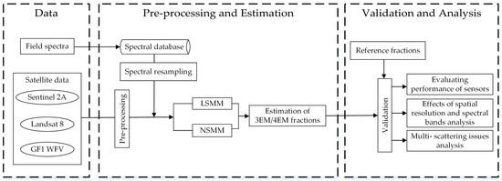
Figure 4.
Workflow diagram of methodology and analysis process.
3.1. Linear Spectral-Mixture Analysis
The linear spectral-mixture model (LSMM) is a broadly used method to unmix multicomponent composition in remote-sensing imagery. It assumes each incident photon passed only one reflection from the surface, without multiple scattering before entering the sensor [27,28]. A mixed pixel in LSMM (Equation (1)) is linear combination of endmember sets [4,29,30,31,32,33,34]. In general, the LSMM is
where Ri and Wi,j are the measured mixed reflectance and the jth endmember reflectance in band i, respectively; fj indicates the jth endmember fraction in the mixed pixel; and m indicates the number of endmembers. The work was conducted under the constrained condition of for j = 1, …, m (ANC) and (ASC); through Equation (1), fully constrained least-squares (FCLS) [35,36] was applied to calculate fj, for which we simplified the following equation:
where n indicates the number of valid wavebands, and. indicates the equation residual. In order to achieve ASC, new signature matrices M and F were introduced, defined as
With , and a vector F by
In Equations (3) and (4), δ represents a contribution factor weighted to the ratio of the sum to one constraint, and m represents the number of endmembers.
Non-negatively constrained least squares (NCLS) constrained the cover fraction with ANC. The iteration technique [35] was employed by leading a Lagrange multiplier vector (λ) into Equations (5) and (6) generating consequence
Temporal variation in shadow fractions under various solar illuminations can offer a trade-off between shadow fraction and other endmember fractions. Normalizing complementary fractions can remove shadow fractions. We normalized the shadow contribution by the following equation [27]:
where fj represents the jth endmember fraction in a mixed pixel except for shadow endmembers, and fshadow represents the shadow fraction.
3.2. Nonlinear Spectra-Mixture Model (NSMM)
Attributing to various NSMMs [37], it was recommended to use a kernel-function-based NSMM (KNSMM) in the study.
3.2.1. Kernel Method
The KNSMM generalizes the linear mixing model by introducing nonlinearities through kernel functions, so that vector Rn is represented in high-dimensional feature space C. Considering nonlinear mapping, , where the vector Rn illustrates the nonlinear relationship between the data with n dimensions, the feature space C shows a linear relationship in high-dimensional space. The equation illustrates that the nonlinear relationship between the original endmember spectral wavebands with high-order multiplications is transformed into a linear relationship in a high dimensional space by the nonlinear mapping . Thus, the KSMM includes linear ingredients in the feature space, and additive nonlinear ingredients in the primitive space [34,38,39,40].
Nonlinear mapping is usually uncertain and perhaps complex. Kernel-based learning algorithms employ kernel functions to achieve dot products for kernel function, illustrated as [41]
where xi and xj note the spectral value of the ith and jth endmember, respectively. The nonlinear relationship between xi and xj will be replaced by and with the nonlinear kernel function K(xi, xj) in the process. In theory, kernel functions comply to Mercer’s theorem [42,43]: “A Mercer kernel is symmetric (K(xi, xj) = K(xj, xi)) and positive definite ((K(xi, xj) >0))” [42,44]. According to our research objective, the radial-basis-function (RBF) kernel was applied because it was successfully applied to nonlinear unmixing and less so on parameters in the scalar value case [38,45]. The radial basis kernel function is
where, σ indicates a variance for the kernel function, and xi and xj denote the spectral value of the ith and jth endmember, respectively. Therefore, the kernel function is used to simplify the nonlinear mapping between xi and xj into a linear relationship.
3.2.2. Kernel Function Parameters
The optimal RBF parameter was based on model minimal unmixing root mean square error (RMSE) statistic based on all the field endmember spectra and their measured fractions. That will minimize the mean RMSE for PV and NPV estimation. Since training samples were diverse for the varying models, the optimal function parameters varied. Optimal parameter σ for the RBF was resolved by gradient-descent technology [46]; with minimal model unmixing RMSE, [21] for the three sensors, the discrepancy of unmixing accuracy was not obvious for σ in that range.
3.2.3. Kernel Fully Constrained Least Squares (KFCLS)
According to Equation (2), the measured mixed reflectance Ri and the jth endmember reflectance in ith band Wi,j will be replaced by the nonlinear mapping and , respectively. We constructed fractional cover vectors with the nonlinear relationship by objective function
Substituting for MTM and MTF of the FCLS algorithm, the KFCLS algorithm rooted in the FCLS is illustrated in Equations (5) and (6) [39,47]. They were rewritten as
K(M, M) and K(M, F) were processed by the kernel function for MTM and MTF, respectively. Detailed instructions for KFCLS are outlined in previous studies [47,48,49].
3.3. Accuracy-Evaluation Model
With precise ground-reference data, subpixel fractional-cover estimation quality was evaluated by examining performance divergence between reference and estimated fractional covers. Model performance was assessed by its model unmixing error, the PV/NPV/BS/shadow ground validation RMSE (Equation (13)) [50], and the correlation coefficient squared (R2) (Equation (14)), and the relative unmixing RMSE (RMSE%) (Equation (15)). The model RMSE statistic was used to reflect the fitness of the unmixing model. The RMSE of endmember fractions was used to judge the discrepancy between reference and estimated fractional covers. The relevant equations are as follows:
where n indicates the number of plots, and xi and yi are estimated and reference fractions the ith plot for each endmember ground validation R2 and RMSE, respectively, while n indicates the number of valid bands, xi and yi are the estimated and measured mixing spectra of the ith plot for the model unmixing RMSE statistic, and and are average estimated and reference fractions, respectively.
4. Results and Discussion
4.1. Spectral Characteristics
The spectra of different types of materials, including PV/NPV/BS/shadow endmembers, were collected by field-spectrum measurements (Figure 5) in order to estimate fPV and fNPV. Bands severely affected by water vapor were abandoned, and the spectral ranges of 350–1350, 1450–1750, and 2000–2350 nm were kept. All endmember spectra were convolved to the S2, L8, and GF1 bands. The average spectral value of each endmember was taken as the adopted PV/NPV/BS/shadow spectra by way of removing the effect of endmember variability concerning temporal and spatial data (Figure 6).
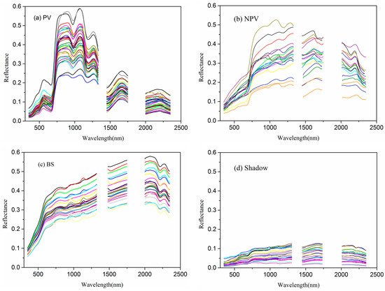
Figure 5.
Spectral library of each endmember class. (a) PV; (b) NPV; (c) bare soil (BS); (d) shadow.
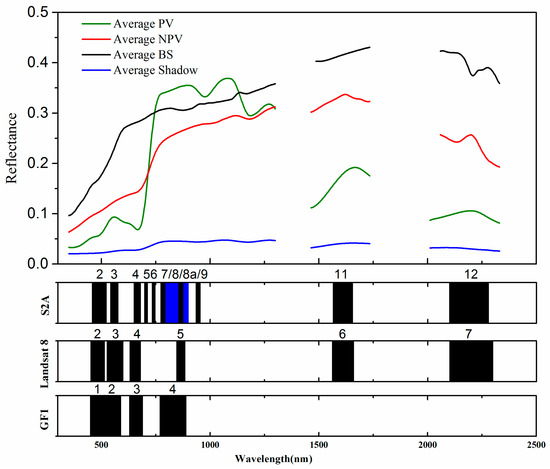
Figure 6.
Average reflectance of selected PV, NPV, BS, and shadow endmembers, and band position of three main sensors.
Figure 5 describes endmember spectra’s spatial changeability. The spectral curve of healthy PV always shows characteristics of “peak and valley”, shown in Figure 5a, the visible domain valley (blue and red at 450 and 670 nm) was mainly caused by the strong absorption of chlorophyll, and they were perceptibly different than the spectral characteristics of PV endmembers in the spectral-domain range of 750–1250 nm. Throughout the entire spectral curve, PV displayed noticeable disparities between red and near-infrared, but NPV and BS did not (Figure 5b,c). Therefore, PV could be distinguished from NPV and BS. There were clear absorption features near shortwave infrared 2100 nm for NPV, mainly due to nonstructural components such as cellulose, hemicellulose, and lignin, but did not have such absorption characteristics for BS and PV. Because there was significantly different chlorophyll content for PV and NPV, PV and NPV could be distinguished according to the red edge position. Due to the influence of NPV type, humidity, and decomposition degree, the reflectance of the VIS–NIR spectral NPV may have been higher or lower than BS. Consequently, it was difficult to make a distinction between NPV and BS. Regardless of difficulty, the spectral characteristic of the NPV in 500–900 nm and around 2100 nm was significantly distinct from BS. A bow-shaped protuberance was shown in the 500–900 nm spectral range for BS [51]. The non-cellulose element of NPV resulted in spectral-absorption features at about 2100 nm [52]. Therefore, according to the unique characteristics of each endmember, endmember spectra within the specific spectral range could effectively distinguish between PV, NPV, and BS. Shadow reflectance was almost nonexistent and consistent throughout the whole spectral curve (Figure 5d), so shadows indicated noticeable variances with the three other endmembers.
According to characteristics of the average PV–NPV–BS–shadow spectral curves (Figure 6) corresponding to bands of the S2, L8, and GF1 satellites, there were three "red edge" bands for the S2 sensor corresponding to bands 4–6, and five more NIR bands than those in the Landsat 8 in the NIR domain. Moreover, bands of S2 MSI were narrower than those corresponding to L8 OLI and GF1 WFV.
4.2. Endmember Combination Optimization
Two scenarios, PV–NPV–BS (3-EM) and PV–NPV–BS–shadow (4-EM), were compared for three sensors to estimate fPV and fNPV. Results (Table 2) showed that model unmixing accuracy based on the 4-EM model was greatly improved compared to that of the 3-EM model, especially when the NSMM was utilized. Accuracy based on 4-EM was higher than that of 3-EM for model unmixing and the cross-validation of each endmember. Spectrally unmixed fPV and fNPV with 4-EM from the S2 sensor had significantly low RMSE with the reference fractions. About 1% to 5% of the unmixing RMSE was caused by the shadow effects with the LSMM, and 1% to 7% of the unmixing RMSE was caused by the shadow effects with the NSMM. In the presence of a shadow endmember, the validation RMSE for all endmembers was evidently reduced, particularly for fNPV, where the RMSE could be reduced by more than 50%, which indicates that the shadow had a severe effect on sparse vegetation coverage estimation when spectral mixture models were employed.
Table 2.
3-EM and 4-EM for unmixing based on three sensors and accuracy of each endmember-coverage estimation for sensors with different spatial resolutions and applied methods. GF1_4B represents bands 1–4; L8_4B represents bands 2–5 (responding to GF1_4B); S2_4B represents bands 2–4 and 8 (responding to GF1_4B and L8_4B) composed with 10 m spatial resolution; S2_6B represents bands 2–4, 8a, 11, and 12 (responding to L8_6B), and S2_11B represents bands 2–9, 8a, 11 and 12 composed with 10 m spatial resolution.
This finding is consistent with Wang et al. [53,54,55], who indicated that shadows significantly influence multiple scattering. Although Hostert et al. reported that using a 3-4 endmember model on an original Landsat TM image does not affect fractional-cover estimates for dense vegetation [56], shadow interference is reduced considerably by treating them as independent endmembers in arid areas with the sparse vegetation. Then, the accuracy of estimated endmember fractions would be significantly improved, especially for areas existing in the notable nonlinear spectral unmixing with 7% accuracy improved and NPV endmember with more than 50% accuracy improved. Above all, shadows are an important variable background factor in arid areas. Their participation for the estimation of fPV and fNPV removes parts of interference factors with SMA for pixel unmixing.
4.3. Comparison between Different Sensors
The unmixing fraction images and validation scatterplots are shown in Figure 7. It can be noted that the precision of S2 was obviously higher than that of L8 and GF1, with more bands and higher spatial resolution, especially for fNPV estimation. The RMSE of fPV estimated by the three sensors was very similar, as was the RMSE of the fBS. However, according to R2 and the scatterplot in Figure 7, we could know that each endmember coverage extracted by the Sentinel-2A sensor was closest to its measured coverage according to the cross-validation, and its coverage of each estimated endmember was the most reliable and had the best correlation, after the Landsat-8 OLI and GF1 WFV sensors.
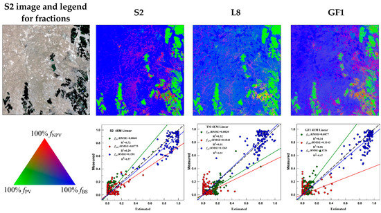
Figure 7.
Endmember fraction maps and scatterplots. Fraction maps estimated by Sentinel-2 with eleven bands and 10 m spatial resolution, Landsat-8 with six bands and 30 m spatial resolution, and GF1 with four bands and 16 m spatial resolution by linear spectral-mixture model (LSMM). Scatterplots illustrate the relation between estimated and reference fractional cover of PV, NPV, and BS estimated by Sentinel-2, Landsat-8, and GF1. Dotted line shows 1:1 agreement; linear fit between measured and estimated value shown by full line. R2 and RMSE are also shown. N = 111 in all circumstances.
4.3.1. Effects of Spatial Resolution
According to the sensor comparison with the four same wavebands, S2 had the lowest error, followed by GF1 and L8, which just responded to a decrease of spatial-resolution of the three sensors. The comparison of S2_6B and L8_6B showed similar results, which proves the importance of spatial resolution for the fPV and fNPV estimation of sparse vegetation in arid regions. The probable cause is that SMA demands spectral knowledge of each type of land surface feature, and their temporal and spatial variation. No matter which method was adopted, error rates increased with the reduction of spatial resolution since the sparse vegetation signals are prone to be covered by the soil background information [57,58,59]. Therefore, high resolution imagery data sets can be used to produce high accuracy fPV and fNPV estimation in comparison to coarse resolution data sets because the increase of vegetation proportion in each scale [60].
4.3.2. Effects of Additional Spectral Bands
With the same spatial resolution, only the four bands, six bands, and eleven bands scenes of the S2 sensor are compared in Table 2. According to the validation accuracy, the S2_4B including VIS-NIR wavebands show the best accuracy for fPV and fBS estimation (RMSEPV = 0.0657, RMSEBS = 0.1190), while S2_6B demonstrated the lowest accuracy for fPV estimation in the case of two SWIR bands than S2_4B, but it is better for fNPV estimation. Although the reflectance in the SWIR spectral region is similar and separable between each endmember, it did not contribute much to improving the accuracy of fPV and fNPV estimation with S2 sensor. This conclusion is different from Asner’s research to extract litter, green canopy and soil from the SWIR-2 (2100–2400 nm) region [8]. However, the accuracy of S2_11B with two more NIR bands (one of which is NIR narrow band) and three RE bands than S2_6B was obviously improved for fNPV estimation. In the study, we noticed that the VIS wavebands were significant for fPV estimation, and more RE and NIR wavebands were important to improve the accuracy of NPV fractional estimation. The above conclusions were consistent with the characteristics of the PV-NPV-BS-Shadow average spectral curves (Figure 5 and Figure 6) in that they were obviously different in the RE and NIR spectral range.
It is well-known that the red band and the red edge region are the sensitive spectral range for chlorophyll detection, and a series of bands in the red edge region with the sensors will greatly improve the monitoring of green vegetation in arid areas [58,61]. Otherwise, Li et al. have concluded that the red edge bands were better than the SWIR bands for monitoring NPV based on Landsat 8 OLI and Sentinel-2A MSI [62,63], which are consistent with our results. Except for finer spatial resolution and red edge bands, the narrower bandwidth of S2 compared to L8 and GF1 could be attributed to better performance in fPV and fNPV estimation, since narrow bands are more sensitive to changes in vegetation characteristics [61], and could diminish the impact of a bare-soil background when vegetation cover is sparse [55,64].
4.4. Effects of Nonlinear Mixture Process
Comparing NSMM with LSMM in Table 2 and Figure 8, it could be seen that the complicated nonlinear model could not acquire better results, which means that the nonlinear multiscatter process between the four endmembers was not obvious at the 10–30 m spatial scale. It is well-known that the multiscatter process is common for single desert vegetation [22,51], but could be eliminated at coarse spatial resolution (10–30 m) since desert vegetation is small and sparse [17,65,66]. In the study, the nonlinear mixture for NSMM is not obvious, there are two possible reasons:
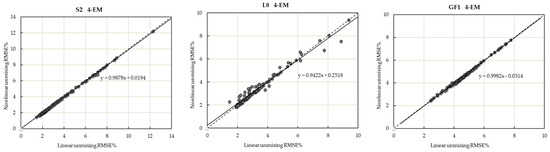
Figure 8.
Unmixing relative RMSE relationship between NSMM and LSMM. N = 111 in all circumstances.
(i) First, the canopy endmember spectra were used (including the inner multiple scattering in the canopy). Although we set the black cloth under the PV and NPV endmember canopies and shortened the distance between the top of the plants and the ASD probe, but the endmember spectra are not absolutely pure, and the multiple scattering effects of radiometric interactions within sparse and low canopies could not be eliminated. In our previous research, we learned that there was indeed a nonlinear spectral mixing effect between photosynthetic/non-photosynthetic vegetation and bare soil with the individual vegetation, the intensity of which depends on the three-dimensional structure (planophile or erectophile) of the vegetation canopy. Especially, the nonlinear spectral mixture effects were obvious for the erectophile vegetation type [51]. Thus, the canopy endmember spectra contained the nonlinear process.
(ii) Second, there are the other factors or big noise disturbing PV-NPV-BS separation in a pixel. Because NSMM was more sensitive to noise, the accuracy of NSMM dropped with increasing noise levels [53], even up to a point that LSMM performed better than NSMM for many cases [58,67]. Then, virtual-endmember-based NSMM and formed by the interactive term generally suffers more from collinearity issues compared with LSMM. The degree of collinearity increases with increasing noise, and the collinearity has contributed a large part to the error [67]. In the paper, shadows are an important variable background noise factor in arid areas in the 3-EM models, so that NSMM in the 3-EM model obviously did not perform as well as LSMM. However, unpredictable noise for sparse vegetation is still unavoidable and leads to the existence of collinearity problems, which cannot achieve the good performance of NSMM in the 4-EM model.
Although the multiple scattering is obvious on the scale of individual vegetation in our previous research [51], but as the spatial scale increases, the nonlinear multiscatter process was not obvious for PV and NPV fractional cover estimation at the 10–30 m spatial scale in the arid area. Therefore, there are limitations to using NSMM with large-scale data in arid regions.
5. Conclusions
On the basis of field spectra, and airborne and satellite data, we analyzed the performance of the new Sentinel-2 MSI, Landsat8 OLI, and GF1 WFV sensors for the estimation of PV, NPV, and BS fractions in arid regions by the LSMM and NSMM. Our conclusions are summarized as follows: first, the Sentinel-2 sensor, with more red edge bands and higher spatial resolution, could improve accuracy to achieve fPV and fNPV in arid regions when compared to L8 and GF1; second, more red edge and NIR bands of S2 could greatly improve fNPV estimation accuracy, a key obstacle for retrieving fNPV on the basis of multispectral satellite data; third, with the same four or six bands, S2 performed better than L8 and GF1, and GF1 performed better than L8; they were mainly determined by spatial resolution. Therefore, high spatial resolution is very important for retrieving fPV and fNPV in arid regions when multispectral satellite data are utilized. Finally, shadow endmembers are inevitable in arid regions for satellite-based unmixing, and nonlinear mixture effects were not obvious at the 10–30 m spatial-resolution scale. Throughout the study, it was greatly helpful to improve the performance of main medium-spatial-resolution sensors in vegetation-coverage estimation.
Author Contributions
Conceptualization, C.J. and X.L.; methodology, C.J. and X.L.; software, C.J.; validation, X.L.; formal analysis, H.W. and S.L.; investigation, H.W.; resources, H.W.; data curation, H.W.; writing—original-draft preparation, C.J.; writing—review and editing, C.J., X.L. and S.L.; visualization, H.W. and S.L.; supervision, X.L.; project administration, X.L.; funding acquisition, X.L. All authors have read and agreed to the published version of the manuscript.
Acknowledgments
This work was supported by the National Key Research and Development Program (grant No. 2016YFC0500806); GF6 Project (grant No. 30-Y20A03-9003-17/18); the National Natural Science Foundation of China (grant No. 41571421); the National Natural Science Foundation of China (grant No. 31360204); and Science and Technology Research Project of Chongqing Education Commission (grant No. KJ1600530).
Conflicts of Interest
The authors declare no conflict of interest.
References
- Guerschman, J.P.; Hill, M.J.; Renzullo, L.J.; Barrett, D.J.; Marks, A.S.; Botha, E.J. Estimating fractional cover of photosynthetic vegetation, non-photosynthetic vegetation and bare soil in the Australian tropical savanna region upscaling the EO-1 Hyperion and MODIS sensors. Remote Sens. Environ. 2009, 113, 928–945. [Google Scholar] [CrossRef]
- Li, X.S.; Zheng, G.X.; Wang, J.Y.; Ji, C.C.; Sun, B.; Gao, Z.H. Comparison of Methods for Estimating Fractional Cover of Photosynthetic and Non-Photosynthetic Vegetation in the Otindag Sandy Land Using GF-1 Wide-Field View Data. Remote Sens. 2016, 8, 800. [Google Scholar] [CrossRef]
- Reynolds, J.F.; Smith, D.M.S.; Lambin, E.F.; Turner, B.; Mortimore, M.; Batterbury, S.P.; Downing, T.E.; Dowlatabadi, H.; Fernández, R.J.; Herrick, J.E.; et al. Global desertification: Building a science for dryland development. Science 2007, 316, 847–851. [Google Scholar] [CrossRef] [PubMed]
- Tucker, C.J. Red and photographic infrared linear combinations for monitoring vegetation. Remote Sens. Environ. 1979, 8, 127–150. [Google Scholar] [CrossRef]
- Chen, X.; Vierling, L. Spectral mixture analyses of hyperspectral data acquired using a tethered balloon. Remote Sens. Environ. 2006, 103, 338–350. [Google Scholar] [CrossRef]
- Zhao, D.H.; Li, J.L.; Qi, J.G. Identification of red and NIR spectral regions and vegetative indices for discrimination of cotton nitrogen stress and growth stage. Comput. Electron. Agric. 2005, 48, 155–169. [Google Scholar] [CrossRef]
- Okin, G.S. Relative spectral mixture analysis—A multitemporal index of total vegetation cover. Remote Sens. Environ. 2007, 106, 467–479. [Google Scholar] [CrossRef]
- Asner, G.P.; Lobell, D.B. A Biogeophysical Approach for Automated SWIR Unmixing of Soils and Vegetation. Remote Sens. Environ. 2000, 74, 99–112. [Google Scholar] [CrossRef]
- Daughtry, C.S.T.; McMurtrey, J.E.; Chappelle, E.W.; Dulaney, W.P.; Irons, J.R.; Satterwhite, M.B. Potential for Discriminating Crop Residues from Soil by Reflectance and Fluorescence. Agron. J. 1995, 87, 165–171. [Google Scholar] [CrossRef]
- Galvão, L.S.; Ícaro, V.; Filho, R.A. Effects of Band Positioning and Bandwidth on NDVI Measurements of Tropical Savannas. Remote Sens. Environ. 1999, 67, 181–193. [Google Scholar] [CrossRef]
- Garrigues, S.; Allard, D.; Baret, F.; Weiss, M. Influence of landscape spatial heterogeneity on the non-linear estimation of leaf area index from moderate spatial resolution remote sensing data. Remote Sens. Environ. 2006, 105, 286–298. [Google Scholar] [CrossRef]
- Lehnert, L.; Meyer, H.; Thies, B.; Reudenbach, C.; Bendix, J. Monitoring plant cover on the Tibetan Plateau: A multi-scale remote sensing based approach. In Proceedings of the Egu General Assembly Conference, Vienna, Austria, 27 April–2 May 2014. [Google Scholar]
- Teillet, P.M.; Staenz, K.; William, D.J. Effects of spectral, spatial; radiometric characteristics on remote sensing vegetation indices of forested regions. Remote Sens. Environ. 1997, 61, 139–149. [Google Scholar] [CrossRef]
- Clasen, A.; Somers, B.; Pipkins, K.; Tits, L.; Segl, K.; Brell, M.; Kleinschmit, B.; Spengler, D.; Lausch, A.; Förster, M. Spectral Unmixing of Forest Crown Components at Close Range, Airborne and Simulated Sentinel-2 and EnMAP Spectral Imaging Scale. Remote Sens. 2015, 7, 15361–15387. [Google Scholar] [CrossRef]
- Yang, J.; Weisberg, P.J.; Bristow, N.A. Landsat remote sensing approaches for monitoring long-term tree cover dynamics in semi-arid woodlands: Comparison of vegetation indices and spectral mixture analysis. Remote Sens. Environ. 2012, 119, 62–71. [Google Scholar] [CrossRef]
- Asner, G.P.; Heidebrecht, K.B. Spectral unmixing of vegetation, soil and dry carbon cover in arid regions: Comparing multispectral and hyperspectral observations. Int. J. Remote Sens. 2002, 23, 3939–3958. [Google Scholar] [CrossRef]
- Guerschman, J.P.; Scarth, P.F.; Mcvicar, T.R.; Renzullo, L.J.; Malthus, T.J.; Stewart, J.B.; Rickards, J.E.; Trevithick, R. Assessing the effects of site heterogeneity and soil properties when unmixing photosynthetic vegetation, non-photosynthetic vegetation and bare soil fractions from Landsat and MODIS data. Remote Sens. Environ. 2015, 161, 12–26. [Google Scholar] [CrossRef]
- Okin, G.S.; Clarke, K.D.; Lewis, M.M. Comparison of methods for estimation of absolute vegetation and soil fractional cover using MODIS normalized BRDF-adjusted reflectance data. Remote Sens. Environ. 2013, 130, 266–279. [Google Scholar] [CrossRef]
- Boardman, J.W. Automated spectral unmixing of AVIRIS data using convex geometry concepts. Summ. Annu. JPL Airborne Geosci. Workshop 1993, 1, 11–14. [Google Scholar]
- Keshava, N.; Mustard, J.F. Spectral unmixing. IEEE Signal Process. Mag. 2002, 19, 44–57. [Google Scholar] [CrossRef]
- Borel, C.C.; Gerstl, S.A.W.; Borel, C.C.; Gerstl, S.A.W. Nonlinear spectral mixing models for vegetative and soil surfaces. Remote Sens. Environ. 1994, 47, 403–416. [Google Scholar] [CrossRef]
- Ray, T.W.; Murray, B.C. Nonlinear spectral mixing in desert vegetation. Remote Sens. Environ. 1996, 55, 59–64. [Google Scholar] [CrossRef]
- Roberts, D.A.; Smith, M.O.; Adams, J.B. Green vegetation, nonphotosynthetic vegetation, and soils in AVIRIS data. Remote Sens. Environ. 1993, 44, 255–269. [Google Scholar] [CrossRef]
- Marshall, M.; Thenkabail, P. Advantage of hyperspectral EO-1 Hyperion over multispectral IKONOS, GeoEye-1, WorldView-2, Landsat ETM+, and MODIS vegetation indices in crop biomass estimation. ISPRS J. Photogramm. Remote Sens. 2015, 108, 205–218. [Google Scholar] [CrossRef]
- Wang, W.; Duan, Z. Gansu Yearbook; Chinese Literature Press: Beijing, China, 2017; Volume 308. [Google Scholar]
- Muir, J.; Schmidt, M.; Tindall, D.; Trevithick, R.; Scarth, P.; Stewart, J.B. Field Measurement of Fractional Ground Cover: A Technical Handbook Supporting Ground Cover Monitoring for Australia; Australian Bureau of Agricultural and Resource Economics and Sciences: Canberra, Australia, 2011.
- Adams, J.B.; Smith, M.O.; Gillespie, A.R. Imaging spectroscopy: Interpretation based on spectral mixture analysis. In Remote Geochem. Anal. Top. Remote Sens; Pieters, C.M., Englert, P.A.J., Eds.; Cambridge University Press: New York, NY, USA, 1993; pp. 145–166. [Google Scholar]
- Drake, J.J.; Settle, N.A. Linear Mixing and the Estimation of Ground Cover Proportions. Int. J. Remote Sens. 1993, 14, 1159–1177. [Google Scholar]
- Adams, J.B.; Smith, M.O.; Johnson, P.E. Spectral mixture modeling: A new analysis of rock and soil types at the Viking Lander I site. J. Geophys. Res. Atmos. 1986, 91, 8098–8112. [Google Scholar] [CrossRef]
- Gillespie, A.R.; Smith, M.O.; Adams, J.B.; Willis, S.C.; Fischer, A.F.; Sabol, D.E. Interpretation of Residual Images: Spectral Mixture Analysis of AVIRIS Images. In Proceedings of the 2nd AVIRIS Workshop, Owens Valley, Pasadena, CA, USA, 4–5 June 1990; pp. 243–270. [Google Scholar]
- Theseira, M.A.; Thomas, G.; Sannier, C.A.D. An evaluation of spectral mixture modelling applied to a semi-arid environment. Int. J. Remote Sens. 2002, 23, 687–700. [Google Scholar] [CrossRef]
- Vikhamar, D.; Solberg, R. Snow-cover mapping in forests by constrained linear spectral unmixing of MODIS data. Remote Sens. Environ. 2003, 88, 309–323. [Google Scholar] [CrossRef]
- Wu, C.; Murray, A.T. Estimating impervious surface distribution by spectral mixture analysis. Remote Sens. Environ. 2003, 84, 493–505. [Google Scholar] [CrossRef]
- Zhang, L.; Wu, B.; Huang, B.; Li, P. Nonlinear estimation of subpixel proportion via kernel least square regression. Int. J. Remote Sens. 2007, 28, 4157–4172. [Google Scholar] [CrossRef]
- Chang, C.I.; Heinz, D.C. Constrained subpixel target detection for remotely sensed imagery. IEEE Trans. Geosci. Remote Sens. 2000, 38, 1144–1159. [Google Scholar] [CrossRef]
- Heinz, D.C.; Chang, C.I. Fully constrained least squares linear spectral mixture analysis method for material quantification in hyperspectral imagery. IEEE Trans. Geosci. Remote Sens. 2001, 39, 529–545. [Google Scholar] [CrossRef]
- Bioucas-Dias, J.M.; Plaza, A.; Dobigeon, N.; Parente, M.; Du, Q.; Gader, P.; Chanussot, J. Hyperspectral Unmixing Overview: Geometrical, Statistical, and Sparse Regression-Based Approaches. Sel. Top. Appl. Earth Obs. Remote Sens. IEEE J. 2012, 5, 354–379. [Google Scholar] [CrossRef]
- Chen, J.; Richard, C.; Honeine, P. Nonlinear Unmixing of Hyperspectral Data Based on a Linear-Mixture/Nonlinear-Fluctuation Model. Signal Process. IEEE Trans. 2013, 61, 480–492. [Google Scholar] [CrossRef]
- Li, X.R.; Cui, J.T.; Zhao, L.Y. Blind nonlinear hyperspectral unmixing based on constrained kernel nonnegative matrix factorization. Signal Image Video Process. 2014, 8, 1555–1567. [Google Scholar] [CrossRef]
- Li, X.R.; Wu, X.M.; Zhao, L.Y. Unsupervised nonlinear decomposing method of hyperspectral imagery. J. Zhejiang Univ. 2011, 45, 607–613. [Google Scholar]
- Camps-Valls, G.; Bruzzone, L. Kernel-based methods for hyperspectral image classification. IEEE Trans. Geosci. Remote Sens. 2005, 43, 1351–1362. [Google Scholar] [CrossRef]
- Mercer, J. Functions of Positive and Negative Type, and their Connection with the Theory of Integral Equations. Philos. Trans. R. Soc. Lond. 1909, 209, 415–446. [Google Scholar] [CrossRef]
- Zaanen, A.C. Linear Analysis; Bibliotheca Mathematica, North-Holland Publishing Co.: Amsterdam, The Netherlands, 1956. [Google Scholar]
- Bhatia, R. Positive Definite Matrices; Princeton University Press: Princeton, NJ, USA, 2015; pp. 259–264. [Google Scholar]
- Ammanouil, R.; Ferrari, A.; Richard, C.; Mathieu, S. Nonlinear unmixing of hyperspectral data with vector-valued kernel functions. IEEE Trans. Image Process. 2017, 26, 340–354. [Google Scholar] [CrossRef]
- Chapelle, O.; Vapnik, V.; Bousquet, O.; Mukherjee, S. Choosing Multiple Parameters for Support Vector Machines. Mach. Learn. 2002, 46, 131–159. [Google Scholar] [CrossRef]
- Broadwater, J.; Chellappa, R.; Banerjee, A.; Burlina, P. Kernel fully constrained least squares abundance estimates. In Proceedings of the 2007 IEEE Geoscience and Remote Sensing Symposium, Barcelona, Spain, 23–28 July 2007. [Google Scholar]
- Camps-Valls, G.; Bruzzone, L. Kernel Methods for Remote Sensing Data Analysis; Wiley: Hoboken, NJ, USA, 2009; pp. 437–451. [Google Scholar]
- Liu, K.H.; Lin, Y.Y.; Chen, C.S. Linear Spectral Mixture Analysis via Multiple-Kernel Learning for Hyperspectral Image Classification. IEEE Trans. Geosci. Remote Sens. 2014, 53, 2254–2269. [Google Scholar] [CrossRef]
- Fan, W.; Hu, B.; Miller, J.; Li, M. Comparative study between a new nonlinear model and common linear model for analysing laboratory simulated-forest hyperspectral data. Int. J. Remote Sens. 2009, 30, 2951–2962. [Google Scholar] [CrossRef]
- Ji, C.; Jia, Y.; Gao, Z.; Wei, H.; Li, X. Nonlinear spectral mixture effects for photosynthetic/non-photosynthetic vegetation cover estimates of typical desert vegetation in western China. PLoS ONE 2017, 12, e0189292. [Google Scholar] [CrossRef] [PubMed]
- Li, T.; Li, X.S.; Li, F. Estimating fractional cover of photosynthetic vegetation and non-photosynthetic vegetation in the Xilingol steppe region with EO-1 hyperion data. Acta Ecol. Sin. 2015, 35, 3643–3652. [Google Scholar]
- Wang, J.; Cao, X.; Chen, J.; Jia, X. Assessment of Multiple Scattering in the Reflectance of Semiarid Shrublands. IEEE Trans. Geosci. Remote Sens. 2015, 53, 4910–4921. [Google Scholar] [CrossRef]
- Fitzgerald, G.J. Shadow fraction in spectral mixture analysis of a cotton canopy. Remote Sens. Model. Ecosyst. Sustain. 2004, 5544, 20–34. [Google Scholar]
- Fitzgerald, G.J.; Pinter, P.J.; Hunsaker, D.J.; Clarke, T.R. Multiple shadow fractions in spectral mixture analysis of a cotton canopy. Remote Sens. Environ. 2005, 97, 526–539. [Google Scholar] [CrossRef]
- Hostert, P.; Röder, A.; Hill, J. Coupling spectral unmixing and trend analysis for monitoring of long-term vegetation dynamics in Mediterranean rangelands. Remote Sens. Environ. 2003, 87, 183–197. [Google Scholar] [CrossRef]
- Gessner, U.; Machwitz, M.; Conrad, C.; Dech, S. Estimating the fractional cover of growth forms and bare surface in savannas. A multi-resolution approach based on regression tree ensembles. Remote Sens. Environ. 2013, 129, 90–102. [Google Scholar] [CrossRef]
- Hansen, M.C.; Defries, R.S.; Townshend, J.R.G.; Sohlberg, R.; Dimiceli, C.; Carroll, M. Towards an operational MODIS continuous field of percent tree cover algorithm: Examples using AVHRR and MODIS data. Remote Sens. Environ. 2002, 83, 303–319. [Google Scholar] [CrossRef]
- Hansen, M.C.; Defries, R.S.; Townshend, J.R.G.; Marufu, L.; Sohlberg, R. Development of a MODIS tree cover validation data set for Western Province, Zambia. Remote Sens. Environ. 2002, 83, 320–335. [Google Scholar] [CrossRef]
- Frank, T.D.; Tweddale, S.A. The effect of spatial resolution on measurement of vegetation cover in three Mojave Desert shrub communities. J. Arid Environ. 2006, 67, 88–99. [Google Scholar] [CrossRef]
- Elvidge, C.D.; Chen, Z. Comparison of broad-band and narrow-band red and near-infrared vegetation indices. Remote Sens. Environ. 1995, 54, 38–48. [Google Scholar] [CrossRef]
- Li, Z.; Guo, X. Non-photosynthetic vegetation biomass estimation in semiarid Canadian mixed grasslands using ground hyperspectral data, Landsat 8 OLI, and Sentinel-2 images. Int. J. Remote Sens. 2018, 39, 6893–6913. [Google Scholar] [CrossRef]
- Zarco-Tejada, P.J.; Hornero, A.; Beck, P.S.A.; Kattenborn, T.; Kempeneers, P.; Hernández-Clemente, R. Chlorophyll content estimation in an open-canopy conifer forest with Sentinel-2A and hyperspectral imagery in the context of forest decline. Remote Sens. Environ. 2019, 223, 320–335. [Google Scholar] [CrossRef]
- Thenkabail, P.S.; Smith, R.B.; Pauw, E.D. Hyperspectral vegetation indices and their relationships with agricultural crop characteristics. Remote Sens. Environ. 2000, 71, 158–182. [Google Scholar] [CrossRef]
- Zheng, G.X.; Li, X.S.; Zhang, G.X.; Wang, J.Y. Spectral mixing mechanism analysis of photosynthetic/non-photosynthetic vegetation and bared soil mixture in the Hunshandake (Otindag) sandy land. Spectrosc. Spectr. Anal. 2016, 36, 1063–1068. [Google Scholar]
- Lehnert, L.W.; Meyer, H.; Wang, Y.; Miehe, G.; Thies, B.; Reudenbach, C.; Bendix, J. Retrieval of grassland plant coverage on the Tibetan Plateau based on a multi-scale, multi-sensor and multi-method approach. Remote Sens. Environ. 2015, 164, 197–207. [Google Scholar] [CrossRef]
- Chen, X.; Chen, J.; Jia, X.; Somers, B.; Wu, J.; Coppin, P. A Quantitative Analysis of Virtual Endmembers’ Increased Impact on the Collinearity Effect in Spectral Unmixing. IEEE Trans. Geosci. Remote Sens. 2011, 49, 2945–2956. [Google Scholar] [CrossRef]
© 2020 by the authors. Licensee MDPI, Basel, Switzerland. This article is an open access article distributed under the terms and conditions of the Creative Commons Attribution (CC BY) license (http://creativecommons.org/licenses/by/4.0/).