Detecting Land Degradation in Eastern China Grasslands with Time Series Segmentation and Residual Trend analysis (TSS-RESTREND) and GIMMS NDVI3g Data

 ,
,  ,
,
Abstract

1. Introduction
2. Materials and Methods
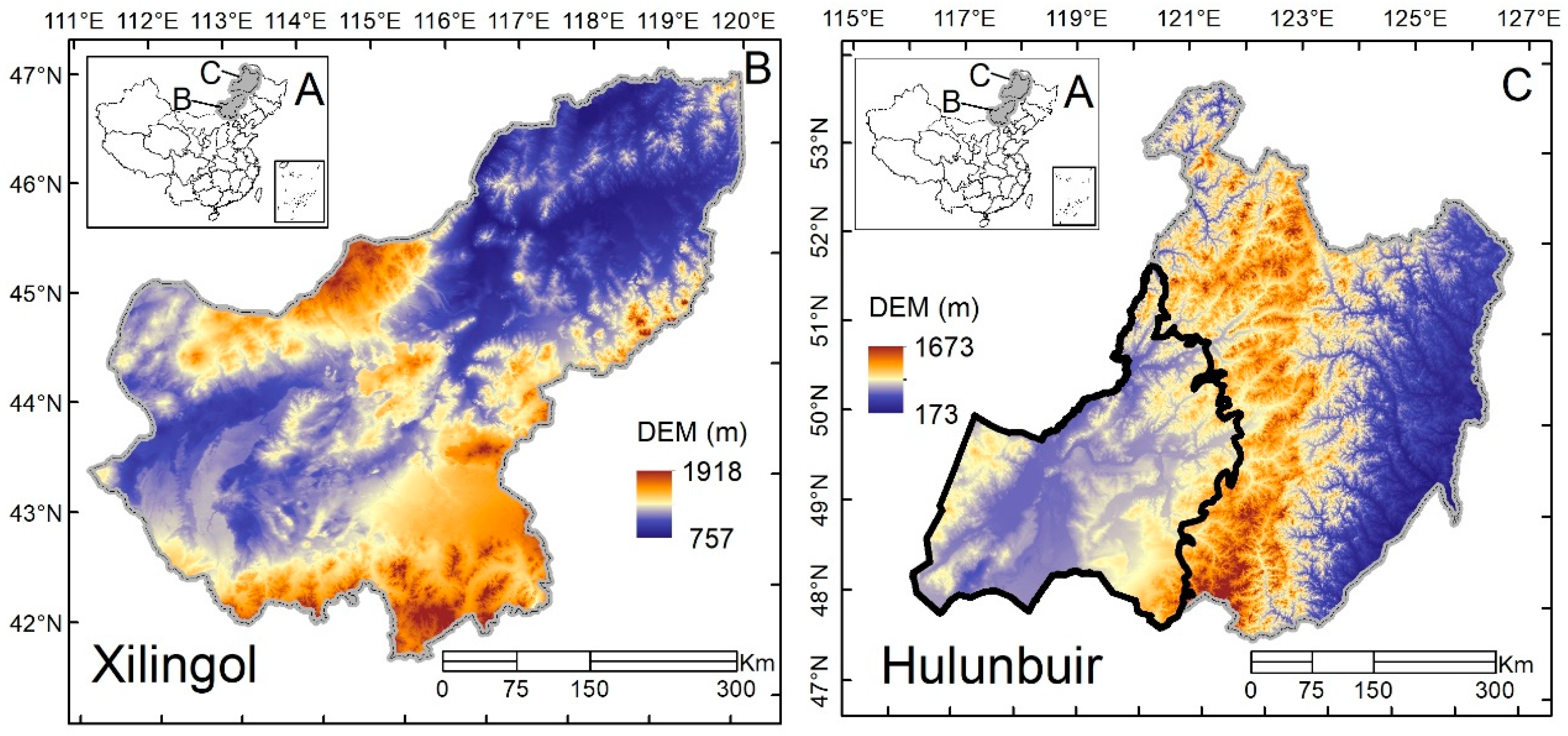
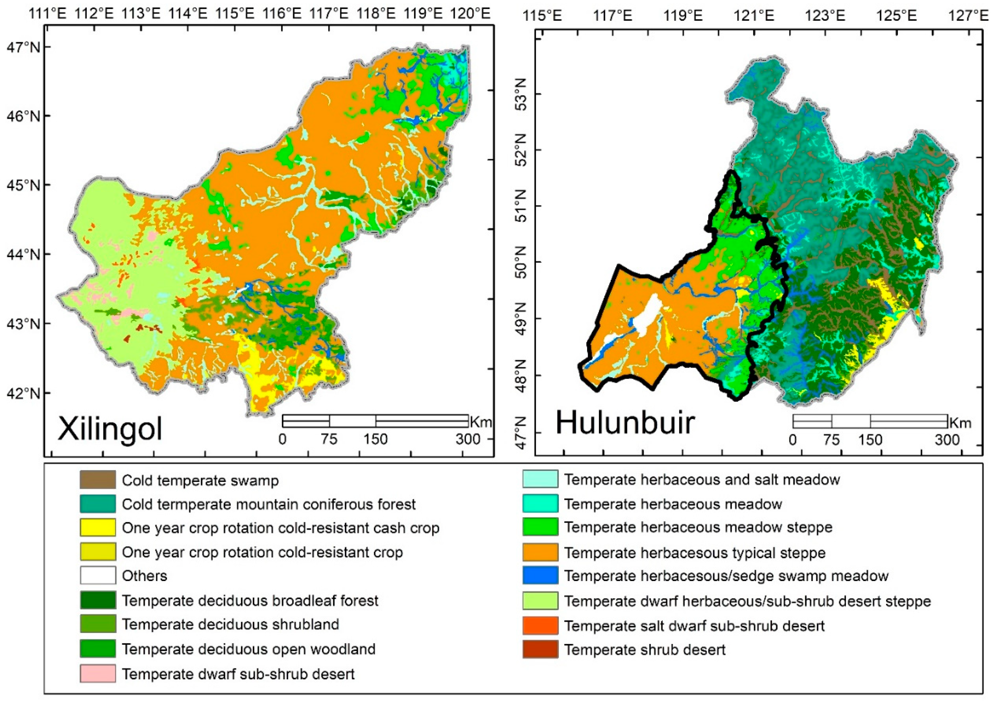
2.1. Study Area
2.2. Data Source and Pre-Processing
2.2.1. GIMMS NDVI3g Data
2.2.2. Meteorological Dataset
2.2.3. Vegetation Types
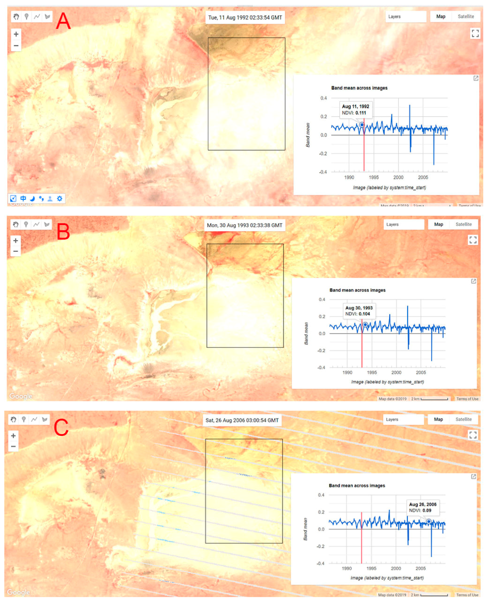
2.2.4. Validating Breakpoint Timing in Google Earth Engine
2.3. Methods
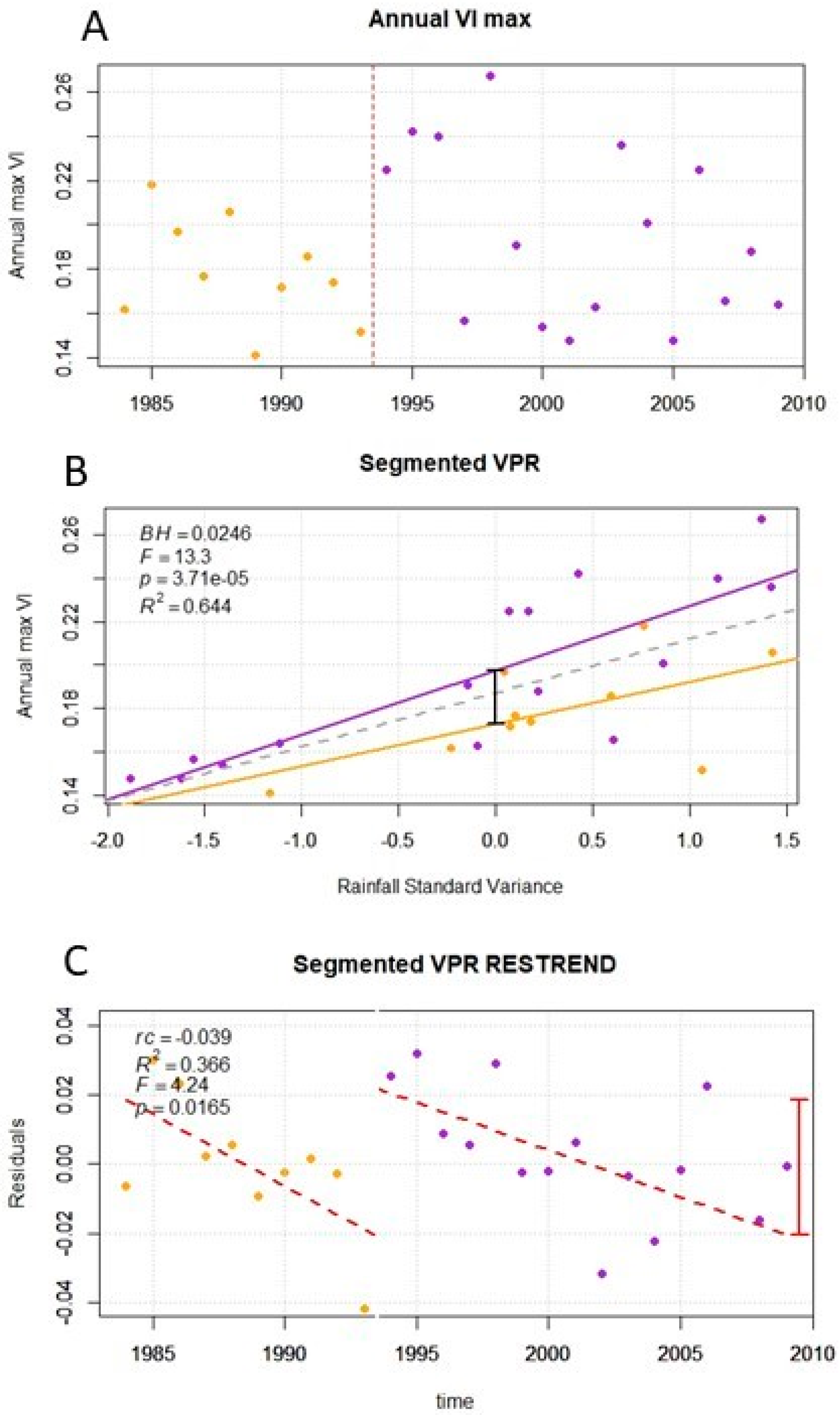
2.3.1. RESTREND
- The VPR is significant and positive (slope > 0). Recommended values for significance are R2 > 0.3 at p < 0.05 significance level.
- A residual trend is gradual and consistent or at least monotonic for the entire time series [41].
- The VPR must remain consistent with time, which is defined as a VPR that is comparable throughout the entire time series, i.e., no major structural changes occurring within the ecosystem [7].
2.3.2. TSS-RESTREND
- If a pixel has a significant VPR (α = 0.05) and no significant breakpoints in the VPR-residuals (α = 0.05), it meets all the criteria for a standard RESTREND.
- If a significant breakpoint is detected in the VPR-Residuals, a Chow test is also applied to the VPR. For a pixel with a significant breakpoint in the VPR-Residuals (α = 0.05) but not in the VPR (α = 0.05), a segmented RESTREND is applied, as shown in Burrell et al. [8], in which a multivariate regression between the VPR-Residuals, time and a dummy variable that is 0 before the breakpoint and 1 after it:where x = years, z = value of the dummy variable (0 or 1). β0 is intercept, β1 is slope, β2 is the offset at the breakpoint and β3 = the change in the slope at the breakpoint.yi = β0 + β1xi + β2zi+ β3xizi
- If a pixel has a significant breakpoint in VPR, it may indicate a significant structural change to the ecosystem during the study period [46]. Therefore, it is not valid to assume that the optimal duration of precipitation is equivalent to either side of the breakpoint. Thus, the time series NDVImax is separated and a new VPR is recalculated separately on either side of the breakpoint. In order to make it possible to compare with different accumulation and offset periods across the breakpoint, Burrell et al. [8] converted the optimal precipitation into a standard score:where z = standard score, xi = observed values, μ = mean of that accumulation period for the entire time series, σ = standard deviation. Then a multivariate regression is fitted to the time series standard scores:where x = the standardized precipitation in formula (3) for year i, z = value of the dummy variable (0 or 1), β0 is intercept, β1 is slope, β2 is the offset at the breakpoint and β3 is the change in the slope at the breakpoint.yi = β0 + β1xi + β2zi+ β3xizi i = 1984, …, 2009The total change of a pixel with a segmented VPR is calculated by adding the residual change to the VPR break height (β2). The residual change is calculated with segmented RESTREND.
- Pixels, where no significant model can be fitted, are classified as indeterminate.
2.3.3. Linear Trend Analysis (LTA)
2.3.4. Comparison RESTREND, TSS-RESTREND, and LTA Results
3. Results
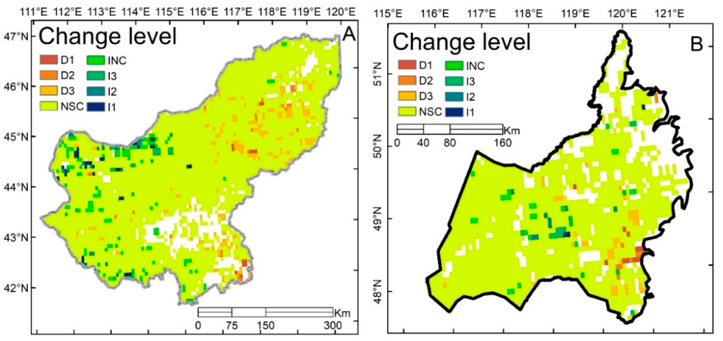
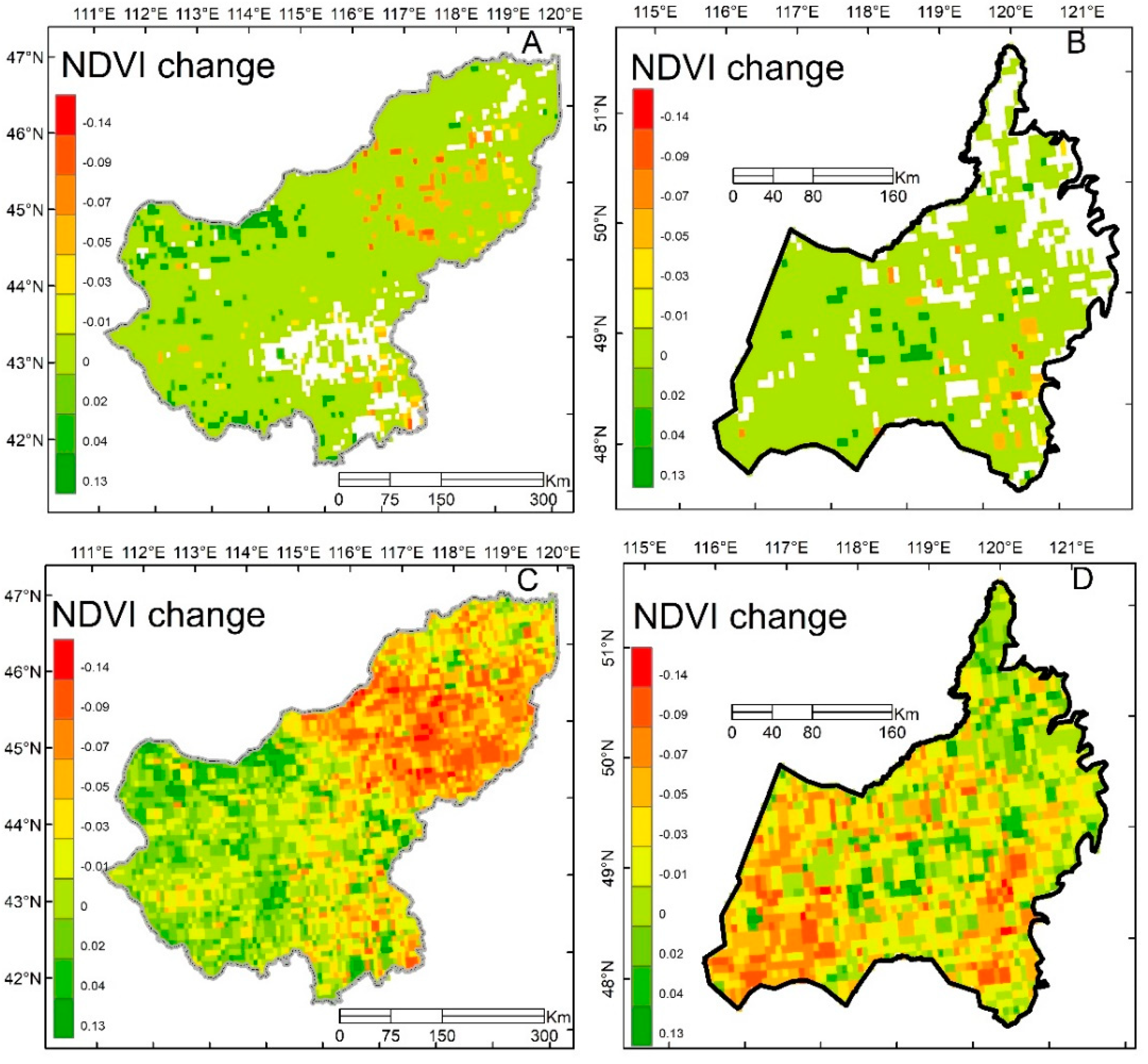
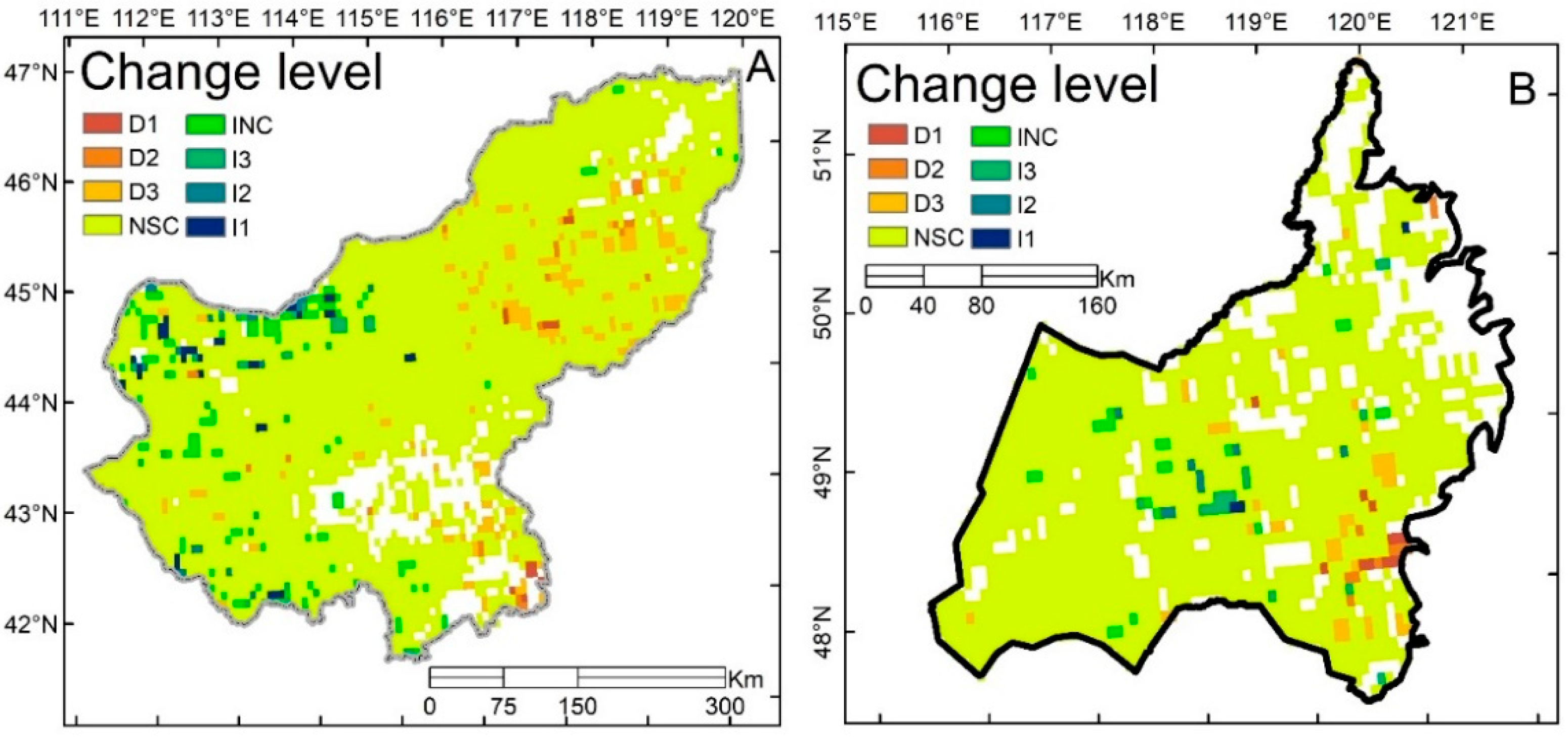
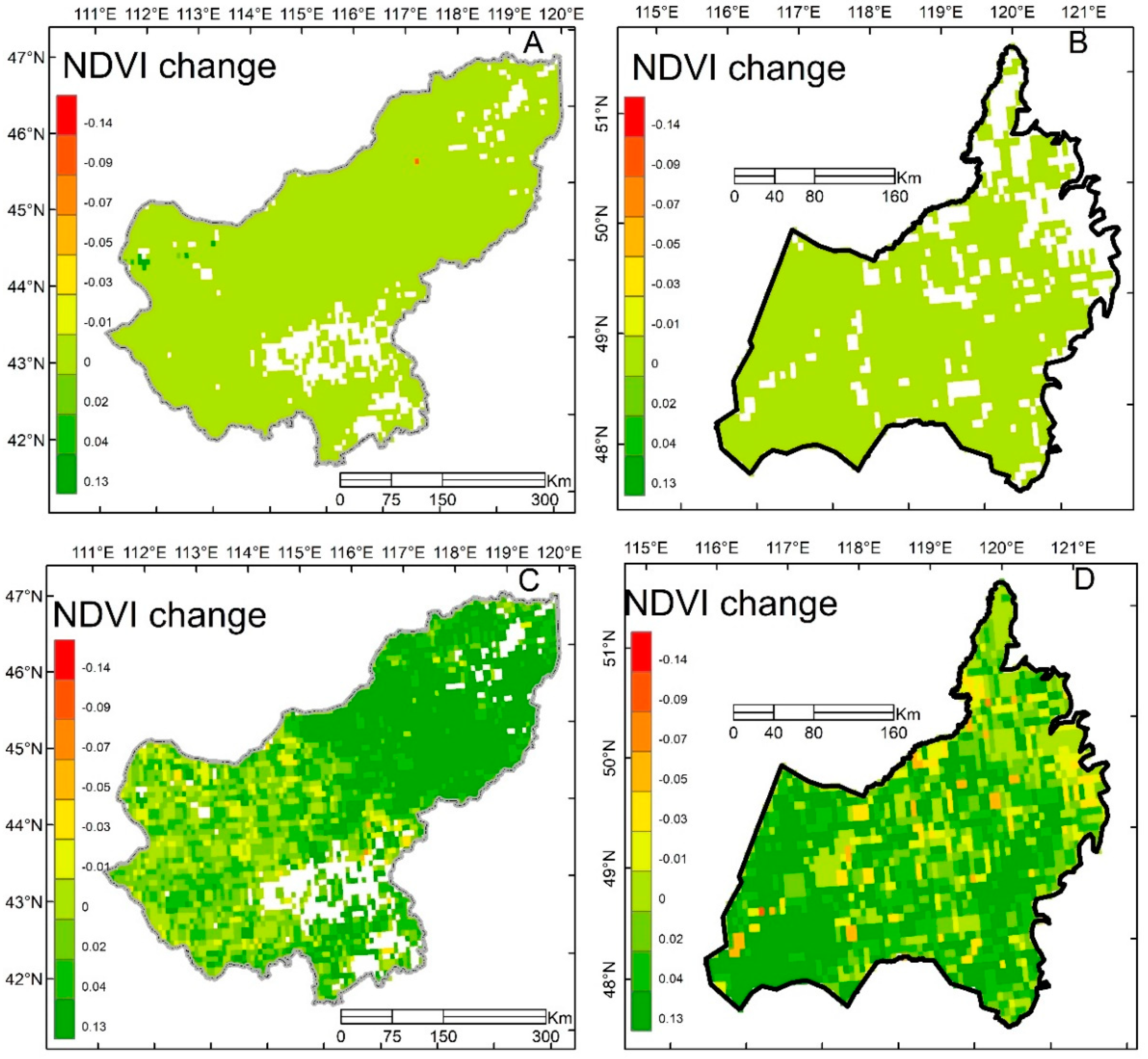
3.1. Vegetation Change Detection by TSS-RESTREND, RESTREND, and LTA
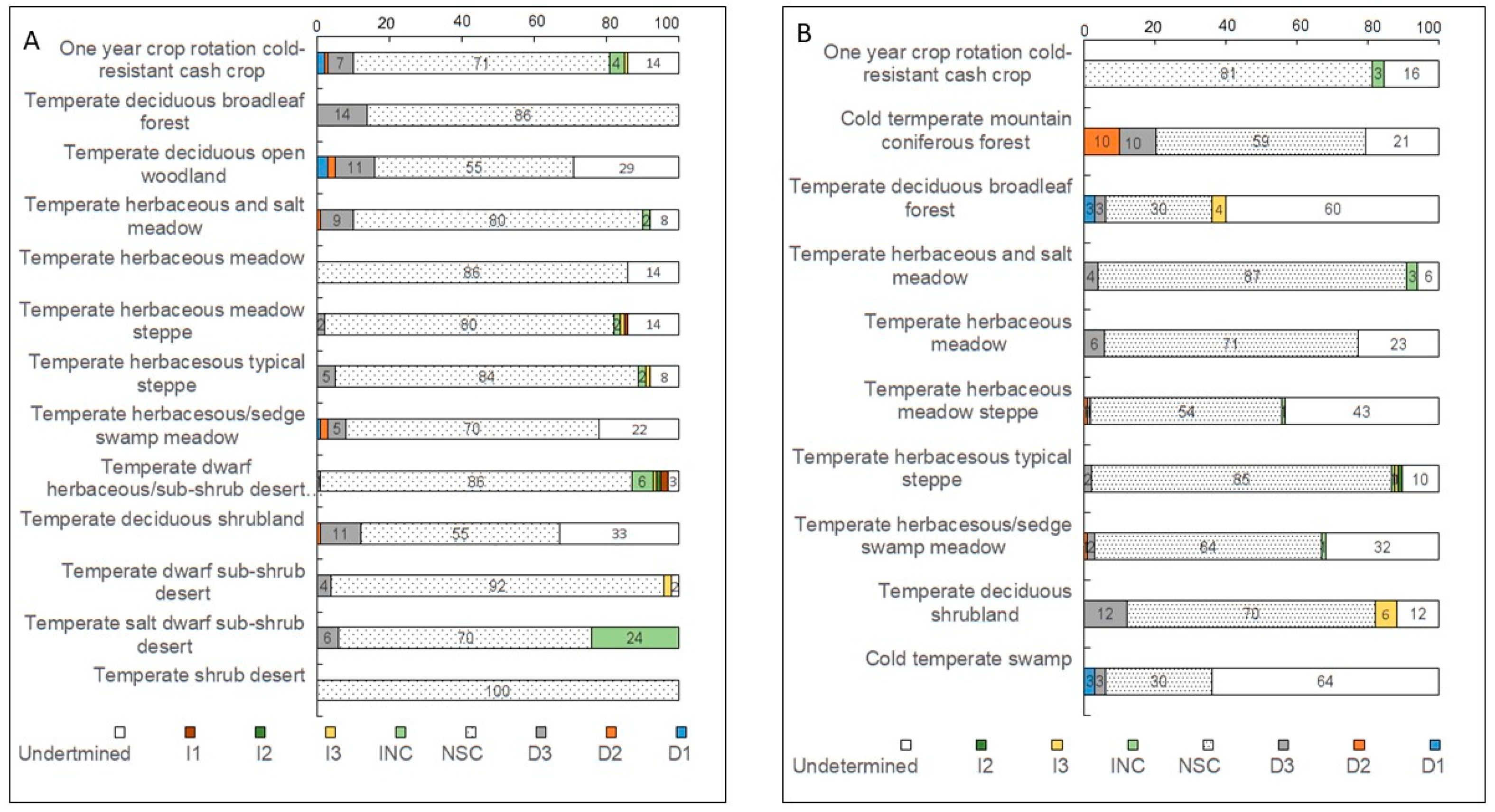
3.2. Trend and Breakpoint Analyses with TSS-RESTREND
3.3. Method Comparison
4. Discussion
4.1. Performance of TSS-RESTREND, RESTREND, and LTA
4.2. Validity of Breakpoint Detection
4.3. Land Degradation
5. Conclusions
Author Contributions
Funding
Acknowledgments
Conflicts of Interest
References
- Hao, L.; Sun, G.; Liu, Y.; Gao, Z.; He, J.; Shi, T.; Wu, B. Effects of precipitation on grassland ecosystem restoration under grazing exclusion in Inner Mongolia, China. Landsc. Ecol. 2014, 29, 1657–1673. [Google Scholar] [CrossRef]
- Qi, J.; Chen, J.; Wan, S.; Ai, L. Understanding the coupled natural and human systems in Dryland East Asia. Environ. Res. Lett. 2012, 7, 015202. [Google Scholar] [CrossRef]
- Ruppert, J.C.; Harmoney, K.; Henkin, Z.; Snyman, H.A.; Sternberg, M.; Willms, W.; Linstädter, A. Quantifying drylands’ drought resistance and recovery: The importance of drought intensity, dominant life history and grazing regime. Glob. Chang. Biol. 2015, 21, 1258–1270. [Google Scholar] [CrossRef]
- Khishigbayar, J.; Fernández-Giménez, M.E.; Angerer, J.P.; Reid, R.; Chantsallkham, J.; Baasandorj, Y.; Zumberelmaa, D. Mongolian rangelands at a tipping point? Biomass and cover are stable but composition shifts and richness declines after 20 years of grazing and increasing temperatures. J. Arid Environ. 2015, 115, 100–112. [Google Scholar] [CrossRef]
- Higginbottom, T.P.; Symeonakis, E. Assessing land degradation and desertification using vegetation index data: Current frameworks and future directions. Remote Sens. 2014, 6, 9552–9575. [Google Scholar] [CrossRef]
- Wessels, K.J.; Prince, S.; Malherbe, J.; Small, J.; Frost, P.; VanZyl, D. Can human-induced land degradation be distinguished from the effects of rainfall variability? A case study in South Africa. J. Arid Environ. 2007, 68, 271–297. [Google Scholar] [CrossRef]
- Wessels, K.J.; Van Den Bergh, F.; Scholes, R. Limits to detectability of land degradation by trend analysis of vegetation index data. Remote Sens. Environ. 2012, 125, 10–22. [Google Scholar] [CrossRef]
- Burrell, A.L.; Evans, J.P.; Liu, Y. Detecting dryland degradation using Time Series Segmentation and Residual Trend analysis (TSS-RESTREND). Remote Sens. Environ. 2017, 197, 43–57. [Google Scholar] [CrossRef]
- Li, A.; Wu, J.; Huang, J. Distinguishing between human-induced and climate-driven vegetation changes: A critical application of RESTREND in inner Mongolia. Landsc. Ecol. 2012, 27, 969–982. [Google Scholar] [CrossRef]
- Burrell, A.L.; Evans, J.P.; Liu, Y. The impact of dataset selection on land degradation assessment. ISPRS J. Photogramm. Remote Sens. 2018, 146, 22–37. [Google Scholar] [CrossRef]
- Evans, J.; Geerken, R. Discrimination between climate and human-induced dryland degradation. J. Arid Environ. 2004, 57, 535–554. [Google Scholar] [CrossRef]
- Zhu, Z.; Fu, Y.; Woodcock, C.E.; Olofsson, P.; Vogelmann, J.E.; Holden, C.; Wang, M.; Dai, S.; Yu, Y. Including land cover change in analysis of greenness trends using all available Landsat 5, 7, and 8 images: A case study from Guangzhou, China (2000–2014). Remote Sens. Environ. 2016, 185, 243–257. [Google Scholar] [CrossRef]
- Zhu, Z.; Woodcock, C.E. Continuous change detection and classification of land cover using all available Landsat data. Remote Sens. Environ. 2014, 144, 152–171. [Google Scholar] [CrossRef]
- Huang, H.; Chen, Y.; Clinton, N.; Wang, J.; Wang, X.; Liu, C.; Gong, P.; Yang, J.; Bai, Y.; Zheng, Y. Mapping major land cover dynamics in Beijing using all Landsat images in Google Earth Engine. Remote Sens. Environ. 2017, 202, 166–176. [Google Scholar] [CrossRef]
- Fang, X.; Zhu, Q.; Ren, L.; Chen, H.; Wang, K.; Peng, C. Large-scale detection of vegetation dynamics and their potential drivers using MODIS images and BFAST: A case study in Quebec, Canada. Remote Sens. Environ. 2018, 206, 391–402. [Google Scholar] [CrossRef]
- Cohen, W.B.; Yang, Z.; Healey, S.P.; Kennedy, R.E.; Gorelick, N. A LandTrendr multispectral ensemble for forest disturbance detection. Remote Sens. Environ. 2018, 205, 131–140. [Google Scholar] [CrossRef]
- Abel, C.; Horion, S.; Tagesson, T.; Brandt, M.; Fensholt, R. Towards improved remote sensing based monitoring of dryland ecosystem functioning using sequential linear regression slopes (SeRGS). Remote Sens. Environ. 2019, 224, 317–332. [Google Scholar] [CrossRef]
- Verbesselt, J.; Hyndman, R.; Newnham, G.; Culvenor, D. Detecting trend and seasonal changes in satellite image time series. Remote Sens. Environ. 2010, 114, 106–115. [Google Scholar] [CrossRef]
- Verbesselt, J.; Hyndman, R.; Zeileis, A.; Culvenor, D. Phenological change detection while accounting for abrupt and gradual trends in satellite image time series. Remote Sens. Environ. 2010, 114, 2970–2980. [Google Scholar] [CrossRef]
- Zhao, X.; Hu, H.; Shen, H.; Zhou, D.; Zhou, L.; Myneni, R.B.; Fang, J. Satellite-indicated long-term vegetation changes and their drivers on the Mongolian Plateau. Landsc. Ecol. 2015, 30, 1599–1611. [Google Scholar] [CrossRef]
- Zhou, X.; Yamaguchi, Y.; Arjasakusuma, S. Distinguishing the vegetation dynamics induced by anthropogenic factors using vegetation optical depth and AVHRR NDVI: A cross-border study on the Mongolian Plateau. Sci. Total Environ. 2018, 616, 730–743. [Google Scholar] [CrossRef] [PubMed]
- Zhou, D.; Zhao, X.; Hu, H.; Shen, H.; Fang, J. Long-term vegetation changes in the four mega-sandy lands in Inner Mongolia, China. Landsc. Ecol. 2015, 30, 1613–1626. [Google Scholar] [CrossRef]
- Nendel, C.; Hu, Y.; Lakes, T. Land-use change and land degradation on the Mongolian Plateau from 1975 to 2015—A case study from Xilingol, China. Land Degrad. Dev. 2018, 29, 1595–1606. [Google Scholar]
- Zhao, Y.; He, C.; Zhang, Q. Monitoring vegetation dynamics by coupling linear trend analysis with change vector analysis: A case study in the Xilingol steppe in northern China. Int. J. Remote Sens. 2012, 33, 287–308. [Google Scholar] [CrossRef]
- Miao, L.; Fraser, R.; Sun, Z.; Sneath, D.; He, B.; Cui, X. Climate impact on vegetation and animal husbandry on the Mongolian plateau: A comparative analysis. Nat. Hazards 2016, 80, 727–739. [Google Scholar] [CrossRef]
- Wu, D.; Dai, F.; Yan, Y.; Liu, X.; Fu, X. The environmental and economic influence of coal-electricity integration exploitation in the Xilingol League. Shengtai Xuebao/Acta Ecologica Sinica 2011, 31, 5055–5060. [Google Scholar]
- Wu, G.; Zhang, K.; Ren, Z.; Jiang, P.; Fu, X. Outlook of coal-fired power plant development and the regional ecosystem and environmental protection in China. Int. J. Sustain. Dev. World Ecol. 2017, 24, 389–394. [Google Scholar] [CrossRef]
- Tao, S.; Fang, J.; Zhao, X.; Zhao, S.; Shen, H.; Hu, H.; Tang, Z.; Wang, Z.; Guo, Q. Rapid loss of lakes on the Mongolian Plateau. Proc. Nat. Acad. Sci. USA 2015, 112, 2281–2286. [Google Scholar] [CrossRef]
- Wu, J.; Zhang, Q.; Li, A.; Liang, C. Historical landscape dynamics of Inner Mongolia: Patterns, drivers, and impacts. Landsc. Ecol. 2015, 30, 1579–1598. [Google Scholar] [CrossRef]
- John, R.; Chen, J.; Giannico, V.; Park, H.; Xiao, J.; Shirkey, G.; Ouyang, Z.; Shao, C.; Lafortezza, R.; Qi, J. Grassland canopy cover and aboveground biomass in Mongolia and Inner Mongolia: Spatiotemporal estimates and controlling factors. Remote Sens. Environ. 2018, 213, 34–48. [Google Scholar] [CrossRef]
- Hou, X. The Vegetation Atlas of China (1: 1000000); Science Press: Beijing, China, 2001. (In Chinese) [Google Scholar]
- Tan, S.; Liu, B.; Zhang, Q.; Zhu, Y.; Yang, J.; Fang, X. Understanding grassland rental markets and their determinants in Eastern Inner Mongolia, PR China. Land Use Policy 2017, 67, 733–741. [Google Scholar] [CrossRef]
- Yin, H.; Udelhoven, T.; Fensholt, R.; Pflugmacher, D.; Hostert, P. How normalized difference vegetation index (ndvi) trendsfrom advanced very high resolution radiometer (AVHRR) and système probatoire d’observation de la terre vegetation (spot vgt) time series differ in agricultural areas: An inner mongolian case study. Remote Sens. 2012, 4, 3364–3389. [Google Scholar] [CrossRef]
- Miao, L.; Ye, P.; He, B.; Chen, L.; Cui, X. Future climate impact on the desertification in the dry land Asia using AVHRR GIMMS NDVI3g data. Remote Sens. 2015, 7, 3863–3877. [Google Scholar] [CrossRef]
- Pinzon, J.E.; Tucker, C.J. A non-stationary 1981–2012 AVHRR NDVI3g time series. Remote Sens. 2014, 6, 6929–6960. [Google Scholar] [CrossRef]
- Fensholt, R.; Nielsen, T.T.; Stisen, S. Evaluation of AVHRR PAL and GIMMS 10-day composite NDVI time series products using SPOT-4 vegetation data for the African continent. Int. J. Remote Sens. 2006, 27, 2719–2733. [Google Scholar] [CrossRef]
- Hutchinson, M.F. Interpolating mean rainfall using thin plate smoothing splines. Int. J. Geogr. Inf. Syst. 1995, 9, 385–403. [Google Scholar] [CrossRef]
- Hutchinson, M. ANUSPLIN Version 4.3. Fenner School of Environment and Society, Australian National University: Australia, 2004. Available online: http://fennerschool.anu.edu.au/files/anusplin44.pdf (accessed on 29 April 2019).
- Sun, F.; Zhao, Y.; Gong, P.; Ma, R.; Dai, Y. Monitoring dynamic changes of global land cover types: Fluctuations of major lakes in China every 8 days during 2000–2010. Chin. Sci. Bull. 2013, 59, 171–189. [Google Scholar] [CrossRef]
- John, R.; Chen, J.; Kim, Y.; Ou-yang, Z.-T.; Xiao, J.; Park, H.; Shao, C.; Zhang, Y.; Amarjargal, A.; Batkhshig, O. Differentiating anthropogenic modification and precipitation-driven change on vegetation productivity on the Mongolian Plateau. Landsc. Ecol. 2016, 31, 547–566. [Google Scholar] [CrossRef]
- Jamali, S.; Jönsson, P.; Eklundh, L.; Ardö, J.; Seaquist, J. Detecting changes in vegetation trends using time series segmentation. Remote Sens. Environ. 2015, 156, 182–195. [Google Scholar] [CrossRef]
- Jamali, S.; Seaquist, J.; Eklundh, L.; Ardö, J. Automated mapping of vegetation trends with polynomials using NDVI imagery over the Sahel. Remote Sens. Environ. 2014, 141, 79–89. [Google Scholar] [CrossRef]
- Li, X.; Li, R.; Li, G.; Wang, H.; Li, Z.; Li, X.; Hou, X. Human-induced vegetation degradation and response of soil nitrogen storage in typical steppes in Inner Mongolia, China. J. Arid Environ. 2016, 124, 80–90. [Google Scholar] [CrossRef]
- Zhang, Y.; Peng, C.; Li, W.; Tian, L.; Zhu, Q.; Chen, H.; Fang, X.; Zhang, G.; Liu, G.; Mu, X. Multiple afforestation programs accelerate the greenness in the ‘Three North’region of China from 1982 to 2013. Ecol. Indic. 2016, 61, 404–412. [Google Scholar] [CrossRef]
- Chow, G.C. Tests of equality between sets of coefficients in two linear regressions. Econom. J. Econ. Soc. 1960, 28, 591–605. [Google Scholar] [CrossRef]
- Fensholt, R.; Horion, S.; Tagesson, T.; Ehammer, A.; Grogan, K.; Tian, F.; Huber, S.; Verbesselt, J.; Prince, S.D.; Tucker, C.J. Assessing Drivers of Vegetation Changes in Drylands from Time Series of Earth Observation Data. In Remote Sensing Time Series; Springer: Cham, Switzerland, 2015; pp. 183–202. Available online: https://link.springer.com/chapter/10.1007/978-3-319-15967-6_9 (accessed on 29 April 2019).
- Myneni, R.B.; Keeling, C.; Tucker, C.J.; Asrar, G.; Nemani, R.R. Increased plant growth in the northern high latitudes from 1981 to 1991. Nature 1997, 386, 698–702. [Google Scholar] [CrossRef]
- Watts, L.M.; Laffan, S.W. Effectiveness of the BFAST algorithm for detecting vegetation response patterns in a semi-arid region. Remote Sens. Environ. 2014, 154, 234–245. [Google Scholar] [CrossRef]
- Li, Z.; Wang, Z.; Liu, X.; Fath, B.D.; Liu, X.; Xu, Y.; Hutjes, R.; Kroeze, C. Causal relationship in the interaction between land cover change and underlying surface climate in the grassland ecosystems in China. Sci. Total Environ. 2019, 647, 1080–1087. [Google Scholar] [CrossRef] [PubMed]
- Liu, Y.Y.; Evans, J.P.; McCabe, M.F.; De Jeu, R.A.; van Dijk, A.I.; Dolman, A.J.; Saizen, I. Changing climate and overgrazing are decimating Mongolian steppes. PLoS ONE 2013, 8, e57599. [Google Scholar] [CrossRef]
- Zhang, Z.; Zhang, H.; Zhou, D. Using GIS spatial analysis and logistic regression to predict the probabilities of human-caused grassland fires. J. Arid Environ. 2010, 74, 386–393. [Google Scholar] [CrossRef]
- Tong, S.; Zhang, J.; Bao, Y.; Lai, Q.; Lian, X.; Li, N.; Bao, Y. Analyzing vegetation dynamic trend on the Mongolian Plateau based on the Hurst exponent and influencing factors from 1982–2013. J. Geogr. Sci. 2018, 28, 595–610. [Google Scholar] [CrossRef]
- Han, D.; Wang, G.; Xue, B.; Liu, T.; Yinglan, A.; Xu, X. Evaluation of semiarid grassland degradation in North China from multiple perspectives. Ecol. Eng. 2018, 112, 41–50. [Google Scholar] [CrossRef]
- Huang, H.; Liu, C.; Wang, X.; Zhou, X.; Gong, P. Integration of multi-resource remotely sensed data and allometric models for forest aboveground biomass estimation in China. Remote Sens. Environ. 2019, 221, 225–234. [Google Scholar] [CrossRef]
- Yin, H.; Pflugmacher, D.; Li, A.; Li, Z.; Hostert, P. Land use and land cover change in Inner Mongolia-understanding the effects of China’s re-vegetation programs. Remote Sens. Environ. 2018, 204, 918–930. [Google Scholar] [CrossRef]
- Li, Z.; Bagan, H.; Yamagata, Y. Analysis of spatiotemporal land cover changes in Inner Mongolia using self-organizing map neural network and grid cells method. Sci. Total Environ. 2018, 636, 1180–1191. [Google Scholar] [CrossRef] [PubMed]
- Huang, J.; Bai, Y.; Jiang, Y. Case study 3: Xilingol grassland, Inner Mongolia. In Rangeland Degradation and Recovery in China’s Pastoral Lands; CAB International: Oxfordshire, UK, 2009; pp. 120–135. [Google Scholar]
- Cao, X.; Liu, Y.; Liu, Q.; Cui, X.; Chen, X.; Chen, J. Estimating the age and population structure of encroaching shrubs in arid/semiarid grasslands using high spatial resolution remote sensing imagery. Remote Sens. Environ. 2018, 216, 572–585. [Google Scholar] [CrossRef]


| Category ID | Change Direction | Significance |
|---|---|---|
| I1 | slope > 0 | α < 0.01 |
| I2 | 0.01 ≤ α < 0.025 | |
| I3 | 0.025 ≤ α < 0.05 | |
| INC | 0.05 ≤ α < 0.1 | |
| D1 | slope < 0 | α < 0.01 |
| D2 | 0.01 ≤ α < 0.025 | |
| D3 | 0.025 ≤ α < 0.05 | |
| DNC | 0.05 ≤ α < 0.1 | |
| NSC | α > 0.1 |
| TSS_RESTREND | ||||||
| No Change | Decrease | Increase | Undetermined | |||
| 80% | 6% | 5% | 9% | |||
| LTA | ||||||
| No change | Decrease | Increase | ||||
| 0.5% | 80% | 19.5% | ||||
| LTA | ||||||
| No change | Decrease | Increase | Undetermined | |||
| 0.5% | 75.5% | 24% | 0 | |||
| TSS_RESTREND | ||||||
| No Change | Decrease | Increase | Undetermined | |||
| 84.8% | 7% | 8% | 0.2% | |||
| TSS_RESTREND | ||||||
| No Change | Decrease | Increase | Undetermined | |||
| 73% | 3% | 3% | 21% | |||
| LTA | ||||||
| No change | Decrease | Increase | ||||
| 1% | 87% | 12% | ||||
| LTA | ||||||
| No change | Decrease | Increase | Undetermined | |||
| 1% | 81% | 18% | 0 | |||
| TSS_RESTREND | ||||||
| No Change | Decrease | Increase | Undetermined | |||
| 78.3% | 4% | 17% | 0.7% | |||
© 2019 by the authors. Licensee MDPI, Basel, Switzerland. This article is an open access article distributed under the terms and conditions of the Creative Commons Attribution (CC BY) license (http://creativecommons.org/licenses/by/4.0/).
Share and Cite
Liu, C.; Melack, J.; Tian, Y.; Huang, H.; Jiang, J.; Fu, X.; Zhang, Z. Detecting Land Degradation in Eastern China Grasslands with Time Series Segmentation and Residual Trend analysis (TSS-RESTREND) and GIMMS NDVI3g Data. Remote Sens. 2019, 11, 1014. https://doi.org/10.3390/rs11091014
Liu C, Melack J, Tian Y, Huang H, Jiang J, Fu X, Zhang Z. Detecting Land Degradation in Eastern China Grasslands with Time Series Segmentation and Residual Trend analysis (TSS-RESTREND) and GIMMS NDVI3g Data. Remote Sensing. 2019; 11(9):1014. https://doi.org/10.3390/rs11091014
Chicago/Turabian StyleLiu, Caixia, John Melack, Ye Tian, Huabing Huang, Jinxiong Jiang, Xiao Fu, and Zhouai Zhang. 2019. "Detecting Land Degradation in Eastern China Grasslands with Time Series Segmentation and Residual Trend analysis (TSS-RESTREND) and GIMMS NDVI3g Data" Remote Sensing 11, no. 9: 1014. https://doi.org/10.3390/rs11091014
APA StyleLiu, C., Melack, J., Tian, Y., Huang, H., Jiang, J., Fu, X., & Zhang, Z. (2019). Detecting Land Degradation in Eastern China Grasslands with Time Series Segmentation and Residual Trend analysis (TSS-RESTREND) and GIMMS NDVI3g Data. Remote Sensing, 11(9), 1014. https://doi.org/10.3390/rs11091014