Road Extraction by Using Atrous Spatial Pyramid Pooling Integrated Encoder-Decoder Network and Structural Similarity Loss

Abstract

The technology used for road extraction from remote sensing images plays an important role in urban planning, traffic management, navigation, and other geographic applications. Although deep learning methods have greatly enhanced the development of road extractions in recent years, this technology is still in its infancy. Because the characteristics of road targets are complex, the accuracy of road extractions is still limited. In addition, the ambiguous prediction of semantic segmentation methods also makes the road extraction result blurry. In this study, we improved the performance of the road extraction network by integrating atrous spatial pyramid pooling (ASPP) with an Encoder-Decoder network. The proposed approach takes advantage of ASPP’s ability to extract multiscale features and the Encoder-Decoder network’s ability to extract detailed features. Therefore, it can achieve accurate and detailed road extraction results. For the first time, we utilized the structural similarity (SSIM) as a loss function for road extraction. Therefore, the ambiguous predictions in the extraction results can be removed, and the image quality of the extracted roads can be improved. The experimental results using the Massachusetts Road dataset show that our method achieves an F1-score of 83.5% and an SSIM of 0.893. Compared with the normal U-net, our method improves the F1-score by 2.6% and the SSIM by 0.18. Therefore, it is demonstrated that the proposed approach can extract roads from remote sensing images more effectively and clearly than the other compared methods.

1. Introduction

Road extraction from remote sensing images is an important problem with a wide range of uses, such as urban planning, traffic management, and geographic information systems (GIS). The massive growth in satellite observation data has enabled researchers to acquire more information from remote sensing images. Therefore, automatic road extraction technology is in high demand. However, despite decades of research, automatic road extraction is far from perfect. Roads have highly diverse characteristics, such as road material, structure, illumination, and background disturbance, and such substantial variation makes road extraction challenging.

Traditional methods usually involve leveraging heuristic knowledge and extracting road targets by designing manual features, such as linear shapes [1,2] and intersections [3,4,5]. Methods based on statistical features, curve evolution techniques [6], conditional random fields (CRF) [7], and other methods are also used for road extraction. The main problem with these traditional methods is their weak generalization ability. The performance of these methods relies on threshold parameters that require elaborate calculations, and these parameters can vary in different images [8].

With the rapid growth in available data and computing power, the use of deep learning technology has led to great achievements in the computer vision field. As a subset of the semantic segmentation problem, road segmentation has greatly advanced. Early in 2013, Mnih et al. [9] aimed to segment roads and buildings by using deep convolutional neural network (CNN) methods and established a corresponding large-scale dataset, namely the Massachusetts roads and buildings dataset. Wang et al. [10] proposed a neural dynamic framework to extract a road network from satellite and aerial images. The framework utilizes a deep neural network and sliding window approach to predict the road samples, and then, it tracks the road by using a finite state machine (FSM). Alshehhi et al. [11] proposed a modified patch-based CNN architecture. It predicts each pixel by using the sliding window approach to simultaneously extract roads and buildings from remote sensing images. CNN-based methods achieve state-of-the-art solutions to the road extraction problem; however, because of the inefficiency of the sliding window approach, the framework of the “patch-based” CNN is still not optimal for the road segmentation task.

The fully convolutional network (FCN) [12] solves image extraction problems by replacing fully connected layers with convolutional layers so that the output retains the spatial information of the contextual features. The FCN abandons the patch-based approach and realizes the semantic segmentation of the whole image by using a single forward propagation, which greatly improves efficiency. Using the architecture of the FCN, Zhong et al. [13] estimated the influence of different hyperparameters on road and building segmentations of remote sensing images, and they determined the optimal hyperparameter configuration that led to the best experimental results. Wei et al. [14] proposed a road structure refined CNN (RSRCNN) approach to road extraction using aerial images. The technique incorporates the road structure in the learning phase of the FCN model by constraining the road structure to the loss function. They obtained an F1-score of 66.2% with the Massachusetts road dataset using this method.

Normal FCNs fail to restore the resolution of the input image and perform poorly in segmenting small details, while Encoder-Decoder network models, such as U-net [15], can solve this problem effectively. Cheng et al. [16] proposed a cascaded Encoder-Decoder network to detect roads and their centerlines from remote sensing imagery. Panboonyuen et al. [17] involved SegNet [18] and exponential linear unit (ELU) activations [19] in road segmentation, and the post-processing of the results was implemented using landscape metrics and a conditional random field. Zhang et al. [20] proposed an improved network which was combined with ResNet [21] and U-net to extract roads from optical remote sensing images. These methods take advantage of the high-performing Encoder-Decoder network but ignore the characteristics of road features. Mosinska et al. [22] proposed a new loss term by using pretrained VGG19 [23] layers to capture the higher-order topological features of linear structures. Their method, which is based on the U-net model, outperformed other state-of-the-art methods. Although this method is effective, the approach that uses the VGG19 as a loss function calculator is empirical, so its effectiveness should be validated before its application.

In the problem of road extraction from remote sensing images, it is necessary to ensure a high-detail resolution of segmentation maps. Because of the extensibility of road networks, road targets have multiscale features. Examples of road features at different scales include local corners, textures, macroscopic lines, intersections, and global network structures. Small local features contribute to detail segmentation, while large-scale global features contribute to the accuracy of the classification. Therefore, the ability to extract multiscale features is necessary for a road extraction network. Inspired by the U-net and atrous spatial pyramid pooling (ASPP) [24] approach, we introduce an ASPP-integrated U-net in this paper. By taking advantage of the U-net and ASPP, the network can capture multiscale features and can restore detailed information of road targets.

Road targets are small linear structures, so our goal is to generate a clean and detailed extraction map. However, pixel-level general loss functions, such as cross-entropy, ignore the relationship between pixels, so the segmentation results obtained by a general network contain a large number of ambiguous and unclear predictions. Motivated by this, we seek to improve the quality of the extracted map by representing the relationship between pixels. Therefore, we introduced the structural similarity (SSIM) index metric [25] to the process of training semantic segmentation networks. The SSIM is a method for predicting the perceived quality of digital images, and it was originally introduced for assessing a structural similarity in the spatial domain. It is widely used because the human visual system is more sensitive to structures than pixels [26]. By reducing the SSIM loss and by achieving a higher SSIM score, the result of segmentation is an image with a better quality.

The main contributions of this paper are highlighted as follows.

• A U-net-based Encoder-Decoder network is proposed as the baseline network for road extraction from remote sensing imagery. Firstly, the advanced ELU activation function was applied to improve the performance of the network. This was also used for road and building segmentation in References [17,27], so its effectiveness has been demonstrated. Secondly, batch normalization [28] was used to accelerate the convergence of the training process and to prevent the exploding gradient problem.
• The ASPP is integrated with the proposed Encoder-Decoder network to capture multiscale information. DeepLabv3+ [29], combined with the Encoder-Decoder and ASPP, is able to improve the extraction of small details. However, since DeepLabv3+ is mainly designed for daily scenes, it neglects targets that are really small. DeepLabv3+ applies the idea of gradually restoring the resolution from the Encoder-Decoder network, but it can only restore 1/4 of the resolution of the input, and these results should be improved by using a CRF to capture more detail. Hence, it is still insufficient for the road extraction task. Therefore, we integrated the ASPP with the strong Encoder-Decoder network of the U-net, and with the advantage of ASPP, we can overcome the deficiency of DeepLabv3+. Compared with DeepLabv3+, our approach can restore the resolution completely and is more suitable for processing remote sensing imagery.
• The SSIM is employed as a loss function to improve the quality of road segmentation. To the best of our knowledge, this is the first time that the SSIM has been used as a loss function for semantic segmentation. The SSIM loss function supplements the representation to a degree that the general cross-entropy loss function cannot reach, and it improves the quality of the target extraction results.

The remainder of this paper is arranged as follows. In Section 2, we introduce the materials related to the work described in this paper and present the details of the proposed approaches to road segmentation. In Section 3, experiments that were conducted to test the proposed methods are described and the corresponding analyses are provided. Finally, Section 4 draws conclusions and recommends future research.

2. Materials and Methods

Figure 1 shows the general scheme for a semantic segmentation in road extraction, which is considered a binary semantic segmentation problem. The deep segmentation network can produce a prediction map by forward computing the inputted preprocessed image. The loss between the predicted result and the corresponding ground truth is propagated back through the chain rule of derivation, which gives each weight parameter a gradient. The weighted parameters of the network can be updated through a parameter updating algorithm (optimizer). Iterating the training process causes a continuous reduction in the loss value, and finally, an applicable weight model can be obtained. In this study, we improve the segmentation network and the loss function for the road extraction problem.

2.1. ASPP-Integrated Encoder-Decoder Network

2.1.1. Architecture of the Improved U-net

The baseline architecture that we employed in this study is an improved U-net. As a classical Encoder-Decoder model, the U-net is widely used in medical and remote sensing imagery segmentation [15,20,22,30].

Usually, CNNs use pooling layers, such as max pooling, to gather contextual information and to reduce the level of computation. The problem that arises from semantic segmentation is that the resulting feature map has a low resolution. For example, the resolution of the image resulting from the classical FCN, which uses the VGG pretrained model, is only 1/32 of that of the input image. This problem can be alleviated by FCNs that use upsampling and that skip layers to improve the resolution [12]. However, such solutions are too simple and rough for road segmentation, and their final resolution is still insufficient. Encoder-Decoder networks such as U-net can solve this problem effectively. By multiplying upsampling operations and by gathering information from lower layers, these networks can restore the resolution of the prediction to that of the input image. After each upsampling process of the feature map, the Encoder-Decoder network concatenates the resulting feature map with a low-level feature map to combine the semantic information and spatial information. Therefore, the Encoder-Decoder network is considered more suitable for road segmentation.

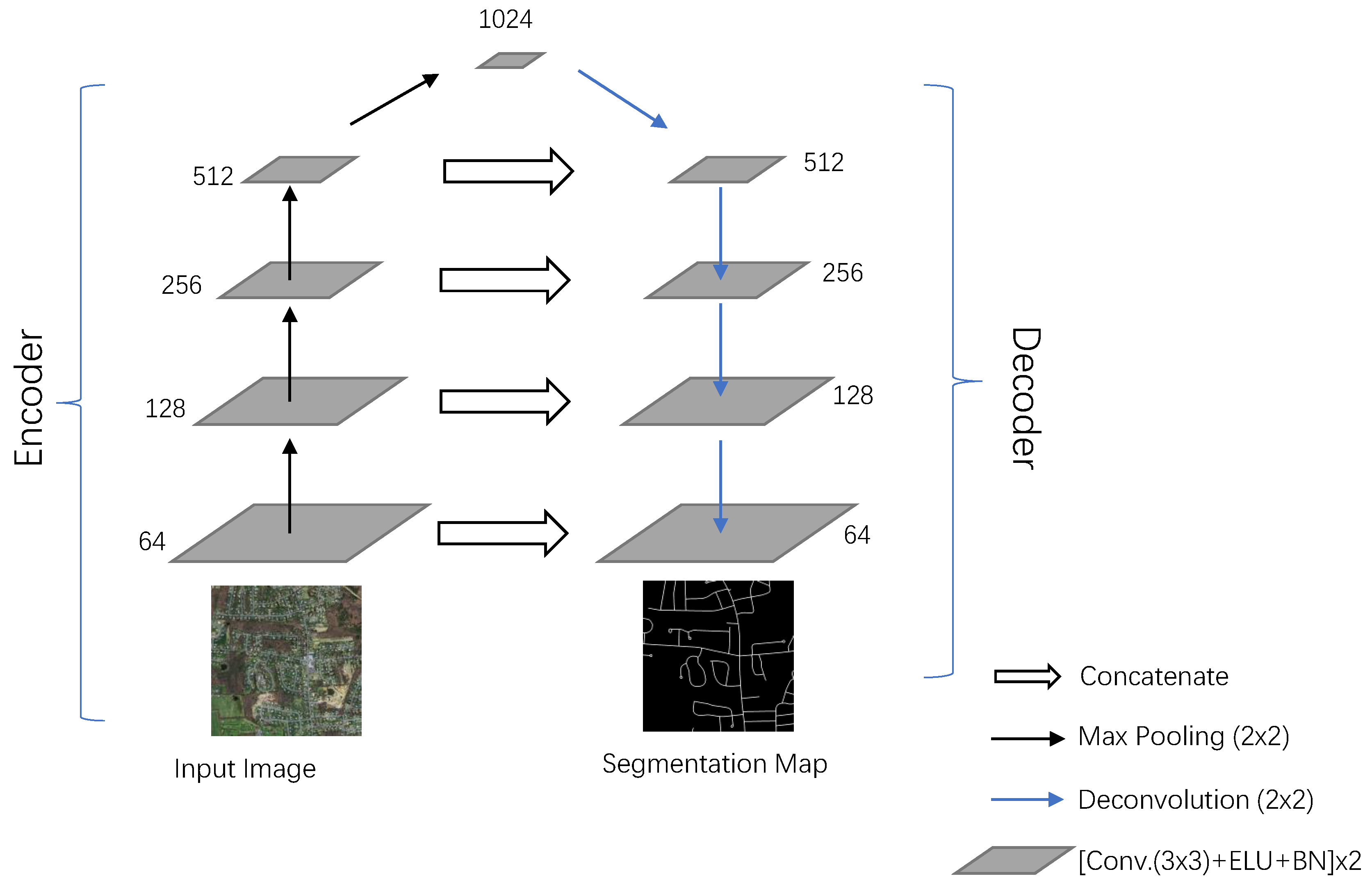
In this paper, we introduce an Encoder-Decoder network that is based on the architecture of the U-net, as shown in Figure 2. The U-net consists of two parts, an encoder and a decoder. The encoder part has the typical architecture of a convolutional network. It carries out repeated applications of two 3 × 3 convolutional layers, each of which are followed by an ELU activation function and a batch normalization layer. Each convolutional block follows a 2 × 2 max pooling operation for downsampling. The channels of the feature maps are doubled after each convolutional block. Every block in the decoder part consists of an upsampling operation that is achieved by a 2 × 2 deconvolution, concatenation with the corresponding feature map from the encoder part, and two 3 × 3 convolutions that are followed by an ELU and a batch normalization layer. The channels of the feature maps are halved after each upsampling process. In the final layer, a 1 × 1 convolution with a Sigmoid activation function is used to generate the output of the desired binary prediction.

In practice, we find that the Encoder-Decoder network’s hyperparameters, such as layers and convolution kernels, can be set to have flexibility in a certain range without affecting the road extraction results [31]. However, to facilitate the reproduction of this work, we built the network architecture on the basis of the classical U-net. Some modifications of the original U-net are proposed to improve the capacity of the network. Firstly, the activation of the rectified linear unit (ReLU) is replaced by the ELU. ReLU is a popular activation function in CNNs and is defined in Equation (1) [32].

$$ReLU\left(z\right)=max(0,z)$$

(1)

The ELU leads not only to a faster learning but also to a generalization performance that is significantly better than that of ReLU in deep networks [19]. It has also been reported that the ELU can increase the generalization performance and can improve the accuracy of classification in the remote sensing field [17,27]. Secondly, batch normalization is applied after each convolutional layer. Batch normalization can speed up the convergence of the training process and can avoid the vanishing gradient and exploding gradient problems.

2.1.2. Integration of ASPP

ASPP consists of several parallel atrous convolutions with different rates. It is a combination of atrous convolution and spatial pyramid pooling, and it can capture the contextual information at multiple scales for a more accurate classification. The road network not only contains abundant local details but also is a macro target with an almost infinite extension. Therefore, ASPP is needed to extract multiscale features for a road network extraction.

Atrous convolution is a powerful tool for controlling the resolution of the features computed by deep convolutional neural networks and for adjusting the receptive field to capture multiscale information. For each pixel $\mathit{i}$ on the output $\mathit{y}$ and filter $\mathit{w}$, atrous convolution is applied to the input $\mathit{x}$ as shown in Equation (2) [29]:

$$\mathit{y}\left[\mathit{i}\right]=\sum _{\mathit{k}}\mathit{x}[\mathit{i}+r·\mathit{k}]\mathit{w}\left[\mathit{k}\right]$$

(2)

where the atrous rate r determines the stride of sampling the input image. Atrous convolution is equivalent to convolving the input x with the filters produced by inserting $r-1$ zeros between two consecutive filter values. By adjusting the rate r, we can modify the receptive field of the filter.

We employed the ASPP module that is used in DeepLabv3 [24] to improve the proposed U-net network. It consists of four parallel atrous convolutions with different atrous rates. Specifically, the ASPP module consists of (a) one 1 × 1 convolution and three parallel 3 × 3 convolutions with rates of 6, 12, and 18, respectively and (b) an image-level feature that is produced by global average pooling. The resulting features from all of the branches are bilinearly upsampled to the input size and then concatenated and passed through another 1 × 1 convolution. ASPP is applied to the feature map produced by the encoder part, and the resulting feature map is fed into the decoder part, as shown in Figure 3.

2.2. SSIM Loss

The image signals of a road network are highly structured, and their pixels exhibit strong dependencies, especially on spatial relationships. However, normal metrics, such as cross-entropy, assign equal weights to each pixel and ignore the spatial information when evaluating the similarity between two images. The binary cross-entropy (BCE) loss function [32] of a general semantic segmentation is shown in Equation (3) and is used as the basic loss function in the proposed network.

$$L_{BCE}=-\frac{1}{N}\sum _{i=1}^N\left(y_i\left(log\widehat{y_i}\right)+\left(1-y_i\right)\left(1-log\widehat{y_i}\right)\right)$$

(3)

where $y_i$ is the ground truth of the ith pixel, $\widehat{y_i}$ is the prediction of the ith pixel, and N is the total number of pixels.

In addition, a problem often encountered in road segmentation is the blurriness of the results. The structural similarity index metric is a powerful tool for image quality assessment [26]. Generally, a higher SSIM means cleaner results [25]. This motivated us to improve the road segmentation quality by applying the SSIM as a loss function to train the network.

The SSIM evaluates the similarity between two images by comparing the luminance, contrast, and structure. Firstly, the luminance is compared by estimating the mean intensity. The luminance comparison function $l(\mathbf{x},\mathbf{y})$ is based on ${\mu }_x$ and ${\mu }_y$, where ${\mu }_x$ is defined by Equation (4).

$${\mu }_x=\frac{1}{n}\sum _{i=1}^N{x}_i$$

(4)

Secondly, the signal contrast can be estimated by using the standard deviation, which is given by Equation (5). Therefore, the contrast comparison $c(\mathbf{x},\mathbf{y})$ is a function of ${\sigma }_x$ and ${\sigma }_y$.

$${\sigma }_x={\left(\frac{1}{N-1}\sum _{i=1}^N{\left(x_i-{\mu }_x\right)}^2\right)}^{\frac{1}{2}}$$

(5)

Thirdly, the structure comparison $s(\mathbf{x},\mathbf{y})$ can be estimated by using the normalized signals denoted by $(\mathbf{x}-{\mu }_x)/{\sigma }_x$ and $(\mathbf{y}-{\mu }_y)/{\sigma }_y$. Therefore, the final similarity measure is a function that combines the three components, as defined in Equation (6).

$$S(\mathbf{x},\mathbf{y})=f\left(l\right(\mathbf{x},\mathbf{y}),c(\mathbf{x},\mathbf{y}),s(\mathbf{x},\mathbf{y}\left)\right)$$

(6)

To complete the definition of the similarity measure introduced in Equation (6), the three functions, $l(\mathbf{x},\mathbf{y})$, $c(\mathbf{x},\mathbf{y})$, and $s(\mathbf{x},\mathbf{y})$, as well as the combination $f(·)$, need to be defined. The luminance comparison is defined in Equation (7),

$$l(\mathbf{x},\mathbf{y})=\frac{2{\mu }_x{\mu }_y+C_1}{{\mu }_x^2+{\mu }_y^2+C_1}$$

(7)

where $C_1$ is a constant that is used to prevent instability when ${\mu }_x^2+{\mu }_y^2$ is close to zero.

The contrast comparison is defined in Equation (8):

$$c(\mathbf{x},\mathbf{y})=\frac{2{\sigma }_x{\sigma }_y+C_2}{{\sigma }_x^2+{\sigma }_y^2+C_2}$$

(8)

where $C_2$ is also a constant to prevent instability. Then, the structure comparison is estimated after normalizing the signals. The correlation (inner product) is a simple and effective measure for evaluating the structural similarity, which is defined in Equation (9), where $C_3$ is a constant that inhibits instability.

$$s(\mathbf{x},\mathbf{y})=\frac{{\sigma }_{xy}+C_3}{{\sigma }_x{\sigma }_y+C_3}$$

(9)

where ${\sigma }_{xy}$ is estimated according to Equation (10).

$${\sigma }_{xy}=\frac{1}{N-1}\sum _{i=1}^N(x_i-{\mu }_x)(y_i-{\mu }_y)$$

(10)

By combining the comparisons in Equations (7)–(9), we obtain the final measurement of the SSIM, which is defined in Equation (11).

$$SSIM(\mathbf{x},\mathbf{y})=[l{(\mathbf{x},\mathbf{y})}^{\alpha }·c{(\mathbf{x},\mathbf{y})}^{\beta }·s{(\mathbf{x},\mathbf{y})}^{\gamma }]$$

(11)

where $\alpha >0$, $\beta >0$, and $\gamma >0$ are parameters that are used to assign different weights to the three components. To simplify the expression, the parameters were set to be the same as in Reference [25], in which $\alpha =\beta =\gamma =1$ and $C_3=C_2/2$. This configuration is a default setting that is widely used; it not only provides a simple expression of the SSIM but also facilitates comparisons with similar works in the future. Therefore, Equation (11) can be rewritten as Equation (12).

$$SSIM(\mathbf{x},\mathbf{y})=\frac{(2{\mu }_x{\mu }_y+C_1)(2{\sigma }_{xy}+C_2)}{({\mu }_x^2+{\mu }_y^2+C_1)({\sigma }_x^2+{\sigma }_y^2+C_2)}$$

(12)

For the road segmentation problem, it is better to apply the SSIM locally rather than globally. This is because the road distribution is uneven in the image: Some areas contain a lot of local details, while others are blank. The global SSIM may overwhelm the effective local information and may reduce the efficiency of a similarity estimation. In addition, the ambiguous predictions of road extraction results are often local phenomena, so the statistics of local structural similarity are preferred.

The local statistics ${\mu }_x$, ${\sigma }_x$, and ${\sigma }_{xy}$ can be calculated by a square sliding window. In this work, we followed the approach used in Reference [25]. An $11\times 11$-unit circular symmetric Gaussian weighting matrix $\mathbf{w}$ with a standard deviation of 1.5 is used so that the quality maps exhibit a locally isotropic property. Therefore, the local statistics are modified according to Equations (13)–(15):

$${\mu }_x=\sum _{i=1}^N{w}_i{x}_i$$

(13)

$${\sigma }_x={\left(\sum _{i=1}^N{w}_i{\left(x_i-{\mu }_x\right)}^2\right)}^{\frac{1}{2}}$$

(14)

$${\sigma }_{xy}=\sum _{i=1}^N{w}_i\left(x_i-{\mu }_x\right)\left(y_i-{\mu }_y\right)$$

(15)

When training the network, it is necessary to condense the metrics into one function. Therefore, a mean SSIM (MSSIM) loss is used to evaluate the overall image quality [25], as defined in Equation (16).

$$MSSIM(\mathbf{X},\mathbf{Y})=\frac{1}{M}\sum _{j=1}^{M}SSIM({\mathbf{x}}_{\mathbf{j}},{\mathbf{y}}_{\mathbf{j}})$$

(16)

where $\mathbf{X}$ and $\mathbf{Y}$ are the ground truth and the predicted map, ${\mathbf{x}}_j$ and ${\mathbf{y}}_j$ are the image contents at the jth window, and M is the total number of local windows.

To integrate the SSIM loss with the end-to-end convolutional network, all of the local statistics can be computed by using a convolutional layer, as shown in Equations (17)–(19).

$${\mathit{\mu }}_x=Conv(\mathbf{X},\mathbf{w})$$

(17)

$${\mathit{\sigma }}_x^2=Conv(\mathbf{X}\odot \mathbf{X},\mathbf{w})-{\mathit{\mu }}_x\odot {\mathit{\mu }}_x$$

(18)

$${\mathit{\sigma }}_{xy}=Conv(\mathbf{X}\odot \mathbf{Y},\mathbf{w})-{\mathit{\mu }}_x\odot {\mathit{\mu }}_y$$

(19)

where $Conv(\mathbf{X},\mathbf{w})$ represents the convolution of $\mathbf{X}$ with $\mathbf{w}$ as the filter and ⊙ represents the Hadamard product between two tensors. The final loss function of the SSIM is given by Equation (20).

$$L_{SSIM}(\mathbf{X},\mathbf{Y})=-\frac{1}{M}\frac{(2{\mathit{\mu }}_{\mathit{x}}{\mathit{\mu }}_{\mathit{y}}+C_1)(2{\mathit{\sigma }}_{\mathit{xy}}+C_2)}{({{\mathit{\mu }}_{\mathit{x}}}^2+{{\mathit{\mu }}_{\mathit{y}}}^2+C_1)({{\mathit{\sigma }}_{\mathit{x}}}^2+{{\mathit{\sigma }}_{\mathit{y}}}^2+C_2)}$$

(20)

It is obvious that all of the math operations in the SSIM loss function are derivable, so it can be applied to an end-to-end convolutional network directly. We combined the SSIM loss with the BCE loss to train the network, and the final loss is calculated by Equation (21).

$$L=L_{BCE}+L_{SSIM}$$

(21)

2.3. Dataset and Preprocessing

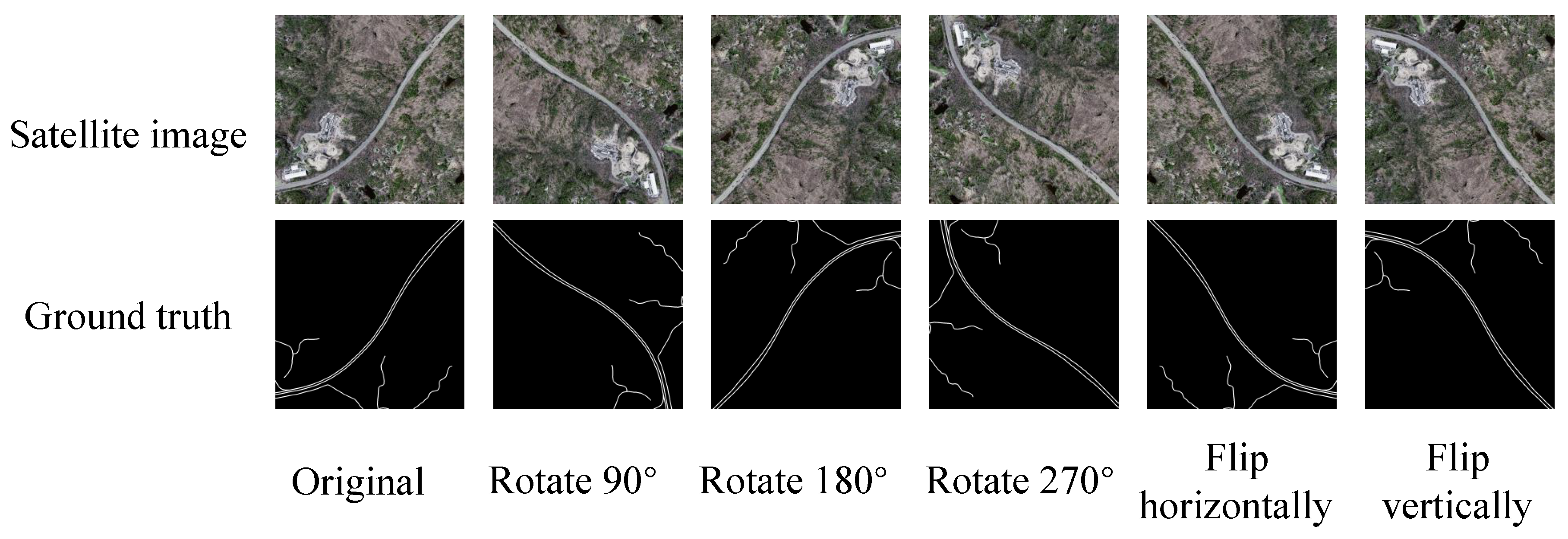
The dataset we employed in this study is the Massachusetts road dataset. It includes 1108 training images, 49 test images, and 14 validation images. Each image has a size of 1500 × 1500 and a resolution of 1 m/pixel. Because the training process in deep learning is data-hungry, we augmented the training data by rotating (90, 180, and 270 degrees) and flipping (horizontally and vertically), as shown in Figure 4. As a result, the training dataset has six times the number of images compared with the original dataset, with a total of 6648 images.

All of the images were preprocessed by cropping and normalization. Firstly, the input images are randomly cropped to 512 × 512. Cropping facilitates the downsampling operations and reduces the level of computation. Then, the cropped images were normalized to [−0.5,0.5] by 0–1 normalization and average value subtraction.

2.4. Evaluation Metrics

We employed recall, precision, and the F1-score as the evaluation metrics in this study. Recall and precision, which are also known as completeness and correctness in the remote sensing literature [33], are the most common metrics for evaluating road extraction results [9].

Since road segmentation is regarded as a semantic segmentation problem, the road pixels are positive and the background pixels are negative. Therefore, all of the predictions can be classified as one of four types: true positive (TP), true negative (TN), false positive (FP), and false negative (FN). TP represents the number of road pixels that are correctly classified. TN represents the number of background pixels that are correctly classified. FP is the number of background pixels that are classified as road. FN is the number of road pixels that are classified as background. These metrics are defined in Equations (22)–(24) [32].

$$recall=\frac{TP}{TP+FN}$$

(22)

$$precision=\frac{TP}{TP+FP}$$

(23)

$$F1=\frac{2\times precision\times recall}{precision+recall}=\frac{2TP}{2TP+FN+FP}$$

(24)

The precision is the fraction of predicted road pixels that are true roads, while the recall is the fraction of true road pixels that are correctly detected [9]. F1 is a combination of precision and recall. The same metrics have been used in similar works, such as References [13,14,17].

3. Experiment Results and Discussion

The proposed approach is based on the model of an enhanced U-net with two improvements: (a) ASPP integration to capture multiscale features and (b) the SSIM loss to improve the quality of the segmentation results. To validate our approach, we conducted experiments using three models: the baseline U-net, the ASPP-integrated U-net with normal loss, and the ASPP-U-net with SSIM loss. Except for the differences in the network architecture and loss function shown in

Table 1. The network configuration of the three compared models.

Model Name	ASPP Integration	Loss Function
Baseline U-net	No	$L_{BCE}$
ASPP-U-net	Yes	$L_{BCE}$
ASPP-U-net+SSIM	Yes	$L_{BCE}+L_{SSIM}$

, the three models’ hyperparameters, such as the convolutional layer, activation, and optimizer, are invariant to observe the effects of the proposed improvements.

3.1. Implementation Details

We utilized the Adam optimizer [34] to update the parameters. In the field of deep learning, Adam is a popular algorithm because it can achieve excellent results quickly. Empirical results have shown that the Adam algorithm has an excellent performance in practice and outperforms other optimization algorithms, such as SGD, RMSprop, and AdaGrad [35]. It can automatically adjust the learning rate during the iterations. For the Adam optimizer, some parameters should be initialized. We employed the default settings specified in Reference [34] because they have been tested for machine learning problems. The learning rate was set to $\alpha =0.001$, the exponential decay rates for the moment estimates were set to ${\beta }_1=0.9$ and ${\beta }_2=0.999$, and the small constant was $\epsilon ={10}^{-8}$.

All of the experiments were conducted using the PyTorch framework. The hardware environment of the experiments is a server with a CPU with the following specifications: Intel Xeon E5-2630 v4 × 15, 64 GB Memory, and an NVIDIA GeForce GTX 1080Ti(11G) GPU.

3.2. Discussion on Experimental Results

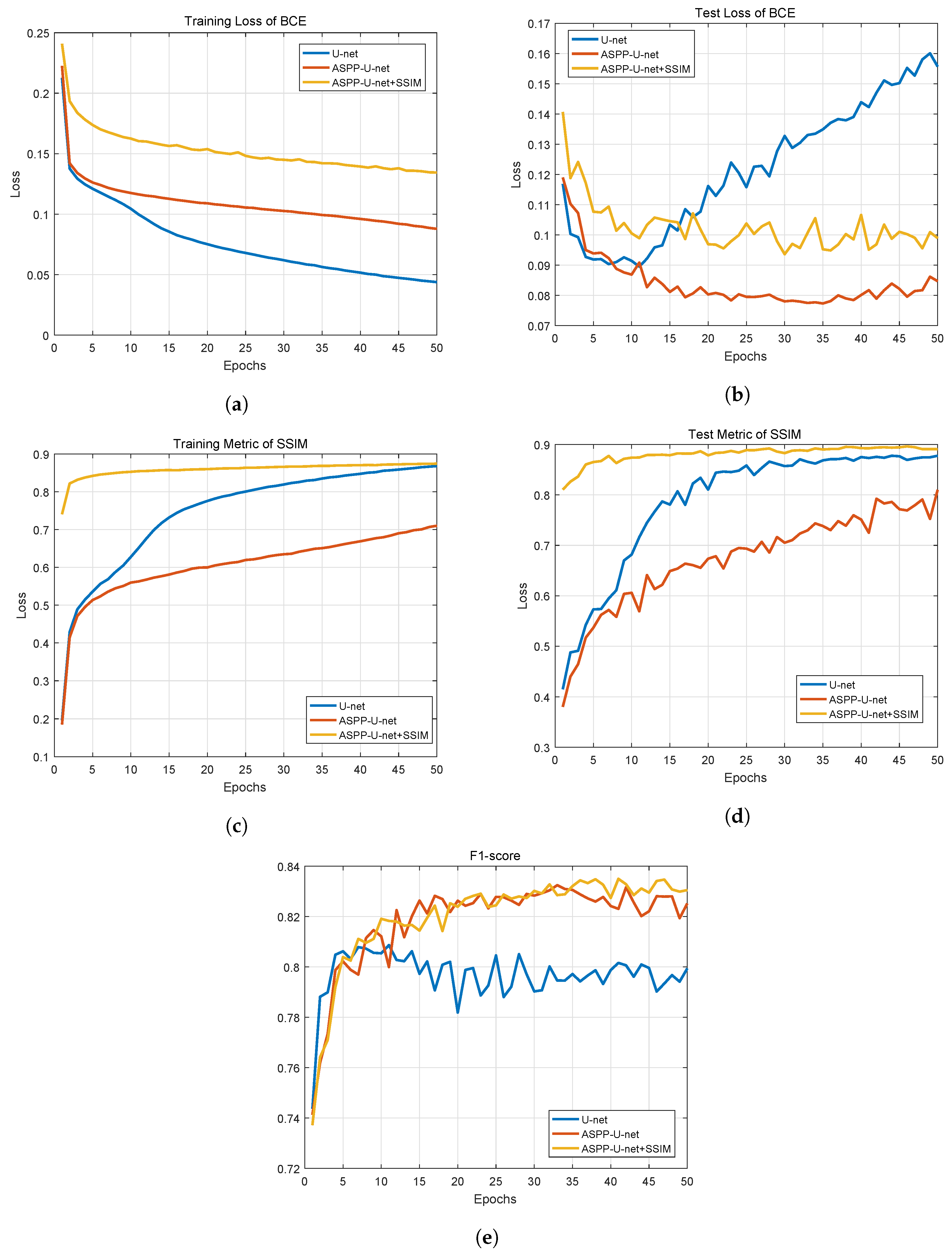
In order to determine the convergence and performance of the networks in the training process, some metrics were observed. By observing the mean losses of the training and test images displayed in Figure 5a,b, we can see that the baseline U-net achieves convergence before 15 epochs and begins overfitting with continuous training. The ASPP-U-net and ASPP-U-net-SSIM converge after about 30 epochs.

From evaluating the predictions of the test data in each epoch, we can observe the performance of the three models by the average MSSIM and mean F1-score metrics. Because of the overfitting phenomenon, the SSIM metric of the baseline U-net increases, as shown in Figure 5c,d. This is because the overfitting effect ignores some of the blurred targets and makes the segmentation map cleaner, but the accuracy begins to decline. From the test metrics in Figure 5d,e, we can see that an ASPP integration significantly improves the comprehensive metrics of road extraction and inhibits a premature convergence during training. Further, the SSIM loss function yields a higher SSIM metric, which means a better quality of the segmentation maps.

We adopted the trained models with the best F1-score performance. Their quantitative comparison is shown in

Table 2. The quantitative results of the comparative models: The performance results of the first three models listed are from several similar works that are cited in this paper, and the results of the last three models listed are from the experiments conducted in this study.

Model Name	Recall	Precision	F1-Score	Average MSSIM
FCN-4s [13]	66.0%	71.0%	68.4%	/
RSRCNN [14]	72.9%	60.6%	66.2%	/
ELU-SegNet-R [17]	78.0%	84.7%	81.2%	/
Baseline U-net	80.3%	82.0%	80.9%	0.716
ASPP-U-net	81.9%	84.9%	83.2%	0.730
ASPP-U-net-SSIM	80.5%	87.1%	83.5%	0.893

.

First, the performance of our baseline U-net is at the same level as that of the best model from the references, i.e., ELU-SegNet-R, and achieves the so-called “state-of-the-art”. It demonstrates that our baseline network represents the general level of the road extraction model.

ASPP integration aims to increase the accuracy of the network by capturing multiscale features. Table 2 shows that the ASPP-U-net outperforms the baseline U-net: the F1-score of ASPP-U-net is approximately 2.3% higher than that of the baseline U-net. The ASPP-U-net-SSIM performs about 2.6% better than the baseline U-net. These results prove that the strategy of integrating ASPP into the Encoder-Decoder network is effective.

The MSSIM values of the test images were averaged, and the F1-score of the ASPP-U-net is about 0.73, while that of the ASPP-U-net-SSIM is about 0.89. Although their F1-scores are similar, the ASPP-U-net-SSIM outperforms the ASPP-U-net in the SSIM metric. It is obvious that the SSIM loss function effectively improves the image quality of the results. It demonstrates the positive effect of the SSIM loss function from a quantitative perspective. In addition, it also shows that the F1-score cannot be used alone to evaluate the segmentation results and that the SSIM is a good complement.

In summary, it can be concluded that the two proposed strategies effectively improve the accuracy and quality of the road extraction results. In order to reveal the performance of the models and to interpret the quantitative metrics, the prediction results of the three networks are visualized.

ASPP is used to extract multiscale features and to improve the accuracy of classification. Both a general segmentation network and our ASPP-integrated network can correctly extract simple targets, so the advantages of our approach are not reflected by this process alone. However, when the local features of the target are blurred, the ASPP-integrated network can achieve a more accurate segmentation by taking advantage of the multiscale information. We illustrate this with some visual samples in Figure 6.

The local features of the sample images in Figure 6 are blurred, making their semantic segmentation difficult. Figure 6a presents a sample in which the road network is partly occluded, and Figure 6b,c shows a complex background around the road area. In the above three samples, the baseline U-net does not recognize the road network accurately or completely, and the results of the ASPP-U-net are better. It can be found that the proposed approach results in more True-Positive predictions than the baseline method, so the recall rate of the proposed model is higher. Figure 6d presents some other objects of which the features, such as rivers, are similar to those of the road network. The baseline U-net does not distinguish these areas from roads and classifies them as road targets, while the ASPP-U-net correctly classifies the region by drawing support from multiscale information. The proposed ASPP integration reduces the number of False-Positive predictions so that a higher precision is achieved.

It can be concluded that multiscale information can help to distinguish road targets with blurred features. Therefore, an ASPP integration can obtain discriminatory information to classify blurred areas and, thus, achieves a more accurate classification.

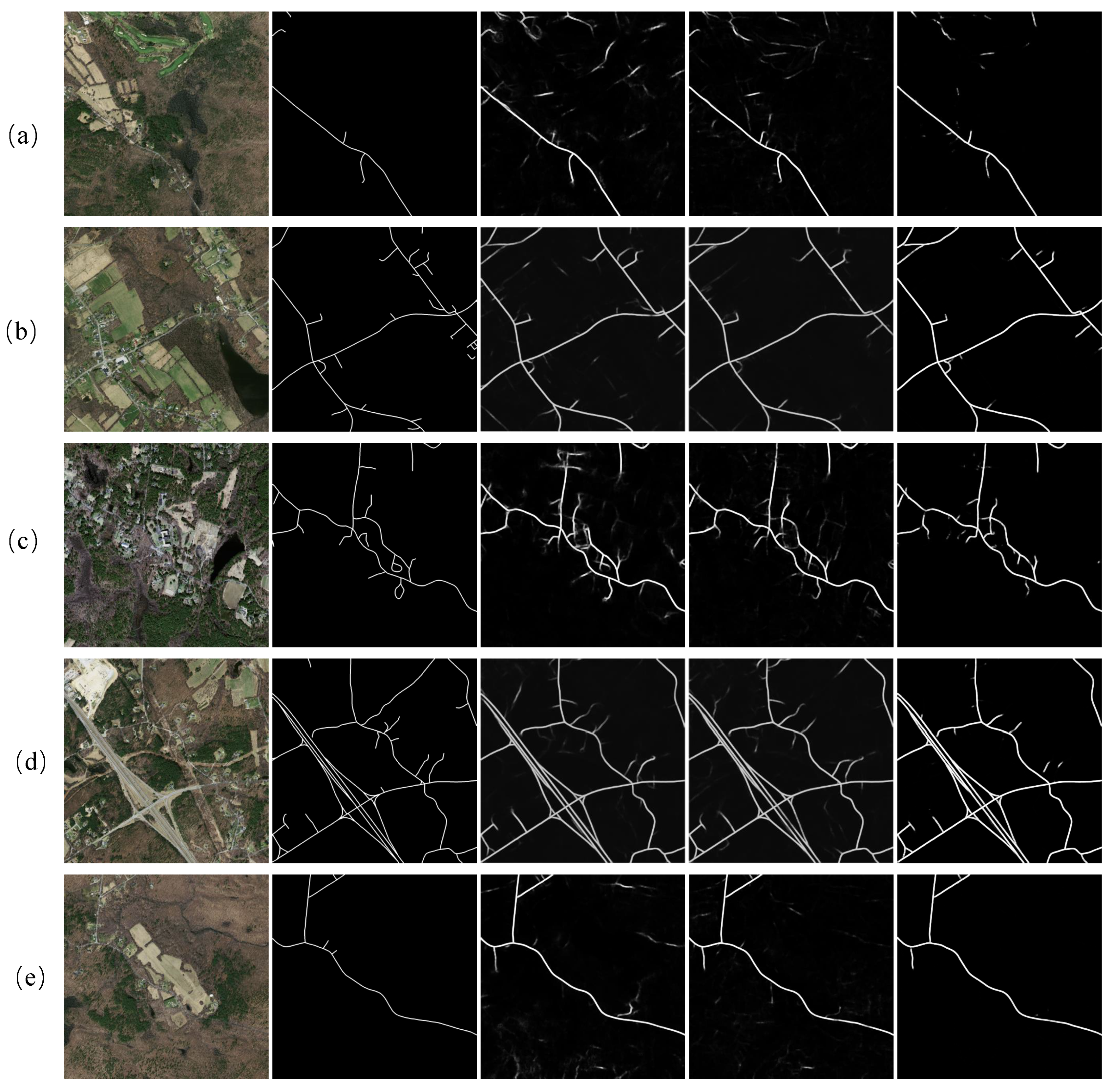
The SSIM loss function is used to prevent ambiguous segmentation and to improve the image quality of the extracted results. Generally, image quality is improved through post-processing methods, such as CRF. However, these methods deal with the extracted results and cannot be embedded in the end-to-end deep network. The SSIM loss function enables the network to directly produce segmentation maps with a satisfactory image quality. The effect of the SSIM loss function is shown in the visualization results in Figure 7.

Figure 7a presents the ambiguous segmentation map caused by false detection. Although it is a problem that occurs during the extraction and classification of features, the SSIM constraint removes these scattered false detections and improves the image quality. Figure 7b–d shows the ambiguous segmentation of areas that are adjacent to roads. Because of the inaccuracy of road width annotations, it is difficult for the network to accurately determine the road boundary, so compromised predictions are given. The application of the SSIM loss function can improve this situation and can make the extraction result clearer. Figure 7e illustrates an example of the result of the SSIM loss function’s removal of sporadic noise points. This figure demonstrates the additional effect of the loss function on improving the image quality.

Generally, the application of the SSIM loss function can remove ambiguous predictions and noise from the extraction results and can significantly improve the image quality. Compared with other post-processing methods, the SSIM loss function can be directly applied to end-to-end neural networks to improve the efficiency of obtaining high-quality results. A possible disadvantage of the SSIM loss function is that it may remove some correct predictions that have low confidence levels. Thus, although the SSIM loss function reduces false detections, the overall F1-score is not increased significantly.

4. Conclusions

The main purpose of this study was to improve the accuracy and quality of road extraction from remote sensing images. First, an approach that uses an ASPP-integrated Encoder-Decoder network was proposed. The ASPP module can capture multiscale features and can improve the accuracy of classification. The Encoder-Decoder network can recover the resolution of images completely and performs well in resolving segmenting details. We effectively improved the accuracy of road extraction by combining ASPP and the Encoder-Decoder network. Second, on the basis of the image quality assessment method using the SSIM, we designed a novel loss function to train the proposed network and effectively improved the image quality of the extracted results. The experiments were conducted using the Massachusetts road dataset. The quantitative experimental metrics and visual experimental results all demonstrated that the ASPP-integrated network can effectively improve the accuracy of road extraction and that the SSIM loss function can improve the image quality significantly. Our approach outperformed the compared “state-of-the-art” methods not only in F1, precision, and recall but also in the SSIM image quality metric. Our approach achieved an F1-score of 83.5%, which is 15% higher than that of the FCN methods [13,14] and 2% higher than that of SegNet [17] and the baseline U-net. For the SSIM loss, our approach realized an SSIM index of 0.893, which is about 0.18 higher than that of the baseline U-net.

In the future, we will aim to constrain the topological features of the road in the training of the deep neural network and will improve the topological structure of the road extraction results. This research can be carried out from the aspects of the network structure, components, and the loss function.

References

1. Steger, C. An unbiased detector of curvilinear structures. IEEE Trans. Pattern Anal. Mach. Intell. 1998, 20, 113–125. [Google Scholar] [CrossRef] [Green Version]
2. Zhou, Y.T.; Venkateswar, V.; Chellappa, R. Edge detection and linear feature extraction using a 2-D random field model. IEEE Trans. Pattern Anal. Mach. Intell. 1989, 11, 84–95. [Google Scholar] [CrossRef]
3. Koutaki, G.; Uchimura, K. Automatic road extraction based on cross detection in suburb. Electron. Imaging 2004, 36, 2–9. [Google Scholar]
4. Hu, J.; Razdan, A.; Femiani, J.C.; Cui, M.; Wonka, P. Road network extraction and intersection detection from aerial images by tracking road footprints. IEEE Trans. Geosci. Remote Sens. 2007, 45, 4144–4157. [Google Scholar] [CrossRef]
5. Ravanbakhsh, M.; Heipke, C.; Pakzad, K. Road junction extraction from high-resolution aerial imagery. Photogramm. Rec. 2010, 23, 405–423. [Google Scholar] [CrossRef]
6. Marikhu, R.; Dailey, M.N.; Makhanov, S.; Honda, K. A Family of quadratic snakes for road extraction. In Proceedings of the 8th Asia Conference on Computer Vision, Tokyo, Japan, 18–22 November 2007; pp. 85–94. [Google Scholar]
7. Wegner, J.D.; Montoya-Zegarra, J.A.; Schindler, K. A higher-order CRF model for road network extraction. In Proceedings of the IEEE Computer Society Conference on Computer Vision and Pattern Recognition, Portland, OR, USA, 23–28 June 2013; pp. 1698–1705. [Google Scholar]
8. Mnih, V.; Hinton, G.E. Learning to detect roads in high-resolution aerial images. In Proceedings of the European Conference on Computer Vision, Heraklion, Crete, Greece, 5–11 September 2010; pp. 210–223. [Google Scholar]
9. Mnih, V. Machine Learning for Aerial Image Labeling. Ph.D. Thesis, University of Toronto, Toronto, ON, Canada, 2013. [Google Scholar]
10. Wang, J.; Song, J.; Chen, M.; Yang, Z. Road network extraction: A neural-dynamic framework based on deep learning and a finite state machine. Int. J. Remote Sens. 2015, 36, 3144–3169. [Google Scholar] [CrossRef]
11. Alshehhi, R.; Marpu, P.R.; Woon, W.L.; Mura, M.D. Simultaneous extraction of roads and buildings in remote sensing imagery with convolutional neural networks. ISPRS J. Photogramm. Remote Sens. 2017, 130, 139–149. [Google Scholar] [CrossRef]
12. Long, J.; Shelhamer, E.; Darrell, T. Fully convolutional networks for semantic segmentation. In Proceedings of the IEEE Conference on Computer Vision and Pattern Recognition, Boston, MA, USA, 7–12 June 2015; pp. 3431–3440. [Google Scholar]
13. Zhong, Z.; Li, J.; Cui, W.; Jiang, H. Fully convolutional networks for building and road extraction: Preliminary results. In Proceedings of the IEEE International Geoscience and Remote Sensing Symposium (IGARSS), Beijing, China, 10–15 July 2016; pp. 1591–1594. [Google Scholar]
14. Wei, Y.; Wang, Z.; Xu, M. Road structure refined CNN for road extraction in aerial image. IEEE Geosci. Remote Sens. Lett. 2017, 14, 709–713. [Google Scholar] [CrossRef]
15. Ronneberger, O.; Fischer, P.; Brox, T. U-Net: Convolutional networks for biomedical image segmentation. In Proceedings of the Medical Image Computing and Computer-Assisted Intervention, Munich, Germany, 5–9 October 2015; pp. 234–241. [Google Scholar]
16. Cheng, G.; Wang, Y.; Xu, S.; Wang, H.; Xiang, S.; Pan, C. Automatic road detection and centerline extraction via cascaded End-to-End convolutional neural network. IEEE Trans. Geosci. Remote Sens. 2017, 55, 3322–3337. [Google Scholar] [CrossRef]
17. Panboonyuen, T.; Jitkajornwanich, K.; Lawawirojwong, S.; Srestasathiern, P.; Vateekul, P. Road segmentation of remotely-Sensed images using deep convolutional neural networks with landscape metrics and conditional random fields. Remote Sens. 2017, 9, 680. [Google Scholar] [CrossRef]
18. Badrinarayanan, V.; Kendall, A.; Cipolla, R. Segnet: A Deep convolutional encoder-decoder architecture for image segmentation. arXiv 2015, arXiv:1511.00561. [Google Scholar] [CrossRef] [PubMed]
19. Clevert, D.A.; Unterthiner, T.; Hochreiter, S. Fast and accurate deep network learning by exponential linear units (ELUs). arXiv 2015, arXiv:1511.07289. [Google Scholar]
20. Zhang, Z.; Liu, Q.; Wang, Y. Road extraction by deep residual U-Net. IEEE Geosci. Remote Sens. Lett. 2018, 15, 749–753. [Google Scholar] [CrossRef]
21. He, K.; Zhang, X.; Ren, S.; Sun, J. Deep residual learning for image recognition. In Proceedings of the IEEE Conference on Computer Vision and Pattern Recognition, Las Vegas, NV, USA, 27–30 June 2016; pp. 770–778. [Google Scholar]
22. Mosinska, A.; Márquez-Neila, P.; Kozinski, M.; Fua, P. Beyond the pixel-wise loss for topology-aware delineation. In Proceedings of the 2018 IEEE/CVF Conference on Computer Vision and Pattern Recognition, Munich, Germany, 8–14 September 2018; pp. 3136–3145. [Google Scholar]
23. Simonyan, K.; Zisserman, A. Very deep convolutional networks for large-scale image recognition. In Proceedings of the International Conference on Learning Representations, San Diego, CA, USA, 7–9 May 2015. [Google Scholar]
24. Chen, L.C.; Papandreou, G.; Schroff, F.; Adam, H. Rethinking atrous convolution for semantic image segmentation. arXiv 2017, arXiv:1706.05587. [Google Scholar]
25. Zhou, W.; Alan Conrad, B.; Hamid Rahim, S.; Simoncelli Eero, P. Image quality assessment: from error visibility to structural similarity. IEEE Trans. Image Process. 2004, 13, 600–612. [Google Scholar]
26. Søgaard, J.; Krasula, L.L.; Shahid, M.; Temel, D.; Søgaard, J.; Krasula, L.L.; Shahid, M.; Temel, D.; Brunnström, K.; Razaak, M. Applicability of Existing Objective Metrics of Perceptual Quality for Adaptive Video Streaming. Electron. Imaging 2016, 13, 1–7. [Google Scholar] [CrossRef]
27. Shrestha, S.; Vanneschi, L. Improved Fully convolutional network with conditional random fields for building extraction. Remote Sens. 2018, 10, 1135. [Google Scholar] [CrossRef]
28. Ioffe, S.; Szegedy, C. Batch normalization: Accelerating deep network training by reducing internal covariate shift. In Proceedings of the Iernational Conference on Machine Learning, Lille, France, 6–11 July 2015; pp. 448–456. [Google Scholar]
29. Chen, L.C.; Zhu, Y.; Papandreou, G.; Schroff, F.; Adam, H. Encoder-Decoder with atrous separable convolution for semantic image segmentation. arXiv 2018, arXiv:1802.02611. [Google Scholar]
30. Iglovikov, V.; Mushinskiy, S.; Osin, V. Satellite Imagery Feature Detection using Deep Convolutional Neural Network: A Kaggle Competition. arXiv 2017, arXiv:1706.06169. [Google Scholar]
31. He, H.; Wang, S.; Yang, D.; Wang, S.; Liu, X. A road extraction method for remote sensing image based on Encoder-Decoder network. Acta Geod. Cartogr. Sin. 2019, 48, 330–338. [Google Scholar]
32. Goodfellow, I.; Bengio, Y.; Courville, A. Deep Learning; MIT Press: Cambridge, UK, 2016. [Google Scholar]
33. Wiedemann, C.; Heipke, C.; Mayer, H.; Jamet, O. Empirical Evaluation of Automatically Extracted Road Axes. In Empirical Evaluation Techniques in Computer Vision; IEEE Computer Society Press: Los Alamitos, CA, USA, 1998; pp. 172–187. ISBN 978-0-818-68401-2. [Google Scholar]
34. Kingma, D.; Ba, J. Adam: A method for stochastic optimization. arXiv 2014, arXiv:1412.6980. [Google Scholar]
35. Ruder, S. An overview of gradient descent optimization. arXiv 2016, arXiv:1609.04747. [Google Scholar]
Figure 1. A general scheme of training the deep segmentation network.
Remotesensing 11 01015 g001
Figure 2. A brief illustration of the improved U-net structure: The left-side blocks form the encoder part, in which the channels of the feature maps are doubled from 64 to 1024. The blocks on the right side constitute the decoder part, in which the resolution of the feature maps is gradually recovered by upsampling and gathering information from the encoder feature maps. Finally, a binary segmentation map that has the same resolution as the input image is produced as the road extraction result.
Remotesensing 11 01015 g002
Figure 3. The improved U-net with atrous spatial pyramid pooling (ASPP) integration: The ASPP module is inserted after the bottleneck of the Encoder-Decoder network. This means that the feature map generated by the encoder is processed by using ASPP, and then, the result is fed into the decoder.
Remotesensing 11 01015 g003
Figure 4. An example of augmenting the training data by rotating and flipping.
Remotesensing 11 01015 g004
Figure 5. The training metrics of the three different experiments. (a) is the BCE loss of the training process, and (b) is the BCE loss of the test predictions. (c) is the SSIM metric in training process, and (d) is the SSIM metric of the test predictions. (e) is the mean F1-score of the test predictions.
Remotesensing 11 01015 g005
Figure 6. Visual comparisons between the baseline U-net and ASPP-integrated U-net using test samples from the Massachusetts road dataset: The results are binarized using a threshold of 0.5. For each row in (a)–(d), it contains an input image, a ground truth image and two result maps of a sample region.
Remotesensing 11 01015 g006
Figure 7. Visualization results of three models in the test set of the Massachusetts road dataset: The brightness of the results represents the confidence of the predicted results. For each row in (a)–(e), it contains an input image, a ground truth image and three result maps of a sample region.
Remotesensing 11 01015 g007