Abstract
Growing interest in the proximal sensing of sun-induced chlorophyll fluorescence (SIF) has been boosted by space-based retrievals and up-coming missions such as the FLuorescence EXplorer (FLEX). The European COST Action ES1309 “Innovative optical tools for proximal sensing of ecophysiological processes” (OPTIMISE, ES1309; https://optimise.dcs.aber.ac.uk/) has produced three manuscripts addressing the main current challenges in this field. This article provides a framework to model the impact of different instrument noise and bias on the retrieval of SIF; and to assess uncertainty requirements for the calibration and characterization of state-of-the-art SIF-oriented spectroradiometers. We developed a sensor simulator capable of reproducing biases and noises usually found in field spectroradiometers. First the sensor simulator was calibrated and characterized using synthetic datasets of known uncertainties defined from laboratory measurements and literature. Secondly, we used the sensor simulator and the characterized sensor models to simulate the acquisition of atmospheric and vegetation radiances from a synthetic dataset. Each of the sensor models predicted biases with propagated uncertainties that modified the simulated measurements as a function of different factors. Finally, the impact of each sensor model on SIF retrieval was analyzed. Results show that SIF retrieval can be significantly affected in situations where reflectance factors are barely modified. SIF errors were found to correlate with drivers of instrumental-induced biases which are as also drivers of plant physiology. This jeopardizes not only the retrieval of SIF, but also the understanding of its relationship with vegetation function, the study of diel and seasonal cycles and the validation of remote sensing SIF products. Further work is needed to determine the optimal requirements in terms of sensor design, characterization and signal correction for SIF retrieval by proximal sensing. In addition, evaluation/validation methods to characterize and correct instrumental responses should be developed and used to test sensors performance in operational conditions.
1. Introduction
The estimation of passive sun-induced chlorophyll fluorescence (SIF) has interested the remote sensing community for some decades due to its potential to monitor photosynthesis [1]. SIF is one of the alternative pathways that absorbed photons can take in photosynthetic machinery, and therefore, is linked to photosynthetic activity and stress [2]. In the last decade, remote sensing of SIF has made great progress. On one side, the first SIF retrievals from space were achieved from meteorological satellites [3,4,5]. On the other side, a lot of effort has been invested in the preparation of the FLEXmission [6,7]; which has been selected as the European Space Agency’s (ESA) 8th Earth Explorer mission and is planned to be launched in 2022. These developments have also boosted the interest of the near-ground remote sensing (proximal sensing) community in the retrieval of SIF. The contribution of this community will be of great value since SIF is a challenging signal to retrieve as well as to interpret. Proximal SIF retrievals can be combined with ancillary measurements at comparable, temporal and spatial scales, to improve the interpretation and understanding of the SIF signal. This will also aid down-scaling to understand leaf level processes and the validation of remote SIF products [8,9,10]. Fifteen years ago, most of the spectroradiometers featured spectral resolutions too coarse for an absolute proximal quantification of SIF (e.g., full width half maximum (FWHM) ≥ 1 nm); and most of the retrievals were based on multispectral Fraunhofer Line Depth (FLD) methods [1,11]. Since then, new portable field spectroradiometers have been developed well as their use has spread in the scientific community. These spectroradiometers feature higher spectral resolutions (e.g., FWHM ≤ 0.39 nm), higher signal-to-noise ratios (e.g., SNR ~ 1000:1), and extended dynamic ranges of 200,000 counts, which enable SIF to be retrieved in different atmospheric dark lines from the same measurement. Nowadays these spectroradiometers are considered to be state-of-the-art instrumentation for the proximal sensing of SIF. At a European level, these developments have been partly supported by scientific collaborative efforts within European cooperation in science and technology (COST) actions (https://www.cost.eu) (i.e., ES0903 and ES1309). Wider international networks have also contributed (e.g., SPECNET, https://www.specnet.info). In the last four years, the wider scientific network involved in the COST Action ES1309 (OPTIMISE) has collaborated specifically to address challenges in the proximal sensing of SIF. This work has included instrumentation; measurement protocols; and retrieval techniques. To make the results of these efforts available to a wider audience, the OPTIMISE community has compiled three papers summarizing their shared experience on instrumental characterization (this article), measurement setups and protocols [12] and retrieval methods [13]. These review articles aim to summarize the state-of-the-art, guidelines, current needs, and future directions concerning spectroradiometric measurements for SIF retrieval. The intention is to provide an update to the previous review performed a decade ago by Meroni et al. [1].
Since reference [1] was written, two new generations of spectroradiometric systems for the retrieval of SIF have been developed and their use extended to operate at canopy level. These systems are characterized by having custom designed spectroradiometers dedicated to the retrieval of SIF; featuring: (1) narrow spectral ranges (100–200 nm) between the red and the near infrared (NIR) regions, and (2) very high spectral resolutions (e.g., FWHM ≤ 0.39 nm, and <0.2 nm sampling intervals). These systems are often complemented by a visible and near-infrared (VNIR) spectrometer, used for the determination of hemispherical conical reflectance factors as well as spectral indices such as the Photochemical Reflectance Index (PRI) [14]. Earlier systems featured sub-nanometric FWHM but poor SNR (e.g., < 1000:1); these systems usually relied on sensors such as the HR or USB series produced by Ocean Optics (Dunedin, FL, USA) or similar instruments [8,15,16,17,18,19,20,21,22,23,24]. A second generation arrived by the replacement of the sensor dedicated to SIF retrieval by spectrometers with high SNR (~1000:1), such as the QE series from Ocean Optics or similar. One of the advantages of these instruments is the thermal stabilization of the detector. Two systems incorporating these spectrometers result partly from the exchanges and collaborative efforts carried out under the umbrella of the COST Action OPTIMISE: the FLuorescence bOX (FloX, JB Hyperspectral, Dusseldorf, Germany) [25] and the Piccolo Doppio (a collaborative effort lead by GeoSciences, University of Edinburgh) [26]; similar systems were developed by other teams [27,28,29,30].
SIF constitutes a small fraction of the up-welling radiance observed by an optical sensor; in absolute terms, this signal constitutes only a few (≤5) mW/m2/sr/nm [1,31] to a signal that may exceed 300 mW/m2/sr/nm [17]. This makes SIF retrieval and interpretation very sensitive to uncertainties, which can lead to spurious results and erroneous conclusions. Sources of error in the proximal sensing of SIF can be separated into three groups, as they are related to: (1) instrumentation—sensors introduce biases and noise in the recorded signal; (2) measurement procedure—this can induce significant errors in observations or assist avoiding them (in addition inadequate measurement procedures can limit or prevent the integration of SIF estimates with other variables in space and time and through different scales); (3) retrieval; different retrieval algorithms can lead to different values and each varies in sensitivity to uncertainties. These topics are addressed in the three related articles arising from the cooperation run in the context of the COST Action OPTIMISE in this special issue: the current paper, and references [12] and [13], respectively.
Spectroradiometers are passive sensors spectrally sensitive to electro-magnetic radiation, as well as other environmental variables, which are radiometric and spectrally calibrated. Therefore, the pixel spectral response and the magnitude of the signal generated by the sensor can be expressed in internationally recognized units and traced to known standards. However this relationship, between the natural phenomena that is required to be measured (the measurand) and the recorded signal, is always sensitive to uncertainties and the instrument’s responses to other factors (e.g., signal magnitude, sensor temperature, etc.). Every spectral band is defined by its spectral response function (SRF); which is commonly approximated by a Gaussian function and therefore described by the center wavelength (λc) and the FWHM. The radiometric calibration converts spectrometer outputs (raw data, generally digital numbers or micro volts) into internationally standardized (SI) physical units—most commonly of spectral radiance [W/m2/sr/nm] or irradiance [W/m2/nm] [32]. Every measurement is accompanied by an uncertainty, defined as a “parameter, associated with the result of a measurement, that characterizes the dispersion of the values that could reasonably be attributed to the measurand” [33]. Calibration parameters, therefore, include some uncertainties. These calibration uncertainties can be estimated in the laboratory, and, subsequently, propagated through to operational measurements. The metrological traceability is defined as the “property of a measurement result whereby the result can be related to a reference through a documented unbroken chain of calibrations, each contributing to the measurement uncertainty” [33]. Traceability and uncertainty propagation are rarely considered in proximal sensing applications, both in the laboratory and especially in the field. However, since SIF is a weak signal sensitive to several sources of error [13,34], in this paper the propagation of uncertainties is necessary to determine which observations can provide reliable SIF retrievals that can be understood according to the precision and accuracy requirements of each application or scientific question.
Several phenomena can modify the relationships established between calibration and measurements made by the sensor. Some of these are related to the unavoidable degradation of detectors due to age and usage, an issue that imposes the need of periodical recalibration of the instruments. Some others factors modify sensor response as a function of sensor configuration, radiometric and environmental variables. Temperature is known to modify the silicon (Si) photo-response [35,36,37], the dark noise levels [35,36,38], or the frequency of the clock used to set the integration time [39]. Temperature can be measured in the detector using temperature probes, and therefore used to fit sensor models that correct their effects [35,36]. However, if only sensor body or ambient temperatures can be measured, gradients and temporal shifts related to the propagation of heat through, and temperature gradients across, the instrument and photodetector should be considered [40,41]. Temperature also induces dimensional modifications of the spectrometer’s optical and mechanical components; which implies changes in the spectral features of the system (λc, FWHM). These changes can strongly affect the radiance values observed inside and outside the dark absorption lines used to retrieve SIF [34]. Other sources of error are related with non-linear responsivity of the sensor caused by supra-responsivity [42,43,44]; saturation or early leakage in antiblooming switches [45]; non-linear signal transfer and transformation processes taking place in the sensor electronics [46,47,48]; or charge leakage during the readout phase [49,50]. Non-linearity can be corrected [50,51], or better prevented by optimizing the integration time such that signals remain outside of the less linear regions of the response. Cosine diffusers and calibrated reflectance reference panels used to measure the down-welling irradiance are expected to provide a cosine directional response (DR). However, some instruments may deviate from this function and, even if characterization is possible [36,52,53,54], accurate correction requires knowledge on the diffuse fraction of the observed down-welling irradiance [36,54] which varies in the spectral and directional domains.
Only a few works have considered and analyzed the impact of some of these instrumental sources of error on the retrieval of SIF. These works have mainly focused on the effects of noise, spectral configuration and spectral shift on different retrieval methods, and did not address propagation of uncertainties, other than for sensor noise [34,55,56]. This article aims to contribute to the understanding of some of the instrumental sources of error on the retrieval of SIF, focusing on the latest generation sensors available and on a single SIF retrieval method. This work does not attempt to be exhaustive, but rather focuses on some of the best known instrumental responses and on the use of a framework that could be applied in the future for similar analyses.
2. Materials and Methods
2.1. Data Simulation for Fluorescence Retrieval
In order to test the effect of different uncertainties in the retrieval of SIF under controlled conditions, we produced a synthetic dataset of radiant fluxes: the Vegetation Dataset. Bottom of the atmosphere (BOA) down-welling irradiance spectra were generated for unvarying atmospheric conditions at different solar zenith angles (θs) between 0.00° and 83.32°. Direct (E↓dir) and diffuse (E↓diff) very high spectral resolution irradiances (FWHM = 0.005 nm) were produced by the radiative transfer code MOMO [57] between 500 and 800 nm, and combined as a function of θs (Equation (1)).
where E↓tot is the total BOA down-welling irradiance. For most of the analyses in the manuscript, we used the irradiance spectra simulated for θsun = 29.80° (angles were taken as available in a look-up-table generated in the FLUSS project). Irradiances at different θsun were only used for the study of the diffuser directional response (see Section 2.3.6). A typical vegetation reflectance factor (R) and top of the canopy SIF radiance in the observation direction (F↑) spectra were generated using the model SCOPE [58] version 1.7. For simplicity we assumed a Lambertian vegetation canopy, limiting the analysis of directional effects to those induced by the sensor. R and F↑ smooth spectra were interpolated using cubic splines to MOMO spectral bands in order to compute at-nadir BOA up-welling apparent radiance (L↑app)—which combines both reflected and emitted radiances—as in Equation (2):
From these datasets we simulated spectra observed by a typical field spectroradiometer dedicated to the retrieval of SIF in both major telluric oxygen absorption bands: O2-B (~687.0 nm) and O2-A (~760.4 nm) [1]. This spectroradiometer would be very similar to one of the systems most frequently used for proximal sensing of SIF in the last years, the Ocean Optics QE Pro (Ocean Optics, Dunedin, FL, USA). However, we would like to emphasize that this study does not aim to exactly replicate the characteristics of this specific sensor; and the topics under analysis are common to any spectroradiometric system (including not only the spectroradiometer, but also fibers, fore optics, multiplexers etc.), each featuring unique responses to the different factors analyzed. The simulated spectroradiometer featured 1024 channels between 650 and 810 nm, with a spectral sampling interval of ~ 0.1564 nm and FWHM = 0.32 nm. Constant values were chosen for simplicity, but these actually vary along the detector. The system operates in a dual-field-of-view configuration; which means that the up-welling and down-welling fluxes are sampled sequentially by the same detector. In this case, we assumed that the first was sampled by a bare optical fiber tip and the second through a hemispherical cosine corrected diffuser. This configuration would be usual for tower-based or drone-borne automated, as well as for manually operated systems.
2.2. Sensor Simulator
In order to model and reproduce the measurement process and to include instrumental-induced biases and uncertainties we developed a Sensor Simulator. The Sensor Simulator was capable of optimizing integration time (tint) according to the radiance observed so that the maximum digital signal reached 175,000 digital numbers (DN) (87.5% of the saturation level: 200,000 DN). It also produced dark current (N0,λ)—the inherent electrical noise in all electronic sensors—and added sensor noise according to the signal level and transformed the digital signal (Nλ) to physical units and vice versa. For convenience, in this article we assumed , and operated the sensor simulator in spectral radiance units (Lλ). The transformation of the digital signal to radiances was carried out as follows (Equation (3)):
where gλ is the radiometric calibration coefficient and λ denotes the spectral component of the variables. A set of radiometric calibration coefficients of a FloX (JB Hyperspectral, Dusseldorf, Germany) spectroradiometric system was used for this simulator. We also generated a model predicting sensor random noise in digital numbers (Appendix A) as a function of tint and of the ratio ; a variable proportional to Lλ (Equation (3)). “Measured” radiances were generated applying spectral convolution [59] to L↑app and E↓tot, assuming Gaussian SRF [60]. Figure 1 shows the original and the convolved radiances, as well as the F↑ used to generate these datasets.
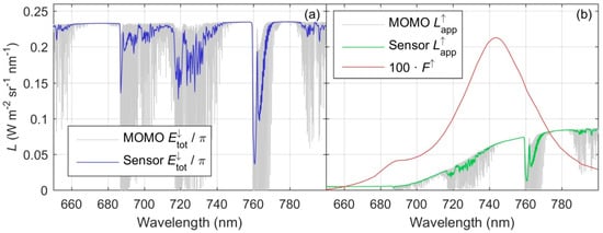
Figure 1.
(a) Bottom of the atmosphere (BOA) down-welling simulated radiances; (b) BOA up-welling simulated radiances and top of the canopy sun-induced chlorophyll fluorescence (SIF) radiance emission. F↑ is scaled by a factor of 100 in the plot.
From this dataset and the datasets generated in the following analyses (Section 2.3), we retrieved F↑ in both O2-A and O2-B bands using Spectral Fitting Methods from the FieldSpectroscopyDP R package. The package is available on the GitHub platform at https://github.com/tommasojulitta under GNU v3.0 [61]. These results were compared with simulated F↑ values to assess the impact of the different uncertainties and instrumental biases on SIF retrieval in both oxygen bands. Notice that this work does not aim to test the performance of different retrieval algorithms and uses only one of them. Further analyses on the performance of different retrieval methods can be found in this issue [13]. F↑ in the O2-B and O2-A bands for the spectra simulated with θs = 29.80° was 0.411 mW/m2/sr/nm and 1.427 mW/m2/sr/nm, respectively. F↑ retrieved in the O2-B and O2-A bands is labeled with subscripts 687 and 760 through the paper. However, notice that the bands selected for the retrieval depend on the algorithms used, which often rely on the band with the minimum radiance value within the absorption feature [13]. The selected band can vary according to the spectral configuration of the sensor and the spectral shifts induced and simulated in different analyses (Section 2.3.1 and Section 2.3.2).
2.3. Characterization of Sensor Models and Instrumental Uncertainties
Figure 2 summarizes the dataflow of the different datasets and models generated as well as the uncertainty propagation. Uncertainty propagation methods are described in Section 2.4.
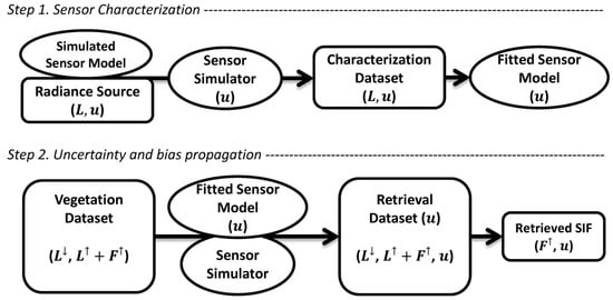
Figure 2.
Data flowchart representing the combination of the different datasets (rectangles) and models (ellipses) used in the different simulations of this article. The radiometric variables contained in each dataset are indicated between brackets. Models that simulate uncertainty propagation and those datasets that include uncertainty distributions present the symbol (u) between brackets. A detailed description of the sensor simulator is shown in Appendix A.
In order to analyze the impact of different instrumental error sources on SIF retrieval, we first simulated the characterization and calibration of the sensor simulator as follows (Step 1 in Figure 2):
- (1)
- We reproduced the exposure of the sensor simulator to a given radiance source of known properties (and uncertainties), as well as the operation of different simulated sensor models ideally reproducing certain instrument responses to environmental and instrumental factors. Notice that the simulated sensor models biased the radiance measurements but did not add any random noise in this case since they are supposed to replicate the actual behavior of an instrument.
- (2)
- For each calibration or instrument response characterized, the combination of the three abovementioned elements led to the generation of a set of radiances (the characterization dataset) which were similar to the actual laboratory datasets used for instrument calibration and characterization.
- (3)
- Each characterization dataset was used to estimate the parameters of a sensor model (the fitted sensor model) together with their corresponding uncertainties. Fitted sensor models were able to predict sensor responses with propagated uncertainties.
In the second phase (Step 2 in Figure 2) we simulated the proximal observation of atmospheric down-welling and vegetation up-welling radiances from which we retrieved SIF.
- (1)
- First, we combined the fitted sensor models and the sensor simulator to reproduce the “measurement” of the vegetation dataset. In this case, the biases and uncertainties of each fit model were applied individually, and with no noise contribution from the sensor simulator itself. This approach allowed us to isolate the effect of each instrumental response under and its characterization uncertainties. Measurements were simulated at different levels of the drivers (e.g., ambient temperature, etc.) of the fitted sensor model under study.
- (2)
- The combination of these datasets and models produced set of atmospheric and vegetation radiances (the retrieval dataset) with noises and biases included, from which we retrieved SIF.
- (3)
- Retrieved and simulated SIF were compared, and errors analyzed as a function of the instrument response drivers.
Simulated and fitted sensor models allowed us to study different instrumental responses that can be separated in two groups: (1) those that modify the spectral characteristics of the sensor and; (2) those that affect the input-output relationship, therefore related to radiometry.
As described above, characterization datasets are essentially synthetic. They do not attempt to accurately replicate any specific behavior of an actual sensor; rather, they represent realistic models similar to those that could be characterized for individual spectroradiometers. This approach allowed us to account for the lack of suitable characterization data, in some cases, and to control the uncertainty propagation. Characterization datasets were produced from a calibrated radiance source of known uncertainty that was “observed” by the sensor simulator. This source was closely modelled based on the high-quality, traceable RAdiance STAndard, (RASTA) [62], or to a Mercury-Argon lamp used for spectral calibration [60]. Sensor simulator noises and lamp uncertainties were propagated to each characterization dataset. In each case, a different sensor model operated, and in some cases, the uncertainty of other variables involved (e.g., temperature, illumination angle), was also propagated. We fitted different models commonly used in the characterization of field spectroradiometers to those datasets and computed uncertainties and covariance of the estimated fitted sensor model parameters. In order to facilitate uncertainty propagation, these fitted sensor models were the assumed to be the measurand. Thus, we did not evaluate the capability of the different model formulations to mimic the simulated sensor models, nor did we analyze the consequences of lack of fit between them.
In this work, the effect of each fitted sensor model on SIF retrieval is analyzed separately, and only the uncertainties of each sensor model are propagated in Step 2 (Figure 2). However, for field measurements, calibration uncertainties, the combination of different instrumental responses, and the sensor noises, as well as quick changes in the atmospheric irradiance would jointly modify the signal; which might increase the uncertainty of the retrieved SIF. However, such analysis is out of the scope of this article.
2.3.1. Spectral Calibration Uncertainties
Uncertainties related to the spectral characterization of center wavelength (λc) and FWHM were estimated from the work of Mihai et al. [60], who characterized two spectroradiometers using both line emission lamps and a double monochromator. Since the former light sources are more commonly available, we estimated the uncertainties from the fit of a Gaussian function on 30 repeated observations of a Mercury-Argon (Hg-Ar) emission lamp, as described in [60]. We selected a line close to 750.387 nm to quantify uncertainties in λc and FWHM.
In addition, the impact of the spectral calibration uncertainties was compared with the effect of spectral shifts (Δλ). Together with the λc and FWHM uncertainties we applied shifts ranging between −1 nm and +1 nm to the down-welling radiance (L↓tot = E↓tot/π) respect to L↑app and to L↑app respect to L↓tot in the Vegetation Dataset. For comparison, notice that the O2-B and the O2-A main features present widths of approximately 2 nm when convolved to the spectral features of the Sensor Simulator. Such spectral shifts may result from the use of different sensors to separately measure the L↓tot and L↑app; or could be produced by any optical component separating the input of each of the fluxes into the same sensor (e.g., poorly aligned fore optics or lens focal points, bifurcated fibers, multiplexers, etc.). Secondly, we applied the same shift to L↑app and L↓tot simultaneously. This could simulate the spectral shift that a single sensor can experience over time or as a consequence of temperature variations during the course of the day in an automated system operating outdoors with no thermal stabilization [36]. From these data we also analyzed the impact of the calibration uncertainties when there is no shift (Δλ = 0). In all the cases, we propagated λc and FWHM uncertainties to each simulation via Monte Carlo sampling as described in Section 2.4. The spectral features encompassing spectral shifts and/or uncertainties were used to convolve radiances in the vegetation dataset, producing this way the corresponding retrieval dataset.
2.3.2. Temperature-Induced Spectral Changes
Temperature effects on the spectral features of a spectroradiometer QE Pro (Ocean Optics, Dunedin, FL, USA) integrated into a system developed by the University of Innsbruck (Innscruck, Austria) were characterized by measuring emission lines of a Neon-Argon (Ne-Ag) lamp source while exposing the instrument to different temperatures. During the experiment, the spectroradiometric system was housed in a controlled environment chamber (Percival Scientific Inc., Perry, IA, USA) and the temperature inside the chamber was adjusted to the following values: 40, 30, 20, 10, 0, 10, 20, 30 °C. The QE Pro body temperature (Tb) was monitored by a set of three temperature sensors (TMP112, Texas Instruments, Dallas, TX, USA), and the measurements (n = 10) were taken when the spectroradiometer body temperature reached the steady-state. Since the experiment was to provide information on the impact of pre-detector optical components temperature on spectral calibration, the detector temperature (Td) itself was kept constant at 0 °C using the Thermo Electric Cooler (TEC) integrated into the spectroradiometer. The range of temperatures used in this experiment could be easily experienced by an automated spectroradiometric system operating outdoors capturing daily cycles of F↑ with no Tb control [36]. This experiment provides information on the impact of temperature on the optical path and some parts of the instrument, but not on the detector itself.
As in Section 2.3.1, Gaussian functions were fitted to 10 emission lines measured across the sensor at each temperature step. Variations in λc and FWHM at these pixels were extrapolated to the entire sensor spectral range and to the observed Tb range using Biharmonic spline interpolation. This interpolator became the simulated sensor model, to which the uncertainties characterized in Section 2.3.1 were added to produce the Fitted Sensor Model. Very high spectral resolution radiances of the vegetation dataset were convolved using the spectral features simulated at different temperatures producing a retrieval dataset. As in Section 2.3.1, the spectral shift was applied to both radiance and irradiance fluxes on a separate basis and then simultaneously. For convenience, a Tb of 20 °C was chosen to set the reference spectral features against which SIF retrievals at other temperatures were compared.
2.3.3. Radiometric Calibration Uncertainties
In this Section, the relative radiometric calibration uncertainty (urad) of the high quality radiance standard, RASTA [62], was used to produce the characterization datasets. Radiometric calibration spectra and uncertainties were provided at relatively large spectral intervals (50 nm). Uncertainties were estimated for the whole sensor spectral range by applying a cubic spline interpolation (Figure 3). For comparison with uncertainties in Figure 3 notice that in the Vegetation Dataset F↑ represents the 11.13% and the 10.88% of L↑app within the O2-B and the O2-A bands respectively. However, it must be highlighted that the uncertainty estimated in this exercise corresponds to a “best case” scenario, since it is associated with a high-quality standard and does not account for additional uncertainties also present in the calibration procedure. Realistic cases may present higher values. Thirty radiance spectra with radiometric noise were generated using Monte Carlo sampling from a normal distribution of mean 0 and sigma (σλ) scaling with the radiance as ·Lλ. The Sensor Simulator optimized the integration time and added random noise to this signal as described in Section 2.2, producing a Characterization Dataset. The radiometric calibration coefficients and the related uncertainties were obtained for each band solving gλ in Equation (3). Henceforth, these coefficients and their uncertainties were used in the sensor simulator to convert Nλ to Lλ when generating other characterization datasets. Uncertainties were propagated via repeated realizations of the conversion including random noise in gλ produced by Monte Carlo sampling from a normal distribution of mean 0 and σλ = .
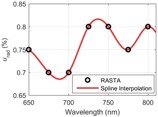
Figure 3.
Radiometric calibration uncertainty of the RAdiometric STAndard (RASTA) [62] and interpolated uncertainties in the simulated sensor.
2.3.4. Temperature-Induced Changes in Photo-Response
The relative radiometric sensitivity to temperature (ℜT) was defined by the linear model coefficients from reference [40]. These coefficients predict a given radiance as a function of temperature, which was assumed to correspond to the detector temperature, Td. ℜT corresponds to the ratio between the radiance predicted radiance at a given temperature to the radiance predicted at a reference temperature. The sensor used in reference [40] was different to the type of sensor simulated in the present study, but also made of Silicon, thus we assumed that it was a suitable approximation representing changes in Silicon photo-response with temperature. These coefficients were interpolated via cubic splines to the spectral bands of the sensor simulator. The characterization dataset was produced by generating radiances between −10 and 40 °C at 10 °C steps from the interpolated coefficients. RASTA spectral radiance was not used in this case, but RASTA uncertainties were added to these radiances as described in Section 2.3.3. These radiances were then processed by the sensor simulator to propagate sensor random noise and radiometric calibration uncertainties. We added also a 2% relative uncertainty to the temperature sensor; which is within the range of uncertainties found in the experiment described in Section 2.3.2. For each temperature level we simulated 30 radiance and Td observations with random normal noise via Monte Carlo sampling. Spectroradiometers one of the type simulated in this work allow setting low detector temperatures (around −10 °C) to reduce noise; therefore we selected −10 °C as a reference temperature (Td,ref) and then modeled ℜT as the relative change in radiance as a function of Td in respect to the radiance observed at Td,ref (and therefore unitless). For each sensor simulator spectral band, a linear model was fitted against ℜT to estimate the fitted sensor model parameters and their uncertainties.
The Fitted Sensor Model predicted ℜT between −10 and 40 °C at 10 °C steps. ℜT predictions and propagated uncertainties were used to bias the vegetation dataset therefore producing the retrieval dataset.
2.3.5. Non-Linearity
A synthetic simulated sensor model representing grey-level related non-linearity (ℜN) [50] was generated using the non-linearity coefficients of a QE Pro spectroradiometer. The characterization dataset was produced from the RASTA radiance spectra. First, the sensor simulator optimized tint at the saturation level (scaled value: 200,000 DN). In the next step, the observations of this radiance were generated as in previous sections, reducing the optimized tint by the following factors: 1.000, 0.975, 0.950, 0.900, 0.850, 0.800, and then up to, 0.100 with 0.100 steps. Thirty realizations with random noise of different uncertainties were produced for each tint. The sensor simulator converted Lλ to Nλ. We then used the simulated sensor model to bias Nλ as a function of the digital value in DN, producing in this way the characterization dataset.
ℜN was calculated as the rate —a variable proportional to Lλ (Equation (3))— normalized by the maximum value of this rate found in each pixel [51]. In order to reduce the effect of noise on the calculation of ℜN, we used the averaged radiance of the 30 samples produced at each tint to compute the maximum rate . Next, a 7th degree polynomial was fitted to predict ℜN as a function of Nscaled; where Nscaled is Nλ – N0,λ scaled after subtracting the mean and dividing by the standard deviation to prevent bad conditioning [63]. Figure 4 shows the simulated and fitted sensor models.
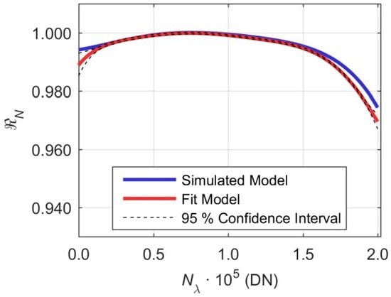
Figure 4.
Simulated and fit non-linearity models.
Once characterized, the fitted sensor model was applied to the vegetation dataset. First, the sensor simulator optimized tint according to L↑app and L↓tot spectra of the vegetation dataset. Then radiances in the vegetation dataset were modified by a factor (fL) of 0.20, 0.40, 0.60, 0.80, 1.00, 1.02, 1.06 and 1.10. Scaled radiances were transferred to the sensor simulator, which, without modifying the value of the optimized tint, transformed Lλ to Nλ. The digital signal Nλ was biased (and noised) by the fitted sensor model and converted back to Lλ units to produce the retrieval dataset.
2.3.6. Directional Response Characterization
The characterized DR of an opaline glass cosine diffuser (Ocean Optics, Dunednin, FL, USA) [53] was used as the base to generate a simulated sensor model. A 4th degree polynomial was fitted for each illumination angle simulated in the experimental data to smooth the response. Cubic spline interpolation was used subsequently to predict the DR at the spectral bands of the simulated sensor at different illumination angles (θs), which became the Simulated Sensor Model (DRsim,λ). A synthetic dataset for the characterization of DR was generated using RASTA radiance for θs equal 0°, 10°, 20°, 30°, 40°, 50°, 60°, 70°, 80° and 85°. An absolute uncertainty of 0.25° was assumed for these angles. For each of them, we produced 30 synthetic radiance spectra including random noise corresponding to lamp, calibration and sensor simulator uncertainties. This was the characterization dataset. Then we computed the relative deviation of irradiance (assuming ) from of the cosine response ( as follows:
where L1,λ and L2,λ represent RASTA radiances at θs = 0° but with different random uncertainties. Figure 5a presents the simulated DR function versus θs at different wavelengths, and compares them with the cosine response. As can be seen, the simulated sensor model overestimates irradiance at short wavelengths and θs; and underestimates it at large θs and wavelengths. Figure 5b shows the relative deviation of the cosine response corresponding to the DR curves in the contiguous subplot. strongly decreases when θs becomes larger than 70°; which is in part explained by the low values of at large angles (Equation (4)). Low values make βλ also very sensitive at to uncertainties at large θs. However, no measurements for SIF retrieval are expected to be reliable at such angles and in the case of the diffuse radiation coming from this angular region, the overall effect is expected to be low since the contribution of diffuse irradiance to the signal is also weighted by (Equation (5)). Fitted sensor model parameters and uncertainties were estimated for each band by fitting a 6th degree polynomial on the characterization dataset, describing as a function of θs.
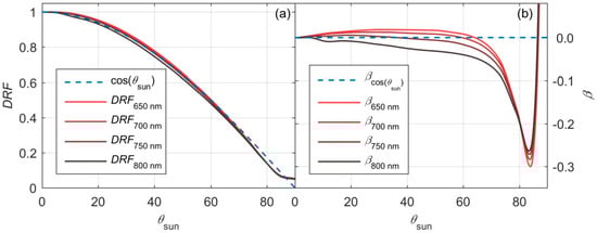
Figure 5.
(a) Cosine diffuser ideal and biased directional responses for different bands. (b) Relative deviation of the cosine response () for the same spectral bands.
The fitted sensor model was used to bias and noise E↓tot in the vegetation dataset using the approach in reference [54]. The vegetation dataset was generated from the Matrix-Operator Model (MOMO) irradiance spectra provided at θs = 0.00°, 2.56°, 16.27°, 29.80°, 43.21°, 56.59°, 69.96° and 83.32°; and L↑app and F↑ were generated as described in Section 2.1. These spectra were convolved with the sensor SRF. Convolved diffuse and direct irradiances were used to calculate the relative direct and diffuse fractions (fdir and fdiff respectively). The surface reflectance factor was not modified in order to isolate the instrumental effect from surface anisotropy. However, F↑ was scaled by the in respect to the signal generated for θs = 29.80° and used in previous analyses: . This normalization is applied to provide an emission approximately proportional to the simulated down-welling irradiance. Consequently, F↑ ranged from 0.45 mW/m2/sr/nm to 0.05 mW/m2/sr/nm in the O2-B band and from 1.61 mW/m2/sr/nm to 0.19 mW/m2/sr/nm in the O2-A band. For each wavelength and solar angle, the fitted sensor model predicted the relative deviation from the cosine response -which was the factor biasing E↓dir-, and the related uncertainties. Similarly, the mean cosine-weighted response error αλ, Equation (5) was computed to bias the diffuse flux, E↓diff, which was always assumed isotropic.
where μs is . E↓tot in the retrieval dataset (E↓tot,DR) was computed as (Equation (6)):
2.4. Uncertainty Estimation and Propagation
Uncertainties in the sensor simulator and the radiance sources were assumed to be uncorrelated and were propagated via a Monte Carlo approach. In order to generate the characterization datasets, we simulated 30 experimental replicates of each observation, adding normal noise to the different quantities or parameters involved in their computation: radiances, radiometric calibration coefficients, dark current, temperature sensors, illumination angle, etc.
Fitted sensor model parameters and related uncertainties were estimated by fitting different models to the characterization datasets. Uncertainties were summarized by the covariance matrix of the parameter estimators (Covp), which was linearly approximated as Equation (7):
where MSE is the Mean Squared Error, J is the Jacobian matrix evaluated at the solution of the model inversion, and superscript T stands for transposed. J is a matrix of n observations and m parameters. Covp allowed uncertainty propagation following the approach in reference [64]. To do so, each time the fitted sensor model was used to predict sensor responses affecting the vegetation dataset, we generated 500 realizations of the model parameters sampling from multivariate normal distributions centered on the parameters values and constrained by Covp. Therefore, the retrieval datasets presented 500 spectra per simulated observation from which F↑ was estimated.
3. Results
3.1. Spectral Calibration Uncertainties
Uncertainties in the location of λc and size of FWHM were 0.59·10−3 nm and 1.34·10−3 nm, respectively. These values describe the incertitude on the determination of these parameters; they do not represent a difference between the nominal and the characterized features or any variation induced by external factors. These uncertainties led to very small errors in the retrieved SIF. In the O2-A band, the Mean Absolute Error (MAE) and Root Mean Squared Error (RMSE) were both 0.003 mW/m2/sr/nm; whereas in the O2-B band MAE and RMSE were 0.008 mW/m2/sr/nm and 0.010 mW/m2/sr/nm, respectively. Absolute errors were always lower than 0.020 mW/m2/sr/nm (95% confidence interval).
Figure 6 shows the difference between F↑ retrieved from the Retrieval Dataset and simulated in the Vegetation Dataset (ΔF↑ = F↑ret - F↑sim) in the two O2 bands. In this case, ΔF↑ represents the retrieval error when one of the up-welling or down-welling fluxes was spectrally shifted in respect to the other. The spectral shifts led to an overestimation of F↑ in the in the O2-B (F687↑) band (Figure 6a) and to under and overestimation of F↑ in the O2-A (F760↑) band (Figure 6b). Errors in F687↑ (ΔF687↑) were above 0.50 mW/m2/sr/nm in most of the cases; and were below this value only when |Δλc| ≤ 0.10 nm, or for large blue shifts in the down-welling flux. Red shifts of the down-welling flux larger than 0.25 nm led to positive errors out of the scale of the plot. Errors in the O2-A band (ΔF760↑, Figure 6b) show F760↑ overestimation for Δλc ≤ −0.25 nm. Larger red shifts (Δλc ≥ 0.25 nm) led to underestimations of lower magnitude. The shortest shifts (|Δλc| ≤ 0.25 nm) led also to |ΔF760↑| < 1.5 mW/m2/sr/nm. The shift of one channel in respect to the other do not produce symmetric errors since O2 features are not symmetric, and due to band selection criteria of the retrieval algorithm.
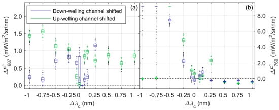
Figure 6.
Estimated minus simulated SIF radiance when the up-welling or the down-welling flux is shifted in (a) the O2-B band and (b) the O2-A band. Notice that in (a), down-welling shifted channel errors for Δλc > 0.25 nm are out of the plot limits.
Figure 7 presents ΔF↑ produced by spectral shifts applied simultaneously to both up and down-welling fluxes. In both cases, deviations from the simulated F↑ were much smaller than in Figure 6. In the O2-B band (Figure 7a), ΔF687↑ reached absolute values below 0.05 mW/m2/sr/nm in the majority of cases. In the O2-A band (Figure 7b), ΔF760↑ was inversely related to Δλc, ranging between −0.20 and 0.07 mW/m2/sr/nm.
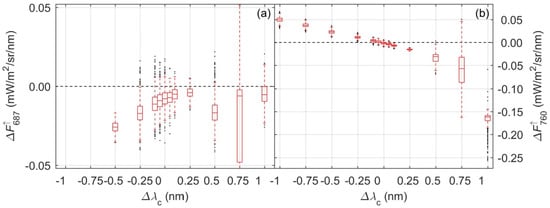
Figure 7.
Estimated minus simulated SIF radiance when both up and down-welling fluxes present the same shift in (a) the O2-B band and (b) the O2-A band.
Table A1 compares the Relative Root Mean Squared Error (RRMSE) induced by spectral shifts in F↑ in the O2-A and O2-B bands as well as on R in two bands located in the red (680 nm) and the near infrared (750 nm) region. These bands were selected because they represent two regions with different R values not affected by changes within the deep and narrow spectral shapes of the O2 features. However, they still provide information about the effect of instrumental artifacts on “traditional” R-based proximal sensing. As can be seen in Table A1, uncertainties and shifts in the spectral features have much stronger effect on F↑ than on R. When the spectral shift was not applied simultaneously to both fluxes, ΔF↑ presented magnitudes comparable to F↑ even for very small Δλc, especially in the O2-B band.
3.2. Temperature-Induced Spectral Changes
Figure 8 shows the results of the characterization of the Tb-induced changes on the spectral features of the system. The interpolated surfaces constitute the fitted sensor model. In order to compute Δλc a Tb = 20 °C was chosen as a reference temperature (Figure 8a). This temperature is close to environmental temperatures used in calibration laboratories. Δλc was weakly dependent on the wavelength, and positively related with Tb. It ranged between −0.078 and 0.120 nm. Therefore, λc red-shifted as its Tb increased. FWHM (Figure 8b) showed a stronger dependency on wavelength, as also observed in [60], however these trends were quite varying. FWHM was positively correlated with Tb at wavelengths below ~670 nm and inversely related with Tb for longer wavelengths.
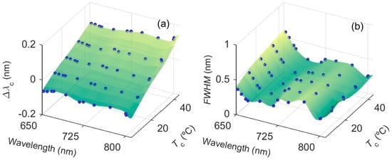
Figure 8.
Chamber temperature effects on (a) the central position of the spectral band and (b) Full Width at Half Maximum. Blue dots represent observations, whereas biharmonic interpolated values are plotted as surfaces.
Figure 9 compares the F↑ retrievals at different Tb vs. the average value retrieved at the reference temperature of 20 °C. Distributions of the errors due to temperature induced changes in the spectral response function are shown in boxes. For comparison, also the errors predicted without uncertainty propagation are presented in circles. In the O2-B band (Figure 9a) Δλc ranged between −0.048 nm and 0.075 nm, and FWHM between 0.234 nm and 0.284 nm. When variations in λc and FWHM were separately applied to each flux measured by the sensor F687↑ was overestimated (Figure 9a), and ΔF687↑ presented wide dispersions with 25th and 75th quartiles between 0.0 and 0.9 mW/m2/sr/nm approximately. In the O2-A band (Figure 9b) spectral features varied more widely than in the O2-B band: Δλc ranged between −0.062 nm and 0.098 nm, and FWHM between 0.434 nm and 0.359 nm. ΔF760↑ presented clear trends with Tb, depending on which flux the spectral changes were applied to. Absolute differences ranged between ~−0.50 mW/m2/sr/nm and ~1.90 mW/m2/sr/nm at the extremes of the range of temperatures tested. In both bands, errors propagated without uncertainties were close to the medians of the distributions. In all cases, ΔF↑ took very low values when variations in the spectral features (FWHM and Δλc) were common to both fluxes.
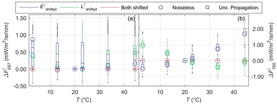
Figure 9.
Chamber temperature effects on spectral features. Estimated fluorescence at different chamber temperatures minus the average SIF radiance at a reference temperature of 20 °C is presented in (a) the O2-B band and (b) the O2-A band. Variations in spectral features are applied to the up-welling, the down-welling or both fluxes. Circles represent the errors in the absence of uncertainties.
Table A2 compares F↑ and the R RRMSE with and without uncertainty propagation. RRMSE are lower and most similar between F↑ and R when the spectral variations equally affect both fluxes. Otherwise there are much larger relative errors in the retrieved F↑. In most of the cases, model uncertainties increased RRMSE.
3.3. Radiometric Calibration Uncertainties
Radiometric calibration uncertainties (only) were propagated to L↑app and L↓tot. In the O2-B band, MAE and RMSE were 0.002 mW/m2/sr/nm and 0.003 mW/m2/sr/nm respectively; the 95% confidence interval (CI) of the errors was [−0.005, 0.007] mW/m2/sr/nm. Analogously, in the O2-A band, MAE and RMSE were 0.001 mW/m2/sr/nm and 0.002 mW/m2/sr/nm respectively; and the 95% CI of the errors was [−0.007, 0.003] mW/m2/sr/nm. In relative terms, these uncertainties translated to a RRMSE of 0.83% and 0.14% for F687↑ and F760↑ respectively, and a RRMSE < 0.01% nearby both O2 bands for R.
3.4. Temperature-Induced Changes in Photo-Response
Figure 10 shows the predicted ℜT used to modify L↑app and L↓tot in the Vegetation Dataset As can be seen, ℜT ~ 0 around 764.4 nm, decreased with increasing Td for shorter wavelengths and increased at higher wavelengths. In the simulated Td range of explored temperatures, average predicted ℜT ranged between 0.996 and 1.000 in the O2-A band, and between 0.954 and 1.000 O2-B band.
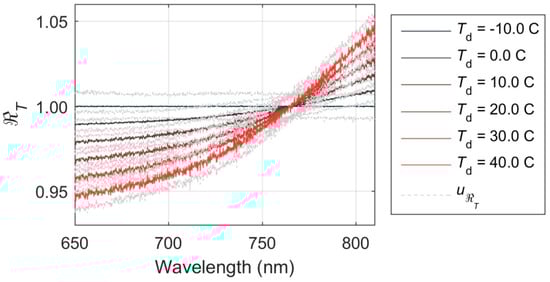
Figure 10.
Simulated radiometric sensitivity to detector temperature with propagated uncertainties.
Figure 11 shows ΔF↑ induced by temperature dependence of detector responsivity, the impact of ℜT was low in both O2 bands. Dispersion induced by propagated uncertainties is presented in boxes. For comparison, the errors induced by the Fitted Sensor Model with no propagation of uncertainties are shown in circles. Median ΔF687↑ (Figure 11a) was inversely related to Td, ranging between 0.00 mW/m2/sr/nm and −0.04 mW/m2/sr/nm, and presented relatively large dispersions. ΔF760↑ was close to 0 in all the cases, but dispersions were larger than in ΔF687↑ (Figure 11b). Errors simulated with no uncertainty propagation were close to median values of the distributions. However, especially in the O2-B band some clear differences could be observed; therefore uncertainties slightly biased the errors in respect to the noiseless predictions of ℜT.
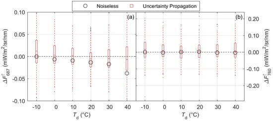
Figure 11.
Detector temperature effects on photo-response. Estimated minus simulated fluorescence radiance in (a) the O2-B band and (b) the O2-A band.
Table A3 presents F↑ and the R RRMSE. For comparison, instrumental-induced errors with and without uncertainty propagation are shown. RRMSE is larger in the O2-B band; and differences between errors in F↑ estimates and the R are lower in the near infrared. Errors induced by noiseless predictions of ℜT suggest that propagated uncertainties seem to be responsible of a large part of the simulated errors.
3.5. Non-Linearity
Figure 12a,b shows ΔF↑ for different radiance scaling factors (fL) applied to the vegetation dataset and biased by fitted sensor model predictions of ℜN in both O2 bands. Distributions generated by the uncertainty propagation are represented in boxes, and errors generated by noiseless predictions of ℜN by circles. Figure 12c,d presents the average predicted ℜN applied inside and outside each of the O2 absorption features. In the O2-B band (Figure 12a,c), the effect of non-linearity was low, and comparable for both the up and the down-welling fluxes inside the band for fL < 0.80. However, for larger fL values, predicted ℜN outside the O2-B band started to decrease for both fluxes, especially after the optimization point (fL = 1.0). The result is an underestimation of F687↑ with ΔF687↑ linearly related with fL for fL ≥ 0.60; saturation level (200,000 DN) was never reached. In the O2-A band (Figure 12b,d) ℜN increased with fL at a similar rate inside and outside the O2 feature up to fL = 0.60. Above this level ℜN saturated close to 1.0 inside the band and decreased up to 0.995 outside the absorption feature. This behavior led to an underestimation of F760↑ with an absolute magnitude ranging between 0.14 mW/m2/sr/nm and 0.31 mW/m2/sr/nm in the fL range [1.00, 1.10]. Errors induced by the noiseless ℜN predictions are in general close to the medians of the distributions generated by uncertainty propagation.
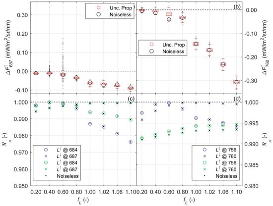
Figure 12.
Non-linearity effects on photo-response. Estimated minus simulated SIF radiance in (a) the O2-B band and (b) the O2-A band. Photo-responsivity applied to the down and the up-welling fluxes inside (x) and outside (o) the (c) O2-B band and (d) the O2-A band.
Table A4 shows the RRMSE in F↑ and R at different fL levels. For comparison, instrument-induced errors with and without uncertainty propagation are presented. Errors in F↑ estimates are large, while they are very low for R in both the red and the near infrared regions. The impact of the propagated uncertainties seems to be low compared with the errors induced by the model. The lowest RRMSE for F↑ seems to be placed close to the optimization point. Relatively larger errors were found for low fL than for fL above optimization. This is in part explained by the reduced magnitude of F↑ (scaled by fL). R in the red spectral region seems to be more affected by ℜN at the bottom of the dynamic range whereas RRMSE is larger at the top of the dynamic range in the near infrared. This is governed by the convolution of spectral radiance and the quantum efficiency of the detector.
3.6. Directional Response of the Cosine Diffuser
Figure 13a,b show the ΔF↑ induced by DR in the O2-B and O2-A bands respectively. For comparison, the F↑ simulated at each band is also presented (stars), as well as the errors induced by the noiseless model (circles). Large differences can be observed between the ΔF↑ generated DR predicted with and without uncertainty propagation. Propagated uncertainties led to much higher errors. In the O2-B band errors are comparable to F687↑ magnitude; whereas in the O2-A band errors are the half the value of F760↑ or less. However, errors induced by the noiseless model are close to 0. The largest errors both in relative and absolute terms are found at the lowest θs.
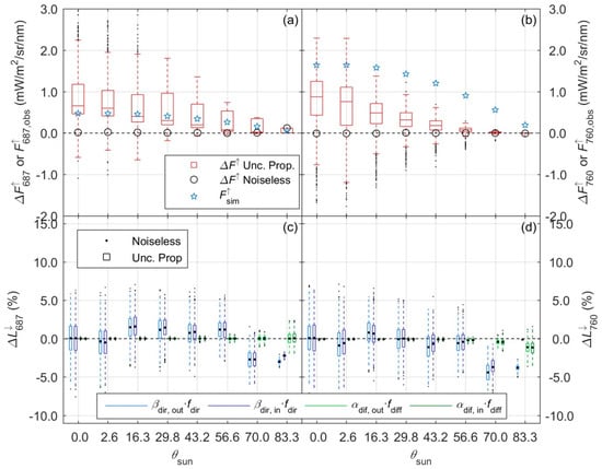
Figure 13.
Cosine diffuser directional response effects. Simulated SIF radiance (stars) at different sun zenith angles and the corresponding error estimated distributions generated by uncertainty propagation (boxes); as well as errors generated by a noiseless the DR model (circles) in (a) the O2-B band and (b) the O2-A band. Variations in radiance induced respect to the ideal cosine response in the diffuse and the direct components of the down-welling flux inside (dark blue/green) and outside (light blue/green) (c) the O2-B band and (d) the O2-A band.
Figure 13c,d show the predictions of the relative variation in L↓tot (ΔL↓,%) induced by the deviations in the measurement of direct (, blue) and the diffuse components (, green) of the down-welling flux in the O2-B and the O2-A bands respectively. For comparison, the distributions generated by the propagation of uncertainties (boxes) as well as those of the noiseless predictions of and (dots) are shown. As can be seen, in this case, medians of the distributions and noiseless values coincide. Variations are presented for radiances inside (dark blue/green) and outside (bright blue/green) of both O2 features. In both cases the direct component of the down-welling flux (direct radiation coming from θs) was more strongly affected by the sensor DR than the diffuse component (assumed isotropic) for θs ≤ 56.6°. Above this angle, the effect of the diffuse component became also relevant since the diffuse fraction increased. However, in most of the cases, ΔL↓ of the direct component presented wider dispersions. ΔL↓ remained below 5% for most of the simulations; ΔL↓ differences between inside and outside the O2 bands were mild, and only noticeable at large θs. However, for θs ≤ 56.6° the median of the distributions and noiseless |ΔL↓| were lower than 1.5% and 0.6% in the O2-B and O2-A bands, respectively.
Predicted DR appears to have a reduced effect on F↑ retrieval; however, the uncertainties associated to the model largely biased F↑ estimates. In this simulation, uncertainty is only propagated to the down-welling radiances involved in the estimation of F↑. Even in absence of DR bias, uncertainties led to F↑ overestimation as shown in Appendix C (Figure A3).
Table A5 compares the RRMSE in F↑ and R for different θs. Instrument-induced errors with and without uncertainty propagation are presented. Errors in F↑ estimates are larger than those found in the reflectance factors, and largely related to the propagated uncertainty. Relative errors in the O2-B and the O2-A band were maximal at the lowest θs tested (~235% and ~65% respectively). In the case of R, RRMSE stay below ~3% for θs <69.96°, most of the error is also induced by the propagated uncertainties. RRMSE achieve also large values at the highest θs, which is expected due to the relatively low signal level.
4. Discussion
This article explores the sensitivity of the retrieval of SIF in the O2-B and O2-A bands to different instrumental biases and noises simulating a state-of-the-art spectroradiometer; and provides a framework to carry out similar analyses that could be relevant for the interpretation and the validation of remote sensing SIF products.
The uncertainties propagated during the simulation of the radiometric and the spectral calibration experiments led to low uncertainties in the respective calibration coefficients; as well as reduced errors in the retrieval of SIF. These results limit to the magnitudes involved in the calibrations, and do not include the analysis of spectral shifts. On the contrary, systematic biases induced by some of the simulated—but realistic—instrumental responses significantly affected SIF retrieval. In this work, the effect of different instrumental responses is analyzed separately. However, in an actual measurement, the total effect on SIF retrieval would depend on several factors including spectral properties of the vegetation target, illumination conditions, sensor characteristics and configuration; the joint effect of different instrumental responses and uncertainties, as well as additional sources of uncertainty that were not analyzed (e.g., solar irradiance stability in the natural environment). Some of the analyses conducted revealed systematic biases and errors related to the factors driving the instrumental responses. This is relevant because some of these factors are also drivers of plant photosynthesis (e.g., solar angle, temperature, radiance level, etc.); and therefore, covariation with errors might spuriously mask or enhance physiologically induced variations of SIF. This might lead to confounding instrumental with vegetation responses to such drivers, and in consequence, to erroneous conclusions and non-repeatable results. The modeling work in this article suggests that instrument characterization is a necessary step in the interpretation of spectroradiometric signals related to plant photosynthesis. The relative errors propagated from the same instrumental responses to red and NIR R were much smaller than those found in SIF. This implies that uncertainty levels that might be acceptable for the calculation of reflectance factors might strongly limit and even invalidate the retrieval of SIF; as well as its use for the study of plant function. Considering the growing interest of the scientific community on SIF, more research is needed to understand the performance of field spectroradiometers and their limitations to provide reliable retrievals of SIF.
Results also indicate that the suitability of current methods and models used to characterize field SIF-oriented spectroradiometers should also be evaluated. As with the spectroradiometric systems, it is also necessary to understand if the characterization methods are good enough; in this case, to predict sensor behaviors and to correct the measurements according to the requirements of the application. For this reason, we propagated sensor model uncertainties to radiances the characterization methods as a way of evaluating if a characterized model could be used to improve SIF retrieval. In some cases, errors were driven by uncertainties propagated from the characterization of the sensor models; which suggests that correction of instrumental biases might be counter-productive if (random) uncertainties were too high to precisely characterize and predict the sensor behavior.
Consequently, more efforts are needed to develop methods and systems that allow the validation or evaluation of SIF retrievals in the field. Some works of this kind have made use of calibrated emission sources, mimicking the F↑ spectrum shape using spherical [65], and panel diffusers (“F-ref” panel, JB Hyperspectral devices); to allow comparing SIF estimates at different radiance emission levels. However, validation of absolute SIF emissions is a complex problem which also depends on the retrieval method [13]. The results presented on this work are limited to a single retrieval algorithm, and may vary for other methods.
4.1. Impact of Spectral Features
These results demonstrate how even very small spectral differences between the measurement of the up and the down-welling fluxes involved in the retrieval of SIF signal can lead to large errors; which can achieve magnitudes comparable or even larger than the actual signal (Figure 6 and Figure 7, Table A1). This makes system design critical. The use of different spectroradiometers to separately measure up-welling and down-welling radiances would be strongly discouraged since: (1) different sensors would never present the same spectral features (e.g., λc, FWHM); and (2) correction would be complex and might involve the use of high spectral resolution atmospheric radiative transfer codes and sensor models that, even then achieving extreme accuracies and precisions, might not be enough to correct SIF retrieval. The final result would strongly depend on the accuracy achieved in the prediction of E↓tot and the stability of the spectral features in each of the sensors.
Thermal stabilization, not only of the detector, but of spectrometer internal and external components of the optical path (spectrometer body, including diffraction grating and mirrors, multiplexers, etc.) is also recommended. Results of Section 3.2 show that if the spectral features equally vary for both the up-welling and the down-welling fluxes, the impact on the retrieval might be very small (Figure 9, Table A2). However, temperature could differently affect the optical path followed by each of the fluxes, which in the worst case scenario would produce spectral shifts in opposite directions, magnifying the errors. The effect of temperature on individual components of the optical path has not been analyzed, and variations observed in Section 3.2 cannot be related or partitioned into any of them. Optical fibers are expected to remain stable at operational temperature ranges of field spectroradiometry [66]. However, to the best of our knowledge, the effect of temperature on different elements of the optical path exposed to environment/not stabilized has not yet been reported in regard to SIF retrieval. This information would be relevant for automated systems operating outdoors to follow daily cycles of SIF, as well as for drones which to date have only afforded the thermal stabilization of the detector, but not of the whole system. The stability of spectral features of sensors operating under dynamic environmental conditions should be quantified through characterization and/or validation. Temperature control and related stability of the spectral features should be coherent both during operation and during the characterization of the systems. Therefore, same temperatures should be used for both types of measurements if possible. In this regard, further analyses are also needed to quantify the uncertainties induced by the different systems that separate the up and down-welling fluxes in their way to the detector.
Mihai et al. [60] compared the performance of line emission lamps and a monochromator to characterize a Piccolo Doppio system featuring a bifurcated optical fiber [26]. After evaluation, they proposed optimizing the spectral characterization in the regions of the O2 spectral bands, where SIF is retrieved. In this sense, the monochromator was preferred to emission line lamps since it could minutely characterize the sensor response in these specific regions; although monochromators also need to be accurately characterized. However, the access to such instrumentation with the spectral resolution reported in that work is not usual in most of the remote sensing laboratories. Nonetheless, the use of different spectral calibration files optimized in each of the bands can be a good alternative to minimize systematic spectral mismatches that might be induced by different system components, if identified.
4.2. Impact of Photo-Response
Instrumental-induced changes in the radiometric response of the sensor also led to lower but still significant errors in the retrieval of SIF. Producers of field spectroradiometers used for the quantification of reflectance factors usually report non-linarites below 1% within the 95% of the radiometric range of the instrument. Though, in some cases, characterization experiments found sensor non-linarites being slightly higher than these 1% [50,53]. In theory, if non-linearity is low for most of the radiometric range of the sensor the most non-linear region can be prevented with an adequate optimization. Still, a correction can be applied based on a polynomial model representing sensor responsivity as a function of the recorded digital signal [51]. Therefore, as long as the correction is accurate, this non-linearity should not pose a critical problem for SIF retrieval. We simulated observations of a sensor not optimizing integration time under varying radiation levels, and SIF relative errors ranged between 10–15% still at the optimization level (Figure 12, Table A4). During the simulation of the non-linearity characterization, we found a misfit between the simulated and the fitted sensor model, which overestimated non-linearity in the extremes of the radiometric range of the sensor (Figure 4). Inaccuracy of the polynomial fit might be in part induced by noise present in the characterization dataset and by the inherent sensitivity of the method to random noise. This is because the highest photo-response used to normalize the rate of DN/ms can often be found in the noisiest measurements [50,51]. A second reason could be the heterogeneous distribution of the data, which prioritizes the fitting in the central region of the radiometric range, but not in the extremes. This should require more careful statistical analysis that the current standard method does not follow. Fitting biases in the extremes of the radiometric range of the detector would be unnoticed provided the actual responsivity is not known, and might increase the errors during SIF retrieval. However, relying only on an adequate optimization of the integration time might not be enough to prevent errors in SIF. In the simulated case, lowest RRMSE, but not the absolute errors, were achieved close to the optimization point (Figure 12, Table A4). This is also a consequence of the varying magnitude of SIF in the simulation. Uncertainties propagated in this exercise had a low impact on SIF, suggesting that in this case, a correction based on the sensor model might increase the accuracy of the retrieval. Further work should be carried out on the characterization of non-linearity in order to improve the methods as well as to test other types of non-linearity not analyzed in this work (e.g., supra-responsivity).
Predicted cosine diffuser DR led to small errors in SIF estimation. However, uncertainties propagated from the fitted sensor model induced much larger errors. The DR of calibrated reference panels was not assessed, but results might be similar to the ones presented in Section 3.6. Uncertainties simulated in the fitted sensor model parameters propagated to outdoors irradiance levels led to noisy spectra, especially at low θs where the irradiance magnitude was large; and consequently large biases on SIF were found in the retrieval. These results are supported by the analysis carried out without propagation of uncertainties (Figure 13c,d), and by the unbiased but noisy simulation presented in Appendix C. These analyses are incomplete since the SIF error will depend on the joint effect of different sensor responses and uncertainties, and the propagation of uncertainties to only one of the fluxes might have inflated the errors in SIF. However, results show that the approach presented can contribute to determining the suitability of a characterized sensor model to correct the measurements. If the uncertainties in the characterized model were too high, the conclusion would be that the characterized DR model could not be applied to correct the down-welling irradiance. Nonetheless, even if possible, the correction of DR is especially challenging due to unknown directional distribution of the diffuse irradiance. The measurement of such distribution would be complex [67] and maybe not accurate enough for the application. Alternatively, diffuse irradiance could be assumed isotropic and estimated inverting atmospheric radiative transfer codes from the observed down-welling irradiance [68]. Furthermore, the consequences of such an assumption on the retrieval of SIF are still not well understood. In practice, diffusers and panels featuring DR close enough to the cosine response would be preferable if this allowed avoiding any correction; however this point remains to be validated. DR characterization and the framework of uncertainty propagation provided in this article might also help to stablish θs and diffuse fraction thresholds above which SIF retrievals cannot be trusted. The fraction of diffuse irradiance is usually low in remote sensing applications (cloudy data are discarded), but can be large in the case of automated proximal sensing [36]. Another challenge related with the DR is the adequate leveling of diffusers and panels, which is especially relevant for drones, but also for tower-based systems and hand held operations.
In this article, we also analyzed the thermal-induced changes in detector responsivity. Since the system we simulated used the same sensor to measure both the up-welling and the down-welling fluxes, the impact on SIF retrieval was low and led to noise rather than biases (Figure 10 or Table A3). In fact, in the O2-B band these biases resulted in average reduced by the noise. In a situation of detector temperature variation, most of the error induced on SIF could be due to changes in the spectral response functions. However, temperature responsivity would be a factor to consider if two different sensors were employed to sample each of the fluxes involved in the computation of SIF, which is already discouraged. Still, in such a situation the spectral differences between detectors would be far more important.
5. Conclusions
This work analyzed the effect of different instrumental responses on the retrieval of sun-induced chlorophyll fluorescence. The analysis is limited to some specific cases, but provides a framework that can be used in the future to carry out similar assessments, which are needed to understand the reliability of proximal sensing-based SIF retrievals. Results show that certain instrumental responses can have a minor or negligible effect on reflectance factors, while strongly affecting the retrieval of SIF. In other cases, sensor responses had little effect on SIF, but large errors were induced by sensor model propagated uncertainties. This suggests that field spectroradiometry dedicated to the observation of passive SIF could require new and higher quality standards than those in use for the quantification of reflectance factors; as well as more accurate characterization of the sensors, and propagation of uncertainties. The growing interest in proximal sensing of SIF contrasts with the seemingly minimal work carried out in this regard. The main risk is the existence of common drivers of the instrumental responses and vegetation physiology, the ultimate target of SIF retrieval from remotely sensed data. Adequate calibration, characterization and understanding of sensor responses are crucial to prevent spurious results and erroneous conclusions, as well as to ensure the quality of ground measurements dedicated to the validation and scaling of SIF. Also, comparisons of calibration standards used or standardization of calibration procedures and facilities should be evaluated. These activities are key factors to support, evaluate and validate retrievals carried out from airborne and satellite-borne sensors, such as the up-coming mission FLEX; as well as to understand the relationships between SIF and plant physiology. Some of the instrumental responses analyzed here can be partially controlled by spectroradiometer and system design; however, we still need to define how good is good enough. The range of conditions within which the retrieval of SIF is viable is not well understood, and depends in parts on the system as well as on the retrieval methods. In addition, the suitability of characterization and correction methods as well as the effect of other instrumental responses not considered in this work, such as etaloning [26], should be evaluated.
Author Contributions
J.P.-L., A.H., and L.M. designed this study; J.P.-L., T.J., K.S., L.A., A.M.A., L.M., A.H. and A.B. produced or provided data; J.P.-L. designed the methodology, carried out the analyses and prepared the draft; A.H., A.M.A., D.S., L.M., J.K., K.S., Y.G., M.P.C.-M. and H.A. reviewed and edited the manuscript; A.M.A. was in charge of validation; J.P.-L., M.P.C.-M., H.A. and A.M.A. supervised this article.
Funding
This publication is based upon work from COST Action ES1309 OPTIMISE, supported by COST (European Cooperation in Science and Technology; www.cost.eu). Mac Arthur, A. was funded during COST Action ES1309 by the UK’s NERC/NCEO Field Spectroscopy Facility at the School of GeoSciences, University of Edinburgh. Sporea, D. and Mihai, L. acknowledge the financial support of the Romanian Space Agency under the contract STAR 131/2017. This project has received funding from the European Union’s Horizon 2020 research and innovation programme under the Marie Skłodowska-Curie grant agreement No 749323 (https://ec.europa.eu/research/mariecurieactions/), held by Sakowska, K. Cendrero-Mateo, M.P. and Alonso, L. were funded by AVANFLEX project (Advanced Products for the FLEX mission), n° ESP2016-79503-C2-1-P, Ministry of Economy and Competitiveness, Spain. The contributions by Hueni, A. were supported by the University of Zurich Priority Programme on Global Change and Biodiversity (URPP GCB) and by the MetEOC project in the frameworks of EMRP and EMPIR supported by the European Union. Pacheco-Labrador, J. was supported by the EnMAP project MoReDEHESHyReS “Modelling Responses of Dehesas with Hyperspectral Remote Sensing” (Contract No. 50EE1621, German Aerospace Center (DLR) and the German Federal Ministry of Economic Affairs and Energy) and the German Federal Ministry of Economic Affairs and Energy) and the Alexander von Humboldt Foundation via Max-Planck Prize to Markus Reichstein.
Acknowledgments
Authors are grateful to the COST Action ES1309 “Innovative optical Tools for proximal sensing of ecophysiological processes” (OPTIMISE) for their primacy in facilitating the scientific networking that resulted in this work. We are also grateful to FLUSS project (Atmospheric Corrections for Fluorescence Signal and Surface Pressure Retrieval over Land) and the Freie Universität Berlin for providing the very high spectral resolution dataset generated with MOMO. We also acknowledge COST Action CA17134 “Optical synergies for spatiotemporal SENsing of Scalable ECOphysiological traits” (SENSECO) for its support on networking and dissemination.
Conflicts of Interest
The authors declare no conflict of interest.
Appendix A. Sensor Simulator
The Sensor Simulator operation is summarized in Figure A1. In this appendix, we use σ to symbolize the standard deviation of any of the distributions represented.

Figure A1.
Scheme of operation of the sensor simulator.
An “observed” radiance is characterized by a distribution of radiances () representing with a given mean (), and some random noise of standard deviation σ. can be produced either by spectral convolution of the very high spectral resolution radiances () generated as described in Section 2.1 or by interpolation of the RASTA radiance with some associated uncertainties to the spectral features of the sensor simulator. Spectral convolution is done using distributions of the sensor central wavelength and full-width at half maximum .
is used to optimize the integration time (tint) according to and the radiometric calibration coefficients () and the associated uncertainties (). tint is optimized so that the signal reaches 175,000 digital numbers (DN), which represents the 85% of the sensor simulator saturation value. tint and are then transferred to the noise generator, which produces random noise as a function of both. The radiometric calibration coefficients are used to digitize the radiances to digital number units a certain distribution of dark current . Dark current is supposed to be known since can be measured after optimization. At this stage, is added to the digital signal distribution . Finally, is added to the digital signal, removed from it, and the outgoing distribution of radiances generated using in this case both and the associated uncertainties ().
For the noise generator, we used data from the signal-to-noise ratio (SNR) characterization of a QE Pro spectroradiometer and fit a predictive model as a function of tint and of the rate -a variable proportional to Lλ. Figure A2 represents this dataset and the fitted plane which is used by the sensor simulator to estimate the level of noise .

Figure A2.
Signal-to-Noise as a function of integration time and the ratio of digital signal to integration time and the plane fit to observations.
Appendix B. F↑ and R Relative Root Mean Squared Errors Comparison

Table A1.
Relative Root Mean Squared Error (%) induced by spectral uncertainties on F↑ and R.
Table A1.
Relative Root Mean Squared Error (%) induced by spectral uncertainties on F↑ and R.
| Δλc (nm) | −1.00 | −0.75 | −0.50 | −0.25 | −0.10 | −0.05 | 0.0 | 0.05 | 0.10 | 0.25 | 0.50 | 0.75 | 1.00 |
|---|---|---|---|---|---|---|---|---|---|---|---|---|---|
| Spectral shift in Both Fluxes | |||||||||||||
| F687↑ | 224.1 | 225.2 | 65.5 | 4.5 | 3.2 | 2.8 | 2.3 | 2.1 | 1.7 | 1.3 | 4.5 | 8.8 | 2.2 |
| F760↑ | 3.5 | 2.6 | 1.6 | 0.8 | 0.4 | 0.2 | 0.2 | 0.3 | 0.5 | 1.1 | 2.5 | 5.1 | 11.8 |
| R680 | 0.6 | 0.4 | 0.3 | 0.2 | 0.1 | 0.0 | 0.0 | 0.0 | 0.1 | 0.2 | 0.3 | 0.5 | 0.7 |
| R750 | 0.8 | 0.6 | 0.4 | 0.2 | 0.1 | 0.0 | 0.0 | 0.0 | 0.1 | 0.2 | 0.4 | 0.6 | 0.8 |
| Spectral shift in the up-welling flux | |||||||||||||
| F687↑ | 347.9 | 379.7 | 275.4 | 252.5 | 66.5 | 17.8 | 2.3 | 200.9 | 234.8 | 175.5 | 212.1 | 158.0 | 209.0 |
| F760↑ | 4.1 | 5.8 | 641.8 | 341.3 | 75.9 | 46.0 | 0.2 | 12.2 | 28.4 | 162.6 | 32.4 | 44.1 | 33.0 |
| R680 | 0.6 | 0.4 | 0.3 | 0.1 | 0.1 | 0.0 | 0.0 | 0.0 | 0.1 | 0.2 | 0.3 | 0.5 | 0.7 |
| R750 | 0.8 | 0.6 | 0.4 | 0.2 | 0.1 | 0.1 | 0.0 | 0.0 | 0.1 | 0.2 | 0.3 | 0.5 | 0.8 |
| Spectral Shift in the down-welling flux | |||||||||||||
| F687↑ | 61.2 | 46.4 | 175.9 | 203.1 | 161.4 | 137.8 | 2.3 | 41.6 | 62.8 | 282.1 | 661.0 | 955.3 | 973.6 |
| F760↑ | 639.5 | 631.3 | 519.5 | 159.2 | 19.2 | 20.2 | 0.2 | 30.9 | 60.5 | 17.2 | 25.5 | 15.9 | 27.7 |
| R680 | 0.0 | 0.0 | 0.0 | 0.0 | 0.0 | 0.0 | 0.0 | 0.0 | 0.0 | 0.0 | 0.0 | 0.0 | 0.0 |
| R750 | 0.0 | 0.0 | 0.0 | 0.0 | 0.0 | 0.0 | 0.0 | 0.0 | 0.0 | 0.0 | 0.0 | 0.0 | 0.0 |
Table A2.
Relative Root Mean Squared Error (%) induced by spectral variations induced by chamber temperature on F↑ and R accounting for uncertainty propagation (U) and ignoring it (Ø).
Table A2.
Relative Root Mean Squared Error (%) induced by spectral variations induced by chamber temperature on F↑ and R accounting for uncertainty propagation (U) and ignoring it (Ø).
| Tb (°C) | 2.9 | 12.9 | 20.0 | 23.1 | 33.4 | 44.4 |
|---|---|---|---|---|---|---|
| Spectral shift in Both Fluxes | ||||||
| F687↑ (U) | 1.88 | 1.33 | 1.27 | 1.20 | 1.22 | 1.28 |
| F760↑ (U) | 0.26 | 0.21 | 0.23 | 0.22 | 0.29 | 0.44 |
| F687↑ (Ø) | 1.62 | 0.26 | 0.00 | 0.30 | 0.90 | 0.80 |
| F760↑ (Ø) | 0.37 | 0.09 | 0.00 | 0.03 | 0.08 | 0.41 |
| R680 (U) | 0.03 | 0.02 | 0.01 | 0.01 | 0.02 | 0.05 |
| R750 (U) | 0.05 | 0.03 | 0.01 | 0.01 | 0.04 | 0.08 |
| R680 (Ø) | 0.03 | 0.01 | 0.00 | 0.00 | 0.02 | 0.05 |
| R750 (Ø) | 0.05 | 0.02 | 0.00 | 0.01 | 0.04 | 0.08 |
| Spectral shift in the up-welling flux | ||||||
| F687↑ (U) | 139.30 | 121.39 | 1.27 | 119.50 | 106.25 | 150.48 |
| F760↑ (U) | 76.35 | 38.86 | 0.23 | 19.17 | 29.11 | 22.86 |
| F687↑ (Ø) | 93.26 | 15.72 | 0.01 | 0.99 | 25.83 | 114.23 |
| F760↑ (Ø) | 65.06 | 31.06 | 0.14 | 8.79 | 28.85 | 5.56 |
| R680 (U) | 0.04 | 0.02 | 0.01 | 0.01 | 0.02 | 0.05 |
| R750 (U) | 0.06 | 0.03 | 0.01 | 0.01 | 0.04 | 0.08 |
| R680 (Ø) | 0.03 | 0.01 | 0.00 | 0.00 | 0.02 | 0.05 |
| R750 (Ø) | 0.05 | 0.02 | 0.00 | 0.01 | 0.04 | 0.08 |
| Spectral Shift in the down-welling flux | ||||||
| F687↑ (U) | 157.90 | 131.67 | 1.27 | 135.40 | 139.61 | 138.17 |
| F760↑ (U) | 31.32 | 23.25 | 0.23 | 24.62 | 62.39 | 128.10 |
| F687↑ (Ø) | 208.34 | 7.61 | 0.00 | 0.53 | 5.18 | 35.95 |
| F760↑ (Ø) | 35.92 | 17.24 | 0.00 | 9.63 | 51.45 | 116.05 |
| R680 (U) | 0.01 | 0.01 | 0.01 | 0.01 | 0.00 | 0.00 |
| R750 (U) | 0.00 | 0.00 | 0.00 | 0.00 | 0.00 | 0.00 |
| R680 (Ø) | 0.03 | 0.01 | 0.00 | 0.00 | 0.02 | 0.05 |
| R750 (Ø) | 0.05 | 0.02 | 0.00 | 0.01 | 0.04 | 0.08 |
Table A3.
Relative Root Mean Squared Error (%) induced by photo-response variations induced by sensor temperature on F↑ and R accounting for uncertainty propagation (U) and ignoring it (Ø).
Table A3.
Relative Root Mean Squared Error (%) induced by photo-response variations induced by sensor temperature on F↑ and R accounting for uncertainty propagation (U) and ignoring it (Ø).
| Td (°C) | −10.0 | 0.0 | 10.0 | 20.0 | 30.0 | 40.0 |
|---|---|---|---|---|---|---|
| F687↑ (U) | 65.34 | 48.72 | 50.10 | 35.36 | 57.88 | 70.80 |
| F760↑ (U) | 4.54 | 3.66 | 3.61 | 3.71 | 3.78 | 4.22 |
| F687↑ (Ø) | 0.00 | 1.60 | 2.26 | 3.28 | 4.11 | 9.20 |
| F760↑ (Ø) | 0.00 | 0.19 | 0.06 | 0.20 | 0.23 | 0.24 |
| R680 (U) | 0.52 | 0.46 | 0.44 | 0.42 | 0.47 | 0.56 |
| R750 (U) | 0.57 | 0.51 | 0.46 | 0.43 | 0.52 | 0.55 |
| R680 (Ø) | 0.00 | 0.00 | 0.00 | 0.00 | 0.00 | 0.00 |
| R750 (Ø) | 0.00 | 0.00 | 0.00 | 0.00 | 0.00 | 0.00 |
Table A4.
Relative Root Mean Squared Error (%) induced by non-linearity on F↑ and R accounting for uncertainty propagation (U) and ignoring it (Ø).
Table A4.
Relative Root Mean Squared Error (%) induced by non-linearity on F↑ and R accounting for uncertainty propagation (U) and ignoring it (Ø).
| fL (-) | 0.20 | 0.40 | 0.60 | 0.80 | 1.00 | 1.02 | 1.06 | 1.10 |
|---|---|---|---|---|---|---|---|---|
| F687↑ (U) | 82.59 | 62.52 | 43.18 | 29.00 | 15.66 | 14.59 | 13.11 | 12.36 |
| F760↑ (U) | 80.14 | 60.33 | 41.24 | 22.27 | 10.20 | 10.02 | 10.27 | 11.53 |
| F687↑ (Ø) | 82.79 | 62.96 | 44.63 | 28.40 | 14.74 | 15.93 | 11.42 | 11.20 |
| F760↑ (Ø) | 80.25 | 60.89 | 42.88 | 22.34 | 10.11 | 9.99 | 10.28 | 11.56 |
| R680 (U) | 1.65 | 1.22 | 0.98 | 0.71 | 0.38 | 0.34 | 0.25 | 0.15 |
| R750 (U) | 0.07 | 0.04 | 0.08 | 0.19 | 0.80 | 0.93 | 1.23 | 1.57 |
| R680 (Ø) | 1.62 | 1.19 | 0.97 | 0.69 | 0.38 | 0.34 | 0.25 | 0.15 |
| R750 (Ø) | 0.06 | 0.03 | 0.08 | 0.19 | 0.80 | 0.93 | 1.23 | 1.58 |
Table A5.
Relative Root Mean Squared Error (%) induced by the diffuser directional response on F↑ and R for uncertainty propagation (U) and ignoring it (Ø).
Table A5.
Relative Root Mean Squared Error (%) induced by the diffuser directional response on F↑ and R for uncertainty propagation (U) and ignoring it (Ø).
| θs (°) | 0.00 | 2.56 | 16.27 | 29.80 | 43.21 | 56.59 | 69.96 | 83.32 |
|---|---|---|---|---|---|---|---|---|
| F687↑ (U) | 234.75 | 214.63 | 186.95 | 174.51 | 152.60 | 132.46 | 140.06 | 185.68 |
| F760↑ (U) | 64.91 | 58.13 | 40.55 | 29.87 | 22.30 | 13.78 | 8.40 | 2.79 |
| F687↑ (Ø) | 3.25 | 4.83 | 2.87 | 1.32 | 1.07 | 1.06 | 2.32 | 214.71 |
| F760↑ (Ø) | 0.64 | 0.61 | 0.72 | 0.56 | 0.20 | 0.01 | 0.51 | 2.86 |
| R680 (U) | 2.31 | 2.11 | 2.52 | 1.88 | 1.67 | 1.97 | 8.46 | 10.20 |
| R750 (U) | 2.38 | 2.20 | 2.21 | 1.73 | 2.30 | 2.54 | 8.21 | 9.62 |
| R680 (Ø) | 0.69 | 0.25 | 1.77 | 1.04 | 0.12 | 1.28 | 8.27 | 10.15 |
| R750 (Ø) | 0.35 | 0.55 | 1.07 | 0.08 | 1.42 | 1.97 | 8.01 | 9.60 |
Appendix C. Effect of Propagated Uncertainties on F Retrieval in the DR Model
Result suggested that uncertainties in the parameters of the fitted sensor model representing the cosine diffuser DR had a strong impact on SIF retrieval, leading mainly to overestimation. To test this effect, we simulated uncertainties of similar range than the ones propagated to the L↓tot at θs = 0°. This was achieved sampling noise from a normal distribution of mean 0 and 3.5 times the standard deviation of the simulated L↓tot. This standard deviation was calculated at each band and had to be scaled by a factor of 3.5 since the final uncertainties did not follow aF normal distribution. Then noise samples of size n = 50 were add to L↓tot (not affected by cosine DR) multiplied by a scaling factor fσ ranging between 0.0 and 1.0 with 0.1 steps. Figure A3a,b shows the error in the estimation of F↑ in the O2-B and O2-A bands respectively. As can be seen, errors increase with fσ reaching levels similar to those shown in Figure 13a,b for θs = 0° when fσ ~ 1.0.

Figure A3.
Effect DR Fit Model uncertainty propagation on the retrieval of F in (a) the O2-B band and (b) the O2-A band as a function of the scaling factor fσ.
References
- Meroni, M.; Rossini, M.; Guanter, L.; Alonso, L.; Rascher, U.; Colombo, R.; Moreno, J. Remote sensing of solar-induced chlorophyll fluorescence: Review of methods and applications. Remote Sens. Environ. 2009, 113, 2037–2051. [Google Scholar] [CrossRef]
- Frankenberg, C.; Berry, J. 3.10-Solar Induced Chlorophyll Fluorescence: Origins, Relation to Photosynthesis and Retrieval. In Comprehensive Remote Sensing; Liang, S., Ed.; Elsevier: Oxford, UK, 2018; pp. 143–162. [Google Scholar]
- Frankenberg, C.; Fisher, J.B.; Worden, J.; Badgley, G.; Saatchi, S.S.; Lee, J.-E.; Toon, G.C.; Butz, A.; Jung, M.; Kuze, A.; et al. New global observations of the terrestrial carbon cycle from GOSAT: Patterns of plant fluorescence with gross primary productivity. Geophys. Res. Lett. 2011, 38. [Google Scholar] [CrossRef]
- Guanter, L.; Frankenberg, C.; Dudhia, A.; Lewis, P.E.; Gómez-Dans, J.; Kuze, A.; Suto, H.; Grainger, R.G. Retrieval and global assessment of terrestrial chlorophyll fluorescence from GOSAT space measurements. Remote Sens. Environ. 2012, 121, 236–251. [Google Scholar] [CrossRef]
- Joiner, J.; Guanter, L.; Lindstrot, R.; Voigt, M.; Vasilkov, A.P.; Middleton, E.M.; Huemmrich, K.F.; Yoshida, Y.; Frankenberg, C. Global monitoring of terrestrial chlorophyll fluorescence from moderate-spectral-resolution near-infrared satellite measurements: Methodology, simulations, and application to GOME-2. Atmos. Meas. Tech. 2013, 6, 2803–2823. [Google Scholar] [CrossRef]
- ESA. Report for Mission Selection: FLEX; ESA: Noordwijk, The Netherlands, 2015. [Google Scholar]
- Moreno, J.F.; Asner, G.P.; Bach, H.; Belenguer, T.; Bell, A.; Buschmann, C.; Calera, A.; Calpe, J.; Campbell, P.; Cecchi, G.; et al. Fluorescence Explorer (FLEX): An Optimised Payload to Map Vegetation Photosynthesis from Space; AIAA: Valencia, Spain, 2006. [Google Scholar]
- Rossini, M.; Nedbal, L.; Guanter, L.; Ač, A.; Alonso, L.; Burkart, A.; Cogliati, S.; Colombo, R.; Damm, A.; Drusch, M.; et al. Red and far red Sun-induced chlorophyll fluorescence as a measure of plant photosynthesis. Geophys. Res. Lett. 2015, 42, 1632–1639. [Google Scholar] [CrossRef]
- Ač, A.; Malenovský, Z.; Olejníčková, J.; Gallé, A.; Rascher, U.; Mohammed, G. Meta-analysis assessing potential of steady-state chlorophyll fluorescence for remote sensing detection of plant water, temperature and nitrogen stress. Remote Sens. Environ. 2015, 168, 420–436. [Google Scholar] [CrossRef]
- Celesti, M.; van der Tol, C.; Cogliati, S.; Panigada, C.; Yang, P.; Pinto, F.; Rascher, U.; Miglietta, F.; Colombo, R.; Rossini, M. Exploring the physiological information of Sun-induced chlorophyll fluorescence through radiative transfer model inversion. Remote Sens. Environ. 2018, 215, 97–108. [Google Scholar] [CrossRef]
- Plascyk, J.A. The MK II Fraunhofer Line Discriminator (FLD-II) for Airborne and Orbital Remote Sensing of Solar-Stimulated Luminescence. OPTICE 1975, 14, 144339. [Google Scholar] [CrossRef]
- Aasen, H.; Van Wittenberghe, S.; Sabater, N.; Damm, A.; Goulas, Y.; Wieneke, S.; Hueni, A.; Malenovský, Z.; Alonso, L.; Pacheco-Labrador, J.; et al. Sun-induced chlorophyll fluorescence II: Review of passive measurement setups, protocols and their application at leaf to canopy scale. Remote Sens. 2019, 11, 927. [Google Scholar] [CrossRef]
- Cendrero-Mateo, M.P.; Wieneke, S.; Damm, A.; Pinto, F.; Moreno, J.; Alonso, L.; Guanter, L.; Celesti, M.; Sabater, N.; Cogliati, S.; et al. Sun-induced chlorophyll fluorescence III: Benchmarking retrieval methods and sensor characteristics for proximal sensing. Remote Sens. 2019, 11, 962. [Google Scholar]
- Gamon, J.A.; Peñuelas, J.; Field, C.B. A narrow-waveband spectral index that tracks diurnal changes in photosynthetic efficiency. Remote Sens. Environ. 1992, 41, 35–44. [Google Scholar] [CrossRef]
- Daumard, F.; Goulas, Y.; Ounis, A.; Pedrós, R.; Moya, I. Measurement and correction of atmospheric effects at different altitudes for remote sensing of sun-induced fluorescence in oxygen absorption bands. IEEE Trans. Geosci. Remote Sens. 2015, 53, 5180–5196. [Google Scholar] [CrossRef]
- Meroni, M.; Barducci, A.; Cogliati, S.; Castagnoli, F.; Rossini, M.; Busetto, L.; Migliavacca, M.; Cremonese, E.; Galvagno, M.; Colombo, R.; et al. The hyperspectral irradiometer, a new instrument for long-term and unattended field spectroscopy measurements. Rev. Sci. Instrum. 2011, 82, 043106. [Google Scholar] [CrossRef] [PubMed]
- Cogliati, S.; Rossini, M.; Julitta, T.; Meroni, M.; Schickling, A.; Burkart, A.; Pinto, F.; Rascher, U.; Colombo, R. Continuous and long-term measurements of reflectance and sun-induced chlorophyll fluorescence by using novel automated field spectroscopy systems. Remote Sens. Environ. 2015, 164, 270–281. [Google Scholar] [CrossRef]
- Perez-Priego, O.; Guan, J.; Rossini, M.; Fava, F.; Wutzler, T.; Moreno, G.; Carvalhais, N.; Carrara, A.; Kolle, O.; Julitta, T.; et al. Sun-induced chlorophyll fluorescence and photochemical reflectance index improve remote-sensing gross primary production estimates under varying nutrient availability in a typical Mediterranean savanna ecosystem. Biogeosciences 2015, 12, 6351–6367. [Google Scholar] [CrossRef]
- Liu, L.; Liu, X.; Hu, J.; Guan, L. Assessing the wavelength-dependent ability of solar-induced chlorophyll fluorescence to estimate the GPP of winter wheat at the canopy level. Int. J. Remote Sens. 2017, 38, 4396–4417. [Google Scholar] [CrossRef]
- Daumard, F.; Goulas, Y.; Champagne, S.; Fournier, A.; Ounis, A.; Olioso, A.; Moya, I. Continuous Monitoring of Canopy Level Sun-Induced Chlorophyll Fluorescence During the Growth of a Sorghum Field. IEEE Trans. Geosci. Remote Sens. 2012, 50, 4292–4300. [Google Scholar] [CrossRef]
- Daumard, F.; Champagne, S.; Fournier, A.; Goulas, Y.; Ounis, A.; Hanocq, J.F.; Moya, I. A Field Platform for Continuous Measurement of Canopy Fluorescence. IEEE Trans. Geosci. Remote Sens. 2010, 48, 3358–3368. [Google Scholar] [CrossRef]
- Goulas, Y.; Fournier, A.; Daumard, F.; Champagne, S.; Ounis, A.; Marloie, O.; Moya, I. Gross Primary Production of a Wheat Canopy Relates Stronger to Far Red Than to Red Solar-Induced Chlorophyll Fluorescence. Remote Sens. 2017, 9, 97. [Google Scholar] [CrossRef]
- Guanter, L.; Rossini, M.; Colombo, R.; Meroni, M.; Frankenberg, C.; Lee, J.-E.; Joiner, J. Using field spectroscopy to assess the potential of statistical approaches for the retrieval of sun-induced chlorophyll fluorescence from ground and space. Remote Sens. Environ. 2013, 133, 52–61. [Google Scholar] [CrossRef]
- Cheng, Y.-B.; Middleton, E.; Zhang, Q.; Huemmrich, K.; Campbell, P.; Corp, L.; Cook, B.; Kustas, W.; Daughtry, C. Integrating Solar Induced Fluorescence and the Photochemical Reflectance Index for Estimating Gross Primary Production in a Cornfield. Remote Sens. 2013, 5, 6857. [Google Scholar] [CrossRef]
- Julitta, T.; Corp, L.; Rossini, M.; Burkart, A.; Cogliati, S.; Davies, N.; Hom, M.; Mac Arthur, A.; Middleton, E.; Rascher, U.; et al. Comparison of Sun-Induced Chlorophyll Fluorescence Estimates Obtained from Four Portable Field Spectroradiometers. Remote Sens. 2016, 8, 122. [Google Scholar] [CrossRef]
- Mac Arthur, A.; Robinson, I.; Rossini, M.; Davis, N.; MacDonald, K. A dual-field-of-view spectrometer system for reflectance and fluorescence measurements (Piccolo Doppio) and correction of etaloning. In Proceedings of the 5th International Workshop on Remote Sensing of Vegetation Fluorescence, Paris, France, 22–24 April 2014. [Google Scholar]
- Zhou, X.; Liu, Z.; Xu, S.; Zhang, W.; Wu, J. An Automated Comparative Observation System for Sun-Induced Chlorophyll Fluorescence of Vegetation Canopies. Sensors 2016, 16, 775. [Google Scholar] [CrossRef]
- Yang, K.; Ryu, Y.; Dechant, B.; Berry, J.A.; Hwang, Y.; Jiang, C.; Kang, M.; Kim, J.; Kimm, H.; Kornfeld, A.; et al. Sun-induced chlorophyll fluorescence is more strongly related to absorbed light than to photosynthesis at half-hourly resolution in a rice paddy. Remote Sens. Environ. 2018, 216, 658–673. [Google Scholar] [CrossRef]
- Grossmann, K.; Frankenberg, C.; Magney, T.S.; Hurlock, S.C.; Seibt, U.; Stutz, J. PhotoSpec: A new instrument to measure spatially distributed red and far-red Solar-Induced Chlorophyll Fluorescence. Remote Sens. Environ. 2018, 216, 311–327. [Google Scholar] [CrossRef]
- Hu, J.; Liu, X.; Liu, L.; Guan, L. Evaluating the Performance of the SCOPE Model in Simulating Canopy Solar-Induced Chlorophyll Fluorescence. Remote Sens. 2018, 10, 250. [Google Scholar] [CrossRef]
- Rossini, M.; Meroni, M.; Celesti, M.; Cogliati, S.; Julitta, T.; Panigada, C.; Rascher, U.; van der Tol, C.; Colombo, R. Analysis of red and far-red sun-induced chlorophyll fluorescence and their ratio in different canopies based on observed and modeled data. Remote Sens. 2016, 8, 412. [Google Scholar] [CrossRef]
- Jones, H.G.; Vaughan, R.A. Remote Sensing of Vegetation: Principles, Techniques, and Applications; Oxford University Press: Oxford, UK; New York, NY, USA, 2010. [Google Scholar]
- JCGM. International Vocabulary of Metrology—Basic and General Concepts and Associated Terms (VIM) 3rd edition (2008 version with minor corrections); © JCGM 2012. Available online: http://www.iso.org/sites/JCGM/VIM-JCGM200.htm (accessed on 19 April 2019).
- Damm, A.; Erler, A.; Hillen, W.; Meroni, M.; Schaepman, M.E.; Verhoef, W.; Rascher, U. Modeling the impact of spectral sensor configurations on the FLD retrieval accuracy of sun-induced chlorophyll fluorescence. Remote Sens. Environ. 2011, 115, 1882–1892. [Google Scholar] [CrossRef]
- Wang, H.; Song, H.; Chen, Y.; Laney, S.R. Correcting temperature dependence in miniature spectrometers used in cold polar environments. Appl. Opt. 2015, 54, 3162–3172. [Google Scholar] [CrossRef]
- Pacheco-Labrador, J.; Martín, M. Characterization of a Field Spectroradiometer for Unattended Vegetation Monitoring. Key Sensor Models and Impacts on Reflectance. Sensors 2015, 15, 4154–4175. [Google Scholar] [CrossRef] [PubMed]
- Saber, G.R.S.; Fox, N.P.; Theocharous, E.; Sun, T.; Grattan, K.T.V. Temperature and nonlinearity corrections for a photodiode array spectrometer used in the field. Appl. Opt. 2011, 50, 866–875. [Google Scholar]
- Achatzi, J.; Fischer, G.; Zimmer, V.; Paulus, D. Estimating an Image Sensor’s Temperature for Darksignal-Correction; SPIE: Bellingham, WA, USA, 2014; Volume 9022. [Google Scholar]
- Wang, H.; Chen, Y.; Song, H.; Laney, S.R. A fiber optic spectrometry system for measuring irradiance distributions in sea ice environments. J. Atmos. Ocean. Technol. 2014, 31, 2844–2857. [Google Scholar] [CrossRef]
- Hueni, A.; Bialek, A. Cause, Effect, and Correction of Field Spectroradiometer Interchannel Radiometric Steps. IEEE J. Sel. Top. Appl. Earth Obs. Remote Sens. 2017, 10, 1542–1551. [Google Scholar] [CrossRef]
- Kuusk, J. Dark Signal Temperature Dependence Correction Method for Miniature Spectrometer Modules. J. Sens. 2011, 2011. [Google Scholar] [CrossRef]
- Boivin, L.P. Automated Absolute and Relative Spectral Linearity Measurements on Photovoltaic Detectors. Metrologia 1993, 30, 355. [Google Scholar] [CrossRef]
- Kübarsepp, T.; Haapalinna, A.; Kärhä, P.; Ikonen, E. Nonlinearity measurements of silicon photodetectors. Appl. Opt. 1998, 37, 2716–2722. [Google Scholar] [CrossRef]
- Ferrero, A.; Campos, J.; Pons, A.; Corrons, A. New model for the internal quantum efficiency of photodiodes based on photocurrent analysis. Appl. Opt. 2005, 44, 208–216. [Google Scholar] [CrossRef]
- Stevens, E.G. Photoresponse nonlinearity of solid-state image sensors with antiblooming protection. IEEE Trans. Electron. Dev. 1991, 38, 299–302. [Google Scholar] [CrossRef]
- Smith, R.M. How Linear Are Typical CCDs? Exp. Astron. 1998, 8, 59–72. [Google Scholar] [CrossRef]
- Janesick, J.R. Linearity. In Scientific Charge-Coupled Devices; SIPE Press: Bellingham, WA, USA, 2001; Volume PM83, pp. 117–120. [Google Scholar]
- Palmer, C. Electrical sources of error. In Diffraction Grating Handbook, 6th ed.; Loewen, E., Ed.; Newport Corporation: New York, NY, USA, 2005; p. 265. [Google Scholar]
- Ferrero, A.; Campos, J.; Pons, A. Apparent violation of the radiant exposure reciprocity law in interline CCDs. Appl. Opt. 2006, 45, 3991–3997. [Google Scholar] [CrossRef] [PubMed]
- Pacheco-Labrador, J.; Ferrero, A.; Martín, M.P. Characterizing integration time and gray-level-related nonlinearities in a NMOS sensor. Appl. Opt. 2014, 53, 7778–7786. [Google Scholar] [CrossRef] [PubMed][Green Version]
- OceanOptics. OOINLCorrect Loading Non-Linearity Correction Coefficients Instructions. (000-20000-200-01-0507). Available online: https://oceanoptics.com/wp-content/uploads/OOINLCorrect-Linearity-Coeff-Proc.pdf (accessed on 21 April 2019).
- Rollin, E.M.; Milton, E.J.; Emery, D.R. Reference panel anisotropy and diffuse radiation—Some implications for field spectroscopy. Int. J. Remote Sens. 2000, 21, 2799–2810. [Google Scholar] [CrossRef]
- Julitta, T. Optical Proximal Sensing for Vegetation Monitoring; University of Milano-Bicocca: Milano, Italy, 2015. [Google Scholar]
- Meywerk, J.; Ramanathan, V. Observations of the spectral clear-sky aerosol forcing over the tropical Indian Ocean. J. Geophys. Res. Atmos. 1999, 104, 24359–24370. [Google Scholar] [CrossRef]
- Liu, L.; Liu, X.; Hu, J. Effects of spectral resolution and SNR on the vegetation solar-induced fluorescence retrieval using FLD-based methods at canopy level. Eur. J. Remote Sens. 2015, 48, 743–762. [Google Scholar] [CrossRef]
- Zhao, F.; Li, R.; Verhoef, W.; Cogliati, S.; Liu, X.; Huang, Y.; Guo, Y.; Huang, J. Reconstruction of the full spectrum of solar-induced chlorophyll fluorescence: Intercomparison study for a novel method. Remote Sens. Environ. 2018, 219, 233–246. [Google Scholar] [CrossRef]
- Fell, F.; Fischer, J. Numerical simulation of the light field in the atmosphere–ocean system using the matrix-operator method. J. Quant. Spectrosc. Radiat. Transf. 2001, 69, 351–388. [Google Scholar] [CrossRef]
- Van der Tol, C.; Verhoef, W.; Timmermans, J.; Verhoef, A.; Su, Z. An integrated model of soil-canopy spectral radiances, photosynthesis, fluorescence, temperature and energy balance. Biogeosciences 2009, 6, 3109–3129. [Google Scholar] [CrossRef]
- Anderson, K.; Rossini, M.; Pacheco-Labrador, J.; Balzarolo, M.; Mac Arthur, A.; Fava, F.; Julitta, T.; Vescovo, L. Inter-comparison of hemispherical conical reflectance factors (HCRF) measured with four fibre-based spectrometers. Opt. Express 2013, 21, 605–617. [Google Scholar] [CrossRef]
- Mihai, L.; Mac Arthur, A.; Hueni, A.; Robinson, I.; Sporea, D. Optimized Spectrometers Characterization Procedure for Near Ground Support of ESA FLEX Observations: Part 1 Spectral Calibration and Characterisation. Remote Sens. 2018, 10, 289. [Google Scholar] [CrossRef]
- Julitta, T.; Pacheco-Labrador, J.; Zhang, C.; Burkart, A.; Martini, D.; Wutzler, T.; Cogliati, S.; Rossini, M.; Colombo, R.; Meroni, M.; et al. FieldSpectroscopyCC and FieldSpectroscopyDP: Open source packages to retrieve Sun Induced Chlorophyll Fluorescence with Spectral Fitting Methods. PLoS ONE. in preparation.
- Schwarzmaier, T.; Baumgartner, A.; Gege, P.; Köhler, C.; Lenhard, K. The Radiance Standard RASTA of DLR’s Calibration Facility for Airborne Imaging Spectrometers; SPIE: Bellingham, WA, USA, 2012; Volume 8533. [Google Scholar]
- Pacheco-Labrador, J.; Martin, M.P. Nonlinear Response in a Field Portable Spectroradiometer: Characterization and Effects on Output Reflectance. IEEE Trans. Geosci. Remote Sens. 2014, 52, 920–928. [Google Scholar] [CrossRef]
- Omlin, M.; Reichert, P. A comparison of techniques for the estimation of model prediction uncertainty. Ecol. Model. 1999, 115, 45–59. [Google Scholar] [CrossRef]
- Burkart, A.; Schickling, A.; Mateo, M.P.C.; Wrobel, T.J.; Rossini, M.; Cogliati, S.; Julitta, T.; Rascher, U. A Method for Uncertainty Assessment of Passive Sun-Induced Chlorophyll Fluorescence Retrieval Using an Infrared Reference Light. IEEE Sens. J. 2015, 15, 4603–4611. [Google Scholar] [CrossRef]
- Yeung, W.F.; Johnston, A.R. Effect of temperature on optical fiber transmission. Appl. Opt. 1978, 17, 3703–3705. [Google Scholar] [CrossRef]
- Martonchik, J.V. Retrieval of surface directional reflectance properties using ground level multiangle measurements. Remote Sens. Environ. 1994, 50, 303–316. [Google Scholar] [CrossRef]
- Sabater, N.; Vicent, J.; Alonso, L.; Verrelst, J.; Middleton, E.; Porcar-Castell, A.; Moreno, J. Compensation of Oxygen Transmittance Effects for Proximal Sensing Retrieval of Canopy–Leaving Sun–Induced Chlorophyll Fluorescence. Remote Sens. 2018, 10, 1551. [Google Scholar] [CrossRef]
© 2019 by the authors. Licensee MDPI, Basel, Switzerland. This article is an open access article distributed under the terms and conditions of the Creative Commons Attribution (CC BY) license (http://creativecommons.org/licenses/by/4.0/).