Abstract
Light detection and ranging (lidar) data are nowadays a standard data source in studies related to forest ecology and environmental mapping. Medium/high point density lidar data allow to automatically detect individual tree crowns (ITCs), and they provide useful information to predict stem diameter and aboveground biomass of each tree represented by a detected ITC. However, acquisition of field data is necessary for the construction of prediction models that relate field data to lidar data and for validation of such models. When working at ITC level, field data collection is often expensive and time-consuming as accurate tree positions are needed. Active learning (AL) can be very useful in this context as it helps to select the optimal field trees to be measured, reducing the field data collection cost. In this study, we propose a new method of AL for regression based on the minimization of the field data collection cost in terms of distance to navigate between field sample trees, and accuracy in terms of root mean square error of the predictions. The developed method is applied to the prediction of diameter at breast heights (DBH) and aboveground biomass (AGB) of individual trees by using their height and crown diameter as independent variables and support vector regression. The proposed method was tested on two boreal forest datasets, and the obtained results show the effectiveness of the proposed selecting strategy to provide substantial improvements over the different iterations compared to a random selection. The obtained RMSE of DBH/AGB for the first dataset was 5.09 cm/95.5 kg with a cost equal to 8256/6173 m by using the proposed multi-objective method of selection. However, by using a random selection, the RMSE was 5.20 cm/102.1 kg with a cost equal to 28,391/30,086 m. The proposed approach can be efficient in order to get more accurate predictions with smaller costs, especially when a large forest area with no previous field data is subject to inventory and analysis.
1. Introduction
Having a precise description and representation of forest ecosystems in terms of carbon stock density and forest structure is an important key in international efforts to alleviate climate change [1,2]. Carbon density can be estimated from the aboveground biomass (AGB) of trees [3], while the knowledge of the distribution of diameters at breast height (DBH) can be useful in understanding the forest structure [4]. Numerous studies have been conducted in recent years on prediction modeling of such attributes using light detection and ranging (lidar) data [5,6] and adopting one of two main approaches, namely the area-based (ABA) [7,8] and individual tree crown (ITC) methods [9,10].
ITC approaches require field measurements of tree characteristics (e.g., species, DBH, height) and individual tree positions. The positioning of the trees makes the field data collection more labor-intensive than the ABA methods, for which tree positions are not necessarily required. In some cases, some of the trees measured in the field for ITC applications may not necessarily be used for model construction if it turns out after field work that they are not visible in the lidar data or/and not detected by the ITC delineation algorithm. Moreover, the field data collected in an area are usually just used for that particular area, while they could bring useful information for prediction model construction also in areas with similar forest characteristics. An ideal situation would be to have an automatic method that, based on previous field data in areas with similar characteristics to the one subject to study, could help to reduce the inventory effort and cost by selecting the minimum number of trees needed in the subject area to construct a suitable prediction model.
Active learning (AL) could be a possible solution in order to reduce the cost of field data collection as it gives the possibility to select the “best” field sample units while reducing the data acquisition cost [11,12,13]. AL is a subfield of machine learning in which the learning algorithm iteratively selects training sample units with a query function that aims to maximize the quality of the results. The objective of AL is to improve the performance of the considered learning model using as few training sample units as possible, and by consequence minimizing the cost of field data collection. AL has been applied in different research disciplines, and especially to solve classification problems, such as electrocardiogram signal classification (e.g., [14,15]), remote sensing images classification (e.g., [16,17]), speech recognition (e.g., [18,19]), text classification (e.g., [20,21]), and biomedical image classification (e.g., [22,23]). Regarding the prediction of variables, AL has been used, for example, in an active learning framework for regression, called expected model change maximization [24], in which the aim was to choose the sample units that lead to the largest change in the current model. Demir and Bruzzone [25] proposed an AL method for regression problems based on selecting the most informative and as well as representative unlabeled sample units with a small-sized initial training sample.
However, almost all AL methods have been developed for improving the performance and increasing the classification/prediction accuracies without taking into consideration the cost of the field data acquisition. Indeed, the large majority of previous studies related to forest data acquisition just considered the addition of new sample units where the marginal cost would be very small, for example by adopting photo interpretation in the office, while in many forestry/ecology applications the marginal cost for acquisition of additional sample units would be substantial because field work would be required. The work by Persello et al. [26] is among the few that accommodated field data collection and associated cost. They dealt with a remote sensing data classification problem where the optimization of the new sample unit selection was done not just with respect to the number of sample units to be added, but also by taking into consideration the total cost of the field data collection. The criterion of selection was based on using a multi-optimization method which aims to select the best candidates by calculating a tradeoff between uncertainty and diversity measures with respect to the different existing classes and using a framework of a Markov decision process in order to reduce the cost.
In the current study, we propose a new method of active learning for regression based on the selection of the best candidates while reducing the field data collection cost as much as possible. The assumption is that the cost for the selection of the new sample units is a function of those selected previously. Such a method is relevant when an expert must collect information for sample units in different positions, and the field data collection cost, therefore, will depend on the distance between the current and the next sample. Regarding the selection criterion, we introduce the term “diversity” related to regression problems (see details below) since the common term “uncertainty”, which is frequently used for classification problems, cannot be used here. The proposed method is applied to the prediction of DBH and AGB using the height of the trees (H) and their crown diameter (CD) as independent variables. Those two last variables (H and CD) are a direct result of the automatic ITC delineation on lidar data, while DBH is measured in the field. AGB is calculated using allometric models based on DBH, H, and tree species. The assumption is that there are enough field sample units from one site in order to construct the initial prediction model in a second site subject to analysis, for which there is no prior knowledge. Support vector regression (SVR) is used to create a prediction model. The obtained results are compared with results obtained by using three other simpler methods of selection based only on: i) cost, ii) diversity, and iii) on random selection.
2. Materials
In this study, two datasets located in boreal forests in Hadeland and Våler municipalities, southeastern Norway, were used (Figure 1). The main tree species in the two areas are Norway spruce (Picea abies (L.) H. Karst.), Scots pine (Pinus sylvestris L.), and deciduous tree species, such as birch (Betula spp. L.) and aspen (Populus tremula L.). A summary of the field data is presented in Table 1.
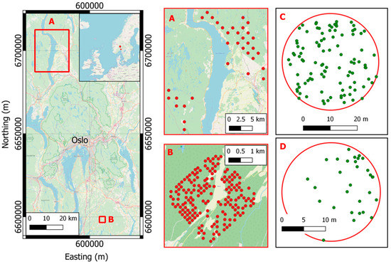
Figure 1.
Location of the two study areas: (A) Hadeland and (B) Våler. In panels A and B the field plots locations of Hadeland (A) and Våler (B) are shown. In panels C and D two examples of field plots with the tree positions in Hadeland (C) and Våler (D).

Table 1.
Statistics of the field data divided by species for the two datasets.
2.1. Hadeland Dataset
The field data were collected in 2016 on 13 circular sample plots of size 500 m2 and 21 circular sample plots of size 1000 m2 spread across a total area of about 1300 km2. Within each sample plot, tree species, DBH, and tree coordinates were recorded for all trees with DBH > 4 cm. All plots were positioned using static measurements and subsequent post-processing with data from a local base station. Two survey grade dual-frequency receivers, observing pseudo-range and carrier phase of both the Global Positioning System (GPS) and the Global Navigation Satellite System were used as rover and base units. The positions of the trees were measured in polar coordinates (distance and azimuth from the plot center). Height was measured for sample trees selected in each plot, and the heights of the non-sampled trees were predicted with a model constructed from the trees measured for height. A total of 3970 trees were recorded. AGB of each tree was calculated using the allometric models of Marklund [27].
Lidar data were acquired on 21st and 22nd of August 2015 using a Leica ALS70 laser scanner operated at a pulse repetition frequency of 270 kHz. The flying altitude was 1100 m above ground level. Up to four echoes per pulse were recorded, and the resulting density of single and first echoes was 5 m−2.
2.2. Våler Dataset
The field data were collected in 2010 on 152 circular sample plots of size 400 m2. Within each sample plot, tree species, DBH, and tree coordinates were recorded for all trees with DBH > 5 cm. All plots were positioned using static measurements and subsequent post-processing with data from a local base-station. Two survey grade dual-frequency receivers, observing pseudo-range and carrier phase of both the Global Positioning System (GPS) and the Global Navigation Satellite System were used as rover and base units. The positions of the trees were measured in polar coordinates (distance and azimuth from the plot center). A total of 9467 trees were recorded. The AGB of each tree was calculated using the allometric models of Marklund [27].
The lidar data were acquired on 9 September 2011 using a Leica ALS70 system operated with a pulse repetition frequency of 180 kHz. The flying altitude was of 1500 m above ground level. Up to four echoes per pulse were recorded, and the resulting density of single and first echoes was 2.4 m−2.
3. Methods
The proposed strategy is summarized in Figure 2, and it is based on the following steps:
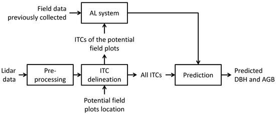
Figure 2.
Processing steps adopted in this study.
(1) define the possible field plots to survey according to a predefined sampling strategy (e.g., random and systematic);
(2) apply an ITC delineation method over the lidar data of the area of interest and assign the ITCs to the plots defined at step 1;
(3) on the basis of some pre-existing field data over the same area or a similar area, run the AL algorithm in order to define the best plot to survey and the best ITCs to survey inside the plot;
(4) go to the field and measure the trees (that corresponds to the ITCs delineated at step 2) suggested by the AL method;
(5) go back to step 3 and run again the AL method with the updated field data until the stopping criteria are reached.
In the following paragraphs, the processing steps are described with particular attention to the proposed AL for regression method (Section 3.3).
3.1. Lidar Data Preprocessing
A digital terrain model (DTM) was generated from the lidar echoes by the vendor using TerraScan software. The lidar point cloud was normalized to create a canopy height model (CHM) by subtracting the DTM from the z-values of the lidar echoes.
3.2. ITC Delineation
ITCs were delineated using an approach based on the lidar data and the delineation algorithm of the R package (itcSegment) [28,29]. The algorithm starts by first finding the local maxima within a rasterized CHM and designates them as treetops, and then uses a decision tree method to grow individual crowns around the local maxima. The final output of the algorithm is the detected ITCs with the height and crown area information. For more details about the algorithm, we refer the reader to [29].
The delineated ITCs were automatically matched to the trees in the field datasets. If only one field-measured tree was included inside an ITC, then that tree was associated with that ITC. In the case that more than one field-measured tree was included in a delineated ITC, the field-measured tree with the height most similar to the ITC height was chosen.
3.3. Proposed Active Learning System for Regression
3.3.1. Problem Definition
Let us assume that a training set D = is initially available, where N is the number of sample units, and each unit xi is represented by a vector in the d-dimensional measurement space and yi ∈ R is its corresponding target value. In our case, N corresponds to the number of ITCs available for the initial training set and the measurement space is their corresponding H and CD. The target value corresponds to the ground reference DBH (measured) and AGB (predicted). Given this training set D, we aim to predict an output value (DBH and/or AGB) of an unknown unit xi from a test set T = by using an interactive regression system as mentioned in Figure 3. This interactive method is based on selecting first at each iteration the best plot P’ and then select a batch B = of the best b sample units belonging to P’ from a larger set U = . of u unlabeled sample units, where b ≪ u. Those selected sample units are then associated with their output measures and added into the training set D. In Algorithm 1, a general description of the proposed method is presented. More details are provided in the following subsections.
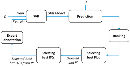
Figure 3.
Block diagram of the proposed interactive regression method.
| Algorithm 1: Interactive regression. |
| Input: Training set D = Unlabeled set U = Number of iterations: ITER Number of ITCs to label at each iteration b Output: predicted results of DBH and AGB Step 1: train the SVR using the training set D; for iter in 1: ITER Step 2: predict the output of the unlabeled sample units from U; Step 3: rank the ITCs and the plots based on diversity and cost criteria; Step 4: collect in the field the data for the top-ranked b ITCs from the selected plot; Step 5: increase the training set D with these new labeled sample units; Step 6: train the SVR using the updated dataset D; Step 7: output the final prediction results. |
3.3.2. Support Vector Regression
The proposed interactive method is based on the ε-insensitive support vector regression (SVR) method. SVR performs a linear regression in the feature space using an epsilon-insensitive loss (ε-SVR). This technique is based on the idea of deducing an estimate of the true, but unknown, relationship yi = g(xi) (i = 1, … , N) between the sample unit xi and its target value yi such that: (1) has, at most, ε deviation from the desired target yi; and (2) it is as smooth as possible. This is performed by mapping the data from the original feature space of dimension d to a higher d'-dimensional transformed feature space (kernel space), i.e., , to increase the flatness of the function and, by consequence, to approximate it in a linear way as follows:
Therefore, the SVR is formulated as the minimization of the following cost function:
subject to:
In the previous equations, it is supposed that the function is existing for each couple with a precision ε. However, in order to increase the generalization ability, some errors are acceptable. The concept of soft margin is introduced (see [30]) and the minimization problem will be formulated as minimization of the following cost function:
subject to:
where and are the slack variables that measure the deviation of the training sample unit outside the ε-insensitive zone. C is a parameter of regularization that allows tuning the tradeoff between the flatness of the function and the tolerance of deviations larger than ε.
The aforementioned optimization problem can be transformed through a Lagrange functional into a dual optimization problem expressed in the original dimensional feature space in order to lead to the following dual prediction model:
where K is a kernel function, S is a subset of indices (i = 1, …, N) corresponding to the nonzero Lagrange multipliers ’s or ’s. The training sample units that are associated to nonzero weights are called SVs. The kernel K(·,·) should be chosen such that it satisfies the condition imposed by the Mercer’s theorem, such as the Gaussian kernel functions [31,32]. In this study, the SVR implemented in the kernlab library [33] of the software R was used [34].
3.3.3. Ranking
During the training phase, we aim to find the best parameters by using the training set D so that the estimate has, at most, ε deviation from the desired targets . When the built model is applied to the unlabeled sample unit set U, the sample units that have a features distribution similar or close to that of the training sample units will give predicted output values close to their real ones, while the difference will be bigger for the sample units that have a very different feature distribution. Our objective is to select sample units from this last group and to add them to the training set in order to get more diversity among the training samples. This operation can help to create a more general model for regression and to get better results.
Let us suppose that is the constructed regression model using the training set D with the optimum parameters p, and let us suppose that is a similar model as with slightly changed parameters p’. By applying the trained model and the slightly modified model to the unlabeled set U = , we get:
Using the results obtained from (7) and (8), we can compute the diversity "v" as follows:
and also the inverse of the diversity "":
The diversity measure is used to rank the unlabeled sample units. The sample units with the highest diversity are more advantageous to be added to the training set D in order to improve the regression model .
3.3.4. Selecting Best Plot and Best ITCs
In field surveys, trees are usually measured in plots of a given size, and each plot can contain many trees and consequently many ITCs. For this reason, the selection strategy is based firstly on the selection of the best plot in each iteration, and then on the selection of the best b ITCs inside this plot. The main criteria used for the selection are the cost and the diversity . In our case, the cost is interpreted as the distance in meters that a person needs to travel in the forest in order to measure the selected trees. In order to find a tradeoff between the two measures ( and ), we opted for a Pareto-like optimization method which is inspired by the multi-objective optimization literature (MO optimization) and the non-dominated sorting concept [35,36,37].
3.3.5. Multi-Objective Optimization
In the presence of multiple measures of competing objectives that need to be simultaneously estimated, MO optimization can be solved by combining in a linear way the different objectives into a single function with fitting weights, or by finding a set of optimal solutions rather than just a single one. The selection of the best solution from this set is not trivial, and it is usually user-dependent. From a mathematical viewpoint, a general MO optimization problem can be formulated as follows: find the vector which minimizes the ensemble of objective functions:
subject to the I equality constraints:
and the J inequality constraints:
where p is a candidate solution to the considered optimization problem.
The MO optimization problem is solved using the concept of dominance. A solution is said to dominate another solution if and only if is partially smaller than , i.e.,
(1) for all indices
and
(2) for at least one index
This concept leads to the definition of Pareto optimality: a solution (Ω is the solution space) is said to be Pareto optimal if and only if there exists no other solution that dominates . The latter is said to be non-dominated and the set of all non-dominated solutions forms the so-called Pareto front of optimal solutions.
The final step, after the extraction of the Pareto front, is to select the final solution among the non-dominated ones. From the literature, we can find many strategies to extract this solution, and in the current study, we opted for the selection of the median solution in order to maintain a tradeoff between the two different criteria.
Figure 4 shows an example of a non-dominated sorting concept, in which a joint optimization of two criteria f1 (which represents in our case v′) and f2 (which represents the cost) is involved. The non-dominated samples (in red) constitute the Pareto front, which represents the set of optimal solutions (optimal samples). From this set, the selected solution is given by the median one (in green). Dominated solutions are drawn with black circles.
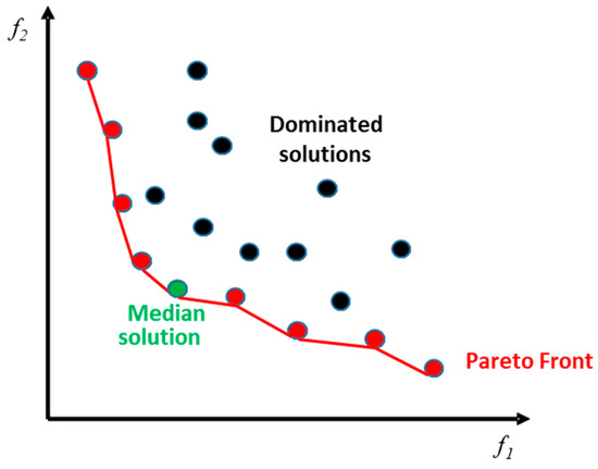
Figure 4.
Illustration of Pareto front solutions.
3.4. Performance Evaluation
In order to evaluate the proposed method, we adopted the root mean square error (RMSE):
where Nt is the total number of test sample units, and and are the field-reference and lidar-predicted output, respectively, for the ith test sample unit .
3.5. Design of the Experiments
In order to evaluate our method, each dataset (i.e., Hadeland, and Våler) was divided into two sets: training and test. The ITCs matched with the field measured trees of each species in each plot were sorted according to the DBH and one every second ITC was used for test and the rest for training. In this way, training and test sets had similar characteristics in terms of spatial distribution, species distribution, DBH, and AGB variation. For the Hadeland dataset, 607 sample units (ITCs) were used as training, and 627 sample units (ITCs) were used for testing, while for the Våler dataset, 1398 and 1245 ITCs were used for training and testing, respectively.
An outline of the different experiments accomplished in this study is presented in Table 2. In experiments A, B, and C, the training set of the Hadeland dataset was used as the initial training set D, while the training and the test sets of the Våler dataset were used as the unlabeled set U and the test set T, respectively. The total number of iterations was fixed to 20, and the maximum number of selected sample units in each iteration b was fixed to 10. The objective functions f1, related to the diversity, and f2, related to the cost, were computed in each iteration for each plot and the selected solution was the median of the Pareto front solutions. In order to have an additional evaluation of the proposed method, the position of the two datasets was permuted in experiments D, E, and F (see Table 2). In the latter case, due to the limited number of plots in the Hadeland dataset, the total number of iterations was fixed to 10 only, while the maximum number of selected sample units in each iteration b was fixed to 20. The criteria of samples selection were the same as the previous experiments.
Table 2.
Summary of the experiments carried out.
In experiments A, B, D and E, the prediction of DBH and AGB was done separately. From a practical point of view, such a way of prediction is costly especially when a person needs a double effort in order to measure trees existing inside a plot that is selected twice, first time for DBH prediction and the second time for AGB prediction. In order to reduce this cost, in experiments C and F, we predicted both DBH and AGB at the same time. In this case, two models were trained (one model for DBH and the other model for AGB) using the same training data. The final diversity, which will be considered for the next steps, was the average of diversities calculated for both models.
For comparison purposes, three other methods of selection were used: (1) Cost: minimization of the cost by selecting the closest plot from the current one at each iteration; (2) Diversity: selection of the plot that presents the maximum diversity in order to get the best accuracy; and (3) Rand: random selection.
Regarding SVR, the Radial Basis Function (RBF) was used as kernel functions. To compute the best parameter values, we use a cross-validation technique with a number of folds equal to three. During the cross-validation, the regularization parameter C of the SVR, and the width of its kernel function γ were varied in the range [1, 104] and [10−3, 5], respectively. The ε-value of the insensitive tube was fixed to 10−3.
4. Results
Table 3 shows the results obtained for the experiments A, B, and C using the four selection criteria. Regarding experiments A and B, we can see that the random selection criteria provided the worst results, with a very high cost and a small improvement in terms of RMSE compared to the initial case (the initial RMSE found by using the initial training D). Almost similar RMSEs were obtained by using only the Cost criterion for selection, with the advantage of having a very small cost. In contrast, when using only the Diversity criterion, the RMSEs improved but at a high cost. Using the MO Pareto optimization in order to find a compromise between the two criteria (Cost and Diversity), we can notice that the improvement in terms of RMSE is close to the one obtained by using only the Diversity criterion, but at a smaller cost (smaller distance).
Table 3.
Results obtained for Våler dataset (experiments A, B, and C). The initial RMSE is the RMSE obtained on Våler test set using only the Hadeland training set to build the model. The best results are highlighted in bold.
Regarding the results of experiment C (simultaneous prediction of both DBH and AGB), similarly to the previous results, the smallest RMSE was found by using the Diversity criterion but at a high cost. In contrast, using only the Cost criterion provided the minimum cost but with a large RMSE. A good compromise was found by using the MO Pareto optimization where the obtained RMSEs were close to those obtained by the Diversity criterion but at a smaller cost. The last remark concerning experiment C is that the obtained RMSEs were very close to those obtained in experiments A and B (predicting DBH and AGB separately) but at almost half of the cost.
In Figure 5 and Figure 6, the evolution of the RMSE and the cost during the different iterations is presented for the prediction of DBH and AGB using the different criteria. For both cases using the Diversity and the MO Pareto optimization, the graphs show a convergence toward better predictions with small fluctuations, contrary to the two other criteria (Rand and Cost criteria) where the variations are more marked. This phenomenon is due to the fact that in some iterations the selected sample units did not provide the expected improvement in the re-trained model, but they rather reduced the predictive ability of the model. Regarding the cost, we can notice from both figures that by using the MO Pareto and the Cost criteria for the selection we had a very low cost compared to the two other criteria (Rand and Diversity).
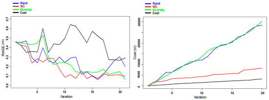
Figure 5.
Experiment A: Evolution of the RMSE (left panel) and the cost (right panel) for DBH prediction for the Våler dataset during the different iterations.
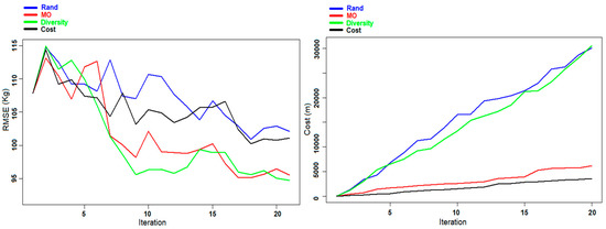
Figure 6.
Experiment B: Evolution of the RMSE (left panel) and the cost (right panel) for AGB prediction for the Våler dataset during the different iterations.
Figure 7 shows the evolution of the RMSE during the different iterations of experiment C. Similar to the previous experiments (A and B), the graphs of the Rand and Cost criteria show a large variation, which was due to the ineffective selection of samples in some iterations, and it was more stable and converged toward better predictions for the Diversity and MO Pareto criteria.
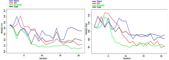
Figure 7.
Experiment C: Evolution of the RMSE of DBH (left panel) and AGB (right panel) for the Våler dataset during the different iterations.
As stated in the “Design of Experiments” Section, we also carried out three other experiments inverting the datasets that were used. The different results obtained for the prediction of DBH and AGB individually (experiments D and E) and together at the same time (experiment F) are presented in Table 4. The results are in line with the ones obtained in the previous three experiments (A, B, and C). From Table 4, we also conclude that using a method of optimization to reach a compromise between accuracy and cost is the best way in order to get good results at the minimum cost possible. Figure 8 and Figure 9 present the evolution of the RMSE and the cost as a function of the number of iterations for the experiments D and E, respectively. In the case of the DBH prediction, the MO Pareto criterion is always providing the lowest RMSE at each iteration, and almost always the lowest cost: the lowest cost is obviously provided by the Cost criterion. The Rand approach is providing the worst results for both RMSE and cost. In the case of AGB (Figure 9) the RMSE of the Diversity criterion is providing slightly better results with respect to the MO Pareto criterion. Figure 10 shows the results obtained for the experiment F. As in experiment C there is a higher variation at each iteration, with some cases where some selected samples are decreasing the performance of the predictor.
Table 4.
Results obtained for the Hadeland dataset (experiments D, E, and F). The initial RMSE is the RMSE obtained on Hadeland test set using only the Våler training set to build the model. The best results are highlighted in bold.
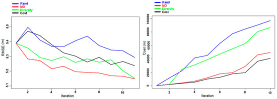
Figure 8.
Experiment D: Evolution of the RMSE (left panel) and the cost (right panel) of DBH prediction for the Hadeland dataset during the different iterations.
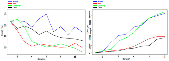
Figure 9.
Experiment E: Evolution of the RMSE (left panel) and the cost (right panel) of AGB prediction for the Hadeland dataset during the different iterations.
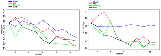
Figure 10.
Experiment F: Evolution of the RMSE of DBH (left panel) and AGB (right panel) for the Hadeland dataset during the different iterations.
5. Discussion
In this paper, we proposed a new method based on AL for improving field data collection for the prediction of DBH and AGB at ITC level. The proposed method was shown to be effective as it allowed to improve the prediction accuracy compared to pure random sampling while also reducing the cost in terms of distance traveled in the forest. The proposed approach has margins for improvement as the current cost function is based only on distance while in a real context it should consider the roads and paths network of the study area and if the distance can be traveled on foot or by car (like in Demir et al. [38]), but it still represents a good example of how field data collection could be improved introducing advanced machine learning methods, like AL. Compared to a conventional field data survey the proposed approach requires a total change in how it is planned. The selection of sample units should be made after the lidar data have been collected, and it is required to have the possibility to retrain the model after each selection of new sample units. In particular, it is necessary that the field crew have access to a processing system through a tablet or a smartphone in order to run the AL system. Another point to consider is the localization of the trees suggested by the AL system. In this case, the knowledge, additionally to the position, of the height and DBH predicted by the AL system could speed up the localization procedure. As the AL system will suggest measuring only trees visible from above the forest, in case of a not very dense forest, or a mature forest, and in particular in boreal and temperate forests, the localization procedure could be done just using a priori information like the CHM of the area and the terrain contour lines, without the use of a highly accurate GPS device.
The topic of the use of remote sensing data to optimize the field data collection design have been widely studied [39,40,41]. Normally remote sensing data are used to stratify the distribution of the samples, and to help in the selection of the most suitable samples, and once they are defined the field data collection is carried out without any updating phase. The main difference among these methods and the AL methods is that in the AL systems the model optimization is also involved in the choice and also the data collection cost.
All the four methods considered allow to improve the prediction accuracy compared to the use of only the initial training set. This was expected as obviously adding samples of the area under analysis is improving the prediction accuracy, compared to use only sample units from a similar area located in another place. Another expected result is that the Rand approach is always giving the worst results in terms of both cost and accuracy, while the one based on Diversity is always providing the best results in terms of accuracy. The MO Pareto optimization is the one having the best trade-off between the RMSE and the cost, and this method is the one having more potential in the context of forest inventories. Moreover, according to the needs, other parameters could be added to the optimization considering thus not only the RMSE and the distance. Despite this, the choice of the selection strategy should be made according to the final user needs: if the budget is limited a selection based on the Cost is essential, while if the objective is to have the best possible prediction accuracy, independently from the cost, the choice should be based on the Diversity.
In this study, the potential plots to be selected by the AL method were systematically distributed over the two study areas as they were used for previous studies, and forest inventory purposes. We used thus a possible grid of plots to visit, defined according to sampling design, and then only certain plots, and certain trees inside the plots were sampled. The proposed AL system could also work with a totally random sampling design. This is the usual approach used in AL methods based on photointerpretation [16]. In the specific case analyzed in this study, a random approach with many possible candidate plots could be actually more effective for the AL system as it allows for much more potential plots to choose from. The drawback could be that the plots selected will not respect any sampling design, and they could not cover the entire spatial distribution of the study area. Moreover, the proposed AL method could also work independently from the plots by selecting the best ITCs directly over the entire area. In this case, the suggested approach should be to delineate ITCs over the entire area and then either to use the position of each ITC as a possible candidate sample unit, or to sample the ITCs according to sampling design, and then survey only the ones suggested by the AL system.
As we showed in this study, changing the target variable could lead to the selection of different sample units and to have a different final training set, that would not necessarily be suitable for the prediction of other variables. In practical, such an issue should be kept in mind in order to survey plots and ITCs that are useful for all the needed predictions. In the case where the variables to predict are correlated, like DBH and AGB, the candidate sample units will be in any case similar, while in the case where the variables to predict are not correlated there may be in any case the possibility to carry on disjoint AL-based field surveys.
6. Conclusions
In this study, a new method of active learning for regression based on selecting the best field sample units was presented. The method of regression used is the support vector regression, and the criteria of selection are based on the accuracy and the cost. The accuracy criteria use the diversity of the unlabeled sample units while the cost is considered as the distance traveled by the expert to label the selected units. The developed method was applied to predict the DBH and the AGB using the height of the trees and their crown diameter as independent variables. Those two last variables are directly extracted from lidar data while DBH and AGB need to be measured/predicted in the field. The experimental results show the effectiveness of the proposed selection strategy to give better results with substantial improvements over the different iterations. We observed that the proposed method converged to a low RMSE with a considerably lower cost compared to using a random selection method.
The proposed method can be applied to any learning problem where the cost of labeling selected sample units is an important factor to be taken into consideration. This is the case when labeling queried sample units depends on the previously annotated ones.
Author Contributions
Conceptualization, S.M. and M.D.; methodology, S.M..; resources, F.M. and D.G.; data curation, T.G. and E.N.; writing—original draft preparation, S.M. and M.D.; writing—review and editing, S.M., M.D., T.G., E.N., F.M. and D.G.; supervision, M.D.; project administration, F.M. and D.G.; funding acquisition, M.D., T.G., and E.N.
Funding
This work was funded by the HyperBio project (project 244599) funded by the BIONÆR program of the Research Council of Norway and by TerraTec AS, Norway.
Conflicts of Interest
The authors declare no conflict of interest.
References
- Englin, J.; Callaway, J.M. Global climate change and optimal forest management. Nat. Resour. Model. 1993, 7, 191–202. [Google Scholar] [CrossRef]
- Melillo, J.M.; McGuire, A.D.; Kicklighter, D.W.; Moore, B.; Vorosmarty, C.J.; Schloss, A.L. Global climate change and terrestrial net primary production. Nature 1993, 363, 234–240. [Google Scholar] [CrossRef]
- IPCC Guidelines for National Greenhouse Gas Inventories. Agric. For. Other L. Use. 2006. Available online: https://www.ipcc-nggip.iges.or.jp/meeting/pdfiles/Washington_Report.pdf (accessed on 1 March 2019).
- Hyink, D.M.; Moser, J.W., Jr. Generalized Framework for Projecting Forest Yield and Stand Structure Using Diameter Distributions. For. Sci. 1983, 29, 85–95. [Google Scholar]
- White, J.C.; Coops, N.C.; Wulder, M.A.; Vastaranta, M.; Hilker, T.; Tompalski, P. Remote Sensing Technologies for Enhancing Forest Inventories: A Review. Can. J. Remote Sens. 2016, 42, 619–641. [Google Scholar] [CrossRef]
- Maltamo, M.; Næsset, E.; Vauhkonen, J. (Eds.) Forestry Applications of Airborne Laser Scanning; Springer: Dordrecht, The Netherlands, 2014; Volume 27. [Google Scholar]
- Næsset, E. Estimating timber volume of forest stands using airborne laser scanner data. Remote Sens. Environ. 1997, 61, 246–253. [Google Scholar] [CrossRef]
- Næsset, E. Predicting forest stand characteristics with airborne scanning laser using a practical two-stage procedure and field data. Remote Sens. Environ. 2002, 80, 88–89. [Google Scholar] [CrossRef]
- Hyyppä, J.; Kelle, O.; Lehikoinen, M.; Inkinen, M. A segmentation-based method to retrieve stem volume estimates from 3-D tree height models produced by laser scanners. IEEE Trans. Geosci. Remote Sens. 2001, 39, 969–975. [Google Scholar] [CrossRef]
- Maltamo, M.; Mustonen, K.; Hyyppä, J.; Pitkänen, J.; Yu, X. The accuracy of estimating individual tree variables with airborne laser scanning in a boreal nature reserve. Can. J. For. Res. 2004, 34, 1791–1801. [Google Scholar] [CrossRef]
- MacKay, D.J.C. Information-Based Objective Functions for Active Data Selection. Neural Comput. 1992, 4, 590–604. [Google Scholar] [CrossRef] [Green Version]
- Cohn, D.; Atlas, L.; Ladner, R. Improving generalization with active learning. Mach. Learn. 1994, 15, 201–221. [Google Scholar] [CrossRef] [Green Version]
- Cohn, D.A.; Ghahramani, Z.; Jordan, M.I. Active Learning with Statistical Models. J. Artif. Intell. Res. 1996, 4, 129–145. [Google Scholar] [CrossRef]
- Pasolli, E.; Melgani, F. Active learning methods for electrocardiographic signal classification. IEEE Trans. Inf. Technol. Biomed. 2010, 14, 1405–1416. [Google Scholar] [CrossRef]
- Rahhal, M.M.A.; Bazi, Y.; Alhichri, H.; Alajlan, N.; Melgani, F.; Yager, R.R. Deep learning approach for active classification of electrocardiogram signals. Inf. Sci. 2016, 345, 340–354. [Google Scholar] [CrossRef]
- Tuia, D.; Ratle, F.; Pacifici, F.; Kanevski, M.F.; Emery, W.J. Active learning methods for remote sensing image classification. IEEE Trans. Geosci. Remote Sens. 2009, 47, 2218–2232. [Google Scholar] [CrossRef]
- Demir, B.; Persello, C.; Bruzzone, L. Batch-mode active-learning methods for the interactive classification of remote sensing images. IEEE Trans. Geosci. Remote Sens. 2011, 49, 1014–1031. [Google Scholar] [CrossRef]
- Syed, A.R.; Rosenberg, A.; Kislal, E. Supervised and unsupervised active learning for automatic speech recognition of low-resource languages. In Proceedings of the ICASSP, IEEE International Conference on Acoustics, Speech and Signal Processing, Shanghai, China, 20–25 March 2016. [Google Scholar]
- Yu, D.; Varadarajan, B.; Deng, L.; Acero, A. Active learning and semi-supervised learning for speech recognition: A unified framework using the global entropy reduction maximization criterion. Comput. Speech Lang. 2010, 24, 433–444. [Google Scholar] [CrossRef]
- Sun, Z.; Ye, Y.; Zhang, X.; Huang, Z.; Chen, S.; Liu, Z. Batch-mode active learning with semi-supervised cluster tree for text classification. In Proceedings of the 2012 IEEE/WIC/ACM International Conference on Web Intelligence, Macau, China, 4–7 December 2012. [Google Scholar]
- Zhu, W.; Allen, R.B. Active learning for text classification: Using the LSI subspace signature model. In Proceedings of the DSAA 2014 IEEE International Conference on Data Science and Advanced Analytics, Shanghai, China, 30 October–1 November 2014. [Google Scholar]
- Chang, Y.H.; Thibault, G.; Madin, O.; Azimi, V.; Meyers, C.; Johnson, B.; Link, J.; Margolin, A.; Gray, J.W. Deep learning based Nucleus Classification in pancreas histological images. In Proceedings of the Annual International Conference of the IEEE Engineering in Medicine and Biology Society, EMBS, Seogwipo, Korea, 11–15 July 2017. [Google Scholar]
- Shao, W.; Sun, L.; Zhang, D. Deep active learning for nucleus classification in pathology images. In Proceedings of the International Symposium on Biomedical Imaging, Washington, DC, USA, 4–7 April 2018. [Google Scholar]
- Cai, W.; Zhang, Y.; Zhou, J. Maximizing expected model change for active learning in regression. In Proceedings of the IEEE International Conference on Data Mining, ICDM, Dallas, TX, USA, 7–10 December 2013. [Google Scholar]
- Demir, B.; Bruzzone, L. A multiple criteria active learning method for support vector regression. Pattern Recognit. 2014, 47, 2558–2567. [Google Scholar] [CrossRef]
- Persello, C.; Boularias, A.; Dalponte, M.; Gobakken, T.; Naesset, E.; Scholkopf, B. Cost-sensitive active learning with lookahead: Optimizing field surveys for remote sensing data classification. IEEE Trans. Geosci. Remote Sens. 2014, 52, 6652–6664. [Google Scholar] [CrossRef]
- Marklund, L.G. Biomass Functions for Pine, Spruce and Birch in Sweden; Rapp. Sveriges Lantbruksuniversitet, Institutionen foer Skogstaxering. 1988. Available online: http://agris.fao.org/agris-search/search.do?recordID=SE8811514 (accessed on 1 March 2019).
- Dalponte, M. Package itcSegment. 2018. Available online: https://cran.r-project.org/web/packages/itcSegment/itcSegment.pdf (accessed on 18 April 2019).
- Dalponte, M.; Coomes, D.A. Tree-centric mapping of forest carbon density from airborne laser scanning and hyperspectral data. Methods Ecol. Evol. 2016, 7, 1236–1245. [Google Scholar] [CrossRef] [PubMed]
- Cortes, C.; Vapnik, V. Support-Vector Networks. Mach. Learn. 1995, 20, 273–297. [Google Scholar] [CrossRef]
- Vapnik, V.N. An overview of statistical learning theory. IEEE Trans. Neural Networks 1999, 10, 988–999. [Google Scholar] [CrossRef]
- Smola, A.J.; Schölkopf, B. A tutorial on support vector regression. Stat. Comput. 2004, 14, 199–222. [Google Scholar] [CrossRef] [Green Version]
- Karatzoglou, A.; Smola, A.; Hornik, K.; Zeileis, A. Kernlab—An S4 Package for Kernel Methods in R. J. Stat. Softw. 2015, 11, 1–20. [Google Scholar] [CrossRef]
- R Core Team. R: A Language and Environment for Statistical Computing; R Foundation for Statistical Computing: Vienna, Austria, 2017. [Google Scholar]
- Laundy, R.S.; Steuer, R.E. Multiple Criteria Optimisation: Theory, Computation and Application. J. Oper. Res. Soc. 1988, 39, 879. [Google Scholar] [CrossRef]
- Stadler, W. A survey of multicriteria optimization or the vector maximum problem, part I: 1776–1960. J. Optim. Theory Appl. 1979, 29, 1–52. [Google Scholar] [CrossRef]
- Mardle, S.; Miettinen, K.M. Nonlinear Multiobjective Optimization. J. Oper. Res. Soc. 2006, 51, 246. [Google Scholar] [CrossRef]
- Demir, B.; Minello, L.; Bruzzone, L. Definition of effective training sets for supervised classification of remote sensing images by a novel cost-sensitive active learning method. IEEE Trans. Geosci. Remote Sens. 2014, 52, 1272–1284. [Google Scholar] [CrossRef]
- Hawbaker, T.J.; Keuler, N.S.; Lesak, A.A.; Gobakken, T.; Contrucci, K.; Radeloff, V.C. Improved estimates of forest vegetation structure and biomass with a LiDAR-optimized sampling design. J. Geophys. Res. Biogeosci. 2009, 114, 1–11. [Google Scholar] [CrossRef]
- Maltamo, M.; Bollandsås, O.M.; Næsset, E.; Gobakken, T.; Packalén, P. Different plot selection strategies for field training data in ALS-assisted forest inventory. Forestry 2011, 84, 23–31. [Google Scholar] [CrossRef]
- Dalponte, M.; Ene, L.T.; Ørka, H.O.; Gobakken, T.; Naesset, E. Unsupervised selection of training plots and trees for tree species classification. In Proceedings of the International Geoscience and Remote Sensing Symposium (IGARSS), Melbourne, Australia, 21–26 July 2013. [Google Scholar]
© 2019 by the authors. Licensee MDPI, Basel, Switzerland. This article is an open access article distributed under the terms and conditions of the Creative Commons Attribution (CC BY) license (http://creativecommons.org/licenses/by/4.0/).