Article

Effects of UAV Image Resolution, Camera Type, and Image Overlap on Accuracy of Biomass Predictions in a Tropical Woodland

1
GEOFOREST-IUCA, Department of Geography, University of Zaragoza, Pedro Cerbuna 12, 50009 Zaragoza, Spain
2
Faculty of Environmental Sciences and Natural Resource Management, Norwegian University of Life Sciences, P.O. Box 5003, NO-1432 Ås, Norway
3
Department of Forestry, Lilongwe University of Agriculture and Natural Resources, P.O. Box 219, Lilongwe, Malawi
*
Author to whom correspondence should be addressed.
Remote Sens. 2019, 11(8), 948; https://doi.org/10.3390/rs11080948
Submission received: 21 February 2019 / Revised: 13 April 2019 / Accepted: 17 April 2019 / Published: 19 April 2019
(This article belongs to the Special Issue UAV Applications in Forestry)

Abstract

:
Unmanned aerial systems (UASs) and photogrammetric structure from motion (SFM) algorithms can assist in biomass assessments in tropical countries and can be a useful tool in local greenhouse gas accounting. This study assessed the influence of image resolution, camera type and side overlap on prediction accuracy of biomass models constructed from ground-based data and UAS data in miombo woodlands in Malawi. We compared prediction accuracy of models reflecting two different image resolutions (10 and 15 cm ground sampling distance) and two camera types (NIR and RGB). The effect of two different side overlap levels (70 and 80%) was also assessed using data from the RGB camera. Multiple linear regression models that related the biomass on 37 field plots to several independent 3-dimensional variables derived from five UAS acquisitions were constructed. Prediction accuracy quantified by leave-one-out cross validation increased when using finer image resolution and RGB camera, while coarser resolution and NIR data decreased model prediction accuracy, although no significant differences were observed in absolute prediction error around the mean between models. The results showed that a reduction of side overlap from 80 to 70%, while keeping a fixed forward overlap of 90%, might be an option for reducing flight time and cost of acquisitions. Furthermore, the analysis of terrain slope effect in biomass predictions showed that error increases with steeper slopes, especially on slopes greater than 35%, but the effects were small in magnitude.

Graphical Abstract

1. Introduction

Tropical forests play a major role in world carbon storage [1], while providing biodiversity and ecological services [2]. Efforts to implement mechanisms that reduce forest deforestation and degradation such as REDD+ could help to stabilize CO2 atmospheric concentrations [1]. The REDD+ mechanism is in the preliminary phases in 33 tropical countries requiring the establishment of administrative structures and the determination of reference levels for carbon stocks [3]. Malawi, as an example, is targeting 112 small- to medium-sized forest reserves with sizes of up to 2240 ha scattered across the country as potential REDD+ project areas [3]. Carbon stock estimation in these forest reserves requires design and implementation of statistically sound and consistent forest inventories [4]. Field-based forest inventories, which often are associated with large operational and logistical costs, can benefit from remotely sensed information to reduce costs while improving precision of the estimates [5,6,7].
Remote sensing technologies been effective in estimating forest resource parameters such as biomass [8,9]. Particularly, airborne laser scanning (ALS) has shown great potential for forest biomass estimation in different forest types, including boreal [10], temperate [11], Mediterranean [12] and tropical forests [13]. Recently, the use of unmanned aircraft systems (UASs) and the improvement of structure from motion (SfM) algorithms [14] have provided opportunities for new cost-effective alternatives to estimate forest attributes for smaller geographical areas [15,16]. SfM is a computer vision technique developed from traditional photogrammetric techniques [2] that derive 3D point clouds from very-high resolution images including ground-based images. SfM algorithms generate 3D geometry from many viewpoints of overlapping images without the need to have calibrated cameras [17]. UAS point clouds, characterized by a high point density, are mostly associated with the exterior of the canopy. Nevertheless, UAS data have been useful for estimation of forestry variables either by using a digital terrain model (DTM) derived from ALS [17,18,19,20] or a DTM derived from the UAS images to normalize the point cloud [3,18,21,22,23], or by simply using raw non-normalized photogrammetric data [24]. Previous studies have demonstrated estimation of individual tree variables such as tree height [15,25,26], canopy cover [15], crown diameter [15], tree density [15,25], diameter [25], biomass [25], canopy fuels [16], or tree detection [27,28,29]. Furthermore, UAV have been used for the estimation of height [17,21], number of stems [17], basal area [17], volume [17,29,30], canopy cover [31,32] and biomass [3,21,22], canopy gap detection [31,33,34], or tree-stump detection [35] using an area-based approach.
Field data collection and modeling of forest attributes, including variable selection, parametrization and processing, are a significant part of the total cost in UAV-based inventories. Model transferability was proposed to extrapolate models fitted for one area to other area (spatial transferability) [36] or to other points in time (temporal transferability) [37] for reducing the costs. For example, multi-temporal ALS data have been used to temporally transfer a model between two points in time using the direct approach (e.g., [11,38,39,40,41,42]). A similar approach might be considered to transfer a model fitted for a UAS acquisition, with a specific flight configuration, to other acquisitions with different flight configurations (e.g., different image resolution, camera type, side overlap) to reduce modeling costs.
Research on the effects of technical properties of the flight configuration, use of different camera systems, data processing options and the amount and properties of the field data used to establish relationships between ground data and UAS-derived point cloud data is limited. However, these are important considerations when designing UAS surveys to support forest inventories, because they may affect both costs and the accuracy of the results. Dandois et al. [43] did, however, analyze the effects of altitude, overlap and weather conditions on estimation of height and biomass by using an RGB (red-green-blue) camera. Fraser et al. [44] and Torres-Sánchez [45] found that a 100 m flight altitude was superior when compared to up to 120 m above ground. An analysis of forward overlap effects as associated with resolution or flight altitude was performed by Dandois et al. [43], Frey et al. [44] and Torres-Sánchez [45] whose showed that larger levels of forward overlap increased accuracy. Ni et al. [46] also found that finer image resolutions required larger forward overlaps. Furthermore, Dandois et al. [43] and Fraser et al. [44] compared different processing algorithms, but small differences were revealed. Kachamba et al. [22] compared the use of different filters to generate a digital terrain model (DTM) from UAS images. The influence of slope in DTM precision and accuracy of forestry attributes [47,48] have been analyzed using ALS sensors. Although ALS model predictions were affected by the increase in slope when estimating tree height [48,49,50], tree top detection [51], tree diameter, basal area, number of stems and volume [48], the effects were not severe. The successful estimation of forest attributes using 3D photogrammetric point clouds, which yield high point densities located mostly in the top of the canopy, might also be affected by slope. The analysis of plot size effects on the precision of biomass estimates in a dry tropical forest carried out by Kachamba et al. [3] determined that larger sample plot sizes of 1000 m2 tend to favor UAS-assisted inventories. The effects of several other important factors, as listed in Dandois et al. [23], remains unknown. Among these are camera type and image resolution acquired by UASs acquisition. To the best of our knowledge, the effects of these variables for estimating forest attributes remain unexplored. We examined two camera types in this manuscript that capture data in different regions of the electromagnetic spectrum, specifically only including the visible range of the spectrum: blue, green, and red (RGB) bands or including the near infrared (NIR) spectrum: green, red, and near-infrared bands.
The main goal of this study was to analyze the effects of camera type, image resolution, side overlap, and some practical considerations that often have to be made in operational surveys on accuracy of biomass model predictions in a tropical woodland using an UAS. Specifically, we aimed to quantify the effects of: (1) two different RGB and NIR cameras capturing two image resolutions of 10 and 15 cm ground sample distance (GSD), respectively, (2) two levels of side overlap: 70% and 80% using the RGB camera only, (3) transferability of models fitted from one set of acquisition parameters to other acquisitions, which were acquired with different flight characteristics and/or camera types, and (4) terrain slope on biomass predictions.

2. Materials and Methods
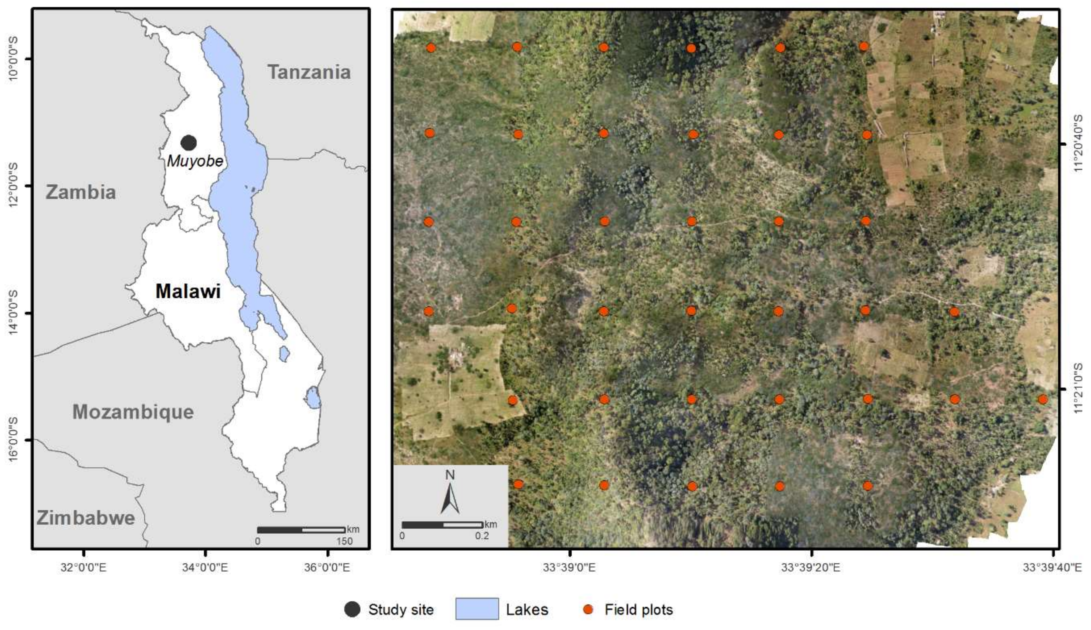
2.1. Study Area

The miombo woodlands in this study are part of the Muyobe community forest reserve, located in Mpherembe traditional authority in Mzimba district in the northern region of Malawi (centered at 11°35′S, 33°65′E, 1169–1413 m above sea level) (Figure 1). The selected area constitutes 200 ha of a total of 486 ha of the reserve. The dominant soil type is Ferrosols [48]. The mean annual daily minimum and maximum temperatures are 15 ± 1.6 °C and 26 ± 0.6 °C, respectively, and the annual rainfall was 889 ± 146 mm for the period 1975–2005. The dominant tree species in terms of biomass are Mnondo (Julbernadia globiflora), Mukongolo (Brachystegia manga) and Muwombo (Brachystegia longifolia), accounting for 20%, 12%, and 10% of the total biomass, respectively. For more details on the study area, see Kachamba et al. [32].

2.2. Field Measurements

Field data were acquired in 37 circular plots with 17.84 m radius (0.1 ha each) during April to May of 2015. A systematic sampling design was adopted with grids of 220 m by 220 m. The center of each of the designated plots was precisely located in the field using differential Global Navigation Satellite System (dGNSS). Two Topcon legacy-E + 40 channels dual frequency receivers were used with pseudo-range and carrier phase of global positioning system (GPS) and Global Navigation Satellite System (GLONASS). One receiver was used as a base station, while the other was used as a rover field unit within a baseline of 25 km. As proposed by Kouba [52], the base station position was established using precise point positioning with GPS and GLONASS data collected continuously for 24 h. The rover field unit was placed at the center of each plot on a rod at 2.98 m above ground level and data were recorded for an average of 33 ± 20 min using a one-second logging rate. The RTKLIB open source software version 2.4.2 developed by Takasu [53] was used for post-processing the recorded sample plot center coordinates. The maximum standard deviation revealed for northing, easting and height coordinates were 0.22 cm, 0.56 cm and 0.42 cm, respectively.
The diameter at breast height (dbh) was measured using a caliper or a diameter tape. A Haglöf Sweden® Vertex instrument was used for measuring total tree heights of up to 10 randomly selected sample trees within each plot. A height-diameter model developed by Kachamba and Eid [54] for the inventoried species in 107 sample plots systematically distributed along the entire Muyobe community forest reserve was used in this study. Among the 107 samples, we used 37 sample plots in this study for predicting tree height for those trees for which tree height was not measured. Then, aboveground biomass was predicted for the individual trees in each sample plot using the biomass allometric model developed by Kachamba et al. [22] for the 33 most representative species for miombo woodlands in Malawi, including these present in the study area, with diameter at breast height and tree height as independent variables. Subsequently, the tree biomass values were summed to obtain plot-level biomass values that were subsequently scaled to per-hectare values and used as ground reference value. Table 1 shows statistical summary of the field plot characteristics.

2.3. Remotely Sensed Data Collection and Processing

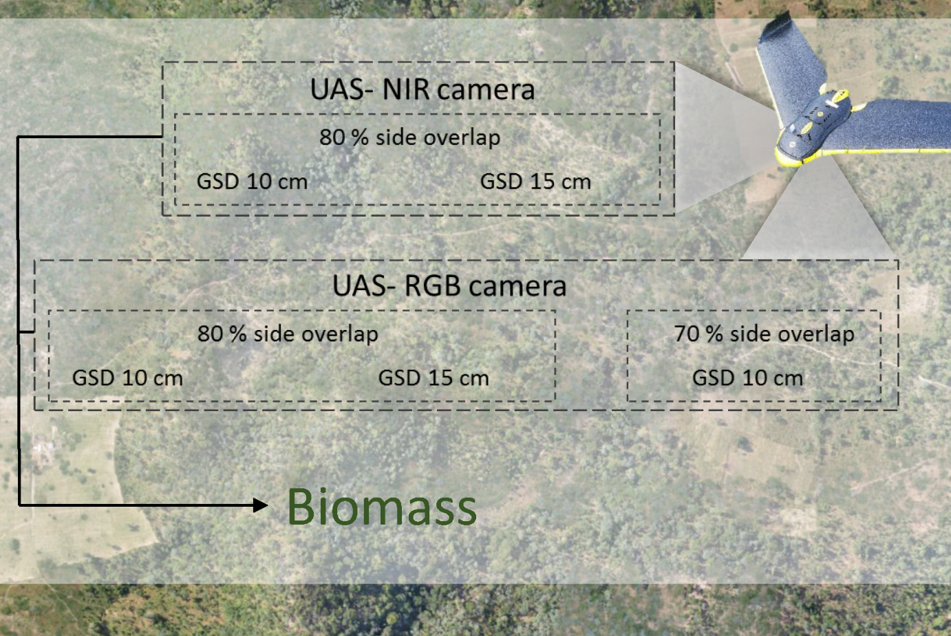
2.3.1. UAS Imagery Collection

The UAS images were collected from 23 to 26 April 2015, a leaf-on immediately following the rainy season. The images were collected using a SenseFly eBee fixed-wing UAS [55] equipped with two different types of cameras, which were used separately (Table 2). The RGB camera was a Canon IXUS127 HS (Canon Inc., Tokyo, Japan) with a dimension of 93.2 × 57.0 × 20.0 mm and a weight of 135 g with memory card and battery included. The sensor produces three separate 16.1 megapixel images in the red (660 nm), green (520 nm) and blue (450 nm) bands. The NIR (near infra-red) camera was a Canon S110 (Canon Inc., Tokyo, Japan) with a size of 74.4 × 55.8 mm and a weight of 153 g, including memory card but not the battery. The sensor produces three separate 12.1 megapixel images in the green (550 nm), red (625 nm) and NIR (850 nm) spectral bands. The eBee platform has a weight of 537 g without payload and it was equipped with an inertial measurement unit (IMU) and a GNSS to control the flight parameters and provide positioning during flight operations [55].
Prior to the image acquisition, the positions of 11 ground control points (GCPs) were determined and measured using the same procedure as the one used to establish the location of the sample plot centers for the field inventory. The GCP targets consisted of a set of 1 × 1 m cross-shaped timber planks painted white and some with black and white 50 × 50 cm checkerboard markers. GNSS position data for each GCP target were recorded for an average of 13 ± 6 min for each GCP with a one-second logging rate and post-processed using the RTKLIB software. The average standard deviation reported for northing, easting and height coordinates were 0.56 cm, 1.28 cm and 1.12 cm, respectively.
The image acquisition was controlled using the eMotion 2 version 2.4 software (Sensefly, Ltd., Cheseaux-Lausanne, Switzerland) [55] installed on a laptop computer. The flights were planned prior to flight using the mission control software and georeferenced base map from Microsoft Bing. Flight altitude above ground was determined according to the camera spectral sensitivity to generate constant 10 and 15 cm GSD pixel resolution images (Table 2). The acquisition of 10 cm GSD pixel images using the IXUS127 HS camera was carried out at 325 m above ground, but 286 m above ground when using the Canon S110 camera. Similarly, the acquisition of 15 cm GSD pixel images with the IXUS127 HS camera was carried out at 487 m above ground, but 430 m above ground when using the Canon S110 camera. This solution was adopted as cameras with similar sensitivities was not available for the present analysis. The five acquisitions were performed by keeping a fixed forward overlap of 90%, which refers to the overlap between consecutive images within a flight strip. The details of each acquisition are shown in Table 2. Side overlap, which refers to the overlap between images in adjacent flight strips, was set to 80% for the NIR-10, NIR-15, RGB-10 and RGB-15 acquisitions (Table 2). However, a side overlap of 70% was chosen for RGB-10-L. In total, 18 flights were carried out. These side overlap values were chosen taking into account stereo-matching requirements, previous flight experiences and considering additional flight time restrictions. Nine flights was performed for RGB-10 acquisition resulting in the larger number of images (1691) and the increase of flight time compared to other acquisitions. These flights were taken during days 23, 24 and 25 of April 2015, being part of previous analysis carried out by Kachamba et al. [3,22] for the entire Muyobe community forest reserve. The flight planning area was different for this acquisition, including images from nine flights to capture all the analyzed area for the present study.

2.3.2. Image Processing

The generation of three-dimensional (3D) dense point clouds from the images were performed for each acquisition using the proprietary software Agisoft Photoscan Professional version 1.1 (Agisoft LLC., St. Petersburg, Russia) [56]. Acquisitions were processed individually assigning the master band Red to the Canon IXUS127 HS camera and NIR to the Canon S110 camera. This software includes structure from motion (SfM) and stereo-matching algorithms to align the images and perform multi-view stereo reconstruction. The creation of the 3D point clouds required the following processing steps: (i) image alignment using the SfM techniques to reconstruct the 3D geometry by detecting and matching image feature points in overlapping images [17]; (ii) guided marker positioning and camera optimization alignment: GCP coordinates were imported and the estimated positions, provided by the GNSS onboard the SenseFly eBee, were refined manually, which improved the position, as well as the camera orientation. The final positioning accuracy was 0.23, 0.19, 0.21, 0.23 and 0.22 m for the NIR-10, NIR-15, RGB-10, RGB-15 and RGB-10-L, respectively; and (iii) building the dense point clouds. The parameters used for the processing steps i-iii are shown in Table 3 and they were based on the empirical analysis by Puliti et al. [17]. Spectral information from the imagery (red, green and blue bands for the RGB camera and red, green and near-infrared for the NIR camera) was added to the point cloud. Spectral information from UAS point clouds has, in previous studies, been found useful for estimating non-structural properties of the canopy [18], as well as properties such as biomass [3,22].

2.3.3. DTM Generation

Point cloud classification was performed using a two-phase approach: (a) application of the progressive triangulated irregular network (TIN) algorithm developed by Axelsson [57]; and (b) application of the KDTree filter developed by Maneewongvatana and Mount [58] to reclassify ground points keeping only the lowest in a circular area approximately of the size of the crowns. First, the variant of the progressive TIN implemented in Agisoft Photoscan software [52] was applied. The algorithm divides the point cloud into cells of a certain size detecting the lowest point and generating a first approximate terrain model by triangulation. A cell size of 50 m was applied in the study. Then, the angle and maximum distance between a point and the DTM surface was set. In this study, a grid search approach was applied to test different values for angle parameters, considering a fixed maximum distance of 1 m. Based on preliminary tests, a 20-degree angle was chosen for further testing, and a ground-filtered point cloud was generated using that angle for the different acquisitions. Second, the KDTree filter was applied. This filter is included in the scipi.spatial library, and it was implemented in Python. KDTree is a binary tree whose nodes represent an axis-aligned hyper-rectangle. The set of points are split by each node by specifying an axis following the “sliding midpoint” rule [59]. A maximum distance of 5 m was set for accounting only for the closest neighbors considering crown size. The resulting DTM was then used to calculate the height relative to the ground for all points by subtracting the respective TIN values from the elevation of each point. The use of two subsequent filters determined spurious points below the average ground elevation, which are commonly associated with point clouds derived using SfM [60], being removed from further analysis and variable computation.

2.3.4. Variable Computation

A total of 86 point cloud variables commonly used as independent variables in forestry studies, were computed for each field plot and acquisition [12,22]. They characterized canopy height, canopy density, and canopy spectral properties. Variables describing canopy height and canopy density were extracted as described by Næsset [61] and McGaughey [62]. Canopy height variables include minimum (Hmin), maximum (Hmax), mean (Hmean), mode (Hmode), standard deviation (Hsd), coefficient of variation (Hcv), kurtosis (Hkurt), skewness (Hskewness), variance (Hvariance) and height percentiles (H01, H10, H20, H25, H30, H40, …, H70, H75, H80, H90, H95, H99). In accordance with Kachamba et al. [3,22], a threshold value of 0.5 m height was applied to remove ground points and separate trees from low vegetation. Canopy density variables were derived by dividing the height between the 95th percentile of the height distribution and the 0.5 m threshold into 10 equally distributed vertical layers. These were labelled as D0, D1, …, D9 representing the percentage of points above each layer relative to the total number of points. The proportion of points above Hmean and Hmode and canopy relief ratio (CRR) was also calculated. In addition, spectral variables derived from the RGB or NIR spectral bands were included. Spectral variables were computed as the maximum (Smax), mean (Smean), standard deviation (Ssd), coefficient of variation (Scv), kurtosis (Skurt), skewness (Sskewness) and nine percentiles (S10, S20, …, S90) for each of the three bands of the RGB or NIR camera. For example, the Smax variable for the RGB camera was denoted as follows: Smax.red, Smax.green and Smax.blue while Smax for the NIR camera was denoted as follows: Smax.green, Smax.red and Smax.NIR. The remaining variables were also labelled similarly.

2.4. Model Construction and Validation

Multiple linear regression models were constructed to relate the field-measured biomass to several independent point cloud variables to assess the effects of image resolution, camera type, and side overlap (sub-objectives 1 and 2). Spearman’s rank correlation coefficient was computed to determine the strength and direction of the relationship between dependent and independent variables. The selection of UAS variables was made considering a minimum absolute correlation value of 0.4. The value was established after testing values of 0.1, 0.2, 0.3, 0.4 and 0.5. Furthermore, the selection of independent variables was restricted to a combination of up to three variables. Each of those variables corresponds to different point cloud characteristics: canopy height, canopy density or canopy spectral properties. Then, since multicollinearity frequently occurs between remotely sensed variables [63], the variance inflation factor (VIF) was used to identify and remove collinear variables as proposed by Kachamba et al. [3,22]. Models developed using untransformed variables produced satisfactory results. Commonly adopted transformations such as logarithmic transformation of the dependent and independent variables were not performed. The models were validated using a leave-one-out cross validation (LOOCV) procedure [64]. This validation technique was chosen because the available sample of field observations was small and we wanted to avoid further reductions of the sample size used for validation [65]. The statistical performance for each model was reported in terms of relative root mean square error (RMSE%), relative mean prediction error (MPE%) and squared Pearson’s linear correlation coefficient (r2). Comparison between the models were performed using RMSE% values as this is a reliable measure for model performance accounting for both variance and mean difference between predicted and ground reference values. A two-sided student’s t-test, with 95% significance level, was used to determine if the MPE of each model was significantly different from zero.

2.5. Model Transferability Assessment

Model transferability between acquisitions was assessed in three steps: (i) selection of the best fitted model for each UAS acquisition; (ii) extrapolation of the selected model from one UAS acquisition, using the same UAS variables, to other acquisitions; and (iii) comparison between the best fitted model for each acquisition and the extrapolated models. The model accuracy was compared in terms of RMSE%. Analysis of variance (ANOVA) was performed to determine whether differences were statistically significant between models, with a significance level of 0.05. Furthermore, normality of the residuals was verified using Shapiro-Wilk test.

2.6. Effects of Flight Settings, Camera Type and Slope on Biomass Model Predictions

The effects of image resolution, camera type, side overlap and terrain slope in biomass predictions were tested to address sub-objectives 1, 2 and 4. First, a graphical assessment using boxplots including the absolute prediction error around the mean (PE%) per category was performed (Equation (1)). Secondly, a statistical assessment by fitting a linear mixed-effects model and analyzing whether there were statistically significant differences between the established characteristics was carried out. Linear mixed-effects models account for fixed and random effects, in particular for clusters or grouped variables. The analysis was performed using Laird and Ware [66] formulation (Equations (2) and (3)), which allows for correlated and unequal variances between designated groups and was implemented with nlme R package. Then, p-value of log-likelihood test implemented for determining whether there were statistically significant differences in biomass predictions between the analyzed categories. Terrain slope was grouped into three uniform classes according to plot inclination following Ørka et al. [48]. Classes were grouped into the following values: smooth slopes lower than 20°, medium slopes from 20° to 35° and steeper slopes higher than 35°.
P E % = γ i γ ^ i γ ¯ × 100
where γi is the biomass field value for plot i and γ ^ i is the predicted biomass for sample plot i, respectively, and is γ mean biomass for all plots.
y = ( r e s o l u t i o n b + c a m e r a b + o v e r l a p b ) + r e s o l u t i o n β + c a m e r a β + o v e r l a p β + ε
y = s l o p e b + s l o p e β + ε
where y is the PE% values, b accounts for the random effects of the model, β accounts for the fixed-effects of the model and ε is the model error.

3. Results

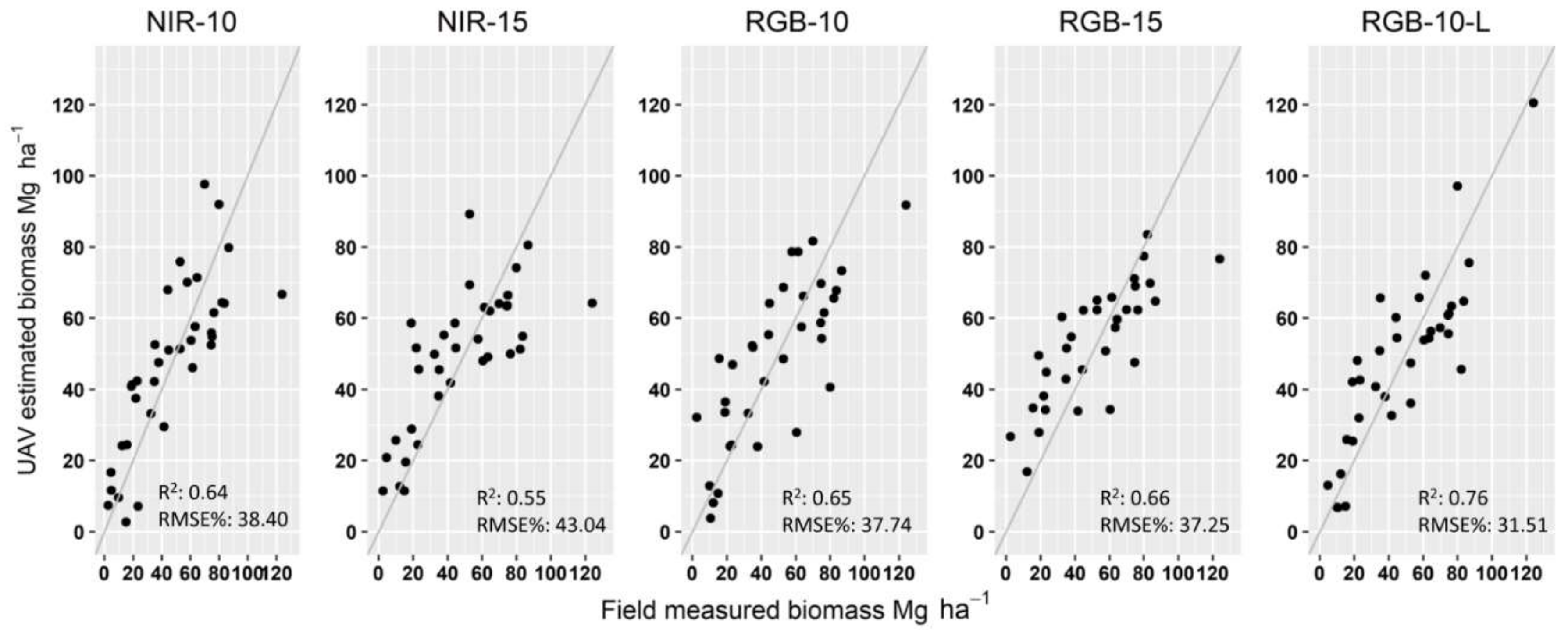
3.1. Model Accuracy after LOOCV

The biomass prediction models and their prediction accuracies are summarized in Table 4. The models had MPE values that were not significantly different from zero (p-value > 0.05). The r2 values after LOOCV ranged between 0.55 and 0.76. The RGB-10-L model yielded the best results with an RMSE% value of 31.51% while the NIR-15 model produced the largest RMSE% value of 43.04%. Models developed using the RGB camera outperformed those based on the NIR camera. The use of acquisitions with GSD 15 cm generally outperformed the ones with GSD 10 cm except for the RGB-10 acquisition, which had 0.49 RMSE% larger than RGB-15. Models developed with the RGB-10-L acquisition showed higher accuracy than RGB-10 with a side overlap of 80%.
Figure 2 presents the scatter plots of observed and predicted biomass values for each of the acquisitions using the models constructed with all the plots (see Table 4). All models had three independent variables including canopy height, canopy density and spectral variables. Furthermore, spectral variables are present in NIR-10, NIR-15, RGB-10 and RGB-15 models.

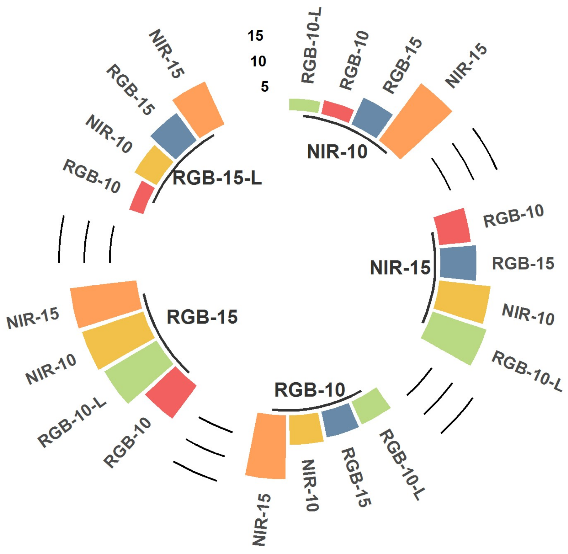
3.2. Assessment of Model Transferability

The transferability of the best fitted models, computed for each acquisition, to other acquisitions are presented in Figure 3. The application of RGB-10-L model variables to NIR-10, NIR-15, RGB-10, RGB-15 acquisitions showed the smallest differences with respect to the best fitted models for each acquisition with an average RMSE% difference of 5.97. Similar results were found when using NIR-10 model with an average RMSE% difference of 6.12. However, greater RMSE% differences were found when using RGB-10, NIR-15 and RGB-15 models with an average difference of 7.1, 8.67 and 11.48, respectively. These results show that models fitted to acquisitions with 10 cm GSD provides better results than those generated with 15 cm GSD. When considering individual acquisitions separately, NIR-15 was the most affected, with a RMSE% difference of 12.20 with respect to the best fitted models, while RGB-10 was least affected with a RMSE% difference of 5.01. The comparison between models by using ANOVA shows that there are significant differences between some of the best fitted models and the extrapolated models, with 95% probability (Figure 3). The Shapiro-Wilk test showed that the residuals were normally distributed for all models with an average p-value of 0.36. No statistically significant differences were found between acquisitions with the same GSD. No statistically significant differences were found when extrapolating NIR-10 model to RGB-10 and RGB-15 acquisitions. Similarly, no statistically significant differences were found when extrapolating RGB-10 model to RGB-15 and NIR-15, and when extrapolating RGB-10-L model to RGB-10.

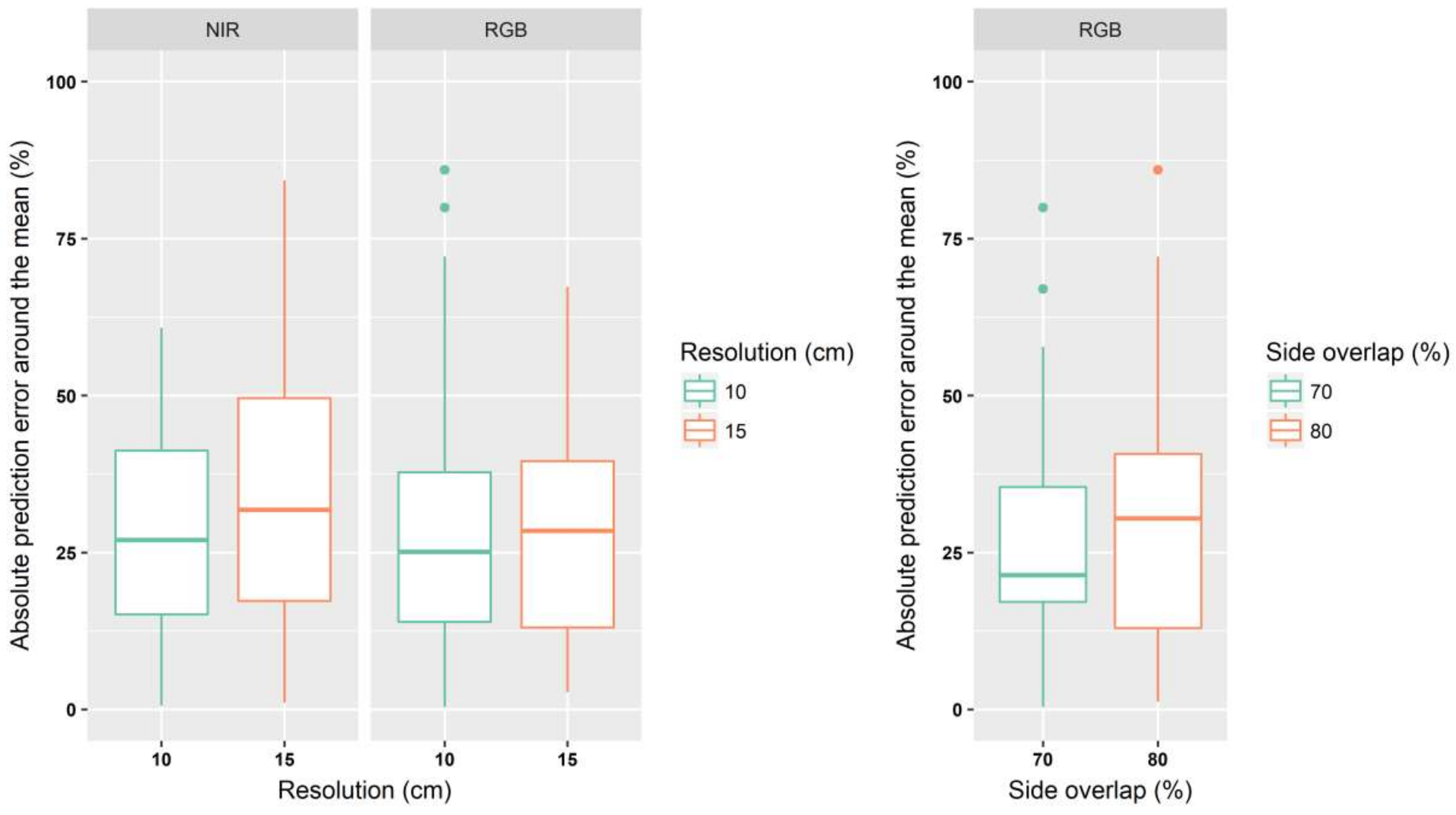
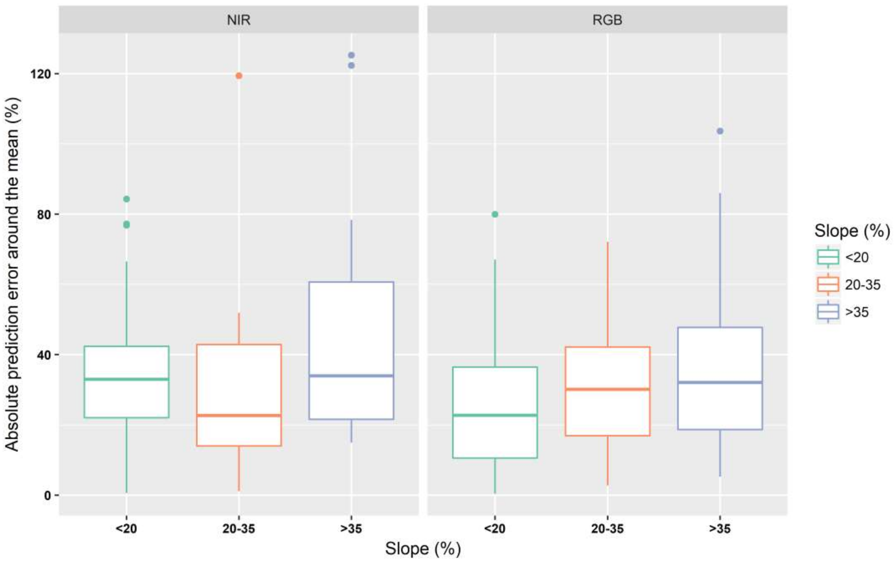
3.3. Assessment of the Influence of Flight Settings, Camera Type and Slope on Model Accuracy

The influence of image resolution, camera type and side overlap in model accuracy is graphically summarized in Figure 4 and Figure 5. Coarser resolution increases PE% values for either NIR or RGB cameras. Average increments in PE% absolute values range from 0.28 to 0.65% when using NIR or RGB, respectively. The models generated using the NIR camera, for both resolutions, present higher mean PE% errors than the RGB camera. RGB acquisition with 15 cm GSD shows a higher accuracy with an absolute PE% value of 0.5% higher than NIR 10 cm GSD. Greater dispersion of the values is found when using 80% side overlap rather than 70% and an increase of PE% was found when using 80% overlap.
The assessment of significant differences between classes shows no statistically significant differences between classes with 95% of probability. P-values for log-likelihood test were 0.83, 0.60 and 0.42 for image resolution, camera type and side overlap, respectively.
P E % = 28.26 + 0.66 · 15 c m   r e s o l u t i o n 1.73 · R G B c a m e r a + 3.47 · 80 %   s i d e   o v e r l a p
The effect of slope in biomass predictions is presented in Figure 5. The increment of terrain slope produces larger errors, especially for those plots with slopes steeper than 35%, for both RGB and NIR cameras. These slopes have greater effect when using NIR camera with a mean absolute PE% value of 48.41%. Slopes between 20 and 35% had slightly more effect when using RGB acquisitions than NIR ones. The assessment of significant differences between slope classes, performed by using a linear mixed-effects model (Equation (5)) and log-likelihood test shows that no statistically significant differences exist between classes with a p-value of 0.07.
PE% = 33.18 + 2.23·slope between 20 to 35% + 10.33·slope greater than 35%

4. Discussion

The implementation of the REDD+ mechanism for better conserving tropical dry forest and reducing carbon emissions require the integration of efficient forest inventory techniques. This study aimed at estimating biomass using different UAS flight configurations, sensors, and terrain slopes in biomass predictions within a forest reserve in miombo woodlands of Malawi. The results may be of general interest and relevance beyond the scope of this case study and might be considered for analysis in other study areas when estimating other forestry attributes.
Our results demonstrate that the data generated by UASs with different flight configurations and sensors have the potential to be successfully used in predicting biomass with RMSE% values that ranges from 31.51 to 44.66%. These values are similar to that reported by Kachamba et al. [3,22] (39.33%), developed in the same area but using a larger number of plots. Dandois et al. [43] obtained 33% of RMSE% in temperate deciduous forest and Guerra-hernández et al. [25] 11.44% and 12.59% in a Pinus pinea plantation in 2015 and 2017, respectively. Direct comparisons with the Guerra-Hernández et al. [25] study should, however, be made with caution, because the estimated RMSE% refers to single tree biomass of Pinus pinea. Furthermore, Miller et al. [21], studying monoculture plantations of the tropics, reported r2 of 0.64, similar to the results of the present study (0.55 to 0.76). The selected UAS variables in the models reflect the importance of canopy height and canopy density metrics for estimating biomass in agreement with Puliti et al. [17], Kachamba et al. [3,54], and partially with Miller et al. [21], who only included canopy height metrics. Moreover, spectral information was present in models of four out of five acquisitions highlighting the usefulness of RGB and NIR spectral bands [18].
Coarsening the image resolution from 10 to 15 cm GSD reduced model accuracy in agreement with Frey et al. [67], who showed that 8 cm GSD performed better than 16 cm GSD when analyzing DSM completeness. However, Frey et al. [67] also found that a coarser GSD of 32 cm was the most favorable for DSM reconstruction. This was explained by the effect of wind, but this result was not found when considering a voxel space. The latter is related to the estimation of forestry variables as biomass, which considers the 3D vegetation profile. Furthermore, a smaller GSD required higher forward overlap to ensure the detection of sparse trees [44,64]. Dandois et al. [43] also showed that position accuracy (X, Y) for the derived point cloud is reduced when coarsening the GSD by increasing the UAS acquisition height from 20, 40, 60 to 80 m above canopy. In contrast, Fraser et al. [44] found that 100 m flight altitude was superior to lower flight altitudes when comparing up to 120 above ground. However, those flight altitudes are not comparable to our study, with flight altitudes ranging from 286 to 430 m above ground. We were able to acquire data at much higher altitudes than commonly used, as there were no flight policy regulations in the study area. The models developed using data from the RGB camera were better than the models developed using the NIR camera. Improved model accuracy was found when using a side overlap of 70% compared to 80%. These results are in agreement with Dandois et al. [43], who stated that absolute positioning accuracy of the point cloud was unaffected by changes in photographic side overlap. However, Dandois et al. [44] found slightly better accuracy in the x, y and z coordinates when using a 60% side overlap rather than 80%. While our study did not consider the effect of wind or cloud cover, the use of a slightly lower side overlap while keeping a high forward overlap indicates that might be beneficial for SfM processing. A fixed forward overlap of 90% was kept for both cases following Dandois et al. [43], Frey et al. [67] and Torres-Sánchez et al. [45], who achieved significantly better results when using larger forward overlap values around 95%. However, the decrease of forward overlap was detected as a source of significant differences in positioning accuracy of the point cloud [43], which was considered in the present study to determine a high 90% forward overlap.
The application of the best fitted models, computed for each acquisition, to the remaining ones showed average RMSE% differences between 5.97 and 11.48. Thus, when higher canopy height variables, such as, for example Hmax or H80, are included, the models are more transferable than including lower canopy height variables or when those were not included. Furthermore, the use of models fitted to acquisitions with higher resolution provides better results when extrapolating to others acquisitions with coarser resolutions. Slightly smaller differences were also found when applying RGB than NIR with 10 cm GSD. No statistically significant differences were found between images captured by different cameras with the same GSD. Model transferability between UAS acquisitions, considering those with finer resolution and higher canopy height variables, may reduce time and cost of model parametrization as it will be possible to extrapolate a model generated for one acquisition to others [42].
The influence of image resolution, camera type and side overlap showed no statistically significant differences in the MPE% values of the models for image resolution and side overlap agreeing with Dandois et al. [43]. Furthermore, the influence of slope showed an expected pattern, the larger the terrain slope the larger the error of the models. Slopes steeper than 35% generated larger errors while slopes between 20 to 35% had slightly more effect in RGB images than NIR. However, no statistically significant differences were found between slope classes, agreeing with Ørka et al. [48], Breidenbach et al. [49] and Clark et al. [50], which were developed using ALS data. The reduction of side overlap while keeping a high forward overlap might be considered to reduce acquisition and processing time and costs.
This research has accounted for some possible effects of UAS flight configuration and post-processing, but as Dandois et al. [43] stated, there are as many combinations of acquisition settings to be considered. Thus, further analysis may focus on comparing different filtering algorithms for UAS point cloud normalization as those previously proposed by Kachamba et al. [22], those used by Miller et al. [21] or Wallace et al. [18] and the DTM-independent approach proposed by Giannetti et al. [24]. Furthermore, the effects of similar variables should be tested in other forest ecosystems including the boreal forests, in which NIR UAS cameras have been previously utilized to accurately estimate different forest structural attributes [17,68,69]. Further testing the effects of image resolution and side overlaps for estimating biomass or other forestry variables can help to increase flight efficiency and reduce post-processing time and costs. However, the reduction of forward overlap is not recommended as the lower number of images acquired during flights have been detected as an important source of error [43,45,67] and simulations using eMotion shows that there is not a significant reduction of flight time for the eBee used in the present study. As Dandois et al. [23] stated, several other effects can be analyzed related to post-processing pipelines (e.g., comparing different SfM algorithms), field data collection (i.e., number of field plot) and environmental variables (i.e., effect of aspect or slope when using different DTM approaches or the DTM-independent approach). These questions, some of which have been previously addressed using LiDAR technology, reflect that UAS is still a growing technology in forestry.

5. Conclusions

This study assesses the utility of UAS derived point clouds to estimate biomass when using different image resolution, camera types and side overlaps in Malawi miombo woodlands. The best biomass model was obtained by using an RGB camera with 10 cm GSD, and 70% side overlap and 90% forward overlap and resulted in RMSE of 14.39 Mg·ha−1. Although no statistically significant differences were found between image resolution, camera types, side overlap and terrain slope, model accuracy increased when using the RGB camera and finer image resolution while NIR camera and coarser resolution decreased model accuracy. Further studies are required to evaluate the influence of the flight and camera configurations when estimating other forest attributes as well as in other forest types. This study moves a step forward in determining optimal flight and camera types for accounting for forest biomass as assets to manage carbon emissions and reduce forest degradation in dry tropical forests.

Author Contributions

D.D. was involved in designing the research, analyzing the data and developing the manuscript. H.O.Ø. was involved in designing the research, collecting and analyzing the data as well as developing the manuscript. E.N. was involved in manuscript development. D.K. was involved in data collection and manuscript development. T.G. was involved in designing the research, analyzing the data and manuscript development.

Funding

The main author was supported by the Government of Spain, Department of Education Culture and Sports under Grant [FPU Grant BOE, 14/06250]. The fieldwork was funded by the Norwegian Government thru the Capacity Building for Managing Climate Change (CABMACC) program in Malawi.

Acknowledgments

Special thanks to the Malawi Government and the communities around the Muyobe forest reserve for granting permission to use the UAV for data collection. Thanks also to professor Trond Eid for assisting in designing the field inventory. We will also thank Herbert Jenya, Steven Mphamba, Martin Nyoni and Kola Daitoni for their support during data collection.

Conflicts of Interest

The authors declare no conflicts of interest.

References

  1. Houghton, R.A.; Byers, B.; Nassikas, A. A role for tropical forests in stabilizing atmospheric CO2. Nat. Clim. Chang. 2015, 5, 1022–1023. [Google Scholar] [CrossRef]
  2. Messinger, M.; Asner, G.; Silman, M. Rapid Assessments of Amazon Forest Structure and Biomass Using Small Unmanned Aerial Systems. Remote Sens. 2016, 8, 615. [Google Scholar] [CrossRef]
  3. Kachamba, D.; Ørka, H.; Næsset, E.; Eid, T.; Gobakken, T. Influence of Plot Size on Efficiency of Biomass Estimates in Inventories of Dry Tropical Forests Assisted by Photogrammetric Data from an Unmanned Aircraft System. Remote Sens. 2017, 9, 610. [Google Scholar] [CrossRef]
  4. Næsset, E.; Gobakken, T.; Solberg, S.; Gregoire, T.G.; Nelson, R.; Ståhl, G.; Weydahl, D. Model-assisted regional forest biomass estimation using LiDAR and InSAR as auxiliary data: A case study from a boreal forest area. Remote Sens. Environ. 2011, 115, 3599–3614. [Google Scholar] [CrossRef]
  5. Gobakken, T.; Næsset, E.; Nelson, R.; Bollandsås, O.M.; Gregoire, T.G.; Ståhl, G.; Holm, S.; Ørka, H.O.; Astrup, R. Estimating biomass in Hedmark County, Norway using national forest inventory field plots and airborne laser scanning. Remote Sens. Environ. 2012, 123, 443–456. [Google Scholar] [CrossRef]
  6. Su, Y.; Guo, Q.; Xue, B.; Hu, T.; Alvarez, O.; Tao, S.; Fang, J. Spatial distribution of forest aboveground biomass in China: Estimation through combination of spaceborne lidar, optical imagery, and forest inventory data. Remote Sens. Environ. 2016, 173, 187–199. [Google Scholar] [CrossRef]
  7. McRoberts, R.; Tomppo, E. Remote sensing support for national forest inventories. Remote Sens. Environ. 2007, 110, 412–419. [Google Scholar] [CrossRef]
  8. Deo, R.; Russell, M.; Domke, G.; Andersen, H.-E.; Cohen, W.; Woodall, C. Evaluating Site-Specific and Generic Spatial Models of Aboveground Forest Biomass Based on Landsat Time-Series and LiDAR Strip Samples in the Eastern USA. Remote Sens. 2017, 9, 598. [Google Scholar] [CrossRef]
  9. Matasci, G.; Hermosilla, T.; Wulder, M.A.; White, J.C.; Coops, N.C.; Hobart, G.W.; Zald, H.S.J. Large-area mapping of Canadian boreal forest cover, height, biomass and other structural attributes using Landsat composites and lidar plots. Remote Sens. Environ. 2018, 209, 90–106. [Google Scholar] [CrossRef]
  10. Dalponte, M.; Frizzera, L.; Ørka, H.O.; Gobakken, T.; Næsset, E.; Gianelle, D. Predicting stem diameters and aboveground biomass of individual trees using remote sensing data. Ecol. Indic. 2018, 85, 367–376. [Google Scholar] [CrossRef]
  11. Skowronski, N.S.; Clark, K.L.; Gallagher, M.; Birdsey, R.A.; Hom, J.L. Airborne laser scanner-assisted estimation of aboveground biomass change in a temperate oak–pine forest. Remote Sens. Environ. 2014, 151, 166–174. [Google Scholar] [CrossRef]
  12. Domingo, D.; Lamelas, M.; Montealegre, A.; García-Martín, A.; de la Riva, J. Estimation of Total Biomass in Aleppo Pine Forest Stands Applying Parametric and Nonparametric Methods to Low-Density Airborne Laser Scanning Data. Forests 2018, 9, 158. [Google Scholar] [CrossRef]
  13. Mauya, E.W.; Hansen, E.H.; Gobakken, T.; Bollandsås, O.M.; Malimbwi, R.E.; Næsset, E. Effects of field plot size on prediction accuracy of aboveground biomass in airborne laser scanning-assisted inventories in tropical rain forests of Tanzania. Carbon Balance Manag. 2015, 10, 10. [Google Scholar] [CrossRef]
  14. Remondino, F.; Spera, M.G.; Nocerino, E.; Menna, F.; Nex, F. State of the art in high density image matching. Photogramm. Rec. 2014, 29, 144–166. [Google Scholar] [CrossRef]
  15. Sankey, T.; Donager, J.; McVay, J.; Sankey, J.B. UAV lidar and hyperspectral fusion for forest monitoring in the southwestern USA. Remote Sens. Environ. 2017. [Google Scholar] [CrossRef]
  16. Shin, P.; Sankey, T.; Moore, M.; Thode, A.; Shin, P.; Sankey, T.; Moore, M.M.; Thode, A.E. Evaluating Unmanned Aerial Vehicle Images for Estimating Forest Canopy Fuels in a Ponderosa Pine Stand. Remote Sens. 2018, 10, 1266. [Google Scholar] [CrossRef]
  17. Puliti, S.; Olerka, H.; Gobakken, T.; Næsset, E. Inventory of Small Forest Areas Using an Unmanned Aerial System. Remote Sens. 2015, 7, 9632–9654. [Google Scholar] [CrossRef]
  18. Wallace, L.; Lucieer, A.; Malenovský, Z.; Turner, D.; Vopěnka, P. Assessment of Forest Structure Using Two UAV Techniques: A Comparison of Airborne Laser Scanning and Structure from Motion (SfM) Point Clouds. Forests 2016, 7, 62. [Google Scholar] [CrossRef]
  19. Tuominen, S.; Balazs, A.; Saari, H.; Pölönen, I.; Sarkeala, J.; Viitala, R. Unmanned aerial system imagery and photogrammetric canopy height data in area-based estimation of forest variables. Silva Fenn. 2015, 49. [Google Scholar] [CrossRef]
  20. Lisein, J.; Pierrot-Deseilligny, M.; Bonnet, S.; Lejeune, P. A Photogrammetric Workflow for the Creation of a Forest Canopy Height Model from Small Unmanned Aerial System Imagery. Forests 2013, 4, 922–944. [Google Scholar] [CrossRef]
  21. Miller, E.; Dandois, J.; Detto, M.; Hall, J. Drones as a Tool for Monoculture Plantation Assessment in the Steepland Tropics. Forests 2017, 8, 168. [Google Scholar] [CrossRef]
  22. Kachamba, D.; Ørka, H.; Gobakken, T.; Eid, T.; Mwase, W. Biomass Estimation Using 3D Data from Unmanned Aerial Vehicle Imagery in a Tropical Woodland. Remote Sens. 2016, 8, 968. [Google Scholar] [CrossRef]
  23. Dandois, J.P.; Ellis, E.C. High spatial resolution three-dimensional mapping of vegetation spectral dynamics using computer vision. Remote Sens. Environ. 2013, 136, 259–276. [Google Scholar] [CrossRef]
  24. Giannetti, F.; Chirici, G.; Gobakken, T.; Næsset, E.; Travaglini, D.; Puliti, S. A new approach with DTM-independent metrics for forest growing stock prediction using UAV photogrammetric data. Remote Sens. Environ. 2018, 213, 195–205. [Google Scholar] [CrossRef]
  25. Guerra-Hernández, J.; González-Ferreiro, E.; Monleón, V.; Faias, S.; Tomé, M.; Díaz-Varela, R. Use of Multi-Temporal UAV-Derived Imagery for Estimating Individual Tree Growth in Pinus pinea Stands. Forests 2017, 8, 300. [Google Scholar] [CrossRef]
  26. Dempewolf, J.; Nagol, J.; Hein, S.; Thiel, C.; Zimmermann, R. Measurement of Within-Season Tree Height Growth in a Mixed Forest Stand Using UAV Imagery. Forests 2017, 8, 231. [Google Scholar] [CrossRef]
  27. Guerra-Hernández, J.; Cosenza, D.N.; Rodriguez, L.C.E.; Silva, M.; Tomé, M.; Díaz-Varela, R.A.; González-Ferreiro, E. Comparison of ALS- and UAV(SfM)-derived high-density point clouds for individual tree detection in Eucalyptus plantations. Int. J. Remote Sens. 2018, 39, 5211–5235. [Google Scholar] [CrossRef]
  28. Mohan, M.; Silva, C.; Klauberg, C.; Jat, P.; Catts, G.; Cardil, A.; Hudak, A.; Dia, M. Individual Tree Detection from Unmanned Aerial Vehicle (UAV) Derived Canopy Height Model in an Open Canopy Mixed Conifer Forest. Forests 2017, 8, 340. [Google Scholar] [CrossRef]
  29. Wallace, L.; Lucieer, A.; Watson, C.S. Evaluating Tree Detection and Segmentation Routines on Very High Resolution UAV LiDAR Data. IEEE Trans. Geosci. Remote Sens. 2014, 52, 7619–7628. [Google Scholar] [CrossRef]
  30. Saarela, S.; Grafström, A.; Ståhl, G.; Kangas, A.; Holopainen, M.; Tuominen, S.; Nordkvist, K.; Hyyppä, J. Model-assisted estimation of growing stock volume using different combinations of LiDAR and Landsat data as auxiliary information. Remote Sens. Environ. 2015, 158, 431–440. [Google Scholar] [CrossRef]
  31. Chianucci, F.; Disperati, L.; Guzzi, D.; Bianchini, D.; Nardino, V.; Lastri, C.; Rindinella, A.; Corona, P. Estimation of canopy attributes in beech forests using true colour digital images from a small fixed-wing UAV. Int. J. Appl. Earth Obs. Geoinf. 2016, 47, 60–68. [Google Scholar] [CrossRef]
  32. Wallace, L. Assessing the stability of canopy maps produced from UAV-LiDAR data. In Proceedings of the 2013 IEEE International Geoscience and Remote Sensing Symposium—IGARSS, Melbourne, VIC, Australia, 21–26 July 2013; pp. 3879–3882. [Google Scholar]
  33. Bagaram, M.; Giuliarelli, D.; Chirici, G.; Giannetti, F.; Barbati, A. UAV Remote Sensing for Biodiversity Monitoring: Are Forest Canopy Gaps Good Covariates? Remote Sens. 2018, 10, 1397. [Google Scholar] [CrossRef]
  34. Getzin, S.; Nuske, R.; Wiegand, K. Using Unmanned Aerial Vehicles (UAV) to Quantify Spatial Gap Patterns in Forests. Remote Sens. 2014, 6, 6988–7004. [Google Scholar] [CrossRef]
  35. Puliti, S.; Talbot, B.; Astrup, R.; Puliti, S.; Talbot, B.; Astrup, R. Tree-Stump Detection, Segmentation, Classification, and Measurement Using Unmanned Aerial Vehicle (UAV) Imagery. Forests 2018, 9, 102. [Google Scholar] [CrossRef]
  36. Fleishman, E.; Yen, J.D.L.; Thomson, J.R.; Mac Nally, R.; Dobkin, D.S.; Leu, M. Identifying spatially and temporally transferrable surrogate measures of species richness. Ecol. Indic. 2018, 84, 470–478. [Google Scholar] [CrossRef]
  37. Fekety, P.A.; Falkowski, M.J.; Hudak, A.T. Temporal transferability of LiDAR-based imputation of forest inventory attributes. Can. J. For. Res. 2015, 45, 422–435. [Google Scholar] [CrossRef]
  38. Zhao, K.; Suarez, J.C.; Garcia, M.; Hu, T.; Wang, C.; Londo, A. Utility of multitemporal lidar for forest and carbon monitoring: Tree growth, biomass dynamics, and carbon flux. Remote Sens. Environ. 2018, 204, 883–897. [Google Scholar] [CrossRef]
  39. Cao, L.; Coops, N.C.; Innes, J.L.; Sheppard, S.R.J.; Fu, L.; Ruan, H.; She, G. Estimation of forest biomass dynamics in subtropical forests using multi-temporal airborne LiDAR data. Remote Sens. Environ. 2016, 178, 158–171. [Google Scholar] [CrossRef]
  40. Meyer, V.; Saatchi, S.S.; Chave, J.; Dalling, J.W.; Bohlman, S.; Fricker, G.A.; Robinson, C.; Neumann, M.; Hubbell, S. Detecting tropical forest biomass dynamics from repeated airborne lidar measurements. Biogeosciences 2013, 10, 5421–5438. [Google Scholar] [CrossRef]
  41. Bollandsås, O.M.; Gregoire, T.G.; Næsset, E.; Øyen, B.H. Detection of biomass change in a Norwegian mountain forest area using small footprint airborne laser scanner data. Stat. Methods Appl. 2013, 22, 113–129. [Google Scholar] [CrossRef]
  42. Noordermeer, L.; Bollandsås, O.M.; Gobakken, T.; Næsset, E. Direct and indirect site index determination for Norway spruce and Scots pine using bitemporal airborne laser scanner data. For. Ecol. Manag. 2018, 428, 104–114. [Google Scholar] [CrossRef]
  43. Dandois, J.; Olano, M.; Ellis, E. Optimal Altitude, Overlap, and Weather Conditions for Computer Vision UAV Estimates of Forest Structure. Remote Sens. 2015, 7, 13895–13920. [Google Scholar] [CrossRef]
  44. Fraser, B.; Congalton, R.; Fraser, B.T.; Congalton, R.G. Issues in Unmanned Aerial Systems (UAS) Data Collection of Complex Forest Environments. Remote Sens. 2018, 10, 908. [Google Scholar] [CrossRef]
  45. Torres-Sánchez, J.; López-Granados, F.; Borra-Serrano, I.; Peña, J.M. Assessing UAV-collected image overlap influence on computation time and digital surface model accuracy in olive orchards. Precis. Agric. 2018, 19, 115–133. [Google Scholar] [CrossRef]
  46. Ni, W.; Sun, G.; Pang, Y.; Zhang, Z.; Liu, J.; Yang, A.; Wang, Y.; Zhang, D. Mapping Three-Dimensional Structures of Forest Canopy Using UAV Stereo Imagery: Evaluating Impacts of Forward Overlaps and Image Resolutions With LiDAR Data as Reference. IEEE J. Sel. Top. Appl. Earth Obs. Remote Sens. 2018, 11, 3578–3589. [Google Scholar] [CrossRef]
  47. Montealegre, A.; Lamelas, M.; Riva, J. Interpolation Routines Assessment in ALS-Derived Digital Elevation Models for Forestry Applications. Remote Sens. 2015, 7, 8631–8654. [Google Scholar] [CrossRef]
  48. Ørka, H.O.; Bollandsås, O.M.; Hansen, E.H.; Næsset, E.; Gobakken, T. Effects of terrain slope and aspect on the error of ALS-based predictions of forest attributes. For. An Int. J. For. Res. 2018, 91, 225–237. [Google Scholar] [CrossRef]
  49. Breidenbach, J.; Koch, B.; Kändler, G.; Kleusberg, A. Quantifying the influence of slope, aspect, crown shape and stem density on the estimation of tree height at plot level using lidar and InSAR data. Int. J. Remote Sens. 2008, 29, 1511–1536. [Google Scholar] [CrossRef]
  50. Clark, M.L.; Clark, D.B.; Roberts, D.A. Small-footprint lidar estimation of sub-canopy elevation and tree height in a tropical rain forest landscape. Remote Sens. Environ. 2004, 91, 68–89. [Google Scholar] [CrossRef]
  51. Khosravipour, A.; Skidmore, A.K.; Wang, T.; Isenburg, M.; Khoshelham, K. Effect of slope on treetop detection using a LiDAR Canopy Height Model. ISPRS J. Photogramm. Remote Sens. 2015, 104, 44–52. [Google Scholar] [CrossRef]
  52. Kouba, J. A guide to using International GNSS Service (IGS) products. Int. GNSS 2009, 6, 34. [Google Scholar] [CrossRef]
  53. Takasu, T. RTKLIB 2.4.2 Manual. Available online: www.rtklib.com/prog/manual_2.4.2.pdf (accessed on 1 April 2019).
  54. Kachamba, D.J.; Eid, T. Total tree, merchantable stem and branch volume models for miombo woodlands of Malawi. South. For. J. For. Sci. 2016, 78, 41–51. [Google Scholar] [CrossRef]
  55. SENSEFLY EBEE RTK Extended User Manual (Page 7 of 190). Available online: https://www.manualslib.com/manual/1255561/Sensefly-Ebee-Rtk.html?page=7#manual (accessed on 14 November 2018).
  56. Agisoft LLC. Agisoft PhotoScan User Manual, Prof. Ed. Version 0.9.0; Agisoft LLC.: St. Petersburg, Russia, 2016. [Google Scholar] [CrossRef]
  57. Axelsson, P. Processing of laser scanner data—Algorithms and applications. ISPRS J. Photogramm. Remote Sens. 1999, 54, 138–147. [Google Scholar] [CrossRef]
  58. Maneewongvatana, S.; Mount, D.M. Analysis of approximate nearest neighbor searching with clustered point sets. In Data Structures, Near Neighbor Searches, and Methodology: Fifth and Sixth DIMACS Implementation Challenges; American Mathematical Society: Providence, RI, USA, 1999. [Google Scholar] [CrossRef]
  59. scipy.spatial.KDTree—SciPy v0.14.0 Reference Guide. Available online: https://docs.scipy.org/doc/scipy-0.14.0/reference/generated/scipy.spatial.KDTree.html (accessed on 15 November 2018).
  60. Wallace, L.; Bellman, C.; Hally, B.; Hernandez, J.; Jones, S.; Hillman, S. Assessing the Ability of Image Based Point Clouds Captured from a UAV to Measure the Terrain in the Presence of Canopy Cover. Forests 2019, 10, 284. [Google Scholar] [CrossRef]
  61. Næsset, E. Practical large-scale forest stand inventory using a small-footprint airborne scanning laser. Scand. J. For. Res. 2004, 19, 164–179. [Google Scholar] [CrossRef]
  62. McGaughey, R. FUSION/LDV: Software for LIDAR Data Analysis and Visualization 2009. Available online: https://w3.ual.es/GruposInv/ProyectoCostas/FUSION_manual.pdf (accessed on 21 February 2019).
  63. Meng, J.; Li, S.; Wang, W.; Liu, Q.; Xie, S.; Ma, W. Mapping Forest Health Using Spectral and Textural Information Extracted from SPOT-5 Satellite Images. Remote Sens. 2016, 8, 719. [Google Scholar] [CrossRef]
  64. Maltamo, M.; Næsset, E.; Vauhkonen, J. Forestry Applications of Airborne Laser Scanning: Concepts and Case Studies; Maltamo, M., Næsset, E., Vauhkonen, J., Eds.; Managing Forest Ecosystems; Springer: Dordrecht, The Netherlands, 2014; Volume 27, ISBN 978-94-017-8662-1. [Google Scholar]
  65. Andersen, H.-E.; McGaughey, R.J.; Reutebuch, S.E. Estimating forest canopy fuel parameters using LIDAR data. Remote Sens. Environ. 2005, 94, 441–449. [Google Scholar] [CrossRef]
  66. Laird, N.M.; Ware, J.H. Random-Effects Models for Longitudinal Data. Biometrics 1982, 38, 963. [Google Scholar] [CrossRef]
  67. Frey, J.; Kovach, K.; Stemmler, S.; Koch, B. UAV Photogrammetry of Forests as a Vulnerable Process. A Sensitivity Analysis for a Structure from Motion RGB-Image Pipeline. Remote Sens. 2018, 10, 912. [Google Scholar] [CrossRef]
  68. Puliti, S.; Saarela, S.; Gobakken, T.; Ståhl, G.; Næsset, E. Combining UAV and Sentinel-2 auxiliary data for forest growing stock volume estimation through hierarchical model-based inference. Remote Sens. Environ. 2017. [Google Scholar] [CrossRef]
  69. Puliti, S.; Gobakken, T.; Ørka, H.O.; Næsset, E. Assessing 3D point clouds from aerial photographs for species-specific forest inventories. Scand. J. For. Res. 2017, 32, 68–79. [Google Scholar] [CrossRef]
Figure 1. Study area location in Malawi (left) and distribution of the 37 field inventory plots (right). The orthophoto was derived from a UAS flight with an RGB-10 camera (Table 1).
Remotesensing 11 00948 g001
Figure 2. Scatterplots of predicted vs. ground reference values of biomass (Mg·ha−1) for the different acquisitions. The suffix 10 refers to GSD 10 cm. The suffix 15 refers to GSD 15 cm. RGB-10-L acquisition was performed with GSD 10 cm and side overlap of 70%.
Remotesensing 11 00948 g002
Figure 3. Differences in RMSE% between the best fitted model for each acquisition and other acquisitions using the same UAS variables. Significant differences from ANOVA test are indicated with: *** for 0.001; ** for 0.01 and * for 0.05.
Remotesensing 11 00948 g003
Figure 4. Differences between image resolution, camera type and side overlap effects in biomass predictions.
Remotesensing 11 00948 g004
Figure 5. Slope effect in biomass predictions. The mean prediction error per class is included using red dots in the boxplots. The biomass prediction accuracies are not significantly different among the slope classes.
Remotesensing 11 00948 g005
Table 1. Summary of the field plot characteristics (n = 37).
CharacteristicRangeMeanStd 1Cv 2
Biomass (Mg·ha−1)2.48–123.9445.6829.5464.66
Basal area (m2·ha−1)0.62–16.106.523.8258.58
Number of stems (ha−1)10–83042016339
Lorey’s mean height (m)4.19–14.586.361.7427.43
1 Std = Standard deviation, 2 Cv = Coefficient of variation.
Table 2. Summary of the flight characteristics for each acquisition. The prefix of the abbreviations refers to camera type (NIR and RGB, respectively), the first suffix refers to GSD (10 and 15 cm, respectively) and the second suffix refers to side overlap (L is 70% side overlap). NIR-10 was performed with GSD 10 cm; NIR-15 was performed with GSD 15 cm; RGB-10 was performed with GSD 10 cm; RGB-15 was performed with GSD 15 cm; RGB-10-L was performed with GSD 10 cm and side overlap of 70%.
AcquisitionDate
(day-month-year)
Side Overlap (%)Flight Height (m)Resolution (cm)Number of FlightsNumber of ImagesFlight Time (min)Wind Speed (m·s−1)Cloud Cover (%)
NIR-1025-04-1580286102470616–8.520
NIR-1526-04-1580430152300414–650–90
RGB-1023-04-15 to 25-04-158032510916912065–8.820–100
RGB-1526-04-1580487152237384–570–100
RGB-10-L26-04-1570325103370514–630–60
Table 3. Processing steps and parameter settings used in Agisoft Photoscan Professional software for 3D point generation using UAS imagery.
TaskParameters
(i)
Image alignment
Accuracy: high
Pair selection: reference
Key points: 40,000
Tie points: 1000
(ii)
Guided marker positioning
Manual relocation of markers on the 11 GCPs for all the photos where a GCP was visible.
(iii)
Building dense point clouds
Quality: medium
Depth filtering: mild
Table 4. Summary of the models for each acquisition after applying LOOCV. The suffix 10 refers to GSD 10 cm. The suffix 15 refers to GSD 15 cm. RGB-10-L acquisition was performed with GSD 10 cm and side overlap of 70%.
AcquisitionUAS Variablesr2 *RMSE%MPE%p-Value
NIR-10Hmax, D1, S70.red0.6438.40−0.510.94
NIR-15D1, Ssd.red, Sskewness.green0.5543.040.031.00
RGB-10Hvariance, D1, S40.red0.6537.740.100.99
RGB-15H30, D2, S10.green0.6637.250.670.91
RGB-10-LH80, D2, Hskewness0.7631.510.021.00
* Pearson’s linear correlation coefficient.

