Abstract
Point clouds obtained from laser scanning techniques are now a standard type of spatial data for characterising terrain surfaces. Some have been shared as open data for free access. A problem with the use of these free point cloud data is that the data density may be more than necessary for a given application, leading to higher computational cost in subsequent data processing and visualisation. In such cases, to make the dense point clouds more manageable, their data density can be reduced. This research proposes a new coarse-to-fine sub-sampling method for reducing point cloud data density, which honours the local surface complexity of a terrain surface. The method proposed is tested using four point clouds representing terrain surfaces with distinct spatial characteristics. The effectiveness of the iterative coarse-to-fine method is evaluated and compared against several benchmarks in the form of typical sub-sampling methods available in open source software for point cloud processing.
1. Introduction
In recent years, free access to an increasing number of LiDAR (i.e., Light detection and ranging) databases (e.g., the OpenTopography Facility of US and the LiDAR databases from The Environment Agency of the UK) is available to promote the use of LiDAR point clouds. During laser scanning campaigns, the spatial resolution of data acquisition does not often take into account the spatial variation in the surface complexity. In addition, some local areas may be measured multiple times from different stations or flight paths. Consequently, oversampling may occur in some areas and can lead to a large volume of point cloud data, which is more than required for a given application [1,2,3]. This is more likely to be the case for use of open LiDAR data where users have no control on the spatial resolution of data acquisition. In those cases, to make the dataset more manageable and fit for purpose, a thinned point cloud can be sub-sampled from the original point cloud [4,5]. For applications of LiDAR point clouds in Earth science, this may be achieved by selecting a subset of the original point cloud (i.e., the subset selected is the thinned point cloud) or by removing a set of data points from the original dataset (i.e., the remaining data points constitute the thinned point cloud). In either case, the coordinates of individual data points are not altered during the process of thinning from the original point cloud to the reduced one.
The typical sub-sampling methods available in point cloud processing software (e.g., CloudCompare) for data thinning include the random, minimal distance and uniform methods. The random method is the simplest for reducing data density, in which a specified number of data points is selected in a random manner [6,7]. In the minimal distance method, the data point selection is constrained by a minimum distance so that no data point in the selected subset is closer to another data point than the minimum distance specified. In the uniform method, a voxel structure is created and the data point closest to the centre of each voxel is selected. The latter two methods can achieve a more homogeneous spatial distribution of data points in the point cloud of reduced data density [8]. The average data spacing is determined by the minimal distance or the voxel edge length specified. Although these methods are computationally efficient, none of these methods honour the spatial variation of the terrain surface complexity.
From theoretical [9,10,11] and empirical studies [12,13,14,15] on the relation between terrain model accuracy and the density of data points used to build the model, it is widely known that more data points are required to represent local areas where the terrain surface is more complex for a given modelling accuracy requirement (typically, digital elevation model accuracy). To this end, the relative importance of data points needs to be evaluated so that key points are preserved while less important points are removed in the data thinning process [4,5].
A survey of the typical methods for selecting key points was carried out by Heckbert and Garland [16]. Amongst those methods, the point-additive method [5,17,18,19,20] and the point-subtractive method [18,21,22] are considered suitable and effective methods for scattered point cloud data representing a terrain surface. In the iterative addition method, some initial key points (e.g., local highest or lowest data points [5]) are selected and used to generate a triangulated irregular network (TIN) surface. The deviation of each candidate data point to the TIN surface is calculated globally or locally, and the data point of the largest deviation is classified as a new key point and is added to the key point dataset. The updated key point dataset is used to generate a new TIN surface for selecting the next key point(s). This iterative process continues until a predefined number of data points or a threshold deviation is reached. The point-subtractive method is the reverse of the point-additive method, and starts with a TIN surface based on all candidate data points available. It iteratively removes one or several data points until a predefined number of data points or a threshold error is reached. Although these two types of methods are effective in producing a thinned point cloud with a data density that varies with the terrain surface complexity, such methods often have a high computational cost [5,16,22] because they need to sweep through each and every candidate data point. In addition to the aforementioned methods, sub-sampling with local adaptation to surface roughness can also be achieved using a non-stationary geostatistical approach [23,24,25]. However, this approach requires the production and interpretation of local variograms, which is a time-consuming process and impractical to be applied in practice. A deep learning method for optimised point cloud sampling was also attempted, however it may lead to a thinned point cloud that is not guaranteed to be a subset of the original one [26].
In this research, a spatially non-stationary data sampling method that honours the local surface complexity of a terrain surface was investigated. A new coarse-to-fine resolution method was demonstrated and tested using four LiDAR point clouds that represent bare terrain surfaces of different characteristics. The typical sub-sampling methods were also implemented as benchmarks and compared to the proposed method.
2. Methods
2.1. The Coarse-to-Fine Method
The coarse-to-fine method involves an iterative process for sub-sampling from a point cloud, and it includes the following steps (the key steps are also shown in Figure 1). In Step 1, the whole area is partitioned into a set of local sub-areas. In Step 2, regular grid locations over the whole area are defined and allocated to each individual sub-area. In other words, a total number of grid locations (i.e., ) surrounded by the kth local sub-area are allocated to the sub-area . In Step 3, the original point cloud is used to predict the elevation values () at all the grid locations . In Step 4, a subset point cloud is produced using homogeneous voxel cubes (of edge length ) where the data point closest to the centre of each voxel is selected. The method starts with a large edge length S1 and hence a coarse-resolution subset point cloud. In Step 5, the subset point cloud is used to predict the elevation values () at all the grid locations . The elevation differences are calculated and can be readily allocated to each individual sub-area (i.e., based on the allocation of the grid locations in Step 2). These lead to local elevation differences , where and represent the predicted elevations of the ith () grid location within the kth sub-area using the subset point cloud and the original point cloud, respectively. The values are then used to calculate the local metric (i.e., root mean square error) for each individual sub-area using the following equation.
where represents the number of grid locations in the kth sub-area, represents the difference between the predicted elevations of the ith grid location within the kth sub-area using the subset point cloud and the original point cloud, respectively.
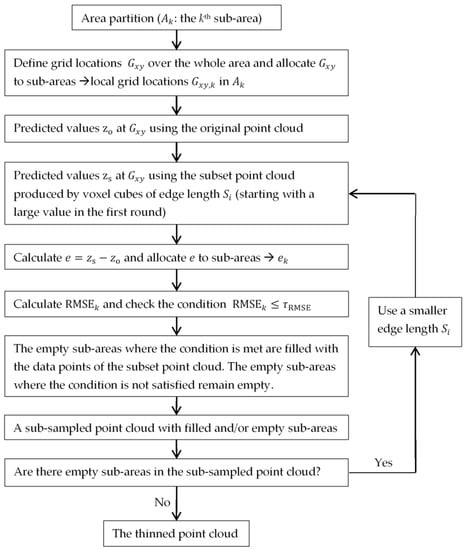
Figure 1.
The key steps involved in the coarse-to-fine method.
In Step 6, the following condition is checked: a predefined threshold . For the sub-areas where the condition is met, the data points (of the subset point cloud) surrounded by those sub-areas are kept. The other sub-areas where the condition is not satisfied are left empty. Step 6 leads to a sub-sampled point cloud with a combination of filled and empty sub-areas. To fill all empty sub-areas with data points, Steps 4–6 are iterated. In each subsequent iteration, a smaller edge length for the voxel cubes is used, leading to a subset of higher data density. However, the same threshold RMSE is used in all iterations.
The logic underpinning the aforementioned steps is described in the following. The local is an indicator for the complexity of local spatial variation. If a local value exceeds the pre-defined threshold, it indicates that the spatial variation in the local area is more complex than that the threshold RMSE represents. Therefore, more data points are required to preserve the local surface characteristics. This is achieved by reducing the voxel size.
2.2. Other Typical Methods for Comparison
Several other typical methods (i.e., the random method, the uniform method and the minimal distance method) are also considered for comparison. Detailed descriptions of these methods can be found in the Introduction.
To evaluate the effectiveness of the methods considered, the thinned point clouds obtained using each method are compared to the original point cloud by interpolation to a total number of N grid locations distributed regularly over the whole area, which leads to the error representing the difference between the interpolated values derived using the thinned and the original point clouds at the jth grid location. The values () at all the grid locations are used to calculate several global metrics, including RMSE, mean error (), standard error (), and maximum deviation (i.e., the maximum value of ). Amongst these statistical metrics, the global RMSE is considered the main metric for evaluating the effectiveness of each method and is widely adopted in the relevant literature [4,5].
3. Study Data
The study datasets considered in this research comprise four airborne LiDAR point clouds. These datasets represent a mix of bare terrain surfaces of distinct characteristics: a hilly and relatively rough surface (Figure 2a), a hilly and relatively smooth surface (Figure 2b), a comparatively flat and rough surface (Figure 2c), and a flat and smooth surface (Figure 2d). The point clouds considered consist of 297,550 (hilly rough), 270,342 (hilly smooth), 307,706 (flat rough), and 69,492 (flat smooth) bare ground data points over an area of approximately 350 m by 350 m. These LiDAR datasets come from a large LiDAR dataset acquired at a volcanic field in Central Nevada, by the National Centre for Airborne Laser Mapping, USA.
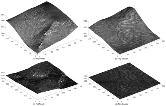
Figure 2.
The light detection and ranging (LiDAR) point cloud datasets investigated.
4. Analysis and Results
4.1. An Example for the Coarse-to-Fine Method
The data processing was carried out in MATLAB. To implement the coarse-to-fine method, an example is presented where specific values of the parameters involved were used. A simple approach for area partition was used, in which the whole area was divided into square sub-areas (e.g., 20 × 20 = 400 square sub-areas) of the same edge length over the whole area. A grid resolution of 1 m was used for the calculation of . The grid resolution should be fine enough (compared to the size of individual sub-areas) so that an adequate number of is available for calculating the local . For prediction to the grid locations, the TIN with linear interpolation was used. An initial edge length (e.g., Si = 8 m) for the voxel edge length was used. In the following iterations, the edge length Si was gradually reduced at an equal decreasing interval (e.g., 0.2 m). The ending edge length depends on a user-specified threshold RMSE.
To show a sub-sampled point cloud using the coarse-to-fine method, an example is presented using the point cloud representing the hilly rough surface and a user-specified threshold RMSE of 0.085 m. The values of the parameters applied were those reported in the previous paragraph. The original and the sub-sampled point clouds are shown in Figure 3a,b, respectively. The sub-sampled point cloud consists of 67,457 data points (approximately 22.67% of the original dataset), and its spatial variation in data density is obvious. For the MATLAB (2017a version) codes used, the time taken for the subsampling was approximately 58 seconds using an average office computer (4 cores of i5-3470 CPU @ 3.2 GHz and 8 GB RAM).
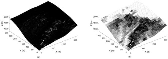
Figure 3.
The hilly rough terrain surface: (a) the original point cloud, (b) the sub-sampled point cloud obtained using the coarse-to-fine method (20 × 20 = 400 sub-areas, the threshold root mean square error (RMSE) = 0.085 m).
It is expected that more data points should be selected in sub-areas where the surface is more complex. To confirm this, a local surface roughness map was produced using the local root mean square height (RMSH) method, which is a roughness metric applied widely in Earth Science [27,28]. The window size used for calculating the RMSH was the same as that for the individual sub-areas for data sampling. The local surface roughness (shown in Figure 4b) has an evident correlation with the local data density (in Figure 4a).
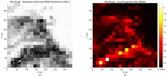
Figure 4.
The hilly rough terrain surface: (a) the sub-sampled point cloud obtained using the coarse-to-fine method (20 × 20 = 400 sub-areas, the threshold RMSE = 0.085 m), (b) the local surface roughness root mean square height (RMSH).
4.2. Comparison on Effectiveness
The commonly used methods and the coarse-to-fine method were implemented for the four LiDAR datasets considered. The original point clouds were reduced to lower data densities of various levels (represented by the number of data points selected). The level of reduction ranges from approximately 4% to 80% of the original point clouds.
The thinned point clouds were compared to the original point cloud at a grid resolution of 1 m. The statistical metrics introduced in Section 2.2 were calculated. For a more direct comparison, the parameters for the minimal distance method and the uniform method were determined using a trial-and-error approach so that the number of data points selected using these two methods were approximately the same as those selected using the coarse-to-fine method. For the random method, multiple rounds (i.e., 20 in this study) of random data selection were performed, and the results were averaged over all rounds to produce the mean values of the metrics considered.
The results in terms of RMSE are shown in Figure 5. It is expected that the RMSE decreased with increasing data density for the sub-sampling methods and the terrain surfaces investigated. The random method produced the lowest accuracy for all the datasets considered. Similar accuracy (higher than that of the random method) was observed for the minimal distance method and the uniform method, suggesting that evenly distributed data points lead to smaller differences from the original point cloud than a random distribution. The coarse-to-fine method performs more effectively than the other methods that do not honour the spatial variation of the terrain surface characteristics.
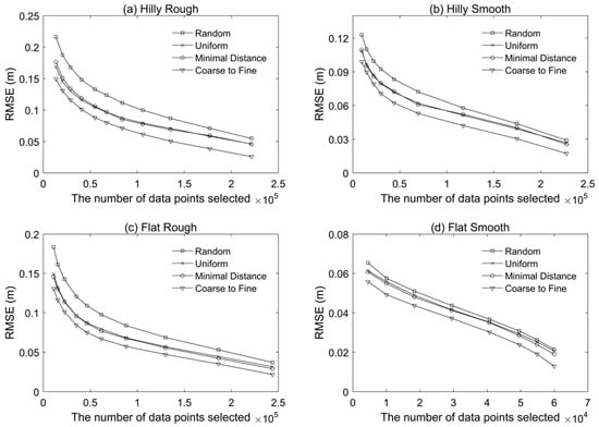
Figure 5.
The RMSE versus the number of data points of thinned point clouds for the four terrain surfaces: (a) hilly rough, (b) hilly smooth, (c) flat rough, and (d) flat smooth.
Figure 6 shows very small mean errors as compared to the corresponding RMSE, suggesting that systematic (or biased) deviations of the thinned point clouds from the original point clouds were minimal for all the sub-sampling methods considered. It was also observed that a more complex surface was likely to result in a larger mean error (e.g., Hilly Rough versus Flat Smooth). The standard errors are shown in Figure 7, which illustrates the methods had similar results to those based on the RMSE metric. This is expected as the mean errors were all comparatively small. Figure 8 shows the maximum elevation difference between the thinned point cloud and the original point at the pre-defined grid locations. Smaller values were observed for the coarse-to-fine method for the four different types of terrain surfaces considered. The maximum deviation decreased with increasing data density, but those changes were not in a monotonic fashion (especially for the minimal method and the uniform method).
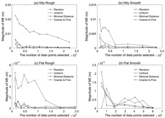
Figure 6.
The magnitude of mean error (ME) versus the number of data points of thinned point clouds for the four terrain surfaces: (a) hilly rough, (b) hilly smooth, (c) flat rough, and (d) flat smooth.
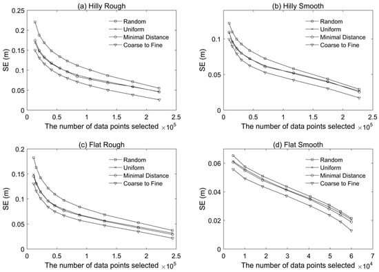
Figure 7.
The standard error (SE) versus the number of data points of thinned point clouds for the four terrain surfaces: (a) hilly rough, (b) hilly smooth, (c) flat rough, and (d) flat smooth.
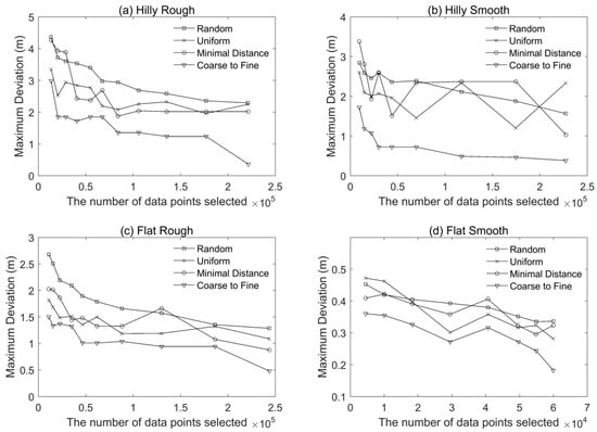
Figure 8.
The maximum deviation versus the number of data points of thinned point clouds for the four terrain surfaces: (a) hilly rough, (b) hilly smooth, (c) flat rough, and (d) flat smooth.
5. Discussion
The minimal distance method and the uniform method are algorithmically different, leading to different sub-sampled point clouds. However, these two methods tend to produce a sub-sample of largely homogenous distribution. This is likely the reason for similar RMSE values shown in Figure 4. Therefore, either method can be considered if one wishes to obtain an evenly distributed sub-sample.
The coarse-to-fine method is developed for sub-sampling point clouds that represent terrain surfaces. Although it was tested using airborne LiDAR-derived terrain point clouds, it is expected that it can readily be applied to terrain point clouds obtained using other surveying techniques. The coarse-to-fine method is able to produce a thinned point cloud that is adapted to local terrain surface roughness and can lead to more uniform local RMSE values over the whole area of interest.
For a given threshold RMSE in the coarse-to-fine method, the set of data points selected is affected by (1) the interval (e.g., 0.2 m used in Section 4.1) of the voxel edge length decreasing from a large value (i.e., coarse-resolution) to a small value (i.e., fine-resolution), and (2) the size of individual sub-areas. When a smaller interval is used, more varied data density bands are available. This will lead to a sub-sampled point cloud that has a smaller difference to the original point cloud, which is confirmed by the analysis results shown in Figure 9a. When a smaller sub-area size (i.e., more sub-areas) is used, the local surface roughness or complexity is better represented by the finer resolution, which also leads to a more favourable sub-sampled point cloud (Figure 9b). However, the increase in accuracy is less significant when the number of sub-areas used is large (e.g., from 400 to 900 sub-areas).
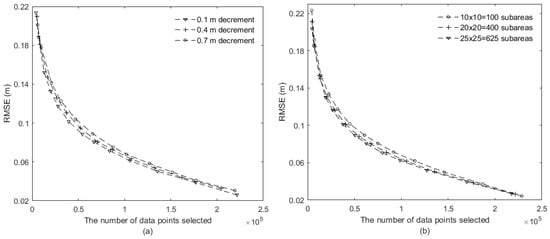
Figure 9.
The coarse-to-fine method for the hilly rough surface: (a) the effect of the decreasing interval of voxel edge length under the same number of 20 × 20 = 400 sub-areas, (b) the effect of the sub-area size under the same decreasing interval of 0.2.
The coarse-to-fine method is area (or block) based. Within a single local area, the relative importance of data points is not evaluated. The data density is adapted to only the between-block variation in surface roughness (often calculated over a particular scale), which can lead to an abrupt change in data density at the edges of the blocks. This issue may be mitigated by using a smaller block size and a smaller decrement internal for density reduction. In this study, the TIN with linear interpolation is used for prediction. However, the coarse-to-fine method can be readily implemented using other interpolation methods.
As shown in Figure 4, the spatial variation of data density of the thinned point cloud has a large correlation with that of the surface roughness map, and as such it may be used to infer the local roughness of the terrain surface.
A simple area partition method (i.e., square blocks) was used in this study. As a suggestion for further work, it would be interesting to investigate the performance of the coarse-to-fine method when more complex area partition methods (e.g., over-segmentation approaches such as voxel cloud connectivity segmentation and point cloud local variation [29,30,31,32,33]) were used. Such methods may take into account the terrain surface complexity for the area partition.
6. Conclusions
In this article, a simple non-stationary data sampling method for reducing point cloud density was investigated. The application of this method to the LiDAR datasets confirms its ability to produce a thinned point cloud with a data density (in sub-areas) which is adapted to local terrain surface roughness. For the different types of terrain surfaces, it was confirmed that the coarse-to-fine method performed more effectively than several other sub-sampling methods considered.
Author Contributions
L.F and P.M.A. have contributed to conceptualization, methodology and writing—review and editing. L.F. carried out the investigation and the formal analysis, in addition to writing—original draft preparation.
Funding
This research was funded by “Natural Science Foundation of Jiangsu Province, grant number BK20160393” and “the University internal support RDF, grant number RDF-15-01-52 & RDF-18-01-40”.
Acknowledgments
LiDAR data access is based on [LiDAR, ground] services provided by the OpenTopography Facility with support from the National Science Foundation under NSF Award Numbers 1226353 & 1225810. Lidar data acquisition completed by the National Center for Airborne Laser Mapping (NCALM - http://www.ncalm.org). NCALM funding provided by NSF’s Division of Earth Sciences, Instrumentation and Facilities Program. EAR-1043051. https://doi.org/10.5069/G9PR7SX0.
Conflicts of Interest
The authors declare no conflict of interest.
References
- Liu, X. Airborne LiDAR for DEM generation: Some critical issues. Prog. Phys. Geogr. 2008, 32, 31–49. [Google Scholar]
- Brasington, J.; Vericat, D.; Rychkov, I. Modeling river bed morphology, roughness, and surface sedimentology using high resolution terrestrial laser scanning. Water Resour. Res. 2012, 48, W11519. [Google Scholar] [CrossRef]
- Montreuil, A.L.; Bullard, J.E.; Chandler, J.H.; Millett, J. Decadal and seasonal development of embryo dunes on an accreting macrotidal beach: North Lincolnshire, UK. Earth Surf. Process. Landf. 2013, 38, 1851–1868. [Google Scholar] [CrossRef]
- Zhou, Q.M.; Chen, Y.M. Generalization of DEM for terrain analysis using a compound method. ISPRS J. Photogramm. Remote Sens. 2011, 66, 38–45. [Google Scholar] [CrossRef]
- Chen, C.F.; Yan, C.Q.; Cao, X.W.; Guo, J.Y.; Dai, H.L. A greedy-based multiquadric method for LiDAR-derived ground data reduction. ISPRS J. Photogramm. Remote Sens. 2015, 102, 110–121. [Google Scholar] [CrossRef]
- Anderson, E.S.; Thompson, J.A.; Austin, R.E. LIDAR density and linear interpolator effects on elevation estimates. Int. J. Rem. Sens. 2005, 26, 3889–3900. [Google Scholar] [CrossRef]
- Liu, X.; Zhang, Z. Effects of LiDAR data reduction and breaklines on the accuracy of digital elevation model. Surv. Rev. 2011, 43, 614–628. [Google Scholar] [CrossRef]
- Yilmaz, M.; Uysal, M. Comparison of data reduction algorithms for LiDAR-derived digital terrain model generalization. Area 2016, 48, 521–532. [Google Scholar] [CrossRef]
- Li, Z.L. Theoretical models of the accuracy of digital terrain models: An evaluation and some observations. Photogramm. Rec. 1993, 14, 651–660. [Google Scholar] [CrossRef]
- Hu, P.; Liu, X.H.; Hu, H. Accuracy assessment of digital elevation models based on approximation theory. Photogramm. Eng. Remote Sens. 2009, 75, 49–56. [Google Scholar] [CrossRef]
- Kraus, K.; Karel, W.; Briese, C.; Mandlburger, G. Local accuracy measures for digital terrain models. Photogramm. Rec. 2006, 21, 342–354. [Google Scholar] [CrossRef]
- Aguilar, F.J.; Agüera, F.; Aguilar, M.A.; Carvajal, F. Effects of terrain morphology, sampling density, and interpolation methods on grid DEM accuracy. Photogramm. Eng. Remote Sens. 2005, 71, 805–816. [Google Scholar] [CrossRef]
- Aguilar, F.J.; Aguilar, M.A.; Agüera, F.; Sánchez, J. The accuracy of grid digital elevation models linearly constructed from scattered sample data. Int. J. Geogr. Inform. Sci. 2006, 20, 169–192. [Google Scholar] [CrossRef]
- Guo, Q.; Li, W.; Yu, H.; Alvarez, O. Effects of topographic variability and lidar sampling density on several DEM interpolation methods. Photogramm. Eng. Remote Sens. 2010, 76, 1–12. [Google Scholar] [CrossRef]
- Fan, L.; Atkinson, P.M. Accuracy of digital elevation models derived from terrestrial laser scanning data. IEEE Geosci. Remote Sens. Lett. 2015, 12, 1923–1927. [Google Scholar] [CrossRef]
- Heckbert, P.S.; Garland, M. Survey of Polygonal Surface Simplification Algorithms; Technical Report; School of Computer Science, Carnegie Mellon University: Pittsburgh, PA, USA, 1997. [Google Scholar]
- Floriani, L.D.; Falcidieno, B.; Nagy, G.; Pienovi, C. A hierarchical structure for surface approximation. Comput. Graph. 1984, 8, 183–193. [Google Scholar] [CrossRef]
- Lee, J. Comparison of existing methods for building triangular irregular network models of terrain from grid digital elevation models. Int. J. Geogr. Inf. Sci. 1991, 5, 267–285. [Google Scholar] [CrossRef]
- Heller, M. Triangulation algorithms for adaptive terrain modelling. In Proceedings of the 4th International Symposium on Spatial Data Handling, Zürich, Switzerland, 23–27 July 1990; pp. 163–174. [Google Scholar]
- Chang, K. Introduction to Geographic Information Systems, 4th ed.; McGraw-Hill: New York, NY, USA, 2007. [Google Scholar]
- Hughes, M.; Lastra, A.A.; Saxe, E. Simplification of global-illumination meshes. Comput. Graph. Forum 1996, 15, 339–345. [Google Scholar] [CrossRef]
- Oryspayev, D.; Sugumaran, R.; DeGroote, J.; Gray, P. LiDAR data reduction using vertex decimation and processing with GPGPU and multicore CPU technology. Comput. Geosci. 2012, 43, 118–125. [Google Scholar] [CrossRef]
- Atkinson, P.M.; Curran, P.J.; Webster, R. Sampling remotely sensed imagery for storage, retrieval and reconstruction. Prof. Geogr. 1990, 42, 345–353. [Google Scholar] [CrossRef]
- Atkinson, P.M.; Lloyd, C.D. Non-stationary variogram models for geostatistical sampling optimisation: An empirical investigation using elevation data. Comput. Geosci. 2007, 33, 1285–1300. [Google Scholar] [CrossRef]
- Lloyd, C.D.; Atkinson, P.M. Non-stationary approaches for mapping terrain and assessing uncertainty. Trans. Geograph. Inform. Syst. 2002, 6, 17–30. [Google Scholar] [CrossRef]
- Dovrat, O.; Lang, I.; Avidan, S. Learning to Sample. Available online: https://arxiv.org/abs/1812.01659 (accessed on 12 April 2019).
- Brubaker, K.M.; Myers, W.L.; Drohan, P.J.; Miller, D.A.; Boyer, E.W. The use of LiDAR terrain data in characterizing surface roughness and microtopography. Appl. Environ. Soil Sci. 2013, 2013, 891534. [Google Scholar] [CrossRef]
- Fan, L.; Atkinson, P.M. A new multi-resolution based method for estimating local surface roughness from point clouds. ISPRS J. Photogramm. Remote Sens. 2018, 144, 369–378. [Google Scholar] [CrossRef]
- Papon, J.; Abramov, A.; Schoeler, M.; Worgotter, F. Voxel cloud connectivity segmentation—supervoxels for point clouds. In Proceedings of the IEEE Conference on Computer Vision and Pattern Recognition (CVPR), Portland, OR, USA, 23–28 June 2013; pp. 2027–2034. [Google Scholar]
- Ben-Shabat, Y.; Avraham, T.; Lindenbaum, M.; Fischer, A. Graph based over-segmentation methods for 3D point clouds. Comput. Vis. Image Underst. 2018, 174, 12–23. [Google Scholar] [CrossRef]
- Zhu, Q.; Li, Y.; Hu, H.; Wu, B. Robust point cloud classification based on multi-level semantic relationships for urban scenes. ISPRS J. Photogramm. Remote Sens. 2017, 129, 86–102. [Google Scholar] [CrossRef]
- Wang, Y.; Cheng, L.; Chen, Y.; Wu, Y.; Li, M. Building point detection from vehicle-borne LiDAR data based on voxel group and horizontal hollow analysis. Remote Sens. 2016, 8, 419. [Google Scholar] [CrossRef]
- Poux, F.; Neuville, R.; Van Wersch, L.; Nys, G.A.; Billen, R. 3D point clouds in archaeology: Advances in acquisition, processing and knowledge integration applied to quasi-planar objects. Geosciences 2017, 7, 96. [Google Scholar] [CrossRef]
© 2019 by the authors. Licensee MDPI, Basel, Switzerland. This article is an open access article distributed under the terms and conditions of the Creative Commons Attribution (CC BY) license (http://creativecommons.org/licenses/by/4.0/).