Accurate Measurement of Tropical Forest Canopy Heights and Aboveground Carbon Using Structure From Motion

Abstract

Unmanned aerial vehicles are increasingly used to monitor forests. Three-dimensional models of tropical rainforest canopies can be constructed from overlapping photos using Structure from Motion (SfM), but it is often impossible to map the ground elevation directly from such data because canopy gaps are rare in rainforests. Without knowledge of the terrain elevation, it is, thus, difficult to accurately measure the canopy height or forest properties, including the recovery stage and aboveground carbon density. Working in an Indonesian ecosystem restoration landscape, we assessed how well SfM derived the estimates of the canopy height and aboveground carbon density compared with those from an airborne laser scanning (also known as LiDAR) benchmark. SfM systematically underestimated the canopy height with a mean bias of approximately 5 m. The linear models suggested that the bias increased quadratically with the top-of-canopy height for short, even-aged, stands but linearly for tall, structurally complex canopies (>10 m). The predictions based on the simple linear model were closely correlated to the field-measured heights when the approach was applied to an independent survey in a different location ($R^2$ = 67% and RMSE = 1.85 m), but a negative bias of 0.89 m remained, suggesting the need to refine the model parameters with additional training data. Models that included the metrics of canopy complexity were less biased but with a reduced $R^2$. The inclusion of ground control points (GCPs) was found to be important in accurately registering SfM measurements in space, which is essential if the survey requirement is to produce small-scale restoration interventions or to track changes through time. However, at the scale of several hectares, the top-of-canopy height and above-ground carbon density estimates from SfM and LiDAR were very similar even without GCPs. The ability to produce accurate top-of-canopy height and carbon stock measurements from SfM is game changing for forest managers and restoration practitioners, providing the means to make rapid, low-cost surveys over hundreds of hectares without the need for LiDAR.

1. Introduction

The effective management of tropical forests is often dependent on high-quality information about the spatial distribution and condition of forest types [1,2,3]. Spatial measurements of forest quality are, therefore, important for prioritizing a range of conservation interventions and are especially critical in planning restoration work [4]. Globally, there are approximately 1 billion hectares of degraded tropical forests that have the potential to be restored [5], but active interventions are expensive and the cost–benefit ratios for different interventions vary with forest condition [6]. In particular, unmanaged young forests have been shown to sequester carbon rapidly [7], but the diversity and capital value of these forests (i.e., for timber or non-timber forest products) is likely to be enhanced through active management [8,9,10]. Furthermore, the biomass and species composition of secondary forests can vary considerably over small spatial scales, and conditions can change rapidly during natural regeneration. Therefore, the planning of appropriate restoration interventions requires the timely delivery of fine-resolution forest condition data [4].

Airborne laser scanning (ALS, which is also commonly referred to as LiDAR) provides highly detailed structural information that is widely used in forestry and for assessing forest carbon dynamics [11,12]. Discrete-return LiDAR devices work by actively emitting laser pulses that detect canopy surfaces from the uppermost leaves through to the ground, resulting in a cloud of points (point clouds) that describe the three-dimensional structure of the forests. By building up a ground surface or Digital Terrain Model (DTM) from ground returns, canopy heights can then be calculated through a normalisation of the point cloud (i.e., a subtraction of the terrain from the surface; [13]). Ground returns are far less frequent than those from the upper canopy but are, nevertheless, frequent enough to measure the canopy height with an accuracy of less than 1 m [2]. Such measurements have produced accurate maps of the carbon density [12,14], stand structure, and understory condition [15,16] in tropical forests. However, LiDAR is rarely available to forest restoration practitioners in the tropics because of the high cost of deploying manned aircraft. Now three-dimensional (3-D) mapping with unmanned aerial vehicles (UAVs) holds the promise of providing a cheaper and more accessible alternative requiring minimal training.

Aerial photography from UAVs is being applied in many industries and increasingly in conservation management, including the mapping of forest structure in restoration projects [17,18,19,20]. However, techniques for constructing 3-D forest canopy maps from UAV images lag behind recent advances in data capture. Digital surface models of similar quality to those produced by LiDAR can be constructed from high-resolution photographs taken from UAVs, using a technique known as Structure from Motion (SfM) [21]. The three-dimensional structure of the canopy surface is retrieved from two-dimensional images because the position of features shared between multiple overlapping images (of which the locations are known from GPS tags and further resolved during the reconstruction process) can be estimated in 3-D space, using a process analogous to triangulation. However, by contrast to LiDAR, structure from motion can have a poor penetrability to the ground level because canopy openings are too small (a) to allow an equivalent illumination of the ground and canopy, which results in an underexposure in imagery, and (b) to be viewed from the oblique angles required for positional triangulation [22,23]. Therefore, ground positions are only identified where gaps of sufficient sizes extend to the forest floor, and these can be very rare or absent in dense tropical forests. Ground classification algorithms that follow a process of dividing point clouds into grid cells, identifying the lowest points, and adding adjacent points according to simple rules [24] will always have a positive bias in their estimation of ground position (Figure 1). The positive bias in the DTMs produced by SfM, which results in a negative bias in estimated canopy heights, has raised concerns about the validity of the technique for measuring forest properties [25,26,27].

Despite the paucity of ground points captured using SfM, it may be possible to correct the ground position estimates if biases are consistent and predictable. By developing models that use properties from the digital surface model to predict an overestimation of the DTM/an underestimation of the canopy height, a correction may be applied to remove the bias. Some studies assessing the correspondence of SfM and LiDAR canopy height measurements have done so using root mean squared error (RMSE) only [25,28], which measures the average differences of predictions from the truth. Yet, if SfM consistently underestimates canopy heights, these measurements will contain both systematic and random error components, which should be accounted for separately [26]. Measuring systematic error is straightforward if a dataset without error is available. This can, then, be used to produce a correction function capable of generalising to new data outside of the training set. This approach has been used in numerous fields, including field measurements of trees [29]. A recent study [30] was able to predict the aboveground biomass from numerous structural and spectral metrics extracted from SfM point clouds using machine learning. However, including numerous metrics is known to produce overfitted models that fail to generalise to unseen data and novel situations; this is known as the bias-variance trade-off [31]. Therefore, when including a correction for SfM-based canopy height assessments, it is preferable to build simple but robust models with metrics that are likely to be consistent across sites and to demonstrate a high-performance when applied to independent data.

This study, focusing on a regenerating tropical rain forest in an ecosystem restoration concession in Indonesia, compares the stand level top-of-canopy height and aboveground carbon density estimates produced by SfM and airborne LiDAR. We calculate the bias in the SfM measurements and use this to produce a robust correction, assuming that LiDAR provides an unbiased benchmark against which to compare other approaches. Finally, we trial the ability to apply a correction at an independent location using a different UAV where LiDAR data were also present. To the best of our knowledge, this is the first attempt to produce and validate such a correction on independent data. From these corrected canopy heights, the aboveground biomass can be calculated, which is highly correlated with important measures of forest quality, including aboveground carbon stocks [12,32], rates of carbon sequestration [7], and biodiversity [33,34]. This approach has the potential to greatly increase the utility of UAV surveys for tracking changes in forest quality and direct restoration without the need for wall-to-wall LiDAR coverage.

2. Materials and Methods

2.1. Study Site

The work was conducted at Hutan Harapan (trans. Hope Rainforest) on the island of Sumatra, the first of several Ecosystem Restoration Concessions established in Indonesia. These concessions are an Indonesian government initiative to lease tracts of heavily degraded forest to private organisations for long-term restoration. Hutan Harapan is a 98,455 hectare fragment of the lowland forests that dominated the island prior to the 20th-century agricultural expansion. Long-term experiments at Hutan Harapan are exploring the effects of various management interventions on reforestation, biodiversity conservation, capacity for carbon capture, and economic potential [10,35]. Two sites were surveyed: (1) an 82-ha area, close to the Kapas river composed of an even-aged regenerating stand averaging 9 m in height (s.d. = 5 m) and with the remainder less even-aged and averaging 15 m in height (s.d. = 8 m) with many trees taller than 30 m, and (2) a 48-ha area close to the concession’s central nursery, known as Bato, averaging 17 m in height (s.d. = 8 m). The intersecting LiDAR and SfM canopy height models are shown in Figure 2.

2.2. Photographic and LiDAR surveys

The LiDAR data were collected on 24 October 2014. A Leica ALS70 plus LiDAR device was mounted within a Pilatus Porter PC6 aircraft and flown at an altitude of 800 m and ground speed of 100 km per hour. The ground points were classified within the LiDAR point cloud using the default parameters of the LAStools [36] (version 1.2) algorithm lasground, set to “Wilderness” which specifies a grid size for the initial low-point detection of 5 m and then converted to a 0.33 m resolution DTM raster using las2dem. A pitfree canopy height model raster was also produced using LAStools following the method of Reference [37]. At present, this is the most precise method for measuring canopy heights across landscapes and is, thus, an appropriate benchmark against which to judge the success of our UAV-based SfM measurements.

The two sites were mapped separately with two different UAVs. The Kapas site was surveyed on 21 March 2016 using a Tarot Ironman 650 multirotor UAV with a Pixhawk Flight controller and Canon S110 camera using a Canon Hackers Development Kit (CHDK) intervalometer. The UAV was flown at 140 m above ground level (relative to the launch site) with images collected every three seconds. The images were geotagged post hoc through a fusion with flight logs using ExifTool through the GeoSetter graphical user interface (https://www.geosetter.de/en/main-en/); correct time-stamp alignment was achieved by ensuring the position of transect turns that correspond with rotations in the camera imagery. The Bato site was flown on 16 April 2017 using a 3DR Solo multirotor UAV with a Parrot Sequoia camera. The UAV was flown at 120 m above ground level with the images collected every three seconds. Surveys at each location involved four flights and were completed in less than two hours in total. The images were georeferenced in real-time using GPS information from the Sequoia’s on-board GPS. In both cases, SfM was implemented in Agisoft Photoscan (version 1.2.4) to produce point clouds from which DTMs were generated using the Photoscan algorithm for ground classification, setting the initial grid size to 50 m to ensure the detection of low points and setting the angle and distance parameters to zero. Smaller grid sizes contained large variations in low-point detection, whereas large grid sizes were considered inappropriate for capturing topography. After excluding anomalous low points (i.e., points erroneously located outside the normal point distribution) which were detected automatically during ground classification in Photoscan, digital surface and terrain model rasters were generated from classified point clouds at a 0.33 m resolution, and canopy height models were produced as the difference between these. The data from the Kapas site was used exclusively for modeling the correction, while the data from the Bato site was used for independent validation.

2.3. Calculating the Correction

The SfM surface model rasters were georeferenced to the LiDAR by manually identifying ground control points in the LiDAR digital surface model and applying a linear transformation with a nearest neighbour resampling using the georeferencer plugin in QGIS (version 2.18). The SfM and LiDAR surface models were cropped to their intersections (80 ha at Kapas and 48 ha at Bato). The canopy height models were aggregated to the mean and standard deviations in the top-canopy height at a 0.25 ha (50 × 50 m) scale, and any areas with less than a 75% coverage were excluded. This yielded 298 observations at Kapas and 148 observations at Bato. The standard deviation maps were used as an additional predictor describing the variation in canopy height (V). Digital surface models were also aggregated to a 0.25 ha scale and used to calculate the topographic position index (TPI) at a 2.25 ha scale (150 × 150 m). The TPI was calculated for each pixel as $TPI=x-\frac{1}{n}{\displaystyle \sum _{i=1}^n}{X}_i$, where x is the elevation of the focal pixel and X is the vector of elevation values that includes x and all of the immediately adjacent pixels ($n=9$). In this sense, TPI provides a measure of the vertical position of the canopy relative to the position of the surrounding canopy (T) and is, thus, referred to from here as the canopy position index; it will be positive on hill tops and when the forest is tall relative to its surroundings and will be negative for valley bottoms and when the forest is short relative to its surroundings.

Two initial linear models were fitted to predict the LiDAR top-of-canopy height from the SfM top-of-canopy height. These models attempted to explain the basic function of the relationship, which was clearly nonlinear, without including additional variables. The models were as follows:

$$y_i={\beta }_0+{\beta }_1{x}_i+{ϵ}_i$$

(1)

$$y_i^2={\beta }_0+{\beta }_1{x}_i+{ϵ}_i$$

(2)

where y and x are the LiDAR and SfM measured top-of-canopy heights respectively, for each of the i 0.25-ha locations. In Equation (2), y was squared prior to model fitting in order to address the nonlinearity. More complex models were also developed to assess the additional predictive value of including the interactions between the SfM-measured top-of-canopy height, the canopy position index T, and the canopy height variation V, as follows:

$$y_i={\beta }_0+{\beta }_1{T}_i+{\beta }_2{x}_i+{ϵ}_i$$

(3)

$$y_i={\beta }_0+{\beta }_1{V}_i+{\beta }_2{x}_i+{ϵ}_i$$

(4)

$$y_i^2={\beta }_0+{\beta }_1{T}_i+{\beta }_2{x}_i+{ϵ}_i$$

(5)

$$y_i^2={\beta }_0+{\beta }_1{V}_i+{\beta }_2{x}_i+{ϵ}_i$$

(6)

For each model, the residual error $ϵ$ was estimated as a normal distribution with a mean of zero and a standard error of $\sigma$. A fivefold cross validation was implemented in the R package Caret (version 6.0-78) to assess the predictive performance as the average out-of-set root mean squared error (RMSE) and $R^2$ of the prediction across the five folds. Predictions were then made for Bato and compared against the LiDAR measurements. In order to assess the effect of georeferencing SfM surface models, we carried out the same comparisons with the LiDAR models both prior to and after georeferencing. As part of this comparison, we converted the top-of-canopy height measurements (H) to the aboveground carbon density ($ACD$) using the following equation developed by Jucker et al. (2017) [14] for Southeast Asian rain forests:

$$ACD=0.567H^{0.554}{A}^{1.081}{\rho }^{0.186}$$

(7)

where $\rho$ is the wood density, calculated as $\rho =0.385H^{0.097}$, and A is the basal area, calculated as $A=1.12H$. This enabled us to assess how the error in top-of-canopy heights is inflated when converting to biomass. We assessed the performance of the corrections as the $R^2$ of prediction, RMSE, and bias when comparing observations at the 0.25-ha scale. A linear regression also was used to test whether a relationship between the bias and topographic position remained in the validation site (Bato) after correction.

3. Results

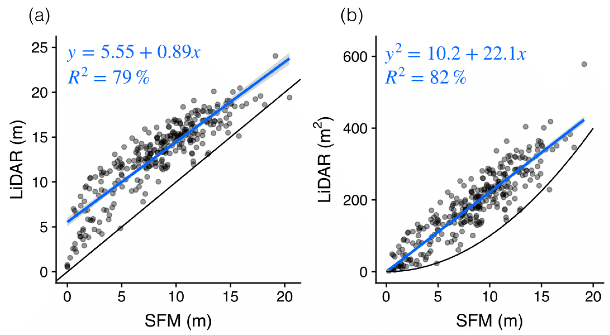
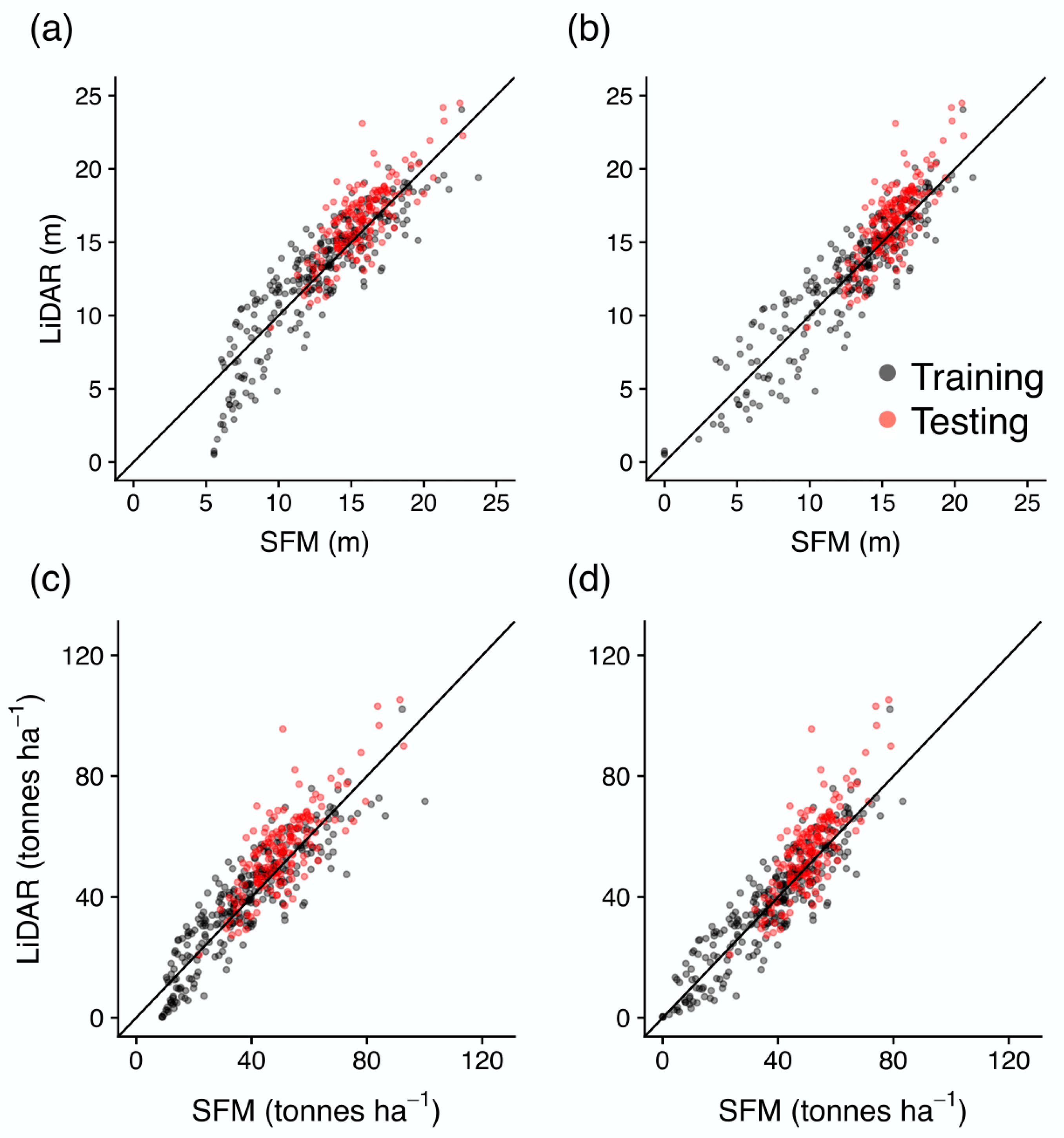
Developing the Tree Height Correction Model

The top-of-canopy height measured by SfM was strongly correlated with the LiDAR-measured top-of-canopy height (Pearson’s $r=0.89$) but the SfM measurements contained a substantial error with an RMSE of 5.08 m, $39\%$ of the mean LiDAR-measured top-of-canopy height (Figure 3). However, a negative bias of 4.66 m, similar in magnitude to the mean error, made it possible to produce straightforward but powerful empirical corrections (Figure 3).

Both of the models used to fit the relationship between the SfM- and LiDAR-measured heights explained a large proportion of the variation ($R_{model1}^2=79\%$ and $R_{model2}^2=82\%$), and the resulting predictions had a substantially lower RMSE relative to the uncorrected SfM measurements. Model 1 fit the data well on average but overestimated the top-of-canopy height for the shortest canopies (Figure 3). The linear model fit to the squared SfM measurements (Model 2) increased the $R^2$ of the prediction by removing the nonlinearity from the relationship, which reduced the bias in the estimates for the shortest canopies, but the correction became progressively smaller in magnitude with the top-of-canopy height (as seen by the model fit approaching the 1:1 line). This suggests that the top-of-canopy height will be poorly corrected for the tallest canopies, which is problematic because these contain a disproportionate amount of the aboveground carbon (Figure 3). Because both models performed well and had desirable properties at different ends of the canopy height range, they were both used for further model development. The inclusion of the interaction between the top-of-canopy height and the canopy position index led to small increases in the $R^2$ of the prediction to 83.0% and 83.2% respectively for Models 1 and 2. Similarly, the inclusion of the interaction between the top-of-canopy height and the top-of-canopy height variation yielded increases in the $R^2$ of the prediction to 82.0% and 82.8% respectively for Models 1 and 2.

In out-of-set testing, Model 1 and Model 2 performed similarly in terms of predictive performance (

Table 1. The out-of-set model validation for top-of-canopy heights and aboveground carbon density (AGCD). The correction models were developed at a site 5 km away from the site used for testing, using a different model of UAV with a different camera and surveyed one year earlier. Named models and fitted functions are presented along with the performance metrics calculated by comparison to the LIDAR gold-standard at 0.25-ha scale. The total estimates of the aboveground biomass for the entire study area are also shown. Comparisons are made for the models with and without georeferencing (no GCPs).

Canopy Height Model	Canopy Height (m)
	Mean	s.d.	${\mathit{R}}^{\mathbf{2}}$	RMSE	Bias
LiDAR	16.6	2.83	-	-	-
SfM	11.4	2.63	0.67	5.45	−5.20
Model 1 $y=5.55+0.89x$	15.7	2.34	0.67	1.85	−0.89
Model 2 $y^2=10.2+21.1x$	15.8	1.80	0.66	1.90	−0.84
Model 3 $y=5.49+0.25T+0.93x-0.04xT$	15.9	1.93	0.65	1.85	−0.69
Model 4 $y=2.91+0.80V+1.03x-0.054xV$	15.7	1.81	0.64	1.96	−0.90
Model 5 $y^2=1.59+0.06T+22.5x-0.36xT$	15.9	1.53	0.68	1.91	−0.69
Model 6 $y^2=15.1+2.56V+15.1x+0.61xV$	15.8	1.96	0.67	1.84	−0.81
Model 1 no GCPs	15.6	2.43	0.51	2.25	−1.02
Model 2 no GCPs	15.7	1.88	0.51	2.20	−0.95
Canopy Height Model	Above-Ground Carbon Density (Tonnes${\mathit{ha}}^{-\mathbf{1}}$)					Total AGCD (tonnes)
	Mean	s.d.	${\mathit{R}}^{\mathbf{2}}$	RMSE	Bias
LiDAR	56.3	16.1	-	-	-	8332
SfM	30.7	12.0	0.68	27.2	−25.6	4537
Model 1 $y=5.55+0.89x$	51.2	12.9	0.68	10.4	−5.07	7582
Model 2 $y=2.91+0.80V+1.03x-0.054xV$	51.3	9.7	0.67	11.1	−5.04	7586
Model 3 $y=5.49+0.25T+0.93x-0.04xT$	52.1	10.4	0.64	10.8	−4.22	7707
Model 4 $y=2.91+0.80V+1.03x-0.054xV$	50.9	9.6	0.64	11.5	−5.35	7504
Model 5 $y^2=1.59+0.06T+22.5x-0.36xT$	52.0	8.2	0.68	11.2	−4.34	7690
Model 6 $y^2=15.1+2.56V+15.1x+0.61xV$	51.5	10.7	0.68	10.5	−4.83	7717
Model 1 no GCPs	50.6	13.4	0.53	12.5	−5.71	7487
Model 2 no GCPs	50.7	10.1	0.52	12.5	−5.60	7502

). Both models produced vastly improved top-of-canopy height estimates compared with the uncorrected SfM measurements, reducing the mean error from 5.45 m to less than 1.90 m (Table 1). The close correspondence between the corrected SfM and LiDAR measurements can be seen in Figure 4a,b. However, a mean bias of −0.89 m and −0.84 m remained after a correction for Models 1 and 2 respectively. The bias for the tallest quartile of the sampled stands was −1.88 m for Model 1 and −2.54 for Model 2 (Figure 4). The addition of the canopy position index and the canopy height variation as predictors in an interaction with the SfM-measured top-of-canopy height did improve the predictive performance in out-of-set testing, although this was fairly minimal with these models failing to reduce the average error or bias for the tallest quartile when compared with Model 1. Model 1 (linear model estimate = 0.19, t${}_{146}$ = 5.76, p < 0.0001) and Model 2 (linear model estimate = 0.15, t${}_{146}$ = 4.11, p < 0.0001) both retained significant effects of the topographic position index on bias, while the inclusion of the canopy position index in Models 3 and 5 removed these relationships. These models also reduced the average bias by 0.20 m and 0.15 m compared with Models 1 and 2, respectively (Table 1), but they had a much greater negative bias for the tallest quartile of −2.63 and −2.58 for Models 3 and 5 respectively.

The estimates were more accurate compared to the uncorrected SfM measurements after a nonlinear conversion to aboveground carbon densities. The 31% bias in the uncorrected top-of-canopy heights was converted into a 45% bias in aboveground carbon density. However, the bias in the corrected aboveground carbon densities was reduced to only 9% in Model 1 and 7% in Model 3. Despite an exacerbation of the negative bias for the tallest canopies in Model 2, this was offset by more accurate predictions for intermediate height canopies (Figure 4) so that the total biomass estimation remained similar to that generated by Model 1 (Table 1). The improved predictive performance achieved by adding a canopy position index and canopy height variation as predictors in the interaction with the SfM-measured top-of-canopy height was translated into a further improvement in the aboveground carbon density estimation. Thus, although the error was not reduced by the more complex models, the bias was, which produced average and total aboveground carbon density estimates closer to those measured by the LiDAR (Table 1).

A failure to georeference the SfM models led to a reduced correspondence with the LiDAR measurements, revealing the lower spatial accuracy of structure from motion without ground control points relative to LiDAR (Table 1). Despite this, the corrected average and total aboveground carbon density measurements remained very similar, both with and without georeferencing (Table 1).

4. Discussion

Our study demonstrates the high precision of 3-D information created by Structure from Motion (SfM) using photographs taken with Unmanned Aerial Vehicles (UAVs). The stand-level structural attributes, including top-of-canopy height and aboveground carbon density, were accurately measured from these models once the systematic bias, arising from a lack of ground observations, was accounted for. The uncorrected SfM top-of-canopy heights were substantially underestimated, assuming LIDAR gives reliable measurements, as has been shown previously [27,28,30,38]. SfM is undoubtedly poor at detecting ground points in a closed canopy forest [22,28], but its effectiveness at reconstructing 3-D surfaces [26,39], coupled with the predictable manner in which top-of-canopy height is underestimated, make this problem straightforward to address. While previous assessments of forest heights have suggested that SfM is prone to excessive error [25,40], we have shown that this is primarily comprised of bias that can be almost completely removed by our corrections [41]. LiDAR-measured top-of-canopy heights were predicted from SfM with error rates of only 7%, as validated on an independent data set. This has an enormous potential for enabling forest managers and restoration practitioners, who do not have access to full coverage LiDAR surveys, to make accurate measurements of forest resources [4].

4.1. Improved Accuracy of SfM Measurements

The top-of-canopy heights were underestimated by SfM but the bias was consistent enough to enable a correction [41]. Two linear models were produced that generated excellent fits to the training data but suggested different bias patterns. The model that predicted untransformed LiDAR top-of-canopy heights (model 1) indicated that bias was at a maximum of 5.55 m for the shortest stands and decreased by 0.11 m for each additional metre of height (Figure 3a); consequently, the average bias was 3.35 m for 20-m tall stands. The model that predicted squared LiDAR top-of-canopy heights (Model 2) indicated a nonlinear bias, with a minimum close to zero at the ground (i.e., when vegetation was absent) which increased to a maximum of 5.57 m for 10-m tall stands and decreased thereafter (Figure 3b). Although Model 2 produced a slightly better fit to the data ($R^2$ increased from 79% to 82%), the linear nature of Model 1 makes it more robust in taller stands, whereas Model 2 will always overestimate the top-of-canopy heights for stands taller than 21.5 m (as can be seen by the intersection of the 1:1 line in Figure 3b). This is important because Southeast Asian forests are known to have top-of-canopy heights up to 50 m [14] that would be substantially overestimated (average error resulting from the correction would be 236%). Including taller stands during model development should ameliorate this issue but at the expense of accuracy for the shortest stands. Alternatively nonlinear models that better describe the bias relationship with the top-of-canopy height may provide the best of both models. Nevertheless, Model 2 makes good sense mechanistically: After clearance, lowland tropical forests exhibit a pulse of rapid growth that produces homogeneous dense swathes of vegetation; the structural complexity then increases through a combination of differential growth and mortality-induced gap formation (e.g., References [28,42] and references therein). The occlusion of ground and lower canopy observations increases as the bare ground transitions to early successional vegetation but then decreases as stands transition towards structural complexity. This occurred once the top-of-canopy height exceeded 10 m at our site in Indonesia. This finding confirms that SfM top-of-canopy height bias is greatest in the shortest stands, but when both DTM and canopy errors are combined, rather than canopy errors alone, the bias is negative rather than positive as found by Roşca et al. (2018) [43].

The corrections we developed produced excellent estimates of the top-of-canopy height and biomass at an independent location not included during the model development. This demonstrates the generality of our approach even to sites where LiDAR data are not available. Despite using a different UAV, with a different camera and flight parameters, the top-of-canopy height was estimated with the $R^2$ of prediction values of 67% and 66% for Models 1 and 2, respectively, and RMSEs of 1.85 m and 1.90 m (Table 1), respectively. The negative bias (approximately 0.9 m) that remained suggests that our correction may not be stable across sites and could be improved by using training data drawn from a greater diversity of sites, which remains a major limitation of most studies that predict canopy properties from SfM data (e.g., References [30,41,44,45,46]). The quadratic relationship may be less stable than the linear relationship across sites. Despite the prediction that Model 2 would produce overestimates for the tallest canopies, the reverse was observed, with a gross underestimation amplified during nonlinear conversion to aboveground carbon density (Figure 4b). This suggests that Model 1 generalised better to new areas and was more robust to conversion to aboveground carbon density. More complex Models (3–6) including interactions with the canopy position index and canopy height variation, suggested fairly subtle improvements that did not, in any case, improve both the mean error and bias compared with the simple models. However, Models 3 and 5, which included the canopy position index removed residual biases related to the topographic position which were not removed by Models 1 and 2. This suggests that topographic position is important in determining SfM bias, with a greater negative bias in valleys and less bias on ridge tops, which may be caused by DTM truncation due to the large size of the grid used during the development of the triangular irregular network (50 m). A similar study comparing LiDAR and SfM canopy height models in Cambodian forests found that SfM DTMs were of insufficient accuracy, but this may have in part been caused by the small grid size used (10 m), leading to a failure to reliably detect low points [40]. This highlights a trade-off between low-point detection and topographic truncation that requires further investigation. An alternative explanation is that ground occlusion is more pronounced in valley bottoms than on hill tops due to a combination of canopy and topographic features and is further exacerbated where the point density is low [47]. LiDAR surveys are also affected by these errors [26,48] but can be corrected using probabilistic models that account for differences in the ground detection, which is specific to the sensor [47]. As far as we are aware, no such models have yet been developed for SfM. However, an estimation of stand properties from SfM were improved in sugarcane when UAV survey transects were undertaken in both the North-South and East-West directions, probably as a result of improved ground detection from multiple viewing angles [49].

Recent studies have demonstrated that machine learning approaches can predict tree and stand level properties, including the aboveground biomass and leaf area index, from a diverse set of summary statistics derived from spectral and structural measurements obtained through SfM (e.g., Reference [30,44,45,46]). Yet, while these approaches are clearly effective at predicting held out observations, which are effectively subsets of the training data, they probably require considerable development to generalise well to new conditions and survey equipment. Our approach is far simpler, relying solely on the assumption that a canopy height underestimation at the stand-level changes predictably with the top-of-canopy height. This has been demonstrated for point measurements of sward height in grassland [50] and stand height in Maize [30]. However, our approach generated more accurate predictions across the gradient of stand heights, which was likely achieved by correcting a stand level (0.25 ha) property (i.e., top-of-canopy height) rather than point measurements [50]. It may be desirable to measure the top-of-canopy height at smaller scales, but it is likely that a variation in point cloud density, vegetation density, and topographic features will be greater at smaller scales, causing the relationship to break down [27].

4.2. Application in Other Forest Types

Our approach should generalise well across fairly similar conditions, but the canopy height bias relationship will probably need to be calibrated for specific forest types. This relationship is likely to depend on the configuration of gaps and canopy density which affect the depth and frequency at which the ground approximations are made [22]. SfM has been shown to accurately measure the top-of-canopy height of young plantations [23], open dry forest [26], open woodland [41], and forest fragments [28], where ground observations are abundant. The challenge is much greater in closed canopy forests, such as primary lowland tropical forests [43], which exhibit top-of-canopy heights in excess of 50 m [14] and have leaf area indices in excess of 6 m${}^2$ m${}^{-2}$ [51], where observations of the lower canopy may be extremely scarce. Our predictions may have been aided by the structural information provided by remnant trees, taller than 30 m, emerging from a canopy averaging 15m in height. In contrast, the greatest errors occurred in dense stands approximately 10 m in height. It is likely that the lack of structural complexity prevented the detection of low points, closer to the ground. In these situations, a machine learning approach that combines structural and spectral features to predict canopy height may prove more effective [30,44,45].

4.3. The Value of Ground Control Points

Failing to include ground control points (GCPs) reduced the correspondence between the LiDAR and the SfM estimates at the 0.25-ha scale, but the average and total above-ground carbon densities were robust even without GCPs. Accurate ground control points are essential for georeferencing SfM point clouds. They ensure that 3-D surfaces are correctly registered in space, and without them, vertical errors have been shown to increase according to a quadratic function with distance to the nearest GCP [52]. However, they can be hard to deploy in tropical forests where access is challenging and closed canopies limit their observation, and although GPS positions with differential correction can be accurate to 0.1 m, the error from typical handheld devices may exceed 10 m [28,53]. Our results indicate that GCPs are unnecessary if the main goal is to measure aboveground carbon densities at the scale of several hectares. However, if the goal is to track changes throughout time or to make measurements at smaller scales, e.g., to identify where active restoration activities need to take place [4], then a greater effort to accurately georeference SfM models is needed. One exciting option is to correct UAV-acquired geolocations using differential carrier-phase positioning to a precision of 2–3 mm. This approach has been shown to be highly effective for developing accurate models of ice flows using SfM, where the deployment of GCPs is impossible [54]. These systems are fairly expensive at present, and the coverage of the global navigation satellite system (GNSS), necessary to obtain this precision, is predominantly limited to the northern hemisphere, but an expansion to the equatorial and southern regions is expected in future.

5. Conclusions

Efforts to assess the extent to which LiDAR canopy height measurements can be replicated using stereo photogrammetry are now close to twenty years old [55]. Here, we have shown that they can be approximated by SfM with less than 2 m of error and 1 m of negative bias after correction. Our approach was capable of generalising even to previously untested survey equipment and forest conditions. In general, we favored a simple linear model to predict LiDAR from SfM top-of-canopy heights to avoid the overestimation issues of quadratic models but suggest that developing nonlinear models may be a fruitful next step. By including metrics that described canopy position and variation, small improvements were achieved in some aspects of prediction; in particular, residual errors caused by topography were removed. However, while they enabled a greater sensitivity to local sources of error, they did not improve both the bias and error on average across all locations. Adopting a simple correction, based upon top-of-canopy height alone, ensured an accurate prediction at the stand level (several hectares) [41], useful for measuring carbon stocks and directing restoration activities [4]. However, it is clear that other sources of error and bias remain, notably with topography, and where their variation is large relative to the top-of-canopy height (e.g., over rugged topography), it might be necessary to use more complex approaches, including machine learning. Nevertheless, if precise spatial measurements are required, 3-D models must be carefully georeferenced, but given the challenges of using GCPs in tropical forests, we suggest the use of differentially corrected UAV geolocations if possible [54].

The next few years are likely to see a step change in the quality of DTMs due to the increased deployment of LiDAR sensors, including those mounted on UAVs (e.g., References [56,57]), and the completion of a global LiDAR survey (i.e., from the Global Ecosystem Dynamics Investigation; GEDI; [58]). These are sure to be invaluable for measuring forest conditions, but we have demonstrated the ability of SfM to accurately measure the top-of-canopy-height and aboveground biomass. In addition, low operational costs and the integration of high-resolution structural and spectral information are certain to drive its increased use and development [19]. We expect a critical future direction to be the fusion of high-quality terrain models and high-resolution SfM surface models [39]. However, even without LiDAR fusion, it may be possible to further improve canopy measurements. Poorly illuminated and occluded features are not well-reconstructed by SfM [22,23,48]; therefore, better images of the understory, either captured obliquely (e.g., References [49,59]) or through increased photographic exposure [26], should improve tie point detection in the understory and lead to reduced error.

References

1. Hansen, M.C.; Potapov, P.V.; Moore, R.; Hancher, M.; Turubanova, S.A.; Tyukavina, A.; Thau, D.; Stehman, S.V.; Goetz, S.J.; Loveland, T.R.; et al. High-resolution global maps of 21st-century forest cover change. Science 2013, 342, 850–853. [Google Scholar] [CrossRef]
2. van Leeuwen, M.; Nieuwenhuis, M. Retrieval of forest structural parameters using LiDAR remote sensing. Eur. J. For. Res. 2010, 129, 749–770. [Google Scholar] [CrossRef]
3. Asner, G.P.; Martin, R.E.; Knapp, D.E.; Tupayachi, R.; Anderson, C.B.; Sinca, F.; Vaughn, N.R.; Llactayo, W. Airborne laser-guided imaging spectroscopy to map forest trait diversity and guide conservation. Science 2017, 355, 385–389. [Google Scholar] [CrossRef]
4. Cordell, S.; Questad, E.J.; Asner, G.P.; Kinney, K.M.; Thaxton, J.M.; Uowolo, A.; Brooks, S.; Chynoweth, M.W. Remote sensing for restoration planning: How the big picture can inform stakeholders. Restor. Ecol. 2016. [Google Scholar] [CrossRef]
5. Laestadius, L.S.; Maginnis, S.; Minnemeyer, S.; Potapov, P.; Saint-Laurent, C.; Sizer, N. Mapping opportunities for forest landscape restoration. Unasylva 2012, 62, 47–48. [Google Scholar]
6. Chazdon, R.L. Beyond deforestation: Restoring forests and ecosystem services on degraded lands. Science 2008, 320, 1458–1460. [Google Scholar] [CrossRef] [PubMed]
7. Poorter, L.; Bongers, F.; Aide, T.M.; Almeyda Zambrano, A.M.; Balvanera, P.; Becknell, J.M.; Boukili, V.; Brancalion, P.H.S.; Broadbent, E.N.; Chazdon, R.L.; et al. Biomass resilience of Neotropical secondary forests. Nature 2016, 530, 211–214. [Google Scholar] [CrossRef] [PubMed]
8. Peña-Claros, M.; Fredericksen, T.; Alarcón, A.; Blate, G.; Choque, U.; Leaño, C.; Licona, J.; Mostacedo, B.; Pariona, W.; Villegas, Z.; et al. Beyond reduced-impact logging: Silvicultural treatments to increase growth rates of tropical trees. For. Ecol. Manag. 2008, 256, 1458–1467. [Google Scholar] [CrossRef]
9. Palma, A.C.; Laurance, S.G. A review of the use of direct seeding and seedling plantings in restoration: What do we know and where should we go? Appl. Veg. Sci. 2015, 18, 561–568. [Google Scholar] [CrossRef]
10. Swinfield, T.; Afriandi, R.; Antoni, F.; Harrison, R.D. Accelerating tropical forest restoration through the selective removal of pioneer species. For. Ecol. Manag. 2016, 381, 209–216. [Google Scholar] [CrossRef]
11. Dubayah, R.O.; Drake, J.B. Lidar Remote Sensing for Forestry Applications. J. For. 2000, 98, 44–46. [Google Scholar] [CrossRef]
12. Asner, G.P.; Mascaro, J. Mapping tropical forest carbon: Calibrating plot estimates to a simple LiDAR metric. Remote Sens. Environ. 2014, 140, 614–624. [Google Scholar] [CrossRef]
13. Lim, K.; Treitz, P.; Wulder, M.; St-Onge, B.; Flood, M. LiDAR remote sensing of forest structure. Prog. Phys. Geogr. 2003, 27, 88–106. [Google Scholar] [CrossRef]
14. Jucker, T.; Asner, G.P.; Dalponte, M.; Brodrick, P.; Philipson, C.D.; Vaughn, N.; Brelsford, C.; Burslem, D.F.R.P.; Deere, N.J.; Ewers, R.M.; et al. A regional model for estimating the aboveground carbon density of Borneo’s tropical forests from airborne laser scanning. arXiv, 2017; arXiv:1705.09242. [Google Scholar]
15. Duncanson, L.; Dubayah, R.; Cook, B.; Rosette, J.; Parker, G. The importance of spatial detail: Assessing the utility of individual crown information and scaling approaches for lidar-based biomass density estimation. Remote Sens. Environ. 2015, 168, 102–112. [Google Scholar] [CrossRef]
16. Coomes, D.A.; Dalponte, M.; Jucker, T.; Asner, G.P.; Banin, L.F.; Burslem, D.F.; Lewis, S.L.; Nilus, R.; Phillips, O.L.; Phua, M.H.; et al. Area-based vs. tree-centric approaches to mapping forest carbon in Southeast Asian forests from airborne laser scanning data. Remote Sens. Environ. 2017, 194, 77–88. [Google Scholar] [CrossRef]
17. Koh, L.P.; Wich, S.A. Dawn of Drone Ecology: Low-Cost Autonomous Aerial Vehicles for Conservation. Trop. Conserv. Sci. 2012, 5, 121–132. [Google Scholar] [CrossRef] [Green Version]
18. Sutherland, W.J.; Bardsley, S.; Clout, M.; Depledge, M.H.; Dicks, L.V.; Fellman, L.; Fleishman, E.; Gibbons, D.W.; Keim, B.; Lickorish, F.; et al. A horizon scan of global conservation issues for 2013. Trends Ecol. Evol. 2013, 28, 16–22. [Google Scholar] [CrossRef] [PubMed] [Green Version]
19. Anderson, K.; Gaston, K.J. Lightweight unmanned aerial vehicles will revolutionize spatial ecology. Front. Ecol. Environ. 2013, 11, 138–146. [Google Scholar] [CrossRef] [Green Version]
20. Lisein, J.; Pierrot-Deseilligny, M.; Bonnet, S.; Lejeune, P. A Photogrammetric Workflow for the Creation of a Forest Canopy Height Model from Small Unmanned Aerial System Imagery. Forests 2013, 4, 922–944. [Google Scholar] [CrossRef] [Green Version]
21. Tomasi, C.; Kanade, T. Shape and Motion from Image Streams: A Factorization Method—2. Point Features in 3D Motion. Int. J. Comput. Vis. 1991, 9, 137–154. [Google Scholar] [CrossRef]
22. Dandois, J.; Baker, M.; Olano, M.; Parker, G.; Ellis, E. What is the Point? Evaluating the Structure, Color, and Semantic Traits of Computer Vision Point Clouds of Vegetation. Remote Sens. 2017, 9, 355. [Google Scholar] [CrossRef]
23. Zarco-Tejada, P.; Diaz-Varela, R.; Angileri, V.; Loudjani, P. Tree height quantification using very high resolution imagery acquired from an unmanned aerial vehicle (UAV) and automatic 3D photo-reconstruction methods. Eur. J. Agron. 2014, 55, 89–99. [Google Scholar] [CrossRef] [Green Version]
24. Meng, X.; Currit, N.; Zhao, K. Ground Filtering Algorithms for Airborne LiDAR Data: A Review of Critical Issues. Remote Sens. 2010, 2, 833–860. [Google Scholar] [CrossRef] [Green Version]
25. Dandois, J.P.; Ellis, E.C. High spatial resolution three-dimensional mapping of vegetation spectral dynamics using computer vision. Remote Sens. Environ. 2013, 136, 259–276. [Google Scholar] [CrossRef] [Green Version]
26. Wallace, L.; Lucieer, A.; Malenovský, Z.; Turner, D.; Vopěnka, P. Assessment of Forest Structure Using Two UAV Techniques: A Comparison of Airborne Laser Scanning and Structure from Motion (SfM) Point Clouds. Forests 2016, 7, 62. [Google Scholar] [CrossRef]
27. Dandois, J.; Olano, M.; Ellis, E. Optimal Altitude, Overlap, and Weather Conditions for Computer Vision UAV Estimates of Forest Structure. Remote Sens. 2015, 7, 13895–13920. [Google Scholar] [CrossRef] [Green Version]
28. Zahawi, R.A.; Dandois, J.P.; Holl, K.D.; Nadwodny, D.; Reid, J.L.; Ellis, E.C. Using lightweight unmanned aerial vehicles to monitor tropical forest recovery. Biol. Conserv. 2015, 186, 287–295. [Google Scholar] [CrossRef] [Green Version]
29. Larjavaara, M.; Muller-Landau, H.C. Measuring tree height: A quantitative comparison of two common field methods in a moist tropical forest. Methods Ecol. Evol. 2013, 4, 793–801. [Google Scholar] [CrossRef]
30. Li, D.; Gu, X.; Pang, Y.; Chen, B.; Liu, L.; Li, D.; Gu, X.; Pang, Y.; Chen, B.; Liu, L. Estimation of Forest Aboveground Biomass and Leaf Area Index Based on Digital Aerial Photograph Data in Northeast China. Forests 2018, 9, 275. [Google Scholar] [CrossRef]
31. Geman, S.; Bienenstock, E.; Doursat, R. Neural Networks and the Bias/Variance Dilemma. Neural Comput. 1992, 4, 1–58. [Google Scholar] [CrossRef]
32. Jucker, T.; Caspersen, J.; Chave, J.; Antin, C.; Barbier, N.; Bongers, F.; Dalponte, M.; van Ewijk, K.Y.; Forrester, D.I.; Haeni, M.; et al. Allometric equations for integrating remote sensing imagery into forest monitoring programmes. Glob. Chang. Biol. 2017, 23, 177–190. [Google Scholar] [CrossRef] [PubMed]
33. Lasky, J.R.; Uriarte, M.; Boukili, V.K.; Erickson, D.L.; John Kress, W.; Chazdon, R.L. The relationship between tree biodiversity and biomass dynamics changes with tropical forest succession. Ecol. Lett. 2014, 17, 1158–1167. [Google Scholar] [CrossRef] [PubMed]
34. Vaglio Laurin, G.; Puletti, N.; Chen, Q.; Corona, P.; Papale, D.; Valentini, R. Above ground biomass and tree species richness estimation with airborne lidar in tropical Ghana forests. Int. J. Appl. Earth Observ. Geoinf. 2016, 52, 371–379. [Google Scholar] [CrossRef]
35. Harrison, R.D.; Swinfield, T. Restoration of logged humid tropical forests: An experimental programme at Harapan Rainforest, Indonesia. Trop. Conserv. Sci. 2015, 888, 4–16. [Google Scholar] [CrossRef]
36. Isenburg, M. LAStools, “Efficient LiDAR Processing Software”. 2014. Available online: https://www.uleth.ca/node/2177 (accessed on 16 April 2019).
37. Khosravipour, A.; Skidmore, A.K.; Isenburg, M.; Wang, T.; Hussin, Y.A. Generating Pit-free Canopy Height Models from Airborne Lidar. Photogramm. Eng. Remote Sens. 2014, 80, 863–872. [Google Scholar] [CrossRef]
38. Zhang, J.; Hu, J.; Lian, J.; Fan, Z.; Ouyang, X.; Ye, W. Seeing the forest from drones: Testing the potential of lightweight drones as a tool for long-term forest monitoring. Biol. Conserv. 2016, 198, 60–69. [Google Scholar] [CrossRef]
39. Messinger, M.; Asner, G.; Silman, M. Rapid Assessments of Amazon Forest Structure and Biomass Using Small Unmanned Aerial Systems. Remote Sens. 2016, 8, 615. [Google Scholar] [CrossRef]
40. Ota, T.; Ogawa, M.; Shimizu, K.; Kajisa, T.; Mizoue, N.; Yoshida, S.; Takao, G.; Hirata, Y.; Furuya, N.; Sano, T.; et al. Aboveground Biomass Estimation Using Structure from Motion Approach with Aerial Photographs in a Seasonal Tropical Forest. Forests 2015, 6, 3882–3898. [Google Scholar] [CrossRef] [Green Version]
41. Jensen, J.; Mathews, A.; Jensen, J.L.R.; Mathews, A.J. Assessment of Image-Based Point Cloud Products to Generate a Bare Earth Surface and Estimate Canopy Heights in a Woodland Ecosystem. Remote Sens. 2016, 8, 50. [Google Scholar] [CrossRef]
42. Guariguata, M.R.; Ostertag, R. Neotropical secondary forest succession: Changes in structural and functional characteristics. For. Ecol. Manag. 2001, 148, 185–206. [Google Scholar] [CrossRef]
43. Roşca, S.; Suomalainen, J.; Bartholomeus, H.; Herold, M. Comparing terrestrial laser scanning and unmanned aerial vehicle structure from motion to assess top of canopy structure in tropical forests. Interface Focus 2018, 8, 20170038. [Google Scholar] [CrossRef] [Green Version]
44. Viljanen, N.; Honkavaara, E.; Näsi, R.; Hakala, T.; Niemeläinen, O.; Kaivosoja, J.; Viljanen, N.; Honkavaara, E.; Näsi, R.; Hakala, T.; et al. A Novel Machine Learning Method for Estimating Biomass of Grass Swards Using a Photogrammetric Canopy Height Model, Images and Vegetation Indices Captured by a Drone. Agriculture 2018, 8, 70. [Google Scholar] [CrossRef]
45. Alonzo, M.; Andersen, H.E.; Morton, D.; Cook, B.; Alonzo, M.; Andersen, H.E.; Morton, D.C.; Cook, B.D. Quantifying Boreal Forest Structure and Composition Using UAV Structure from Motion. Forests 2018, 9, 119. [Google Scholar] [CrossRef]
46. Iizuka, K.; Yonehara, T.; Itoh, M.; Kosugi, Y.; Iizuka, K.; Yonehara, T.; Itoh, M.; Kosugi, Y. Estimating Tree Height and Diameter at Breast Height (DBH) from Digital Surface Models and Orthophotos Obtained with an Unmanned Aerial System for a Japanese Cypress (Chamaecyparis obtusa) Forest. Remote Sens. 2017, 10, 13. [Google Scholar] [CrossRef]
47. Roussel, J.R.; Caspersen, J.; Béland, M.; Thomas, S.; Achim, A. Removing bias from LiDAR-based estimates of canopy height: Accounting for the effects of pulse density and footprint size. Remote Sens. Environ. 2017, 198, 1–16. [Google Scholar] [CrossRef]
48. Nouwakpo, S.K.; Weltz, M.A.; McGwire, K. Assessing the performance of structure-from-motion photogrammetry and terrestrial LiDAR for reconstructing soil surface microtopography of naturally vegetated plots. Earth Surf. Process. Landf. 2016, 41, 308–322. [Google Scholar] [CrossRef]
49. De Souza, C.H.W.; Lamparelli, R.A.C.; Rocha, J.V.; Magalhães, P.S.G. Height estimation of sugarcane using an unmanned aerial system (UAS) based on structure from motion (SfM) point clouds. Int. J. Remote Sens. 2017, 38, 2218–2230. [Google Scholar] [CrossRef]
50. Forsmoo, J.; Anderson, K.; Macleod, C.J.A.; Wilkinson, M.E.; Brazier, R. Drone-based structure-from-motion photogrammetry captures grassland sward height variability. J. Appl. Ecol. 2018, 55, 2587–2599. [Google Scholar] [CrossRef]
51. Doughty, C.E.; Goulden, M.L. Seasonal patterns of tropical forest leaf area index and CO2 exchange. J. Geophys. Res. Biogeosci. 2008, 113. [Google Scholar] [CrossRef]
52. Tonkin, T.; Midgley, N.; Tonkin, T.N.; Midgley, N.G. Ground-Control Networks for Image Based Surface Reconstruction: An Investigation of Optimum Survey Designs Using UAV Derived Imagery and Structure-from-Motion Photogrammetry. Remote Sens. 2016, 8, 786. [Google Scholar] [CrossRef]
53. Chen, Q.; Vaglio Laurin, G.; Battles, J.J.; Saah, D. Integration of airborne lidar and vegetation types derived from aerial photography for mapping aboveground live biomass. Remote Sens. Environ. 2012, 121, 108–117. [Google Scholar] [CrossRef]
54. Chudley, T.R.; Christoffersen, P.; Doyle, S.H.; Abellan, A.; Snooke, N. High accuracy UAV photogrammetry of ice sheet dynamics with no ground control. Cryosphere Discuss. 2018, 1–22. [Google Scholar] [CrossRef]
55. St-Onge, B.A.; Achaichia, N. Measuring forest canopy height using a combination of lidar and aerial photography data. Int. Arch. Photogramm. Remote Sens. Spat. Inf. Sci. 2001, 34, 121–138. [Google Scholar]
56. Wallace, L.; Lucieer, A.; Watson, C.; Turner, D. Development of a UAV-LiDAR System with Application to Forest Inventory. Remote Sens. 2012, 4, 1519–1543. [Google Scholar] [CrossRef] [Green Version]
57. Schneider, F.D.; Kükenbrink, D.; Schaepman, M.E.; Schimel, D.S.; Morsdorf, F. Quantifying 3D structure and occlusion in dense tropical and temperate forests using close-range LiDAR. Agric. For. Meteorol. 2019, 268, 249–257. [Google Scholar] [CrossRef]
58. Qi, W.; Dubayah, R.O. Combining Tandem-X InSAR and simulated GEDI lidar observations for forest structure mapping. Remote Sens. Environ. 2016, 187, 253–266. [Google Scholar] [CrossRef]
59. James, M.; Robson, S. Sequential digital elevation models of active lava flows from ground-based stereo time-lapse imagery. ISPRS J. Photogramm. Remote Sens. 2014, 97, 160–170. [Google Scholar] [CrossRef]
Figure 1. Cross sections through (a) LiDAR (airborne laser scanning) and (b) Structure from Motion (SfM) point clouds generated for the same forest area at Hutan Harapan: The points are coloured according to their unnormalised elevation above mean sea level (AMSL). The solid black and red lines show the LiDAR- and SfM-measured digital terrain models (DTM). Despite the much higher point densities generated by SfM, its failure to detect ground points leads to an overestimation of the ground position and, therefore, an underestimation of the top-of-canopy height (TCH; dashed lines) when compared with LiDAR. The vertical bars show tree heights, which are negatively biased when measured by SfM.
Remotesensing 11 00928 g001
Figure 2. The canopy height models measured using (a,c) LiDAR and (b,d) SfM at two different sites in Hutan Harapan: The general patterns in canopy height are obvious from the side-by-side comparison as well as the underestimation of the canopy height measured through SfM. The survey at (a,b) Kapas tenggah was used for training the canopy height correction models, the performance of which was tested at (c,d) Bato.
Remotesensing 11 00928 g002
Figure 3. The relationship between the top-of-canopy height measured separately by structure from motion (SfM) and LiDAR as defined using the training site data only. This is presented (a) with both measurements on the original scale and (b) with the LiDAR measurements squared prior to model fitting to linearise the relationship. Fitted models with a 95 % confidence intervals are show in blue with light grey ribbons. The 1:1 lines are shown in black.
Remotesensing 11 00928 g003
Figure 4. The relationships between the top-of-canopy height (a,b) and aboveground biomass (c,d) measurements from structure from motion (SfM) – after empirical correction – and LiDAR. These relationships are shown for both the training (black) and testing (red) data sets. Equations (1) and (2) were used to correct the SfM measurements in the left hand panels (a,c) and right hand panels (b,d) respectively. The 1:1 lines are shown in black.
Remotesensing 11 00928 g004