Improving Details of Building Façades in Open LiDAR Data Using Ground Images

Abstract

Recent open data initiatives allow free access to a vast amount of light detection and ranging (LiDAR) data in many cities. However, most open LiDAR data of cities are acquired by airborne scanning, where points on building façades are sparse or even completely missing due to occlusions in the urban environment, leading to the absence of façade details. This paper presents an approach for improving the LiDAR data coverage on building façades by using point cloud generated from ground images. A coarse-to-fine strategy is proposed to fuse these two-point clouds of different sources with very limited overlaps. First, the façade point cloud generated from ground images is leveled by adjusting the facade normal to perpendicular to the upright direction. Then leveling façade point cloud is geolocated by alignment between images GPS data and their structure from motion (SfM) coordinates. Next, a modified coherent point drift algorithm with (surface) normal consistency is proposed to accurately align the façade point cloud to the LiDAR data. The significance of this work resides in the use of 2D overlapping points on the building outlines instead of the limited 3D overlap between the two-point clouds. This way we can still achieve reliable and precise registration under incomplete coverage and ambiguous correspondence. Experiments show that the proposed approach can significantly improve the façade details in open LiDAR data, and achieve 2 to 10 times higher registration accuracy, when compared to classic registration methods.

1. Introduction

In recent years, there have been a lot of significant, global open data initiatives. They include vast amounts of open datasets in many North American cities [1,2,3] and large projects, such as the Infrastructure for Spatial Information in the European Community (INSPIRE) [4,5]. As an important part among these open data, LiDAR data [6,7] are widely used for deriving three-dimensional (3D) spatial information over large areas. Due to free access of open LiDAR data, new avenues of research for students, researchers, and other LiDAR data user communities have been opened [8,9,10]. However, these open LiDAR data are often sparse, incomplete, or even entirely void on building façades due to occlusions in the urban environment. This problem makes it difficult or impossible to achieve fine, complete building reconstruction at high levels of detail [11].

Recently, ground image capture devices, such as off-the-shelf digital cameras, smartphones with global positioning system (GPS) readings, and digital compasses, have become prevalent. They allow researchers to acquire a number of high-resolution images of building façades via crowdsourcing at a low cost. Considering that ground images are complementary to open LiDAR data, the former contains rich façade details and the later provides accurate roof information, so fusing façade point clouds generated from ground images into open LiDAR data is a promising way to improve the details of façades in the LiDAR data. Generating point cloud from multiple images is an essential task in the field of both photogrammetry and computer vision. To reconstruct 3D information from images, interior orientation parameters (focal length, principal point position, and camera distortion parameters) and exterior orientation parameters (locations and orientations) of cameras need to be estimated at first. This process was first introduced and solved as an analogue procedure using electrical circuits [12]. After decades of development, the automation level and accuracy has been greatly improved [13,14,15]. The state-of-the-art triangulation technology, or called structure from motion (SfM) in computer vision, has been able to precisely orient unordered image sets [16,17,18]. Many dense matching methods have been proposed to generate highly detailed and dense point cloud of objects using calculated camera orientation parameters. Zhang et al. [19] proposed a dense matching approach for automatic DSM generation from high-resolution satellite images by using a coarse-to-fine hierarchical solution with an effective combination of several image matching algorithms and automatic quality control. Hirschmüller [20] introduced the semi-global matching (SGM) method that uses dynamic programming to achieve a pixel-wise matching result. Furukawa et al. [21] proposed a patch-based matching method that outputs a quasi-dense set of patches covering the surface visible in the images. Vu et al. [22] start directly from a rough mesh and further improve it according to a variational refinement of photo consistency energy. Based on the works of previous researchers, many open source programs [21,23,24,25] have emerged, such as COLMAP [23], a general-purpose SfM and dense point cloud generation pipeline with high reliability under a variety of conditions. We can use these open source programs to process ground images to recover façade information precisely and in fine detail.

Various studies have focused on the fusion of multi-source data to reconstruct buildings. According to the types of fused data, these studies can be divided into the following situations: (1) Various sources of laser scanning data. Böhm [26] proposed an method for fusing airborne LiDAR scanning (ALS) and terrestrial LiDAR scanning (TLS) with overlaps using the iterative closest point (ICP) [27] algorithm. Boulaassal et al. [28] combined ALS, TLS, and vehicle LiDAR scanning (VLS) data to produce reliable 3D building models. However, the high cost of using several kinds of laser scanners limits the applications of this technique. Despite the recent emergence of many low-cost LiDAR systems [29,30,31], the inadequate density and quality of point clouds obtained from them introduces new difficulties in building reconstruction. (2) Aerial and ground images. Shan et al. [32] handled this situation using a viewpoint-dependent matching method so that the aerial and the ground images could be accurately matched to generate high-quality multi-view stereo models. However, the overlaps between ground images and the aerial images are required. (3) LiDAR data and images. Rönnholm et al. [33] present an overview of various levels of integration between laser scanning and photogrammetric images. Various methods to establish correspondences between the two different datasets, such as tie points [34,35], structural features [36,37,38], orthophoto (lasermap) [39,40] and other methods [41,42] have been studied. In a word, all the above works are based on the precondition of a certain degree of overlaps to establish correspondences among datasets for registration. However, there are limited overlaps between open LiDAR data and façade point cloud generated from ground images. The accurate fusion of the two sources of point clouds has not yet been adequately studied.

Essentially, the fusion of the façade point cloud and open LiDAR data is a process of point set registration that maps one-point set to the other according to their correspondences. Point set registration is a crucial step in many photogrammetry and computer vision tasks, including medical imaging [43], heritage reconstruction [44], and industrial applications [45]. The iterative closest point (ICP) algorithm [27] is the most widely used and classic point set registration algorithm due to its simplicity and low computational complexity [46,47] compared with algorithms using local feature extraction [48], deterministic annealing [49], or probabilistic method [46,50]. It iteratively assigns correspondence based on a closest distance criterion and finds the rigid transformation using a least squares approach between the pair of point sets until a local minimum is reached. A major drawback of the standard ICP algorithm is that it demands an accurate initial guess of the correspondence between two-point sets, otherwise, it may fall into a local minimum or even be non-convergent. Another drawback of the standard ICP algorithm is that it has a linear convergence behavior that requires dozens of iterations. Many ICP-based variants have been proposed to address these weaknesses [51,52,53,54,55,56]. Myronenko et al. proposed a probabilistic-based point set registration algorithm [46] which is called coherent point drift (CPD). CPD considers the alignment of a pair of point sets as a probability density estimation problem where one-point set represents the Gaussian mixture model (GMM) centroids and the other represents the data points. A similarity transformation that aligns GMM centroids to data points is obtained by maximizing the GMM posterior probability for data points, determining an optimum value. The CPD algorithm, which exhibits a linear computational complexity, outperforms most state-of-the-art algorithms and achieves promising results with respect to conditions of noise, outliers, and missing points. However, most of these registration methods, including ICP and CPD, failed to register the façade point cloud and open LiDAR data because of very limited overlaps between the two sources of point clouds.

We proposed a coarse-to-fine approach to fuse the open LiDAR data and the façade point clouds generated from ground images, to improve the details of the building façades in the LiDAR data. First, the façade point cloud generated from ground images is leveled by adjusting the facade normal to perpendicular to the upright direction. Then, an initial geolocalization of the leveling façade point cloud is performed respectively in horizontal and vertical direction by aligning the SfM camera positions to their GPS imaging meta-data, so as to reduce the large differences in rotation, scale, and translation between the two kinds of point clouds. Second, accurate registration of two 3D point clouds is converted to a 2D outline information registration solved by our modified CPD algorithm with normal consistency (NC-CPD) and a vertical translation. The significance of the work resides in the best use of the most likely overlap between the two-point clouds and the achievement of reliable and precise registration under possibly incomplete coverage and ambiguous correspondence.

The overview of the proposed method is illustrated in Figure 1. The remainder of this paper is structured as follows. In Section 2, we describe our approach for aligning the façade point cloud generated from ground images to open LiDAR data. Section 3 presents experiment results and discusses the performance of the proposed approach. Finally, we conclude the paper in Section 4.

2. Methodology

Given a ground image set $\left\{{\mathit{I}}_i\right|i=1,2,\dots G\}$, COLMAP [23], a general-purpose SfM and MVS pipeline, is used to generate the façade point cloud ${\mathit{𝓜}}^{loc}$ and the camera positions $\left\{{\mathit{C}}_{\mathit{i}}^{loc}\right|i=1, 2,\dots G\}$ in the SfM local coordinate system. Additionally, the GPS meta-information $\left\{{\mathit{C}}_{\mathit{i}}^{GPS}\right|i=1, 2,\dots G\}$ of the images are extracted from the exchangeable image file format (EXIF) information of $\left\{{\mathit{I}}_i\right\}$. The open LiDAR data ${\mathit{𝓟}}^{geo}$, with precise geographic coordinates corresponding to the capture area of $\left\{{\mathit{I}}_i\right\}$ are also given.

${\mathit{𝓟}}^{geo}$, ${\mathit{𝓜}}^{loc}$, $\left\{{\mathit{C}}_{\mathit{i}}^{GPS}\right\}$, and $\left\{{\mathit{C}}_{\mathit{i}}^{loc}\right\}$ are taken as the input. The aligned façade point cloud ${\mathit{𝓜}}^{geo}$ merged to the corresponding ${\mathit{𝓟}}^{geo}$ is the ultimate output. The alignment process is performed in a two-step strategy. First, an initial geolocalization is performed by approximately transforming ${\mathit{𝓜}}^{loc}$ into the georeferenced coordinate system according to alignment from $\left\{{\mathit{C}}_{\mathit{i}}^{loc}\right\}$ to $\left\{{\mathit{C}}_{\mathit{i}}^{GPS}\right\}$. Second, a modified coherent point drift algorithm with normal consistency is proposed to accurately align the façade of the point cloud to open LiDAR data.

2.1. Initial Geolocalization

Since the alignment between the façade point cloud ${\mathit{𝓜}}^{loc}$ in the local coordinate system and open LiDAR data ${\mathit{𝓟}}^{geo}$ in the georeferenced coordinate system features large translation, rotation and scale differences, geolocalization is performed to approximately transform ${\mathit{𝓜}}^{loc}$ into the georeferenced coordinates in order to reduce these initial differences.

2.1.1. Leveling the Façade Point Cloud

As a first step in the initial geolocalization, we leveled the façade point cloud ${\mathit{𝓜}}^{loc}$ to the upright direction (the opposite of the gravity vector) by estimating the upright vector ${\mathit{D}}_{up}$. This is done on the assumption that ${\mathit{D}}_{up}$ should be perpendicular to the normal vectors of all façade points in ${\mathit{𝓜}}^{loc}$. An initial upright vector, ${\overline{\mathit{D}}}_{up}$, is calculated by fitting a plane to the camera positions $\left\{{\mathit{C}}_{\mathit{i}}^{loc}\right\}$ obtained in the SfM process, which assumes that images are captured approximately in one plane. Then, candidate façade points $\left\{{\mathit{p}}_i\right\}$ are identified, whose normal vectors ${\mathit{N}}_{{\mathit{p}}_i}$ are approximately perpendicular to ${\overline{\mathit{D}}}_{up}$. In other words, the points such as $\left|{{\mathit{N}}_{p_i}}^T{\overline{\mathit{D}}}_{up}\right|<0.3$ are extracted. After that, a random sample consensus (RANSAC)-based [57] approach is applied to refine the upright vector ${\overline{\mathit{D}}}_{up}$ by iteratively selecting two points from candidate façade points and estimating the cross products of their normal vectors. Finally, the leveling façade point cloud ${\overline{\mathit{𝓜}}}^{loc}$ is acquired by rotating ${\mathit{𝓜}}^{loc}$ to make the z-axis in its coordinate system parallel to the upright vector ${\mathit{D}}_{up}$.

2.1.2. Geolocalization of the Leveling Façade Point Cloud Using GPS Meta-Data

Since façade point cloud and SfM camera positions are obtained in the same local coordinate system, the problem of geolocating the façade point cloud can be converted into the problem of locating the SfM camera positions in the georeferenced coordinate system, as shown in Figure 2. However, due to the unbalanced precision between the horizontal and altitude directions in GPS positioning [58], it is difficult to directly use the latitude, longitude and altitude for high-accuracy three-dimensional registration while ensuring the façade point cloud leveling. We divided the registration into a planar transformation and a vertical translation separately.

In the horizontal direction, parameters of a RANSAC-like 2D similarity transformation are estimated between the camera positions (x and y coordinates) in the local SfM coordinate frame and their corresponding longitudes and latitudes in the GPS frame. Given the local coordinates $\left\{{\mathit{C}}_{\mathit{i}}^{loc-2D}\right\}$ and the geo-referenced coordinates $\left\{{\mathit{C}}_{\mathit{i}}^{GPS-2D}\right\}$ of the ground cameras, a minimal subset (3 points) of the ground cameras for point set registration is selected from $\left\{{\mathit{C}}_{\mathit{i}}^{loc-2D}\right\}$ and $\left\{{\mathit{C}}_{\mathit{i}}^{GPS-2D}\right\}$ at random. Then, the 2D–2D similarity transformation is estimated using the least-square method. The inlier set of the estimated transformation is obtained with the distance threshold of 10 m. This process is repeated to obtain the maximal consensus set, which has a maximum number of inliers. Finally, the 2D similarity transformation parameters $\left\{{\mathit{R}}_{\mathit{c}\mathit{a}}^{2D},s_{\mathit{c}\mathit{a}}^{2D}, {\mathit{T}}_{\mathit{c}\mathit{a}}^{2D}\right\}$ for geolocating the cameras (images) and the façade point cloud into the georeferenced coordinate system, is estimated with this maximal consensus set using the least-square method again. This procedure is formulated in Equation (1):

$$\{\begin{array}{c}{\mathit{C}}_{\mathit{i}}^{\mathit{G}\mathit{P}\mathit{S}-\mathbf{2}\mathit{D}}=s \mathit{R}{\mathit{C}}_{\mathit{i}}^{\mathit{l}\mathit{o}\mathit{c}-\mathbf{2}\mathit{D}}+\mathit{T}, i=1,\dots N\\ s_{\mathit{c}\mathit{a}}^{2D}, {\mathit{R}}_{\mathit{c}\mathit{a}}^{2D}, {\mathit{T}}_{\mathit{c}\mathit{a}}^{2D}\leftarrow RANSAC\left(s, \mathit{R}, \mathit{T}\right)\end{array}$$

(1)

where $s, \mathit{R}, \mathit{T}$ represent scale, rotation, and translation parameters, respectively.

After the 2D alignment, a vertical translation ${\mathit{T}}_{\mathit{c}\mathit{a}}^v$ is calculated by matching the mean value of the z coordinate in $\left\{{\mathit{C}}_{\mathit{i}}^{loc}\right\}$ to the mean value of the altitude in $\left\{{\mathit{C}}_{\mathit{i}}^{GPS}\right\}$. Finally, by applying the $\left\{{\mathit{R}}_{\mathit{c}\mathit{a}}^{2D},s_{\mathit{c}\mathit{a}}^{2D}, {\mathit{T}}_{\mathit{c}\mathit{a}}^{2D}\right\}$ to the $x\mathrm{and}y$ coordinates of ${\overline{\mathit{𝓜}}}^{loc}$ and {$s_{\mathit{c}\mathit{a}}^{2D}, {\mathit{T}}_{\mathit{c}\mathit{a}}^v$} to the z coordinate of ${\overline{\mathit{𝓜}}}^{loc}$, the initial geolocated façade point cloud ${\widetilde{\mathit{𝓜}}}^{geo}$ can be obtained.

Scale, translation, and rotation differences are greatly relieved after initial geolocalization as described above, however, there are still certain differences between the initial geolocated façade point cloud ${\widetilde{\mathit{𝓜}}}^{geo}$ and the open LiDAR point cloud ${\mathit{𝓟}}^{geo}$ due to inadequate positioning accuracy of embedded GPS, especially in urban environments [59].

2.2. Modified Coherent Point Drift with Normal Consistency (NC-CPD)

The previous step provides sufficient initial correspondences between the two-point clouds for their further accurate alignment. Due to inevitable noise points in the façade point cloud, including those generated in the MVS procedure and those from other ground objects such as trees, lamp-posts, and passers-by, NC-CPD algorithm is proposed to register the two-point clouds with noise and structural ambiguities.

2.2.1. Coherent Drift Algorithm

The CPD algorithm was first introduced in [31] and considered the alignment of two-point sets as a probability density estimation. Given two D-dimensional point sets, ${\mathit{X}}_{N\times D}=\left\{{\mathit{x}}_1,\dots ,{\mathit{x}}_N\right\}$ and ${\mathit{Y}}_{M\times D}=\left\{{\mathit{y}}_1,\dots ,{\mathit{y}}_M\right\}$, the CPD method considers the alignment of the two point sets as a probability density estimation problem where one point set represents the GMM centroids (${\mathit{Y}}_{M\times D}$) and the other one represents the data points (${\mathit{X}}_{N\times D}$). The similarity transformation $\mathbf{𝓣}\left(\mathit{R},s,\mathit{T}\right)$ that aligns the GMM centroids ${\mathit{Y}}_{M\times D}$ to the data points ${\mathit{X}}_{N\times D}$ is obtained by maximizing the GMM posterior probability for the data points ${\mathit{X}}_{N\times D}$ in order to find an optimum value. The GMM probability density function used in CPD can be written as:

$$p\left(\mathit{x}\right)={\displaystyle \sum }_{m=1}^{M+1}P\left(m\right)p\left(\mathit{x}|m\right),$$

(2)

where $p\left(\mathit{x}|m\right)=\frac{1}{{\left(2\pi {\sigma }^2\right)}^{D/2}}\exp \left(-\frac{1}{2{\sigma }^2}||\mathit{x}-{\mathit{y}}_m{||}^2\right)$ for $m\ne M+1$ and the uniform distribution $p\left(\mathit{x}|M+1\right)=1/N$ is used to account for outliers. Denoting the weight as $\omega$ ($0\le \omega \le 1$), and taking $P\left(m\right)=1/M$ for all GMM components, then, the mixture model takes the form:

$$p\left(\mathit{x}\right)=\omega \frac{1}{N}+\left(1-\omega \right)\frac{1}{M}{\displaystyle \sum }_{m=1}^{M}p\left(\mathit{x}|m\right).$$

(3)

GMM centroids locations are re-parametrized by similarity transformation parameters {$\mathit{R},s, \mathit{t}$}. We can estimate them by maximizing the negative likelihood function:

$$E\left(\mathit{R}, s, \mathit{t},{\sigma }^2\right)=-log{\displaystyle \prod }_{n=1}^{N}p\left({\mathit{x}}_n\right)=-{\displaystyle \sum }_{n=1}^{N}log{\displaystyle \sum }_{m=1}^{M+1}P\left(m\right)p\left({\mathit{x}}_n|m\right).$$

(4)

The correspondence probability is defined between two points ${\mathit{y}}_m$ and ${\mathit{x}}_n$ as the posterior probability of the GMM centroids given the data points $P\left(m|{\mathit{x}}_n\right)=P\left(m\right)p\left({\mathit{x}}_n|m\right)/p\left({\mathit{x}}_n\right)$.

To estimate the parameters $\left\{\mathit{R}, s,\mathit{T},{\sigma }^2\right\},$ one can use the expectation maximization (EM) algorithm. The first step (E step) is to guess the value of the parameters based on previous values ${\left(\mathit{R},s,\mathit{T},{\sigma }^2\right)}^{old}$, and Bayes’ theory is used to calculate a posteriori probability distribution through the following equation:

$$P^{old}\left(m|{\mathit{x}}_n\right)=\frac{p\left({\mathit{x}}_n|m\right)}{{{\displaystyle \sum }}_{k=1}^{M}p\left({\mathit{x}}_k|m\right)+\frac{\omega }{1-\omega }\frac{M}{N}}.$$

(5)

where $p\left({\mathit{x}}_n|m\right)=\frac{1}{{\left(2\pi {\sigma }^2\right)}^{D/2}}\exp \left(-\frac{1}{2{\sigma }^2}||{\mathit{x}}_n-{\mathit{y}}_m^{old}{||}^2\right)$.

The second step (M step) is to obtain new parameters by minimizing the negative logarithm likelihood function of Equation (4). The EM algorithm proceeds by alternating between E and M steps until convergence. After ignoring constants that are independent of $\left\{\mathit{R}, s, \mathit{t},{\sigma }^2\right\}$, the likelihood function can be written as:

$$Q\left(\mathit{R}, s, \mathit{t},{\sigma }^2\right)=\frac{1}{2{\sigma }^2}{\displaystyle \sum }_{n=1}^N{\displaystyle \sum }_{m=1}^M{P}^{old}\left(m|{\mathit{x}}_n\right)||{\mathit{x}}_n-{\mathit{y}}_m^{new}{||}^2+\frac{N_{P}D}{2}log{\sigma }^2,$$

(6)

where $N_P={\displaystyle \sum }_{n=1}^N{\displaystyle \sum }_{m=1}^M{P}^{old}\left(m|{\mathit{x}}_n\right)$. For the detailed solution process, please refer to [31].

2.2.2. Coherent Point Drift with Normal Consistency

Though the original CPD algorithm achieves promising registration results when there is some noise and missing points, it may fail to handle ambiguities induced by repetitive and symmetric scene elements of buildings, as shown in Figure 3C. To resolve this problem (i.e., avoid the façade point cloud from registering the ambiguous part), we introduced normal consistency into the original CPD algorithm to suppress the alignment of the ambiguous part by considering the normal direction of the corresponding points.

The normal 2D boundary points (see Section 2.3.2) extracted from open LiDAR data can be estimated according to their neighboring points (normal direction is toward the exterior of buildings), as shown in Figure 3A. Since the normal façade point cloud has been calculated in the MVS process by using COLMAP [23], the normal of 2D façade points (see Section 2.3.1) can be obtained by projecting onto the horizontal plane, as shown in Figure 3B. We assume that the façade point cloud is correctly aligned to the actual part of the open LiDAR data only if the normal directions of corresponding points are sufficiently close, as shown in Figure 3D.

In the original CPD algorithm, a Gaussian distribution is used to model the likelihood of each centroid $p\left(\mathit{x}|m\right)$. To avoid aligning façade point clouds to ambiguous parts of open LiDAR data, a corresponding priority based on normal consistency is introduced to decrease the likelihood when points are aligned to ambiguities. To tolerate errors in estimating $N_{{\mathit{𝓜}}_i}$ and $N_{{\mathit{𝓟}}_i},$ we assigned the dot product of $N_{{\mathit{𝓜}}_i}$ and $N_{{\mathit{𝓟}}_i}$ to 1 if $N_{{\mathit{𝓜}}_i}·N_{{\mathit{𝓟}}_i}\ge 0.7$ is satisfied, as shown in Equation (7).

$$S=\{\begin{array}{cc}\exp \left(-\frac{{\left|N_{{\mathit{𝓜}}_i}·N_{{\mathit{𝓟}}_i}-1\right|}^2}{2{\phi }^2}\right)& N_{{\mathit{𝓜}}_i}·N_{{\mathit{𝓟}}_i}<0.7\\ 1& N_{{\mathit{𝓜}}_i}·N_{{\mathit{𝓟}}_i}\ge 0.7\end{array}$$

(7)

where $\phi$ is the standard deviation of all $\left|N_{{\mathit{𝓜}}_i}·N_{{\mathit{𝓟}}_i}-1\right|$. Then, the likelihood of centroids is modified as follows:

$$p\left(\mathit{x}|m\right)=S·\frac{1}{{\left(2\pi {\sigma }^2\right)}^{D/2}}·\exp \left(-\frac{1}{2{\sigma }^2}||{\mathit{x}}_n-{\mathit{y}}_m{||}^2\right)$$

(8)

When $S=1$, the corresponding priority of each centroid is the same, and NC-CPD is degenerate with the original CPD algorithm.

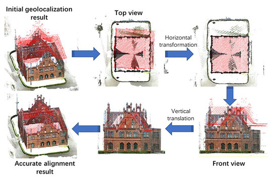
2.3. Accurate Alignment Using NC-CPD

Although the overlaps between ${\widetilde{\mathit{𝓜}}}^{geo}$ and ${\mathit{𝓟}}^{geo}$ in 3D space are hard to find, 2D façade point overlaps can be accurately extracted. We decomposed the accurate alignment into a horizontal transformation and a vertical transformation, as shown in Figure 4.

2.3.1. 2D Façade Point Extraction from the Façade Point Cloud

Although most of the points in the façade point cloud generated from ground images are part of the façade, there are inevitably many noise points (such as trees, lamp-posts, and passers-by), which will adversely affect the alignment. Thus, it is essential to extract the real façade points from the façade point cloud to reduce the adverse effect of the noise points. First, we extracted candidate façade points from the façade point cloud ${\widetilde{\mathit{𝓜}}}^{geo}$ by using the normal vector information. Since the façade point cloud ${\widetilde{\mathit{𝓜}}}^{geo}$ has been aligned in the upright direction, as described in Section 2.1.1, the dot product of normal $N_{p_i}$ of façade point $p_i$ and the upright vector (z-axis) should be zero in an ideal case. Considering the errors during the step of setting the façade point cloud upright, we modified the condition to ${N_{p_i}}^T{\mathit{Z}}_{axis}<0.01$. Then, we refined the candidate façade points by using their neighbor information. For each point $p_i\left(x_i,y_i,z_i\right)$ in the candidate façade points, it is considered a real façade point only if its neighboring points $\left\{n_i\left(x_{ni},y_{ni},z_{ni}\right)\right\}$ within 0.1 m radius satisfy the following conditions:

$$\{\begin{array}{c}\begin{array}{c}\frac{\left(\max \left\{z_i\right\}-\min \left\{z_i\right\}\right)}{2}<\max \left\{z_{ni}\right\}-\min \left\{z_{ni}\right\}\\ \mathrm{card}\left\{n_i\right\}>10\end{array}\end{array}$$

(9)

The above equation means that real façade points should contain enough neighborhood points while these neighborhood points’ height should be distributed within a certain range in the vertical direction. After the two steps, façade points ${\widetilde{\mathit{𝓜}}}_f^{geo}$ are extracted from the façade point cloud ${\widetilde{\mathit{𝓜}}}^{geo}$, and most noise points are removed. Then, we projected all points of ${\widetilde{\mathit{𝓜}}}_f^{geo}$ onto the horizontal plane to obtain 2D façade points ${\widetilde{\mathit{𝓜}}}_{f2D}^{geo}$, as shown in Figure 5C,D.

2.3.2. 2D Boundary Point Extraction of Open LiDAR Data

The alpha shape algorithm [60] is used to find the boundary points from the 2D LiDAR point cloud ${\mathit{𝓟}}_{2D}^{geo}$, which is obtained by projecting LiDAR data into the horizontal plane. First, alpha shapes with all possible alpha radii $\left\{R_i\right|i\in \left(1,N\right)\}$ for ${\mathit{𝓟}}_{2D}^{geo}$ are calculated. Then, we found the critical alpha radius $(R_c$) that creates a single region for the alpha shape. All alpha values above $R_c$ can be extracted as candidate alpha values $\left\{R_k\right\}$. Second, we used a threshold to select one alpha value, $R_f$, from $\left\{R_k\right\}$. Finally, the holes are filled after creating the final alpha shape with alpha value $R_f$. The points in the final alpha shape are considered as the boundary point set ${\mathit{𝓟}}_{b2D}^{geo}$, as shown in Figure 5A,B.

2.3.3. Horizontal Alignment Using NC-CPD

From the previous steps, the 2D boundary points ${\mathit{𝓟}}_{b2D}^{geo}$ and 2D façade points ${\widetilde{\mathit{𝓜}}}_{f2D}^{geo}$ are extracted from the open LiDAR data and the façade point cloud, respectively. The NC-CPD algorithm described in detail in Section 2.2.2 is used to match ${\widetilde{\mathit{𝓜}}}_{f2D}^{geo}$ to ${\mathit{𝓟}}_{b2D}^{geo}$. First, we calculated the initial ${\sigma }^2$ with $\mathit{R}=\mathit{I}, s=1, \mathrm{and} \mathit{t}=\mathbf{0}$. The initial $S$ in Equation (7) is also calculated with ${\mathit{N}}_{{𝓟}_i}$ and the initial ${\mathit{N}}_{{𝓜}_i}$. Then, $P^{old}\left(m|{\mathit{x}}_n\right)$ in Equation (5) is calculated by updating $p\left(\mathit{x}|m\right)$ in Equation (8) using $\mathit{R}, s, \mathit{t}, {\sigma }^2, \mathrm{and} S$. By substituting $P^{old}\left(m|{\mathit{x}}_n\right)$ into Equation (6), the parameters $\mathit{R}, s,\mathit{T}, \mathrm{and} {\sigma }^2$ are updated by minimizing Q in Equation (6). The new $S$ is also updated by using the new ${\mathit{N}}_{{𝓟}_i}^{new}={\mathit{N}}_{{𝓟}_i}{\mathit{R}}^T$. These steps are repeated until Q does not change too much or a certain number of iterations is reached. After applying the final transformation parameters $\left\{\mathit{R}, s, \mathit{t}\right\}$ to the x and y coordinates of ${\widetilde{\mathit{𝓜}}}_{f2D}^{geo}$, an accurately aligned façade point cloud ${\mathit{𝓜}}_{f2D}^{geo}$ for the x and y directions is obtained. The registration process of NC-CPD is described in detail in Algorithm 1.

Algorithm 1: Horizontal Alignment Using Normal Consistency Coherent Point Drift (NC-CPD)
Input: 2D boundary points $\left\{{\mathit{𝓟}}_i\right|i=1,2,\dots N\}$ and the corresponding normal vector ${\mathit{N}}_{{𝓟}_i}$    2D façade points $\left\{{\mathit{𝓜}}_i\right|i=1,2,\dots M\}$ and the corresponding initial normal vector ${\mathit{N}}_{{𝓜}_i}$ Output: Accurate aligned 2D façade points ${\mathit{𝓜}}_{f2D}^{geo}$
1	Initialization: Assign initial parameters: $\mathit{R}=\mathit{I}, s=1, \mathit{t}=\mathbf{0},$
2	Calculate initial ${\sigma }^2:{\sigma }^2=\frac{1}{2NM}{{\displaystyle \sum }}_{n=1}^N{{\displaystyle \sum }}_{m=1}^M||{\mathit{𝓟}}_n-{\mathit{𝓜}}_m{||}^2$,
3	Construct initial normal consistency $S$ in Equation (7)
4	EM optimization. Repeat 5–7 until convergence to obtain the final ${\mathit{R}}_{\mathit{f}}, s_f, {\mathit{t}}_{\mathit{f}}, \mathrm{and} {\sigma }^2$
5	E-step: Update $p\left(m|{\mathit{x}}_n\right)$ with $\mathit{R}, s,\mathit{T}, {\sigma }^2, S$
6	M-step: Solve for the new $\mathit{R}, s, \mathit{T}, {\sigma }^2$ by minimizing Equation (6),
7	Update $S \mathrm{by}\mathrm{using} {\mathit{N}}_{{𝓟}_i}^{new}={\mathit{N}}_{{𝓟}_i}{\mathit{R}}^T$
8	The accurate aligned 2D façade points are given by ${\mathit{𝓜}}_{f2D}^{geo}$ = $s_f{\widetilde{\mathit{𝓜}}}_{f2D}^{geo}{\mathit{R}}_{\mathit{f}}^{\mathit{T}}+{\mathit{t}}_{\mathit{f}}^{\mathit{T}}$

Finally, we update the z coordinates of façade points by applying s and t, and the 3D façade point cloud ${\ddot{\mathit{𝓜}}}^{geo}$ is obtained.

2.3.4. Vertical Alignment

The façade point cloud is accurately aligned to open LiDAR data in the x and y axis direction by the horizontal alignment described in the previous section. A translation, $T_z$, on the vertical direction between ${\ddot{\mathit{𝓜}}}^{geo}$ and ${\mathit{𝓟}}^{geo}$ remains to be calculated. We calculated the optimal $T_z$ by matching corresponding boundary points respectively from ${\mathit{𝓟}}^{geo}$ and ${\ddot{\mathit{𝓜}}}^{geo}$ on the z axis, following these steps: (1) For a point ${\overline{p}}_i\left(x_i,y_i\right)$ of the 2D boundary points ${\mathit{𝓟}}_{b2D}^{geo}$, find its 2D neighbor point set $\{p_1,\dots ,p_i\}$ and $\{q_1,\dots ,q_j\}$ (within a radius of 0.1 m), from ${\mathit{𝓟}}^{geo}$ and ${\ddot{\mathit{𝓜}}}^{geo}$. (2). Find the points $p_m$ and $q_n$ with a maximum value on the z-axis from $\{p_1,\dots ,p_i\}$ and $\{q_1,\dots ,q_j\}$, respectively, then calculate the height difference using the equation $T_i=z_{p_m}-z_{q_n}$. (3). For the other points in ${\mathit{𝓟}}_{b2D}^{geo}$, repeat steps 1 and 2 to obtain the height difference set $\left\{T_1,\dots ,T_i\right\}$. Then, calculate the optimal $T_z$ by fitting height difference set $\left\{T_1,\dots ,T_i\right\}$ to a line using RANSAC. Finally, apply the translation $T_z$ to the z coordinate of ${\ddot{\mathit{𝓜}}}^{geo}$, so that an accurately aligned façade point cloud ${\mathit{𝓜}}^{geo}$ is obtained in the end.

3. Experiments and Discussion

3.1. Dataset Description

So far, there are currently no available benchmark datasets for fusing airborne LiDAR data and façade point clouds generated from images. The proposed method is evaluated on a combined dataset.

1. The open LiDAR data of Dortmund in Germany, which contains three experimental buildings (Rathaus, Lohnhalle, and Verwaltung), are downloaded from a German open data download portal [7]. These open LiDAR data have been geolocated in the ETRS89 reference system using a universal transverse Mercator (UTM) projection with a point density of 25 points/m².

2. Ground images of the three buildings come from a benchmark dataset named “ISPRS benchmark on multi-platform photogrammetry” [61], which can be downloaded from the official website of the ISPRS. These images are captured around buildings using high-resolution digital cameras on the ground. Due to the use of GPS-locating accessories, image shooting positions are recorded in these JPEG formatted images as GPS meta-data. Global coordinates of target centers distributed on the façade of the three buildings are provided for accuracy estimation. The details of these image collections are listed in

Table 1. Details of ground image datasets.

	Rathaus	Lohnhalle	Verwaltung
Number of images	1211	194	351
Façade model points	36,085,050	8,004,604	11,176,836
Capturing device	SONY NEX-7	Canon EOS 600D	Canon EOS 600D
Focal length	16 mm	20 mm	20 mm
Image size (pixel)	4000 × 6000	5184 × 3456	5184 × 3456
Ground resolution	7.6 mm/pixel	3.1 mm/pixel	1.72 mm/pixel
GPS information	✓	✓	✓

.

3.2. Qualitative Analysis

As shown in Figure 6, façade point clouds of Rathaus, Lohnhalle, and Verwaltung (Figure 6B1–B3, respectively) are generated from ground images (Figure 6A1–A3, image sample) using SfM and MVS algorithms in COLMAP [32]. The open LiDAR data of the three buildings is visualized using the height rendering map shown in Figure 6C1–C3. It is evident that there are no overlaps between the open LiDAR data and façade point clouds on the façades, except for Verwaltung, which has a small number of points on the façades. However, from another perspective, open LiDAR data and façade point clouds are complementary. The former lacks structural details on the façades, while the latter lacks roof information.

The initial geolocalization results, which are not entirely accurate due to the low accuracy of GPS, are shown in Figure 6D1–D3 (the red color is assigned to open LiDAR data for better recognition). After performing the accurate alignment step, the façade point clouds and open LiDAR data are aligned well, as shown in Figure 6E1–E3. We also tested the matching of our datasets using the ICP [27] and Normal Distributions Transform (NDT) [62] algorithms, two classical algorithms of point set registration. The visualizing results are shown in Figure 7. Due to a relatively good density of points on the façades, we can see that ICP and NDT achieve a relatively good result in Verwaltung compared with Rathaus and Lohnhalle.

Surface reconstruction (Figure 8) is performed using the method described in [63] to demonstrate the effectiveness of our alignment algorithm. Both completeness and structural details are achieved in the surface reconstruction after accurately aligning the façade point cloud to open LiDAR data.

3.3. Quantitative Analysis

As described in Section 2.2, an iteration process is performed in the EM process to find the optimal alignment result. After less than 30 iterations, the ratio of $Q$ to the initial $Q_0$ quickly declined to 1%, as shown in Figure 9A. Accurate geographical coordinates $\left\{G_i\right\}$ of target centers distributed on the façade, as provided in the dataset of “ISPRS benchmark on multi-platform photogrammetry”, are used for quantitative evaluations of the alignment results, as shown in Figure 9B.

The difference in the final aligned façade point cloud includes deviations from both the façade point cloud generating process and the registration process. It is difficult to estimate the accuracy of the registration process alone. In order to find the optimal geolocated results of the façade point cloud, which include almost no transformation difference, target center registration (TCR) is performed by estimating the similarity transformation $\mathbf{𝓣}\left(\mathit{R},s,\mathit{T}\right)$ between the local coordinates of the manually selected target centers and their provided global coordinates $\left(\left\{G_i\right\}\right)$ using the least-square method. Since the transformation difference is greatly reduced by directly use of high-precision GCPs, transformation difference in the alignment of the façade point cloud using the TCR method comes mainly from the façade point cloud generating process. Thus, the results of the TCR methods can be used as reference values for other registration methods. We applied the proposed method, TCR, ICP, and NDT methods to register initial geolocated façade point cloud (result in Section 2.1) to the airborne LiDAR data. Then, the root mean square error (RMSE), mean error (ME), and standard deviation (SD) of the proposed method are calculated using the following equations:

$$\{\begin{array}{c}RMSE=\sqrt{\frac{1}{N}{\displaystyle \sum _{i=1}^N}{D_i}^2}\\ ME=\frac{1}{N}{\displaystyle \sum _{i=1}^N}{D}_i\\ SD=\sqrt{\frac{1}{N-1}{\displaystyle \sum _{i=1}^N}{\left|D_i-ME\right|}^2}\end{array}$$

(10)

where $D_i$ is the distance between the target center coordinates obtained from the aligned results and their provided global coordinates. The middle 90% of {$D_i$} are used for calculating the RMSE, mean errors, and standard deviation, as shown in

Table 2. The root mean square error (RMSE), the mean error (ME), and the standard deviation (SD) of the proposed method compared with target center registration (TCR), ICP and NDT.

	Targets Qty.	Methods	RMSE (m)	Mean Error (m)	Standard Deviation (m)
Rathaus	20	TCR	0.192	0.164	0.197
		ICP	4.283	3.548	4.280
		NDT	6.814	6.663	1.575
		Proposed method	0.389	0.342	0.304
Verwaltung	40	TCR	0.049	0.030	0.050
		ICP	0.336	0.288	0.300
		NDT	1.700	1.452	1.489
		Proposed method	0.185	0.161	0.173
Lohnhalle	31	TCR	0.188	0.164	0.189
		ICP	10.039	8.537	5.672
		NDT	23.225	22.336	6.495
		Proposed method	0.468	0.380	0.423

.

By analyzing the RMSE value of the different methods in Table 2, we can see that the proposed method significantly improves the accuracy of test datasets compared to the ICP and NDT methods. It is well known that ICP and NDT are effective methods of point set registration with large overlaps. Experiments have shown that ICP and NDT methods cannot handle our datasets, in which almost no overlaps are found. Thus, RMSE value up to 10 m are obtained, except for the Verwaltung dataset, which had a small number of points on the façade parts. While the results are not as good as the result of the TCR method, the proposed method achieves the best accuracy compared to ICP and NDT methods due to the use of similarity on 2D outlines of buildings.

For Rathaus, the far mean capture distance leads to the apparent worst quality of the façade point cloud from captured images (i.e., the most significant RMSE value in the TCR method). Consequently, a relatively large RMSE value appeared in the Rathaus dataset using the proposed method. For the Lohnhalle dataset, we believe the disclosure of images captured around the target building caused relatively apparent deviation in the SfM process, even though the mean capture distance is much closer than that of the Rathaus dataset.

3.4. Robustness Analysis

It is known that different point densities and degrees of noise in the point clouds have a significant impact on the performance of registration. We perform several experiments on point clouds mixed with different degrees of noise and point densities to test the robustness of the proposed method. Figure 10A,B illustrate the registration results achieved by the proposed method under different degrees of noise and point densities.

To evaluate the robustness of the proposed method to point density, we randomly down-sampled the façade point clouds of the Rathaus, Verwaltung, and Lohnhalle data from their original point densities to various reduced densities. The RMSE values evaluated with respect to the target center coordinates at different point densities are given in Figure 10A. It is evident that the proposed method performed well, even at 1% of the original point density, indicating the robustness of the proposed method to different point densities. We attribute the robustness of our approach to different point densities to the use of the 2D similarity of building outlines in the registration between two sources of point clouds.

To evaluate the robustness of the proposed method to noise, Gaussian noise with different standard deviations (1, 2, 3, 4, and 5 cm) is added to the point cloud data. The RMSE values evaluated with respect to the target center coordinates under different levels of noise are shown in Figure 10B. Even when Gaussian noise with a standard deviation of 5 cm is added to the point cloud, the proposed method achieved fine and stable accuracy. This indicates that the proposed method is very robust to different levels of noise. We attribute the robustness of our approach to different degrees of noise to the use of the probabilistic method in the accurate alignment method.

3.5. Expandability for Crowdsourcing Images

To test the expandability for crowdsourcing images, we have tested the proposed method on crowdsourcing images of several buildings in our campus acquired by smartphones and digital cameras. Experiments show that if most of the façade point cloud can be successfully restored from crowdsourcing images, the proposed fusion approach is effective, as shown in Figure 11.

Therefore, successfully reconstructing the facade point cloud from these images through, e.g., COLMAP is a prerequisite for our approach.

But sometimes COLMAP fails in the SfM procedure because the following problems are common to crowdsourcing images: (1) missing photos in some locations; (2) occlusion of trees; (3) repetitive structures on the façade (e.g., similar windows); and (4) failure to match images with large differences (e.g., capture angle and illumination). The above cases will result in failure to generate the façade point cloud, which will make the proposed method ineffective. Consequently, ensuring complete image coverage and good image quality is beneficial to extend the proposed method to crowdsourcing images.

4. Conclusions

This paper presents an accurate and efficient approach for improving building façade details of open LiDAR data using ground images. The essence of the proposed approach is the fusion of the façade point clouds generated from ground images and open LiDAR data, between which there are very limited overlaps and it is different from the common situation with adequate overlap. By using a two-step strategy, the scale, translation, and rotation differences are greatly relieved after initial geolocalization of the façade point cloud using GPS meta-data. 2D overlapping points on the outline of buildings are effective for the registration of the façade point cloud and airborne point cloud than 3D overlapping points, which can hardly be found between the two different sources of point clouds. We decompose the registration of the two-point cloud into a horizontal and vertical transformations instead of 3D registration directly. The proposed NC-CPD inherits the noise robustness property of the original CPD algorithm, which is a probabilistic-based point set registration algorithm. At the same time, it can handle the registration with structural ambiguities of buildings by introducing normal consistency into the original CPD algorithm.

Both completeness and structural details of buildings in open LiDAR data are significantly improved after accurate alignment so that a complete and full-resolution city building model and other applications can be achieved. Experiments have shown that classic registration methods, such as ICP and NDT, cannot handle this situation. Compared with ICP and NDT, the proposed method achieves 2 to 10 times higher registration accuracy.

References

1. NYC Open Data. Available online: https://opendata.cityofnewyork.us/ (accessed on 14 October 2018).
2. Open Data DC. Available online: http://opendata.dc.gov/ (accessed on 14 October 2018).
3. Open Data of Canada. Available online: https://open.canada.ca/en/open-data (accessed on 14 October 2018).
4. INSPIRE Directive. Directive 2007/2/EC of the European Parliament and of the Council of 14 March 2007 establishing an Infrastructure for Spatial Information in the European Community (INSPIRE). Off. J. Eur. Union 2007, L 108, 1–14. [Google Scholar]
5. European Data Portal. Available online: https://data.europa.eu (accessed on 14 October 2018).
6. Scottish Remote Sensing Portal. Available online: https://remotesensingdata.gov.scot/ (accessed on 14 October 2018).
7. Open NRW. Available online: https://open.nrw/open-data/ (accessed on 14 October 2018).
8. Langheinrich, M. Evaluation of Gmsh Meshing Algorithms in Preparation of High-Resolution Wind Speed Simulations in Urban Areas. Int. Arch. Photogramm. Remote Sens. Spat. Inf. Sci. 2018, 42, 559–564. [Google Scholar] [CrossRef]
9. Kersting, N. Open Data, Open Government und Online Partizipation in der Smart City. Vom Informationsobjekt über den deliberativen Turn zur Algorithmokratie? In Staat, Internet und Digitale Gouvernementalität; Springer: Wiesbaden, Germany, 2018; pp. 87–104. [Google Scholar]
10. Degbelo, A.; Trilles, S.; Kray, C.; Bhattacharya, D.; Schiestel, N.; Wissing, J.; Granell, C. Designing semantic application programming interfaces for open government data. eJ. eDemocr. Open Gov. 2016, 8, 21–58. [Google Scholar]
11. Luebke, D.; Reddy, M.; Cohen, J.D.; Varshney, A.; Watson, B.; Huebner, R. Level of Detail for 3D Graphics: Application and Theory; Morgan Kaufmann: Burlington, MA, USA, 2002; p. 431. [Google Scholar]
12. Hobrough, G.L. Automatic stereo plotting. Photogramm. Eng. 1959, 25, 763–769. [Google Scholar]
13. Schenk, T. Towards automatic aerial triangulation. ISPRS J. Photogramm. Remote Sens. 1997. [Google Scholar] [CrossRef]
14. Cramer, M.; Stallmann, D.; Haala, N. Direct Georeferencing Using Gps/Inertial Exterior Orientations for Photogrammetric Applications. Int. Arch. Photogramm. Remote Sens. 2000, 33, 198–205. [Google Scholar]
15. Krupnik, A. Multiple-Patch Matching in the Object Space for Aerotriangulation. Ph.D. Thesis, The Ohio State University, Columbus, OH, USA, 1994; 93p. [Google Scholar]
16. Agarwal, S.; Snavely, N.; Simon, I.; Seitz, S.M.; Szeliski, R. Building Rome in a day. In Proceedings of the 2009 IEEE 12th International Conference on Computer Vision, Kyoto, Japan, 29 September–2 October 2009; pp. 72–79. [Google Scholar] [CrossRef]
17. Wan, G.; Snavely, N.; Cohen-Or, D.; Zheng, Q.; Chen, B.; Li, S. Sorting unorganized photo sets for urban reconstruction. Graph. Models 2012, 74, 14–28. [Google Scholar] [CrossRef]
18. Simon, I.; Snavely, N.; Seitz, S.M. Scene Summarization for Online Image Collections. In Proceedings of the 11th IEEE International Conference on Computer Vision, Rio de Janeiro, Brazil, 14–21 October 2007; pp. 1–8. [Google Scholar] [CrossRef]
19. Zhang, L.; Gruen, A. Multi-image matching for DSM generation from IKONOS imagery. ISPRS J. Photogramm. Remote Sens. 2006, 60, 195–211. [Google Scholar] [CrossRef]
20. Hirschmüller, H. Stereo processing by semiglobal matching and mutual information. IEEE Trans. Pattern Anal. Mach. Intell. 2008, 30, 328–341. [Google Scholar] [CrossRef] [PubMed]
21. Furukawa, Y.; Ponce, J. Accurate, dense, and robust multiview stereopsis. IEEE Trans. Pattern Anal. Mach. Intell. 2010, 32, 1362–1376. [Google Scholar] [CrossRef] [PubMed]
22. Vu, H.-H.; Labatut, P.; Pons, J.-P.; Keriven, R. High accuracy and visibility-consistent dense multiview stereo. IEEE Trans. Pattern Anal. Mach. Intell. 2012, 34, 889–901. [Google Scholar] [CrossRef] [PubMed]
23. Schonberger, J.L.; Frahm, J.-M. Structure-from-Motion Revisited. In Proceedings of the 2016 IEEE Conference on Computer Vision and Pattern Recognition (CVPR), Las Vegas, NV, USA, 26 June–1 July 2016. [Google Scholar]
24. Moulon, P.; Monasse, P.; Perrot, R.; Marlet, R. OpenMVG: Open multiple view geometry. In International Workshop on Reproducible Research in Pattern Recognition; Springer: Berlin, Germany, 2016; pp. 60–74. [Google Scholar]
25. Wu, C. Towards Linear-Time Incremental Structure from Motion. In Proceedings of the 2013 International Conference on 3D Vision—3DV, Seattle, WA, USA, 29 June–1 July 2013; pp. 127–134. [Google Scholar] [CrossRef]
26. Böhm, J.; Haala, N. Efficient integration of aerial and terrestrial laser data for virtual city modeling using lasermaps. In Proceedings of the ISPRS Workshop Laser Scanning 2005, Enschede, The Netherlands, 12–14 September 2005; pp. 192–197. [Google Scholar]
27. Besl, P.J.; McKay, N.D. A Method for Registration of 3-D Shapes. IEEE Trans. Pattern Anal. Mach. Intell. 1992, 14, 239–256. [Google Scholar] [CrossRef]
28. Boulaassal, H.; Landes, T.; Grussenmeyer, P. Reconstruction of 3D Vector Models of Buildings by Combination of Als, Tls and Vls Data. ISPRS Int. Arch. Photogramm. Remote Sens. Spat. Inf. Sci. 2012, XXXVIII-5/W16, 239–244. [Google Scholar] [CrossRef]
29. Muenkel, C.; Leiterer, U.; Dier, H.D. Scanning the troposphere with a low-cost eye-safe lidar. In Proceedings of the Environmental Sensing and Applications, Munich, Germany, 14–18 June 1999. [Google Scholar]
30. Münkel, C.; Emeis, S.; Schäfer, K.; Brümmer, B. Improved near-range performance of a low-cost one lens lidar scanning the boundary layer. In Proceedings of the Remote Sensing of Clouds and the Atmosphere XIV, Berlin, Germany, 31 August–3 September 2009. [Google Scholar]
31. Tomoiagäf, T.; Predoi, C.; CoåŸEreanu, L. Indoor Mapping Using Low Cost LIDAR Based Systems. Appl. Mech. Mater. 2016, 841, 198–205. [Google Scholar] [CrossRef]
32. Shan, Q.; Wu, C.; Curless, B.; Furukawa, Y.; Hernandez, C.; Seitz, S.M. Accurate geo-registration by ground-to-aerial image matching. In Proceedings of the 2014 2nd International Conference on 3D Vision, Tokyo, Japan, 8–11 December 2014; pp. 525–532. [Google Scholar] [CrossRef]
33. Rönnholm, P.; Honkavaara, E.; Litkey, P.; Hyyppä, H.; Hyyppä, J. Integration of Laser Scanning and Photogrammetry. Int. Arch. Photogramm. Remote Sens. Spat. Inf. Sci. 2007, XXXVI-3/W5, 355–362. [Google Scholar] [CrossRef]
34. Becker, S.; Haala, N. Combined feature extraction for facade reconstruction. In Proceedings of the ISPRS Workshop on Laser Scanning 2007 and SilviLaser 2007, Espoo, Finlan, 12–14 September 2007. [Google Scholar]
35. González-Aguilera, D.; Rodríguez-Gonzálvez, P.; Gómez-Lahoz, J. An automatic procedure for co-registration of terrestrial laser scanners and digital cameras. ISPRS J. Photogramm. Remote Sens. 2009. [Google Scholar] [CrossRef]
36. Rönnholm, P.; Haggrén, H. Registration of Laser Scanning Point Clouds and Aerial Images Using Either Artifical or Natuarl Tie Featurs. ISPRS Ann. Photogramm. Remote Sens. Spat. Inf. Sci. 2012, 3, 63–68. [Google Scholar] [CrossRef]
37. Stamos, I.; Allen, P.K. Geometry and texture recovery of scenes of large scale. Comput. Vis. Image Underst. 2002, 88, 94–118. [Google Scholar] [CrossRef]
38. Inglot, A.; Tysiac, P. Airborne Laser Scanning Point Cloud Update by Used of the Terrestrial Laser Scanning and the Low-Level Aerial Photogrammetry. In Proceedings of the 2017 Baltic Geodetic Congress (BGC Geomatics), Gdansk, Poland, 22–25 June 2017; pp. 34–38. [Google Scholar] [CrossRef]
39. Klapa, P.; Mitka, B.; Zygmunt, M. Application of Integrated Photogrammetric and Terrestrial Laser Scanning Data to Cultural Heritage Surveying. IOP Conf. Ser. Earth Environ. Sci. 2017, 95. [Google Scholar] [CrossRef]
40. Böhm, J.; Becker, S.; Haala, N. Model refinement by integrated processing of laser scanning and photogrammetry. In Proceedings of the Proceedings of 2nd International workshop on 3D Virtual Reconstruction and Visualization of Complex Architectures (3D-Arch), Zurich, Switzerland, 12–13 July 2007. [Google Scholar]
41. Mastin, A.; Kepner, J.; Fisher, J. Automatic registration of LIDAR and optical images of urban scenes. In Proceedings of the 2009 IEEE Computer Society Conference on Computer Vision and Pattern Recognition Workshops, CVPR Workshops 2009, Miami, FL, USA, 20–25 June 2009. [Google Scholar]
42. Wang, L.; Neumann, U. A robust approach for automatic registration of aerial images with untextured aerial LiDAR data. In Proceedings of the 2009 IEEE Computer Society Conference on Computer Vision and Pattern Recognition Workshops, CVPR Workshops 2009, Miami, FL, USA, 20–25 June 2009. [Google Scholar]
43. Rueckert, D.; Sonoda, L.I.; Hayes, C.; Hill, D.L.; Leach, M.O.; Hawkes, D.J. Nonrigid registration using free-form deformations: Application to breast MR images. IEEE Trans. Med. Imaging 1999, 18, 712–721. [Google Scholar] [CrossRef]
44. El-Hakim, S.F.; Beraldin, J.A.; Picard, M.; Godin, G. Detailed 3D reconstruction of large-scale heritage sites with integrated techniques. IEEE Comput. Graph. Appl. 2004, 24, 21–29. [Google Scholar] [CrossRef] [PubMed]
45. Goshtasby, A.A. 2-D and 3-D Image Registration: For Medical, Remote Sensing, and Industrial Applications; John Wiley & Sons: Hoboken, NJ, USA, 2005; ISBN 0471724262. [Google Scholar]
46. Myronenko, A.; Song, X. Point set registration: Coherent point drifts. IEEE Trans. Pattern Anal. Mach. Intell. 2010, 32, 2262–2275. [Google Scholar] [CrossRef] [PubMed]
47. Maiseli, B.; Gu, Y.; Gao, H. Recent developments and trends in point set registration methods. J. Vis. Commun. Image Represent. 2017, 46, 95–106. [Google Scholar] [CrossRef]
48. Yang, B.; Dong, Z.; Liang, F.; Liu, Y. Automatic registration of large-scale urban scene point clouds based on semantic feature points. ISPRS J. Photogramm. Remote Sens. 2016, 113, 43–58. [Google Scholar] [CrossRef]
49. Gold, S.; Rangarajan, A.; Lu, C.P.; Pappu, S.; Mjolsness, E. New algorithms for 2D and 3D point matching: Pose estimation and correspondence. Pattern Recognit. 1998. [Google Scholar] [CrossRef]
50. Baba, B.J.; Vemuri, C. A robust algorithm for point set registration using mixture of Gaussians. In Proceedings of the IEEE International Conference on Computer Vision, Beijing, China, 17–21 October 2005. [Google Scholar]
51. Brun, A.; Westin, C. Robust Generalized Total Least Squares. Miccai 2004, 234–241. [Google Scholar] [CrossRef]
52. Chetverikov, D.; Stepanov, D.; Krsek, P. Robust Euclidean alignment of 3D point sets: The trimmed iterative closest point algorithm. Image Vis. Comput. 2005, 23, 299–309. [Google Scholar] [CrossRef]
53. Stewart, C.V.; Tsai, C.L.; Roysam, B. The dual-bootstrap iterative closest point algorithm with application to retinal image registration. IEEE Trans. Med. Imaging 2003, 22, 1379–1394. [Google Scholar] [CrossRef] [PubMed] [Green Version]
54. Kaneko, S.; Kondo, T.; Miyamoto, A. Robust matching of 3D contours using iterative closest point algorithm improved by M-estimation. Pattern Recognit. 2003, 36, 2041–2047. [Google Scholar] [CrossRef] [Green Version]
55. Campbell, D.; Petersson, L. An adaptive data representation for robust point-set registration and merging. In Proceedings of the IEEE International Conference on Computer Vision (ICCV), Santiago, Chile, 7–13 December 2015; pp. 4292–4300. [Google Scholar] [CrossRef]
56. Yang, C.; Medioni, G. Object modelling by registration of multiple range images. Image Vis. Comput. 1992. [Google Scholar] [CrossRef]
57. Fischler, M.A.; Bolles, R.C. Random sample consensus: A paradigm for model fitting with applications to image analysis and automated cartography. Commun. ACM 1981, 24, 381–395. [Google Scholar] [CrossRef]
58. Zandbergen, P.A.; Barbeau, S.J. Positional accuracy of assisted GPS data from high-sensitivity GPS-enabled mobile phones. J. Navig. 2011. [Google Scholar] [CrossRef]
59. GPS Accuracy. Available online: https://www.gps.gov/systems/gps/performance/accuracy/ (accessed on 14 October 2018).
60. Edelsbrunner, H.; Mücke, E.P. Three-dimensional alpha shapes. ACM Trans. Graph. 1994, 13, 43–72. [Google Scholar] [CrossRef] [Green Version]
61. Nex, F.; Remondino, F.; Gerke, M.; Przybilla, H.-J.; Bäumker, M.; Zurhorst, A. ISPRS Benchmark for multi-platform photogrammetry. ISPRS Ann. Photogramm. Remote Sens. Spat. Inf. Sci. 2015, 2, 135–142. [Google Scholar] [CrossRef]
62. Magnusson, M. The Three-Dimensional Normal-Distributions Transform—An Efficient Representation for Registration, Surface Analysis, and Loop Detection. Renew. Energy 2009, 28, 655–663. [Google Scholar]
63. Kazhdan, M.; Hoppe, H. Screened poisson surface reconstruction. ACM Trans. Graph. 2013, 32, 29. [Google Scholar] [CrossRef]
Figure 1. The overview of the proposed method.
Remotesensing 11 00420 g001
Figure 2. An overview of the initial geolocalization process. (A) Camera positions calculated using SfM (red) (B) and camera GPS meta-information (green points) aligned using a random sample consensus (RANSAC)-based similarity transformation. Simultaneously, the façade point cloud (textured points) is aligned to the point cloud of the building from the open LiDAR data (blue points) by applying the calculated 2D similarity transformation parameters in the horizontal direction and a vertical translation. (C) The alignment results.
Remotesensing 11 00420 g002
Figure 3. Illustration of the alignment procedure. (A) The 2D boundary points from LiDAR (red points) and their normal N 𝓟 i (green lines with arrows). (B) The 2D façade points (blue points) and their normal N 𝓜 i (blue lines with arrow). (C) An incorrect alignment result due to ambiguities, as seen by the large difference between the normal directions in the overlapping part of the two point clouds. (D) A correct alignment result as seen by the high similarity between the normal directions of points in the overlapping part.
Remotesensing 11 00420 g003
Figure 4. Overview of the proposed accurate alignment process. Red points are building point cloud from open LiDAR data. Textured points are façade point cloud generated from ground images.
Remotesensing 11 00420 g004
Figure 5. Results of 2D façade point extraction and 2D boundary point extraction. (A) The open LiDAR data. (B) The boundary points (top view) extracted from open LiDAR data. (C) The façade point cloud. (D) The façade boundary points (top view) extracted from the façade point cloud.
Remotesensing 11 00420 g005
Figure 6. Datasets for evaluating the proposed method. From top to bottom, the different rows show the following results for Rathaus, Verwaltung, and Lohnhalle: (A) ground images, (B) façade point clouds, (C) open LiDAR data (height rendering), (D) coarse alignment results, and (E) accurate alignment results.
Remotesensing 11 00420 g006
Figure 7. Fusion results of the proposed method compared with the ICP and NDT methods. Red points are building point cloud from open LiDAR data. Textured points are façade point cloud generated from ground images.
Remotesensing 11 00420 g007
Figure 8. Poisson surface reconstruction results from: (A) open LiDAR data. (B) a façade point cloud generated from ground images. (C) the fusion point cloud of open LiDAR data and the façade point cloud.
Remotesensing 11 00420 g008
Figure 9. (A) Likelihood function Q relative to the initial value Q0 as a function of the number of iterations. (B) Illustration of ground targets.
Remotesensing 11 00420 g009
Figure 10. Robustness analysis of the proposed method. In figure (A), we randomly down-sampled the façade point clouds of the Rathaus, Verwaltung, and Lohnhalle data from their original point densities to various reduced densities in order to estimate the robustness to point density. In figure (B), we added Gaussian noise with different standard deviations (1, 2, 3, 4, and 5 cm) to the point cloud data to estimate the robustness to noise.
Remotesensing 11 00420 g010
Figure 11. Fusion results of the proposed method tested on crowdsourcing images. Red points are building point cloud from airborne LiDAR data. Textured points are façade point cloud generated from ground images of several buildings on our campus acquired by smartphones and digital cameras.
Remotesensing 11 00420 g011