Assimilation of SMOS Sea Surface Salinity in the Regional Ocean Model for South China Sea

Abstract

Ocean salinity has an important impact on marine environment simulations. The Soil Moisture and Ocean Salinity (SMOS) mission is the first satellite in the world to provide large-scale global salinity observations of the oceans. Salinity remote sensing observations in the open ocean have been successfully applied in data assimilations, while SMOS salinity observations contain large errors in the coastal ocean (including the South China Sea (SCS)) and high latitudes and cannot be effectively applied in ocean data assimilations. In this paper, the SMOS salinity observation data are corrected with the Generalized Regression Neural Network (GRNN) in data assimilation preprocessing, which shows that after correction, the bias and root mean square error (RMSE) of the SMOS sea surface salinity (SSS) compared with the Argo observations can be reduced from 0.155 PSU and 0.415 PSU to −0.003 PSU and 0.112 PSU, respectively, in the South China Sea. The effect is equally significant in the northwestern Pacific region. The preprocessed salinity data were applied to an assimilation in a coastal region for the first time. The six groups of assimilation experiments set in the South China Sea showed that the assimilation of corrected SMOS SSS can effectively improve the upper ocean salinity simulation.

1. Introduction

Ocean data assimilation can provide better initial and boundary conditions for ocean numerical simulations, thus improving the forecasts of ocean numerical models. Early ocean data assimilation mainly involves univariate assimilation, i.e., only temperature profiles are assimilated and improved [1,2,3,4]. The adjustment of other variables depends entirely on model dynamics which may deteriorate the density field [5]. Considering the importance of salinity on the density field [6,7], methods of simultaneously assimilating the temperature and salinity fields have been gradually proposed. In regions lacking salinity observations, the salinity field is adjusted based on the temperature/salinity(T/S) relationship [8,9]. Before 2009, only in situ salinity profile data were available [10]. Despite the high accuracy and vertical resolution, the spatial distribution of salinity observation data was sparse due to the difficulty and expense of obtaining in situ observations [11]. Satellite remote sensing of salinity enables the acquirement of global scale observations on the sea surface, making up for the sparseness of in situ observations, and providing a new observational method for salinity data assimilation.

In a study of sea surface salinity (SSS) assimilation, Hackert et al. [12] simultaneously assimilated the gridded SSS and subsurface temperature from in situ observations using optimal interpolation in a coupled model. The results showed that the assimilation of the SSS and subsurface temperature can improve the El Nino Southern Oscillation (ENSO)’s forecasting ability better than only assimilating the subsurface temperature. Hackert et al. [13] compared the effects of assimilating Aquarius SSS and in situ SSS and found that satellite observations had a better effect due to the higher observation density. Chakraborty et al. [14] used Singular Evolutive Extended Kalman (SEEK) to assimilate the Aquarius SSS into a global ocean model and showed that the SSS assimilation could improve the sea surface current field and assimilation of the sea surface temperature (SST) combined with the SSS, and a better result was yielded. In terms of the salinity field simulation effect, the assimilation of satellite SSS observations not only improves the sea surface salinity simulation but also improves simulation of the salinity field in the upper layers of the open ocean [15,16]. However, the SSS assimilation effect depends significantly on SSS data quality. Assimilation of SSS data with a lower accuracy may lead to worse salinity fields [17].

The Soil Moisture and Ocean Salinity (SMOS) [18] satellite was launched in 2009 and remains ongoing. Although satellites can provide abundant SSS data, the observations contain large errors and cannot be directly applied to the assimilation system used in coastal areas (such as the China Sea and Japan Sea) or at high latitudes [16,17,19,20,21]. Among the previous studies, Kohl et al. [17] compared the SMOS dataset produced by the University of Hamburg based on the reprocessed ESA’s L2 product (Version 5.50) with EN3 v2a data and they found that the root mean square error (RMSE) is typically approximately 1 g/kg but can reach 3 g/kg in a few locations in the coastal regions and at high latitudes. Lu et al. [16] compared five SMOS L3/L4 products produced by different retrieval algorithms with Argo salinity measurements at 6 m; the large RMSE of five products compared with Argo data in coastal regions can be partially explained by Ratio Frequency Interference (RFI) and the land–sea contamination (LSC), and only a few observations were assimilated in the model after quality control (see Figure 2 in [16]).Therefore, it is worthwhile to study the assimilation of satellite SSS into a model for these regions.

The SMOS L3 SSS product released by the Barcelona Expert Center (BEC) is retrieved using a debiased non-Bayesian method to remove the systematic part of RFI-induced and LSC-induced errors of the retrieved salinities [22]. The advantage of this product over other SSS products is that the dataset contains observations from both coastal regions and high latitudes. However, notably, the SSS data in these areas still contain large errors, which is similar to that for the previous products [16] used in the coastal region. Previous studies have shown that the employment of Neural Networks (NNs) is a good method for retrieving and correcting remote sensing data. Vernieres et al. [15] proposed using a Feed Forward Artificial Neural Network (FFANN) to correct the Aquarius SSS prior to assimilation. The bias and RMSE of the assimilation experiment results are significantly reduced compared with the in situ observations. Ammar et al. [23] proposed a series of NNs based on different incidence angles to retrieve the SSS through SMOS temperature brightness. NNs have been applied widely in remote sensing field so that the Generalized Regression Neural Network (GRNN) is proposed in this study to correct the SMOS SSS in the preprocessing process.

To assimilate SMOS SSS into the ocean model and improve the SSS simulation, the Generalized Regression Neural Network is proposed to correct the SSS of the BEC L3 objective analysis data set based on the characteristic that GRNN can work with a dataset with low accuracy. Then, the corrected SSS data are assimilated into a regional ocean model with a four-dimensional variational assimilation (4DVAR) method. The differences between the model simulation of SSS before and after assimilation are compared, and the SSS data assimilation impacts on the subsurface salinity are studied.

The structure of this paper is as follows: In the second section, the SSS data assimilation preprocessing based on GRNN is introduced. In Section 3, the model, the 4DVAR method, data used in the assimilation and the setting of the assimilation experiments are outlined. The analysis of the assimilation results is described in Section 4. Finally, the discussion and conclusions are presented in Section 5 and Section 6, respectively.

2. SMOS Salinity Observations Preprocessing Based on GRNN

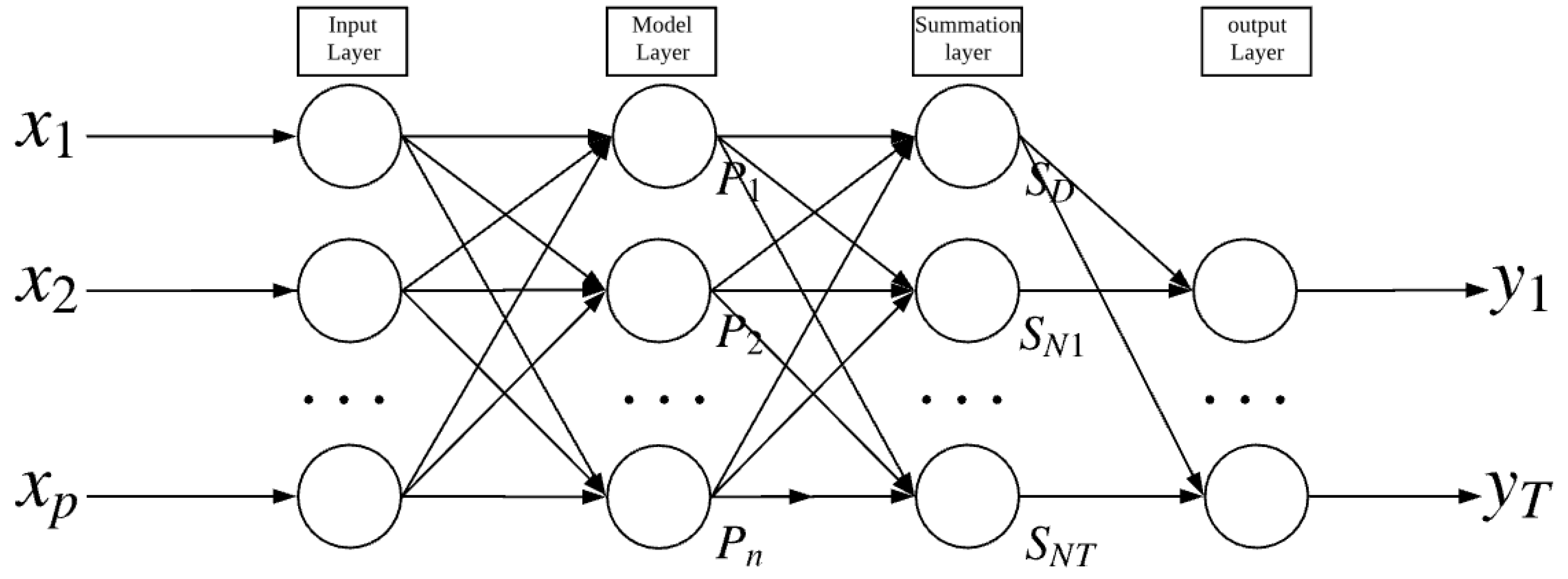
2.1. The Theory and Structure of GRNN

The GRNN, with a posterior condition defined by the sample dataset, estimates the joint probability density function between variables based on nonparametric regression. The GRNN output is based on the maximum probability principle. GRNN has an advantage in nonlinear approximation [24,25] and performs well under conditions of low data accuracy, therefore being suitable for the correction of satellite SSS. Suppose X and Y are two sets of random variables with a joint probability density of $\mathrm{f}\left(\mathrm{X},\mathrm{Y}\right)$, if the value of X is known as $X_0$, the regression of Y versus $X_0$ is as follows:

$$\mathrm{E}\left(\mathrm{Y}|X_0\right)=\mathrm{Y}\left(X_0\right)=\frac{{{\displaystyle \int }}_{-\infty }^{\infty }Yf\left(X_0,\mathrm{Y}\right)\mathrm{dY}}{{{\displaystyle \int }}_{-\infty }^{\infty }f\left(X_0,Y\right)dY}$$

(1)

$\mathrm{Y}\left(X_0\right)$ is the predicted value of Y when the input is $X_0$. The focus of generalized regression is the estimation of the joint probability density function $\mathrm{f}\left(X_0,\mathrm{Y}\right)$. Parzen nonparametric estimation is the method commonly used to estimate $\mathrm{f}\left(X_0,\mathrm{Y}\right)$. Given the sample dataset ${\left\{X_i,Y_i\right\}}_{i=1}^n$, according to the Parzen nonparametric estimation method, $\mathrm{f}\left(X_0,\mathrm{Y}\right)$ can be estimated with the following formula:

$$\mathrm{f}\left(X_0,\mathrm{Y}\right)=\frac{1}{n{\left(2\pi \right)}^{\frac{p+1}{2}}{\sigma }^{p+1}}{\displaystyle \sum }_{i=1}^n{e}^{-d\left(X_0,X_i\right)}{e}^{-d\left(Y(X_0\right),Y_i)}$$

(2)

$$\mathrm{d}\left(X_0,X_i\right)=\frac{{\left(X_0-X_i\right)}^T\left(X_0-X_i\right)}{2{\sigma }^2};\mathrm{d}\left(X_0,Y_i\right)=\frac{{\left(\mathrm{Y}\left(X_0\right)-Y_i\right)}^2}{2{\sigma }^2}$$

(3)

where $\mathrm{d}\left(X_0,X_i\right)$ is the square of Euclidean distance between the input vector $X_0$ and the sample $X_i$.

According to the joint probability density and combining the formulas (1)–(3) the regression of Y versus $X_0$ can be expressed as follows:

$$\mathrm{Y}\left(X_0\right)=\frac{{{\displaystyle \sum }}_{i=1}^{n}Y{e}^{-d\left(X_0,X_i\right)}}{{{\displaystyle \sum }}_{i=1}^n{e}^{-d\left(X_0,X_i\right)}}$$

(4)

where n is the sample dataset size and p is the dimension of X. The only parameter in GRNN is the smoothing factor $\mathsf{\sigma }$. When $\mathsf{\sigma }$ is too large, Y$(X_0$) approximates the mean value of Y in the sample set, indicating that the model is underfitting. When $\mathsf{\sigma }$ is too small, Y$(X_0$) is close to the training set, indicating that the model is overfitting. Therefore, the smoothing factor and the selection of the training set are very important. In this paper, the cross-validation method is used to choose the optimal $\mathsf{\sigma }$ and the optimal training set. The algorithm is shown in Figure 1.

2.2. Data Description

The following datasets were used in the GRNN correction and results verification. (1) The Argo data were obtained from the France Coriolis Argo global data assembly center (ftp://ftp.ifremer.fr/ifremer/argo/). The salinities used in this study are the salinities corrected by delayed-mode in the Argo products and we only use the data with a quality flag equal to 1 [26]. (2) SMOS SSS is the latest 9-day average level3 global product released by the BEC (www.smos-bec.icm.csic.es), and the horizontal resolution is 0.25° × 0.25°. The product is derived from the SMOS L1B TBs v620 dataset considering the SSS inversion of regions with high-level land-sea pollution or sparse observations [22]. (3) SST is obtained from NOAA’s optimal interpolated SST (National Ocean and Atmospheric Administration’s (NOAA’s) National Climate Data Center (NCDC). Its spatial resolution is 0.25° × 0.25° and the temporal resolution is 1 day [27] (ftp://eclipse.ncdc.noaa.gov). (4) The altimeter sea level anomaly (SLA) data are provided by Ssalto/Duacs and distributed by Archiving, Validation, and Interpretation of Satellite Oceanographic (Aviso) with support from CNES (http://www.aviso.oceanobs.com/duacs/). (5) The In Situ Analysis System (ISAS, version ISAS-15) gridded data were used to examine the results. The data set is published by SEA scieNtific Open data Edition (SEANOE) [28,29], with a horizontal resolution of 0.5° × 0.5° and 152 layers in the vertical direction (https://www.seanoe.org/).

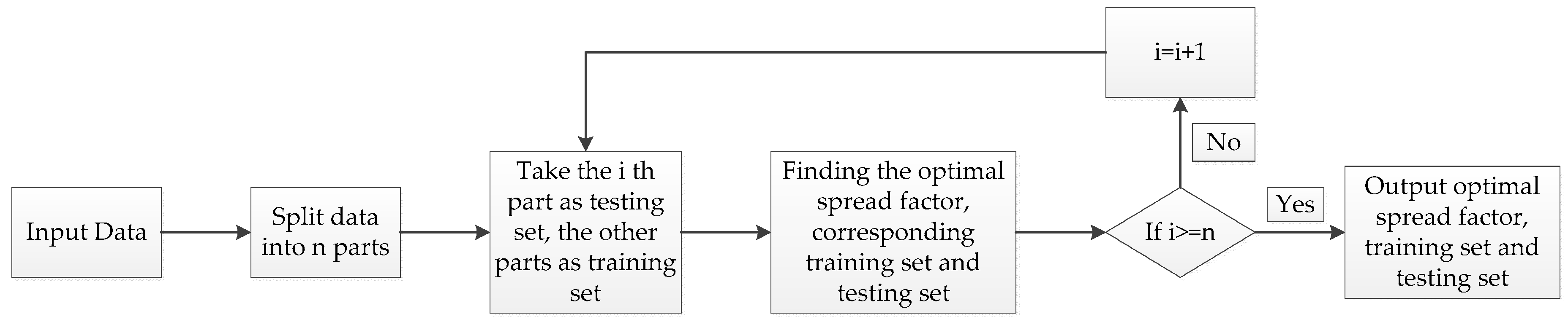
2.3. Neural Network Construction and Model tTraining

The GRNN input can be expressed as follows:

$$X^T=\left(Longitude,Latitude,Time,SST,SLA,SMOS\_SSS\right)$$

(5)

where SST and SLA are two important properties of the ocean [30], and SST is an important variable in the SSS retrieval process [31]. $\left(Longitude,Latitude,Time\right)$ represent the spatial and temporal variabilities. The surface observations (~5 m) of Argo floats are taken as the truth due to the high level of accuracy. The latitude, longitude, and time in the GRNN input layer are the latitude, longitude, and observation month for the Argo floats, respectively. The temporal resolution is 1 day and the spatial resolution is 0.25° × 0.25°. The satellite data (SSS, SST, and SLA) are interpolated to the locations of Argo floats to ensure consistency between the satellite data and Argo data. The GRNN structure is shown in Figure 2. ($x_1,x_2,\dots ,x_p$) and ($y_1,\dots ,y_T$) are the GRNN input and output, respectively. In this study, ($y_1,\dots ,y_T$) is the corrected SSS with $\mathrm{T}=1$. The input layer neurons number is the dimension number of the input vector, which here is 6. Each input neuron is responsible for passing variables to the model layer. The number of model layer neurons is equal to the number of samples; each neuron corresponds to a different sample. The model layer neuron transfer function is the exponential form of $\mathrm{d}\left(X_0,X_i\right)$:

$$P_i=\exp (-\frac{{\left(X_0-X_i\right)}^T\left(X_0-X_i\right)}{2{\sigma }^2})$$

(6)

There are two types of neurons in the summation layer, one of which has only one neuron, and it arithmetically sums the output of all model layer neurons; its transfer function is:

$$S_D={\displaystyle \sum }_{i=1}^n{P}_i$$

(7)

The number of the other type of neurons (called weight neurons) is the dimension number of output vector Y and its transfer function can be expressed as:

$$S_{Nj}={\displaystyle \sum }_{i=1}^n{y}_{ij}{P}_i\hspace{1em}\hspace{1em}j=1,2,\dots T$$

(8)

where $y_{ij}$ is the jth component of sample $Y_i$. Each neuron in the output layer corresponds to an element of $\mathrm{Y}\left(X_0\right)$:

$$y_j=\frac{S_{Nj}}{S_D} j=1,2,\dots T$$

(9)

In this study, there are only one weight summation layer neuron and one output layer neuron.

The model region (105°E–135°E, 12°N–30°N) has been divided into the South China Sea (SCS) and western Pacific due to the differences in the hydrographic features and water masses. In each region, the GRNN model is constructed based on the structure of the bias and RMSE compared with the ISAS-15 monthly average data. The data during 2011 and 2014 are set as the sample set and the implement of GRNN is based on MATLAB through the built-in function newgrnn.

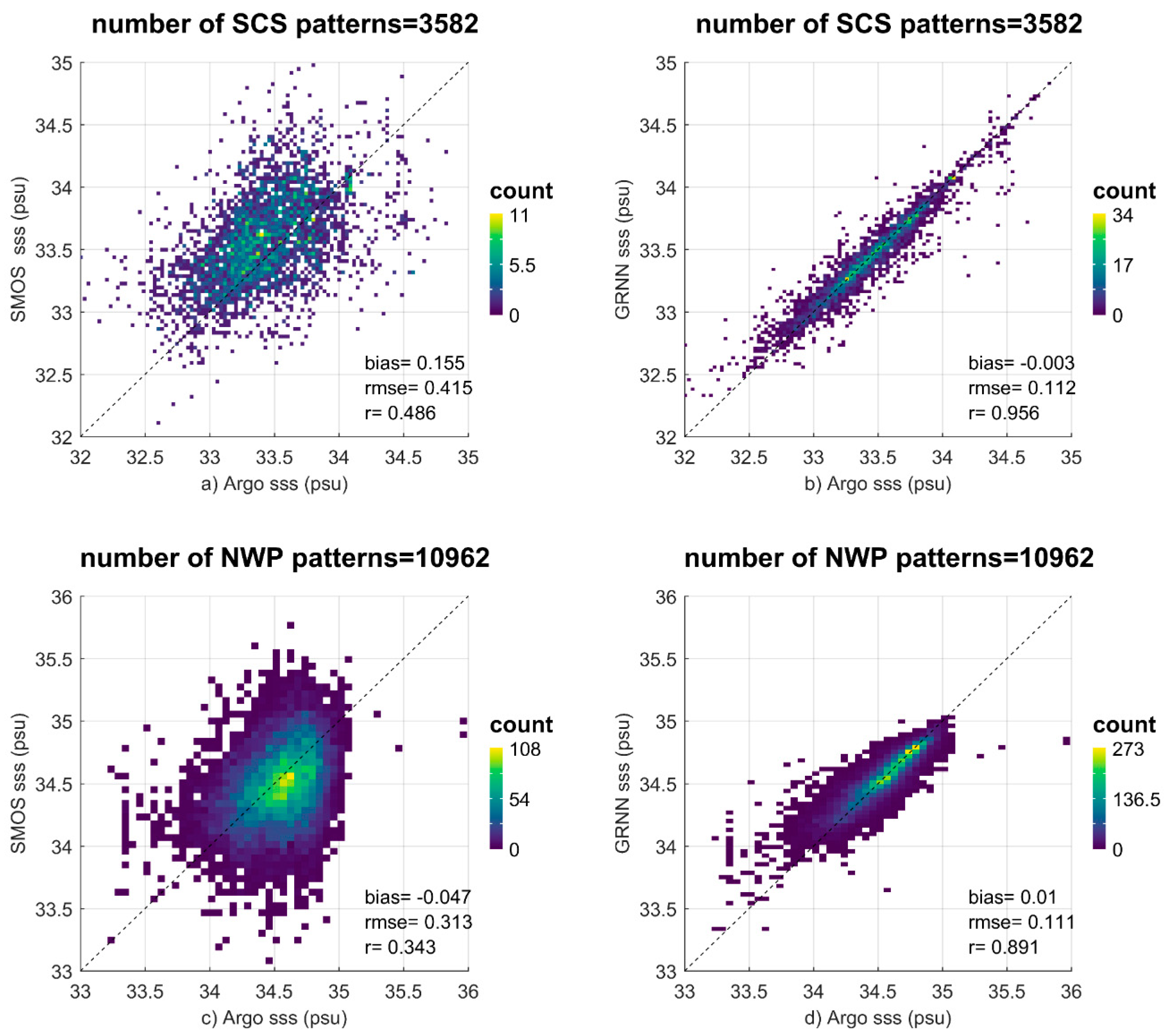
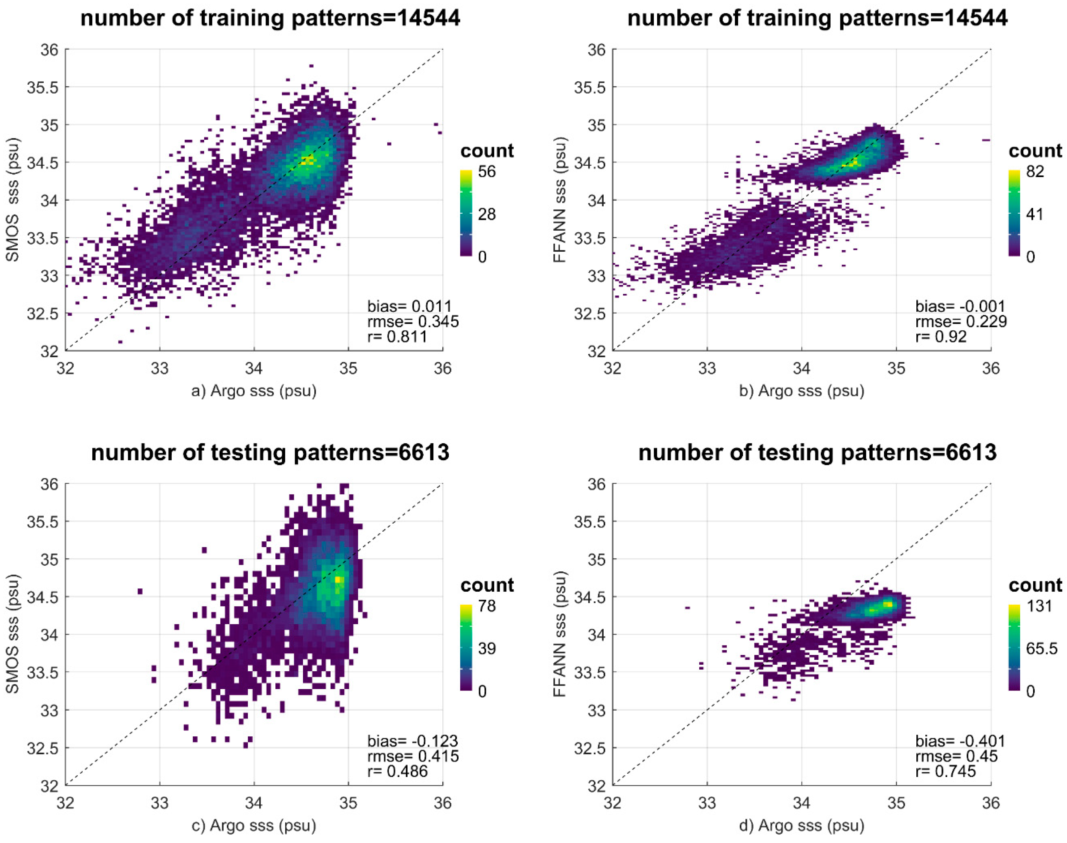
2.4. Analysis of the GRNN Correction Results

The corrected SSS are shown in Figure 3. In the figure, the corrected SSS are more consistent with the Argo float data both in SCS and northwestern Pacific. The bias and RMSE are significantly decreased. In the SCS (3582 observation points), the bias is reduced from 0.155 PSU (before correction) to −0.003 PSU (after correction), and the RMSE is reduced from 0.415 PSU (before correction) to 0.112 PSU (after correction). In the northwestern Pacific (10,962 observation points), the bias and RMSE are reduced from −0.047 PSU and 0.313 PSU to 0.01 PSU and 0.111 PSU, respectively. The corrected SMOS daily SSS are also compared with the ISAS-15 dataset (Figure 4). The topmost layer of ISAS-15 salinity locates at 1 m depth and the vertical salinity gradients in the top few meters are small [32], and the mean errors of ISAS SSS are approximately 0.1 PSU in SCS and 0.05 PSU in western Pacific according to the parameter of the ISAS-15 dataset; therefore, SMOS SSS and the ISAS-15 topmost layer salinity are comparable and the comparison is meaningful. Except in coastal regions where the depth is less than 200 m and there are no Argo floats observations, the bias and RMSE of the corrected SSS are significantly reduced in the SCS and the northwestern Pacific and the variability of the corrected SSS maintains the same order as SSS of the ISAS dataset (see Appendix A). Notably, the error in the Luzon Strait is very large even after the correction due to the lack of Argo float data (shown in Figure 5). Therefore, the subsequent assimilation experiments and analysis exclude the Luzon Strait and shallow water area where depth is less than 200 m). In general, the SSS error has been significantly reduced using the GRNN method; thus the corrected SSS can be used in the data assimilation system. The GRNN correction results are also better than FFANN correction results of Vernieres et al. [15] for these two areas (see Appendix B).

3. Assimilation of Corrected SSS in the Regional Ocean Modeling System (ROMS) 4DVAR System

3.1. The Regional Ocean Modeling System (ROMS) Ocean Model and 4DVAR

In this study, the dynamic model is the Regional Ocean Modeling System (ROMS). ROMS solves the hydrostatic primitive equations in horizontal curvilinear coordinates and vertical $\mathsf{\sigma }$ coordinates [33,34]. The model domain covers the northern SCS and northwestern Pacific (105°E-128°E, 15.5°N-24°N) with a horizontal resolution of 1/12° × 1/12° and 32 vertical $\mathsf{\sigma }$ levels. The assimilation time window is 7 days, and the total experimental duration is 2 years (01/01/2012 to 30/12/2013), containing105 assimilation windows.

The model was driven by the climatological forcing (COADS) for 20 years from the initial state extracted from the climatological Simple Ocean Data Assimilation (SODA) dataset, which is considered to be the model spin-up process. Then the model is integrated for the 2001–2015 period with the real forcing conditions (heat flux, freshwater flux, and wind stresses) and open boundary conditions (except the western boundary). The data used for the real simulation are summarized in

Table 1. Information of the forcing fields and boundary conditions datasets.

Variable	Horizontal Resolution	Temporal Resolution	Source
Heat flux	0.75° × 0.75°	6 h	ERA-interim [35]
Freshwater flux	0.75° × 0.75°	6 h	ERA-interim
Wind stresses	0.25° × 0.25°	6 h	${\mathrm{CCMP} }^1$ [36]
Boundary conditions	–	–	${\mathrm{SODA} }^2$ [37]

¹ The wind stresses are derived from CCMP version2.0 by a bulk formula; ² the SODA dataset used in this study is version3.3.1.

.

The 4-dimensional variational (4DVAR) assimilation system is based on incremental 4-dimensional variational assimilation (I4DVAR) [38,39]. I4DVAR seeks the optimal state of the ocean by adjusting the initial field, forcing field, and boundary conditions. The detailed theory is described in [40,41]. The observational measurements error is set with the standard deviation as follows [38]: 2cm for SSH, 0.4°C for SST, 0.1°C for in situ temperature(T), and 0.01 PSU for in situ salinity (S). The standard deviations of the raw SMOS SSS and corrected SSS are set to 0.4 PSU and 0.1 PSU, according to the RMSE in comparison with the Argo data (Figure 3).

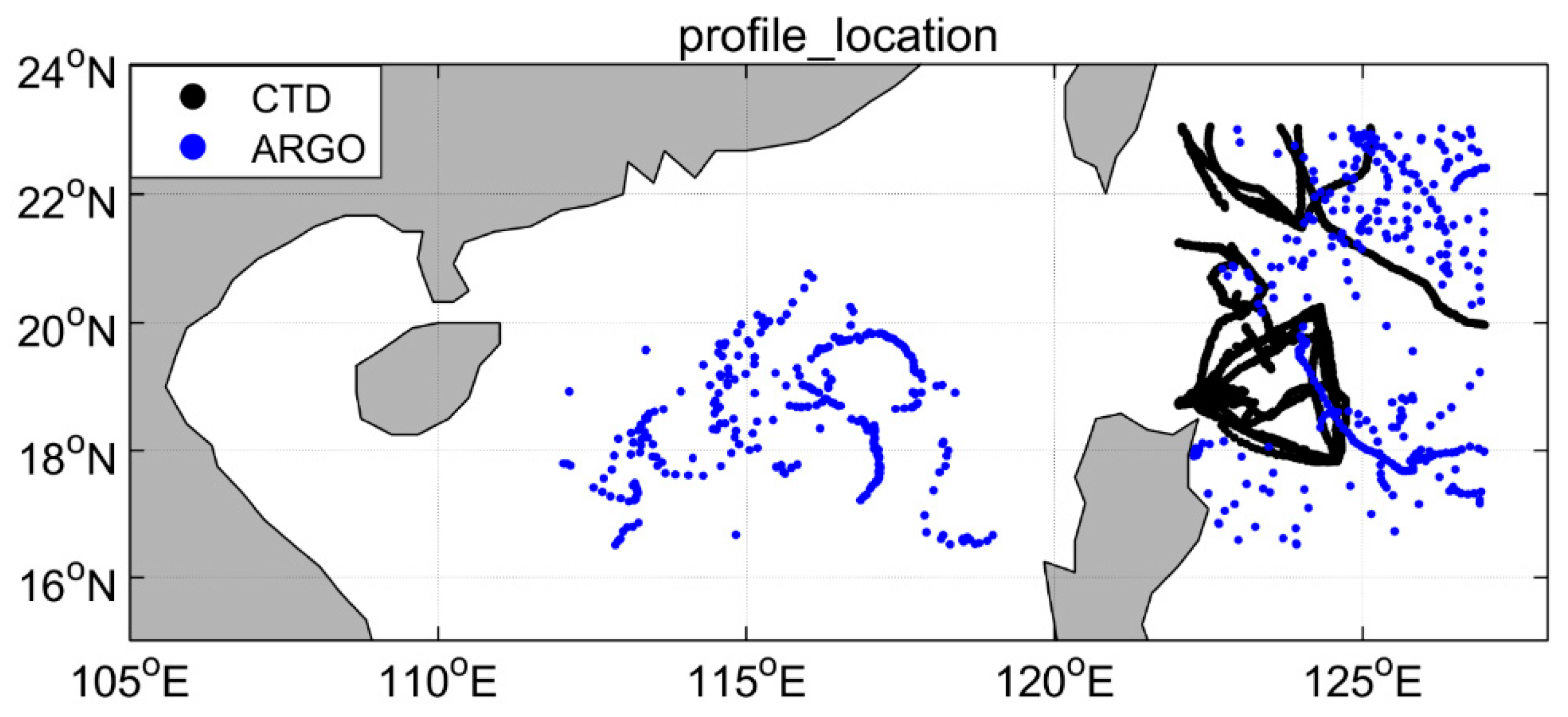
3.2. Data Used for the Assimilation

The following data sets are used in the assimilation: (1) SMOS BEC L3 objective analysis data set; (2) NOAA optimal interpolation SST; (3) Aviso’s SLA data; and (4) the Met Office Hadley Centre EN4 data set of global quality-controlled ocean temperature and salinity profiles from the European Union ENSEMBLES project (EN4) [42]. Before assimilation into the model, the temperature and salinity profile data were interpolated to the standard 23 z-levels: (−5 m, −10 m, −15 m, −20 m, −25 m, −30 m, −35 m, −40 m, −50 m, −60 m, −75 m, −100 m, −125 m, −150 m, −200 m, −250 m, −300 m, −400 m, −500 m, −600 m, −800 m, −1000 m, and −1200 m) with the cubic spline interpolation method.

Data for verification include the following: (1) ISAS-15 gridded salinity data; (2) northern SCS sailing ship T/S data published by the National Earth System Science Data Sharing Infrastructure, National Science & Technology Infrastructure of China (http://www.geodata.cn); the dataset comprises CTD observations along 18°N from 111.5°E to 118°E during the period of 12/08/2012 to 21/08/2012 in SCS; and (3) the interpolated EN4 profile data are also used for verification.

3.3. Experimental Setup

Six experiments were designed to evaluate the impact of GRNN preprocessing on SSS assimilation and the impact of SSS assimilation on surface and subsurface salinity simulations. Experiment 1 (EX1) did not assimilate any data and is referred to as the control experiment (BASE). EX2 (RAW) and EX3 (NN) assimilated the raw and corrected SSS, respectively. EX4 (OTH) assimilated other observations (SST, SLA, and T/S profile) except the SSS. EX5 (RAWALL) and EX6 (NNALL) add the raw and corrected SSS, respectively to the EX4 dataset. The experimental summary is shown in

Table 2. Summary of the experiments.

Experiments	Experiments Name	Data Assimilated
EX1	BASE	None
EX2	RAW	Raw SMOS SSS
EX3	NN	Corrected SMOS SSS
EX4	OTH	SSH, SST, T/S profile
EX5	RAWALL	Raw SMOS SSS, SSH, SST, T/S profile
EX6	NNALL	Corrected SMOS SSS, SSH, SST, T/S profile

.

4. Assimilation Results

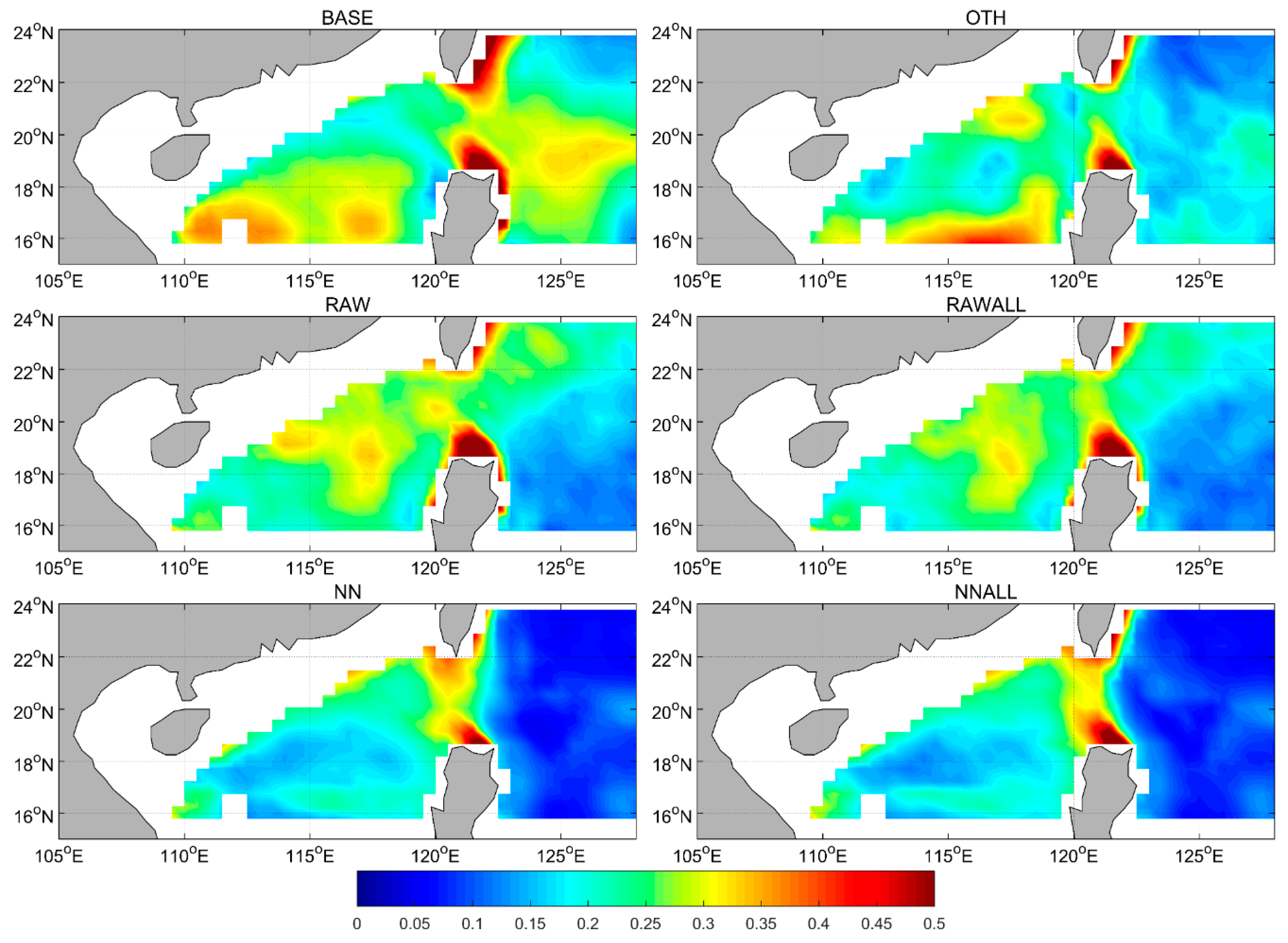
In this paper, to evaluate the impact of SSS assimilation on surface and subsurface salinity, the experimental results were compared with the surface and subsurface salinity of ISAS-15, the salinity profiles of the EN4 dataset, and the SCS shipboard data. The 18°N section is the trans-sea basin section in the northernmost part of the SCS. The section is adjacent to the Luzon Strait. The water masses were being exchanged between the North Pacific and SCS or the circulation inside the SCS both pass through this section [43,44]; therefore, we wanted to know how the assimilation of satellite SSS affected the salinity profile in this section.

4.1. SSS Analysis

We evaluated the assimilation effect by comparing the model SSS residual with the ISAS-15 SSS for the period of 2012–2013, the results are shown in Figure 6. There were large SSS errors in the BASE experiment (~0.3 PSU in the research region), which were expected because no data were assimilated in the BASE experiment. The raw SSS assimilation led to a slight improvement over the BASE experiment due to the large error in raw SSS (EX2). However, the SSS errors are less than 0.1 PSU in the northwestern Pacific and 0.15 PSU in the northern SCS after the SSS is corrected and assimilated into the model, (EX3, Figure 6, NN), which is also verified in the NNALL experiment (EX6), indicating that the assimilation of the corrected SSS can improve the model SSS simulation.

Although the EX4 did not directly assimilate the SSS observations, there are still some improvements in the northwestern Pacific, which is consistent with the previous study [16], but large errors exist in the northern SCS, which changed slightly compared with the control experiment. Comparing EX4 and EX5, the raw SSS assimilation would also slightly reduce the performance of traditional observations (SSH, SST, and T/S profile), while the corrected SSS can further improve the SSS simulation based on EX4 (see Figure 6, NNALL). Generally, the GRNN method significantly reduced the error in the raw SSS and yielded a positive impact on the SSS assimilation.

4.2. Subsurface Salinity Analysis

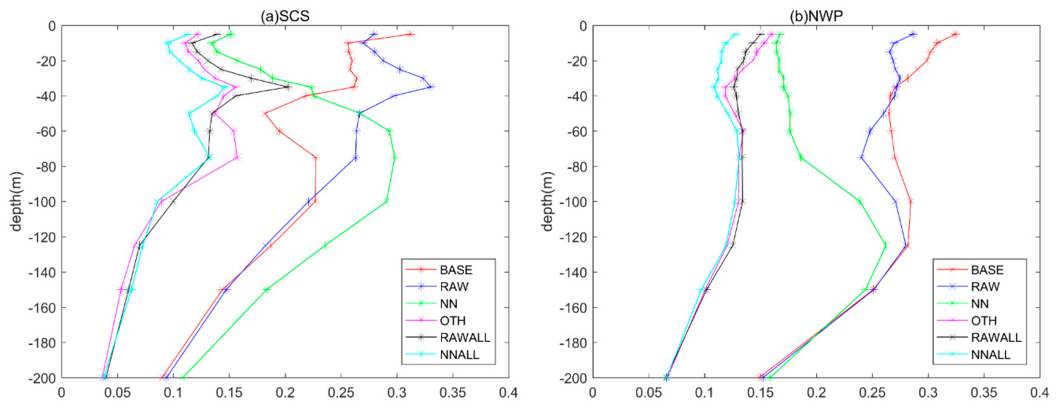
4.2.1. Salinity Profile

The SSS corrections are likely to propagate vertically through the background error covariance and model dynamics, and SSS assimilation can impact subsurface salinity simulations, which has been demonstrated on a global scale by Lu et al. and G. Vernieres et al. [15,16]. Whether the SSS preprocessed through GRNN yields a positive impact on the subsurface layer in northern SCS needs to be verified, and the question of SSS influence depth is also of concern. The subsurface SSS are compared with the EN4 dataset, as shown in Figure 7 (the locations of observation are shown in Figure 8). The raw SSS data assimilation deteriorated the subsurface salinity field to a depth of 100 m. The corrected SSS assimilation improved the subsurface salinity field compared with the BASE experiment, except in the thermocline [45]. However, the thermocline errors can be reduced by assimilation of T/S profiles, such as in OTH and NNALL experiments. The influence depths of the corrected SSS are different in the northern SCS and northwestern Pacific. Compared with the BASE experiment, the corrected SSS yields a positive impact at the 150 m depth in the northwestern Pacific but is only positive at 40 m in the northern SCS. One reason is the difference in seawater properties between the SCS and the northwestern Pacific [46].

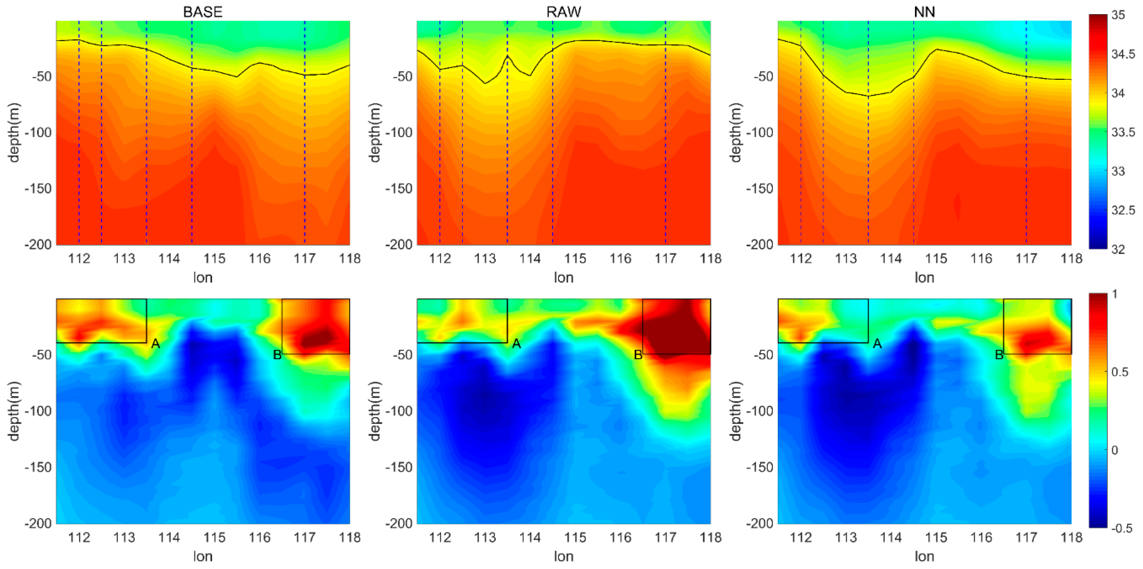
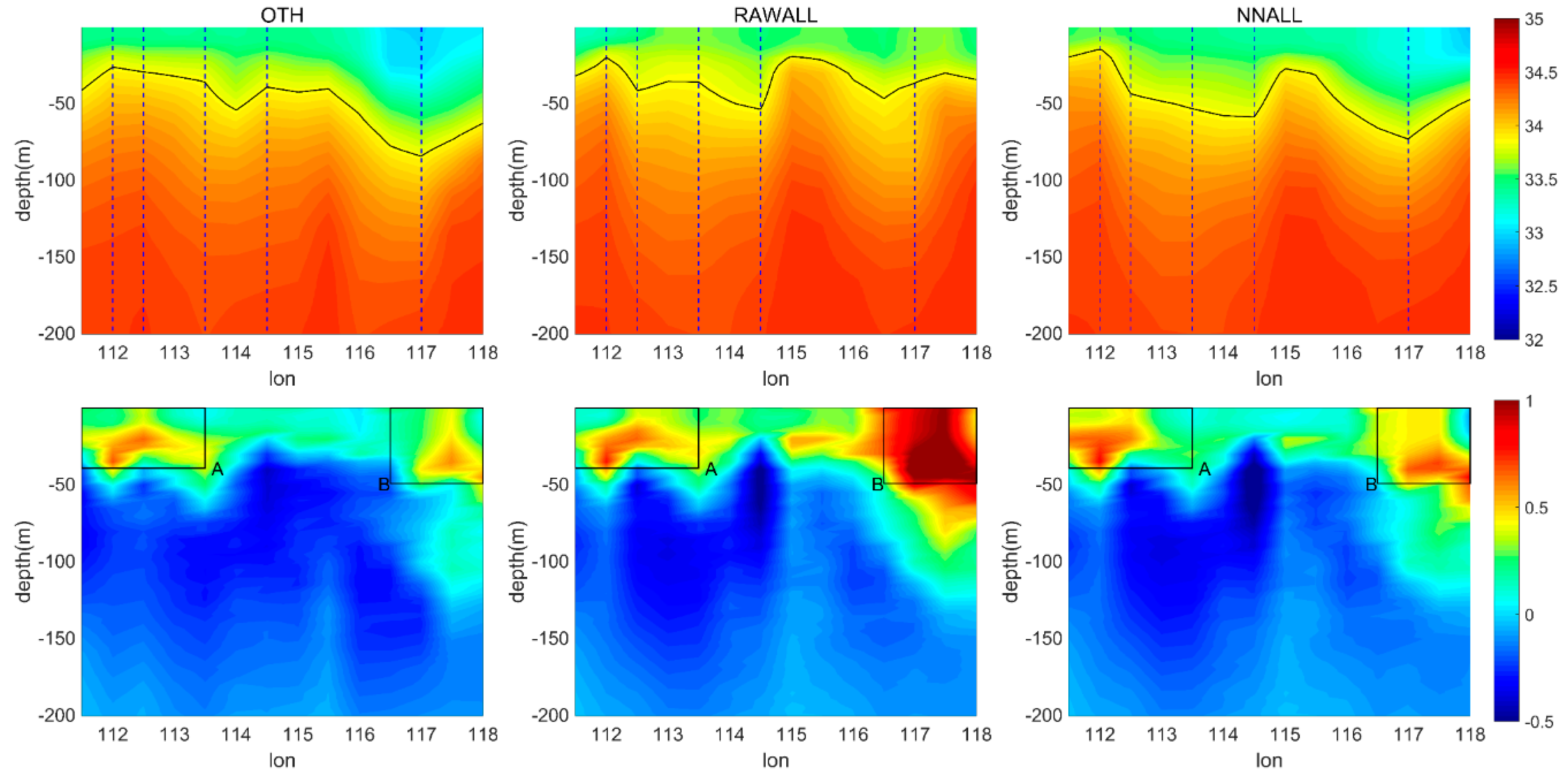
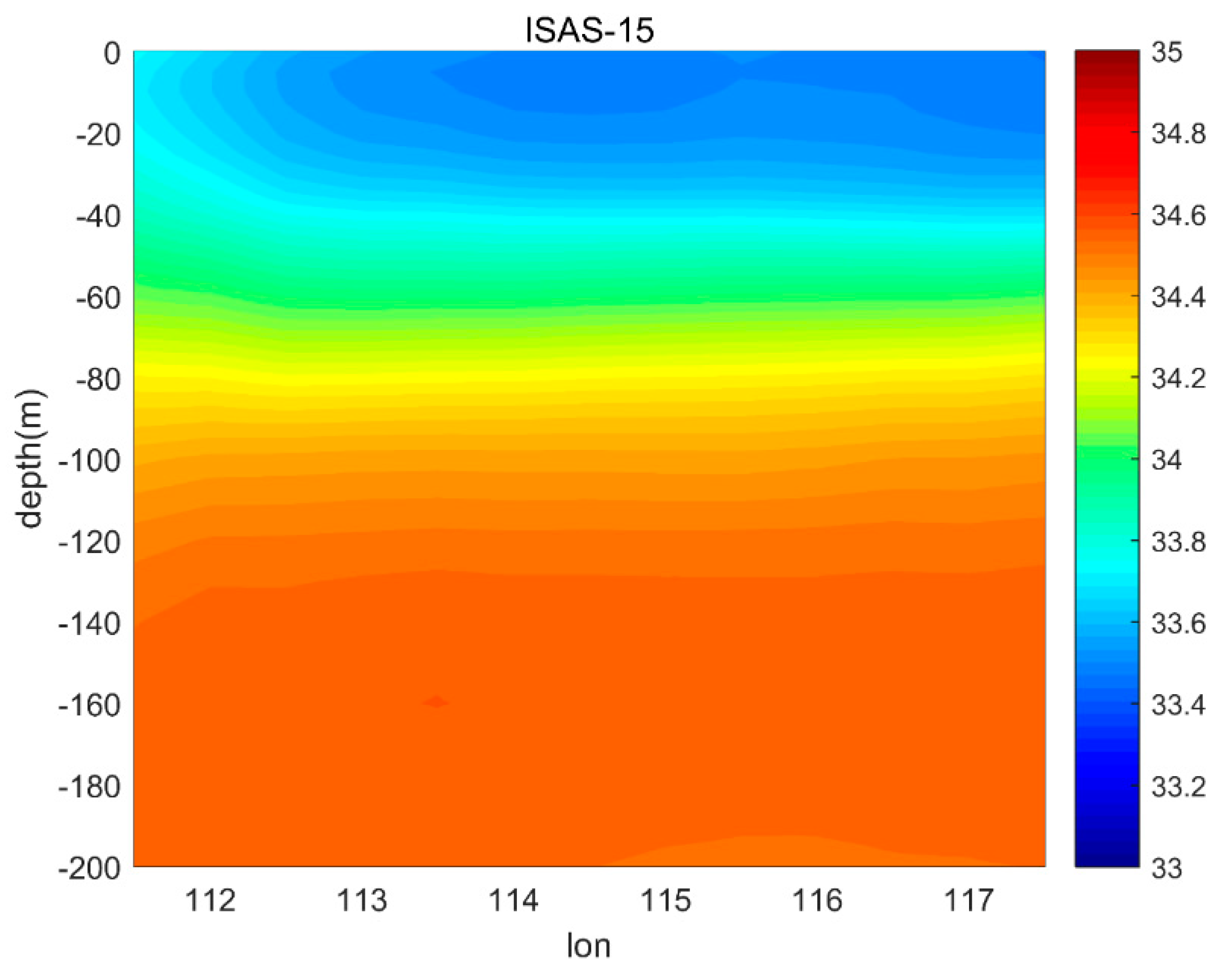
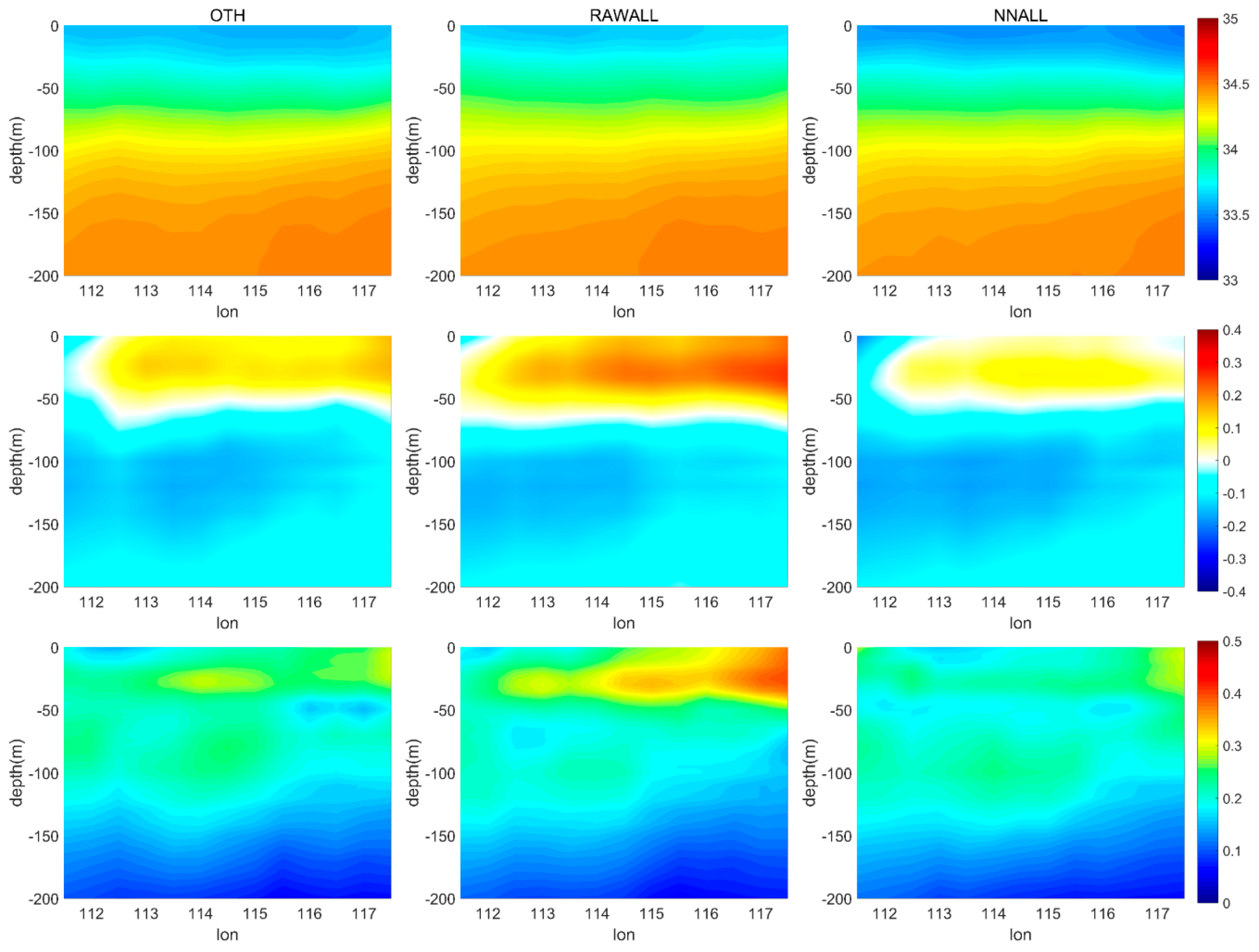
4.2.2. Salinity Section

To be more objective, the impact of SSS assimilation on the subsurface salinity is verified with the CTD observations from the northern SCS sailing data that have not been used in the GRNN and the assimilation. Additional experiments were carried out during the 12/08/2012–21/08-2013 period for consistency with the CTD observational period. The observational map is shown in Figure 9.

The results of the first three experiments’ differences from the sailing data are shown in Figure 10. The biases are calculated by subtracting observations from model results. The simulation results of the model background SSS field are saltier than the SSS of CTD observations in areas A and B, and is fresher overall below 50 m. The raw SSS assimilation reduces the error in area A but introduces larger errors in area B, that is because the raw SSS is saltier than the sailing data. The corrected SSS assimilation significantly reduces the error in areas A and B. However, a new error is introduced at depths of 50–120 m compared with the BASE result. This finding shows that the assimilation of SSS corrected by GRNN has a positive impact on the salinity in the mixed layer, but a negative impact in the thermocline, which is consistent with the results shown in Figure 7.

Figure 11 shows the salinity section of the assimilation results for EX4, EX5, and EX6, and their biases compared with the observations. The assimilation of traditional observations in the OTH experiment improves the subsurface salinity field, reducing the deviation to less than 0.5 PSU in areas A and B. The assimilation of the traditional observations and raw SSS (EX5) yields a slight improvement in area B compared with the RAW experiment, but the bias in area B is still larger than the control run BASE due to high differences between the raw SSS and sailing data. Raw SSS assimilation dominates on this section and the effect of traditional observations assimilation does not show up clearly. Assimilating traditional observations and corrected SSS significantly improves the simulation of areas A and B compared with BASE and RAWALL results, and the salinity adjustment on this section mainly depends on traditional observations assimilation by comparing NN, OTH, and NNALL results. However, the impact of SSS assimilation on this salinity section simulation changes from negative one to positive one after GRNN correction.

Notably, there are actually no T/S profiles data assimilated along 18°N during 12/08/2012–21/08/2013. The improvements in EX4 (Figure 11, OTH) are mainly contributed by the SST and SLA. To further demonstrate the SSS assimilation influence on the subsurface salinity field, the experimental results were compared with the ISAS-15 dataset along 18°N for the period of 2012–2013, as shown in Figure 12, Figure 13 and Figure 14. The mean biases are obtained by calculating the mean difference (subtracting ISAS-15 section salinity values from monthly mean model simulations). The salinity section of BASE in the mixed layer is saltier (+0.3 PSU), while the salinity in and below the thermocline is fresher (−0.2 PSU) and the area with the highest error is the eastern section above −50 m according to the RMSE of BASE simulations compared with the ISAS-15 dataset. The raw SSS assimilation slightly improves the western mixed layer salinity field on the section, but introduces large errors in the eastern part of the mixed layer. The corrected SSS can significantly improve the salinity simulation effect of the mixed layer compared with BASE and RAW experiments. However, the salinity simulation effect is slightly reduced below 60 m and the RMSE is still approximately 0.3 PSU in the eastern mixed layer. The EX6 results show that the long-term assimilation of traditional observations can help reduce the RMSE and improve the salinity fields simulation based on the corrected SSS assimilation. A comparison of EX3, EX4, and EX6 shows that the improvement in the mixed layer salinity simulation effect mainly originates from the SSS assimilation. Assimilation of traditional observations can obtain a similar effect, and the NN simulation results are even better in most areas of the mixed layer.

5. Discussion

The SMOS satellite has provided long-term, high-resolution, large-scale SSS data since operation of the satellite began, which has played a significant role in simulation of the ocean state; however, SSS retrieval is difficult in the coastal ocean, high latitudes, and other regions affected by RFI, especially in Asia, where the data accuracy is too low to be used in assimilations. Therefore, it is necessary to implement preprocessing when using satellite salinity data in these regions (such as the SCS). In this paper, we introduce the GRNN to correct satellite salinity and significantly improve the accuracy to assimilate SSS and provide a better estimate of the state of the ocean. The main components of the GRNN input vector are longitude, latitude, observation time, SST, SLA, and SMOS SSS in this study. If necessary, new variables can be added into the input vector after taking into account other factors that may induce errors in the SSS retrieval process, but which may also induce new errors if the new variables deteriorate the previous joint distribution.

Thus far, our work has made progress on SMOS SSS assimilations in the coastal ocean, but there are still some problems to be solved and work that must be continued in the future. (1) Taking the topmost Argo observations as truth may introduce new errors in the regions where vertical stratification is strong [15,47]. The satellites measure the SSS in the ocean skin layer, approximately 1 cm, whereas the Argo measurements locate at approximately 5–10 m depth. The evaporation-induced and precipitation-induced salinity anomalies are neglected in this study, but heavy precipitation would cause the SSS to change for several hours and introduce strong stratification in the top few meters [18,48] and there would be large biases between Argo measurements and true SSS (~1 cm); the Argo data cannot be used as “truth” anymore. Except that, the Argo measurements are single point observations and SSS of satellite product is an average of a pixel. Although the spatial variability of SSS in a pixel is low, there are still differences between satellite observations and Argo measurements. The GRNN has poor performance on SSS correction in the Luzon Strait has two reasons, one is the GRNN model problem: (i) SSS have high variability in the Luzon Strait because of Kuroshio invasion and the Argo measurements are sparse in this region and cannot capture the feature. (ii) The information of SSS spatial and temporal variability is not transferred into the model, supporting with the consistency between the patterns of RMSE of corrected SSS compared with ISAS15 and the locations of Argo observations. (iii) There are large errors in the areas with less Argo measurements and smaller errors in the areas with more Argo observations (Figure 4d and Figure 5). The other is the validation dataset problem—the errors of the validation set ISAS15 are large in Luzon Strait (as shown in Figure 15), leading to the large RMSE between corrected SSS and ISAS surface salinity. (2) SMOS SSS corrections should be obtained at a global scale, especially in high latitude regions. The satellite SSS measurements have lower accuracy at high latitudes due to the reduced signal-to-noise ratio in colder waters [20]. These low temperature-induced errors may can also be corrected by NNs, and this topic deserves future study. (3) Corrected SSS should be obtained in areas with depth shallower than 200 m and where there are few Argo floats (the Luzon Strait) by utilizing the analysis field obtained by assimilating corrected SSS to correct satellite SSS. By assimilating the corrected SSS in the region where depths are greater than 200 m, the SSS in the shallow region can also be adjusted. Sampling from the assimilation analysis field and taking the sample dataset as “truth,” SSS in the shallow regions may have a higher accuracy after correction. Therefore, future work will focus on the above three aspects to obtain more accurate satellite salinity data and better estimates of the ocean state.

6. Conclusions

In this paper, the objective analysis data set of SMOS SSS has been corrected by GRNN in SCS and northwestern Pacific and applied to the assimilation system. To verify the effect of SSS assimilation in coastal regions, six experiments were designed and the assimilation results were compared with the ISAS15 dataset and the sailing dataset. The conclusions are as follows:

(a)

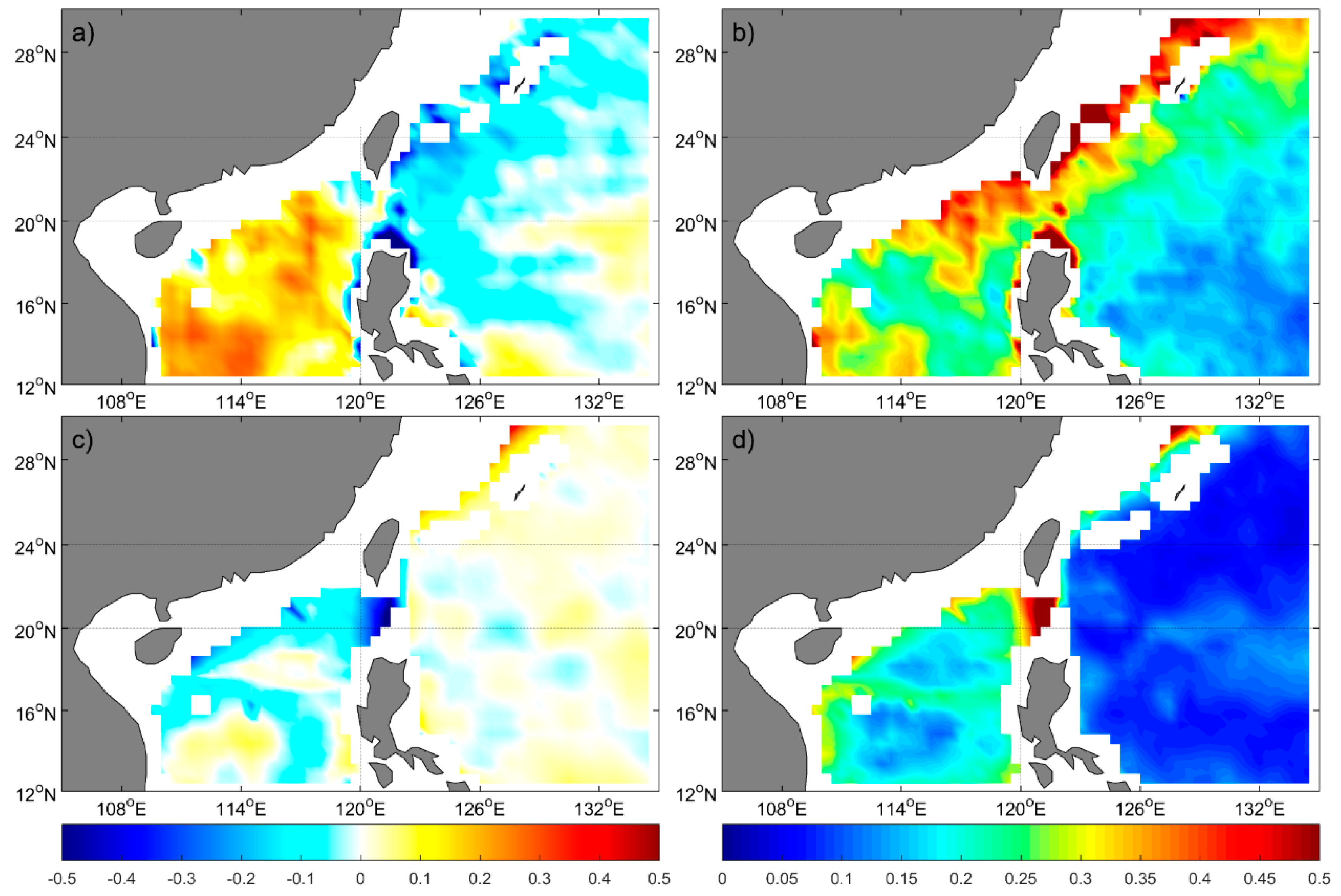
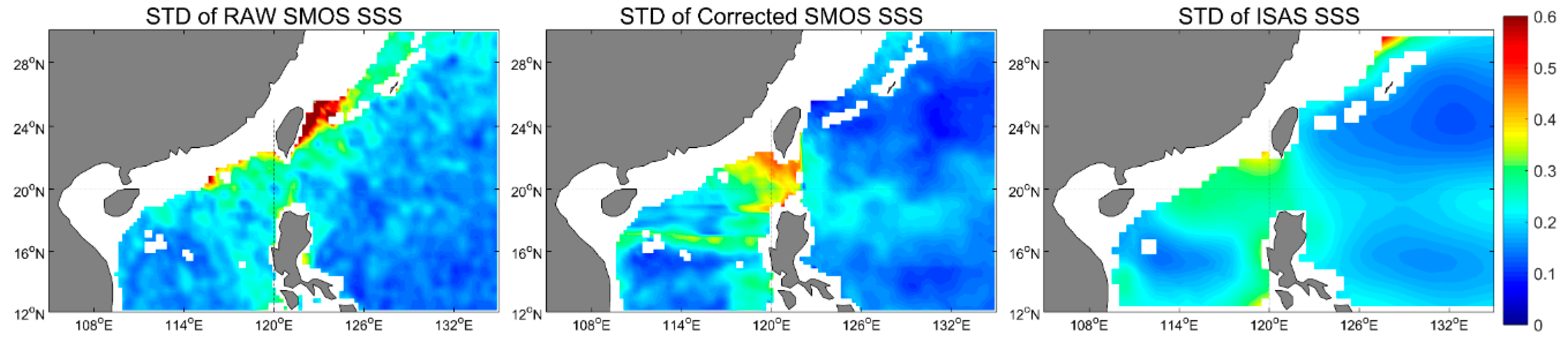
Compared with Argo floats data, in addition to the northwestern Pacific, the errors in SSS product have also been reduced significantly in the northern SCS after being corrected by GRNN. The bias and RMSE are reduced to the order of 0.01 PSU and 0.1 PSU. The mean bias and RMSE compared with ISAS-15 SSS for the period of 2012–2014 are reduced and the variability of the corrected SSS maintains the same order as SSS of the ISAS dataset.

(b)

T/S profiles assimilation can yield a positive impact on northwestern Pacific SSS simulations, but only slightly influences northern SCS SSS, while the assimilation of both raw SSS and GRNN corrected SSS yields improvements on model SSS. The largest improvements are shown in experiments with GRNN corrected SSS assimilation (EX3 and EX6), proving the importance of GRNN for SSS correction.

(c)

Comparing the experimental results with EN4 profiles shows that the assimilation of corrected SSS also improved the salinity fields simulation in the mixed layer, except for horizontal improvements on sea surface. Below the mixed layer, T/S profiles data are more important than SSS data. The influence depths of SSS assimilation are shallower in the northern SCS than in the northwestern Pacific, which indicates that the corrected SSS should be assimilated with T/S profiles data to obtain a better estimation of ocean states in coastal regions. However, after long-term assimilation, the improvements generated by corrected SSS assimilation are better than those from traditional observations’ assimilations in most areas of the 18°N section in the SCS.

References

1. Derber, J.; Rosati, A. A global oceanic data assimilation system. J. Phys. Oceanogr. 1989, 19, 1333–1347. [Google Scholar] [CrossRef]
2. Clancy, R.M.; Phoebus, P.A.; Pollak, K.D. An operational global-scale ocean thermal analysis system. J. Atmos. Ocean. Technol. 1990, 7, 233–254. [Google Scholar] [CrossRef]
3. Meyers, G.; Phillips, H.; Smith, N.; Sprintall, J. Space and time scales for optimal interpolation of temperature—Tropical Pacific Ocean. Prog. Oceanogr. 1991, 28, 189–218. [Google Scholar] [CrossRef]
4. Shu, Y.; Zhu, J.; Wang, D.; Yan, C.; Xiao, X. Performance of four sea surface temperature assimilation schemes in the South China Sea. Cont. Shelf Res. 2009, 29, 1489–1501. [Google Scholar] [CrossRef] [Green Version]
5. Cooper, N.S. The effect of salinity on tropical ocean models. J. Phys. Oceanogr. 1988, 18, 697–707. [Google Scholar] [CrossRef]
6. Murtugudde, R.; Busalacchi, A.J. Salinity effects in a tropical ocean model. J. Geophys. Res. Oceans 1998, 103, 3283–3300. [Google Scholar] [CrossRef] [Green Version]
7. Roemmich, D.; Gilson, J. The 2004–2008 mean and annual cycle of temperature, salinity, and steric height in the global ocean from the Argo Program. Prog. Oceanogr. 2009, 82, 81–100. [Google Scholar] [CrossRef]
8. Han, G.; Zhu, J.; Zhou, G. Salinity estimation using the T-S relation in the context of variational data assimilation. J. Geophys. Res. Oceans 2004, 109, C03018. [Google Scholar] [CrossRef]
9. Zhu, J.; Zhou, G.; Yan, C.; Fu, W.; You, X. A three-dimensional variational ocean data assimilation system: Scheme and preliminary results. Sci. China Ser. D Earth Sci. 2006, 49, 1212–1222. [Google Scholar] [CrossRef]
10. Durack, P.J.; Wijffels, S.E. Fifty-year trends in global ocean salinities and their relationship to broad-scale warming. J. Clim. 2010, 23, 4342–4362. [Google Scholar] [CrossRef]
11. Freeland, H.; Roemmich, D.; Garzoli, S.; Le Traon, P.Y.; Ravichandran, M.; Riser, S.; Thierry, V.; Wijffels, S.; Belbéoch, M.; Gould, J. Argo-a decade of progress. In Proceedings of the OceanObs’ 09: Sustained Ocean Observations and Information for Society, Venice, Italy, 21–25 September 2009; Volume 2. [Google Scholar]
12. Hackert, E.; Ballabrera-Poy, J.; Busalacchi, A.J.; Zhang, R.H.; Murtugudde, R. Impact of sea surface salinity assimilation on coupled forecasts in the tropical Pacific. J. Geophys. Res. Oceans 2011, 116, C05009. [Google Scholar] [CrossRef]
13. Hackert, E.; Busalacchi, A.J.; Ballabrera-Poy, J. Impact of Aquarius sea surface salinity observations on coupled forecasts for the tropical Indo-Pacific Ocean. J. Geophys. Res. Oceans 2014, 119, 4045–4067. [Google Scholar] [CrossRef] [Green Version]
14. Chakraborty, A.; Sharma, R.; Kumar, R.; Basu, S. A SEEK filter assimilation of sea surface salinity from Aquarius in an OGCM: Implication for surface dynamics and thermohaline structure. J. Geophys. Res. Oceans 2014, 119, 4777–4796. [Google Scholar] [CrossRef] [Green Version]
15. Vernieres, G.; Kovach, R.; Keppenne, C.; Akella, S.; Brucker, L.; Dinnat, E. The impact of the assimilation of Aquarius sea surface salinity data in the GEOS ocean data assimilation system. J. Geophys. Res. Oceans 2014, 119, 6974–6987. [Google Scholar] [CrossRef] [Green Version]
16. Lu, Z.; Cheng, L.; Zhu, J.; Lin, R. The complementary role of SMOS sea surface salinity observation for estimating global ocean salinity state. J. Geophys. Res. Oceans 2016, 121, 3672–3691. [Google Scholar] [CrossRef]
17. Köhl, A.; Sena Martins, M.; Stammer, D. Impact of assimilating surface salinity from SMOS on ocean circulation estimates. J. Geophys. Res. Oceans 2014, 119, 5449–5464. [Google Scholar] [CrossRef] [Green Version]
18. Kerr, Y.H.; Waldteufel, P.; Wigneron, J.P.; Delwart, S.; Cabot, F.; Boutin, J.; Escorihuela, M.-J.; Font, J.; Reul, N.; Gruhier, C.; et al. The SMOS mission: New tool for monitoring key elements ofthe global water cycle. Proc. IEEE 2010, 98, 666–687. [Google Scholar] [CrossRef]
19. Boutin, J.; Martin, N.; Yin, X.; Font, J.; Reul, N.; Spurgeon, P. First assessment of SMOS data over open ocean: Part II, sea surface alinity. IEEE Trans. Geosci. Remote Sens. 2012, 50, 1662–1675. [Google Scholar] [CrossRef]
20. Vinogradova, N.T.; Ponte, R.M.; Fukumori, I.; Wang, O. Estimating satellite salinity errors for assimilation of Aquarius and SMOS data into climate models. J. Geophys. Res. Oceans 2014, 119, 4732–4744. [Google Scholar] [CrossRef] [Green Version]
21. Zhang, H.; Chen, G.; Qian, C.; Jiang, H. Assessment of two SMOS sea surface salinity level 3 products against Argo upper salinity measurements. IEEE Geosci. Remote Sens. Lett. 2013, 10, 1434–1438. [Google Scholar] [CrossRef]
22. Olmedo, E.; Martínez, J.; Turiel, A.; Ballabrera-Poy, J.; Portabella, M. Debiased non-Bayesian retrieval: A novel approach to SMOS Sea Surface Salinity. Remote Sens. Environ. 2017, 193, 103–126. [Google Scholar] [CrossRef]
23. Ammar, A.; Labroue, S.; Obligis, E.; Mejia, C.; Thiria, S.; Crepon, M. Sea surface salinity retrieval throughout a SMOS half-orbit using neural networks. In Proceedings of the 2006 IEEE MicroRad, SanJuan, Puerto Rico, 28 February–3 March 2006; pp. 103–108. [Google Scholar]
24. Gao, S.; Tian, J.; Wang, F.; Bai, Y.; Gao, W.; Yang, S. The study of GRNN for wind speed forecasting based on Markov Chain. In Proceedings of the International Conference on Modelling, Simulation and Applied Mathematics (MSAM 2015), Phuket, Thailand, 23–24 August 2015; pp. 285–288. [Google Scholar]
25. Zhou, K.; Yu, D.; Lin, Z.; Cao, B.; Wang, Z.; Guo, S. Anode effect prediction of aluminum electrolysis using GRNN. In Proceedings of the 2015 Chinese Automation Congress (CAC), Wuhan, China, 27–29 November 2015; pp. 853–858. [Google Scholar]
26. Carval, T.; Keeley, B.; Takatsuki, Y.; Yoshida, T.; Loch, S.; Schmid, C.; Goldsmith, R.; Wong, A.; McCreadie, R.; Thresher, A.; et al. ARGO Data Management: 2012. Argo User’s Manual v2.4. IFREMER Reference cor-do/dti-mut/02-084. Available online: http://www.argodatamgt.org/content/download/12096/80327/file/argo-dm-user-manual.pdf (accessed on 9 September 2014).
27. Reynolds, R.W.; Smith, T.M.; Liu, C.; Chelton, D.B.; Casey, K.S.; Schlax, M.G. Daily high-resolution-blended analyses for sea surface temperature. J. Clim. 2007, 20, 5473–5496. [Google Scholar] [CrossRef]
28. Nicolas, K.; Annaig, P.; Fabienne, G. ISAS-SSS: In Situ Sea Surface Salinity Gridded Fields. SEANOE: 2018. Available online: https://doi.org/10.17882/55600 (accessed on 1 June 2018).
29. Gaillard, F.; Reynaud, T.; Thierry, V.; Kolodziejczyk, N.; von Schuckmann, K. In-situ based reanalysis of the global ocean temperature and salinity with ISAS: Variability of the heat content and steric height. J. Clim. 2016, 29, 1305–1323. [Google Scholar] [CrossRef]
30. Bao, S.; Zhang, R.; Wang, H.; Yan, H.; Yu, Y.; Chen, J. Salinity Profile Estimation in the Pacific Ocean from Satellite Surface Salinity Observations. J. Atmos. Ocean. Technol. 2019, 36, 53–68. [Google Scholar] [CrossRef]
31. Boutin, J.; Waldteufel, P.; Martin, N.; Caudal, G.; Dinnat, E. Surface salinity retrieved from SMOS measurements over the global ocean: Imprecisions due to sea surface roughness and temperature uncertainties. J. Atmos. Ocean. Technol. 2004, 21, 1432–1447. [Google Scholar] [CrossRef]
32. Anderson, J.E.; Riser, S.C. Near-surface variability of temperature and salinity in the near-tropical ocean: Observations from profiling floats. J. Geophys. Res. Oceans 2014, 119, 7433–7448. [Google Scholar] [CrossRef] [Green Version]
33. Shchepetkin, A.F.; McWilliams, J.C. A method for computing horizontal pressure-gradient force in an oceanic model with a nonaligned vertical coordinate. J. Geophys. Res. 2003, 108. [Google Scholar] [CrossRef] [Green Version]
34. Shchepetkin, A.F.; McWilliams, J.C. The Regional Ocean Modeling System: A split-explicit, free-surface, topography following coordinates ocean model. Ocean Model. 2005, 9, 347–404. [Google Scholar] [CrossRef]
35. Dee, D.P.; Uppala, S.M.; Simmons, A.J.; Berrisford, P.; Poli, P.; Kobayashi, S.; Andrae, U.; Balmaseda, M.A.; Balsamo, G.; Bauer, P.; et al. The ERA-Interim reanalysis: Configuration and performance of the data assimilation system. Q. J. R. Meteorol. Soc. 2011, 137, 553–597. [Google Scholar] [CrossRef]
36. Atlas, R.; Hoffman, R.N.; Ardizzone, J.; Leidner, S.M.; Jusem, J.C.; Smith, D.K.; Gombos, D. A cross-calibrated, multiplatform ocean surface wind velocity product for meteorological and oceanographic applications. Bull. Am. Meteorol. Soc. 2011, 92, 157–174. [Google Scholar] [CrossRef]
37. Carton, J.A.; Chepurin, G.A.; Chen, L. SODA3: A new ocean climate reanalysis. J. Clim. 2018, 31, 6967–6983. [Google Scholar] [CrossRef]
38. Moore, A.M.; Arango, H.G.; Broquet, G.; Powell, B.S.; Weaver, A.T.; Zavala-Garay, J. The Regional Ocean Modeling System (ROMS) 4-dimensional variational data assimilation systems: Part I–System overview and formulation. Prog. Oceanogr. 2011, 91, 34–49. [Google Scholar] [CrossRef]
39. Moore, A.M.; Arango, H.G.; Broquet, G.; Edwards, C.; Veneziani, M.; Powell, B.; Foley, D.; Doyle, J.D.; Costa, D.; Robinson, P.; et al. The Regional Ocean Modeling System (ROMS) 4-dimensional variational data assimilation systems: Part II–performance and application to the California Current System. Prog. Oceanogr. 2011, 91, 50–73. [Google Scholar] [CrossRef]
40. Courtier, P.; Thépaut, J.N.; Hollingsworth, A. A strategy for operational implementation of 4D-Var, using an incremental approach. Q. J. R. Meteorol. Soc. 1994, 120, 1367–1387. [Google Scholar] [CrossRef]
41. Weaver, A.T.; Vialard, J.; Anderson, D.L.T. Three-and four-dimensional variational assimilation with a general circulation model of the tropical Pacific Ocean. Part I: Formulation, internal diagnostics, and consistency checks. Mon. Weather Rev. 2003, 131, 1360–1378. [Google Scholar] [CrossRef]
42. Good, S.A.; Martin, M.J.; Rayner, N.A. EN4: Quality controlled ocean temperature and salinity profiles and monthly objective analyses with uncertainty estimates. J. Geophys. Res. Oceans 2013, 118, 6704–6716. [Google Scholar] [CrossRef] [Green Version]
43. You, Y.; Chern, C.S.; Yang, Y.; Liu, C.T.; Liu, K.K.; Pai, S.C. The South China Sea, a cul-de-sac of North Pacific intermediate water. J. Oceanogr. 2005, 61, 509–527. [Google Scholar] [CrossRef]
44. Qu, T.; Mitsudera, H.; Yamagata, T. Intrusion of the north Pacific waters into the South China Sea. J. Geophys. Res. Oceans 2000, 105, 6415–6424. [Google Scholar] [CrossRef]
45. Liu, Q.; Jia, Y.; Liu, P.; Wang, Q.; Chu, P.C. Seasonal and intra-seasonal thermocline variability in the central South China Sea. Geophys. Res. Lett. 2001, 28, 4467–4470. [Google Scholar] [CrossRef]
46. Zeng, X. A Reanalysis Dataset of the South China Sea and Its Application in the Study of Mesoscale Eddies; South China Sea Institute of Oceanology Chinese Academy of Science: Guangzhou, China, 2015. [Google Scholar]
47. Henocq, C.; Boutin, J.; Reverdin, G.; Petitcolin, F.; Arnault, S.; Lattes, P. Vertical variability of near-surface salinity in the tropics: Consequences for L-band radiometer calibration and validation. J. Atmos. Ocean. Technol. 2010, 27, 192–209. [Google Scholar] [CrossRef]
48. Boutin, J.; Martin, N.; Reverdin, G.; Yin, X.; Gaillard, F. Sea surface freshening inferred from SMOS and ARGO salinity: Impact of rain. Ocean Sci. 2013, 9, 183–192. [Google Scholar] [CrossRef]
Figure 1. The cross-validation algorithm used to find the optimal spread factor and training set.
Remotesensing 11 00919 g001
Figure 2. The Generalized Regression Neural Network (GRNN) structure.
Remotesensing 11 00919 g002
Figure 3. (a) PDF of raw SMOS L3 sea surface salinity (SSS) collocated with Argo float salinity in the South China Sea. (b) PDF of GRNN output SSS collocated with Argo float salinity. (c) Same as (a) but in the northwestern Pacific. (d) Same as (b) but in the northwestern Pacific.
Remotesensing 11 00919 g003
Figure 4. (a) Mean bias of the SMOS SSS compared with the In Situ Analysis System (ISAS) gridded SSS map from 2011 to 2014. (b) Root mean square error (RMSE) of the SMOS SSS compared with the ISAS. (c) Same as (a) but for the corrected SSS. (d) Same as (b) but for the corrected SSS.
Remotesensing 11 00919 g004
Figure 5. The location of Argo data used in the GRNN model from 2011 to 2014.
Remotesensing 11 00919 g005
Figure 6. RMSEs of the SSS field compared with the ISAS-15 for the six experiments for the period of 2012–2013.
Remotesensing 11 00919 g006
Figure 7. The vertical distribution of the salinity profile RMSE compared with the EN4 data for the six experiments from 2012 to 2013.
Remotesensing 11 00919 g007
Figure 8. The location of the salinity profiles.
Remotesensing 11 00919 g008
Figure 9. The salinity profile map of the sailing data along 18°N from 111.5°E to 118°E.
Remotesensing 11 00919 g009
Figure 10. (Top left) Salinity profile map of BASE experiments, (top middle) RAW experiments, and (top right) Neural Networks (NN) experiments. (Bottom) The bias of the salinity profile map compared with the sailing data for the three experiments.
Remotesensing 11 00919 g010
Figure 11. (Top) The salinity profile map of OTH (left), RAWALL (middle), and NNALL (right). (Bottom) Bias of salinity profile maps of OTH, NN, and NNALL compared with the sailing data.
Remotesensing 11 00919 g011
Figure 12. The 2-year average salinity profile map along 18°N from 111.5°E to 118°E of ISAS-15 for the period of 2012 and 2013.
Remotesensing 11 00919 g012
Figure 13. (Top) The two-year average salinity profile maps of BASE, RAW, and NN of 2012 and 2013. (Mid) Mean bias of the salinity profile map compared with ISAS-15. (Bottom) RMSE of the salinity profile map compared with ISAS-15.
Remotesensing 11 00919 g013
Figure 14. Same as Figure 13 but for experiments OTH, RAWALL, and NNALL.
Remotesensing 11 00919 g014
Figure 15. The mean error of ISAS15 topmost layer salinity for the period of 2011–2014.
Remotesensing 11 00919 g015