Widespread Decline in Vegetation Photosynthesis in Southeast Asia Due to the Prolonged Drought During the 2015/2016 El Niño


Abstract
1. Introduction
2. Materials and Methods
2.1. Study Region
2.2. Climate Dataset
2.3. Satellite Vegetation Indices (VIs) and XCO2 Data
2.4. Satellite Chlorophyll Fluorescence Data
2.5. Analysis
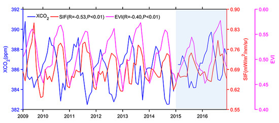
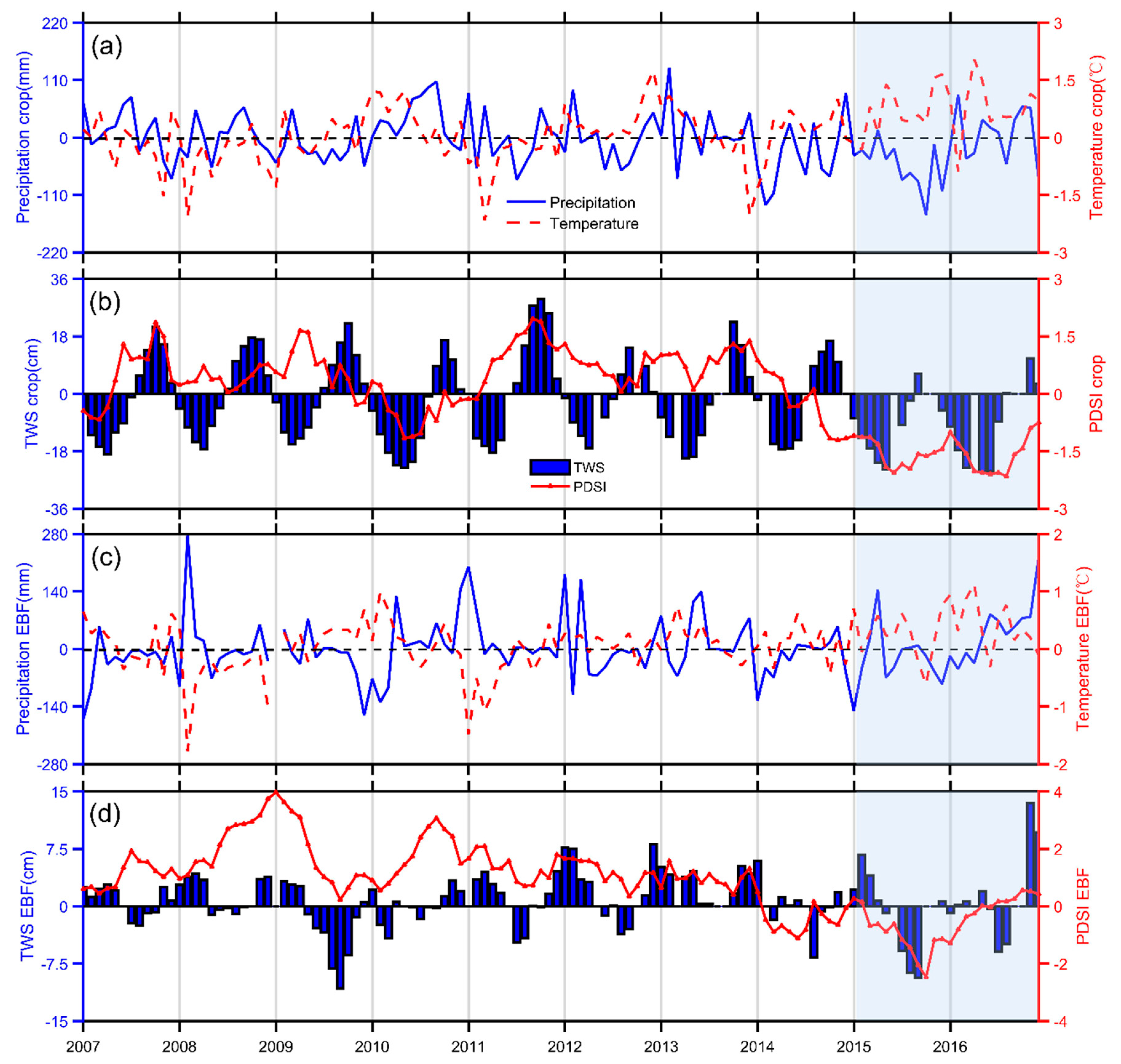
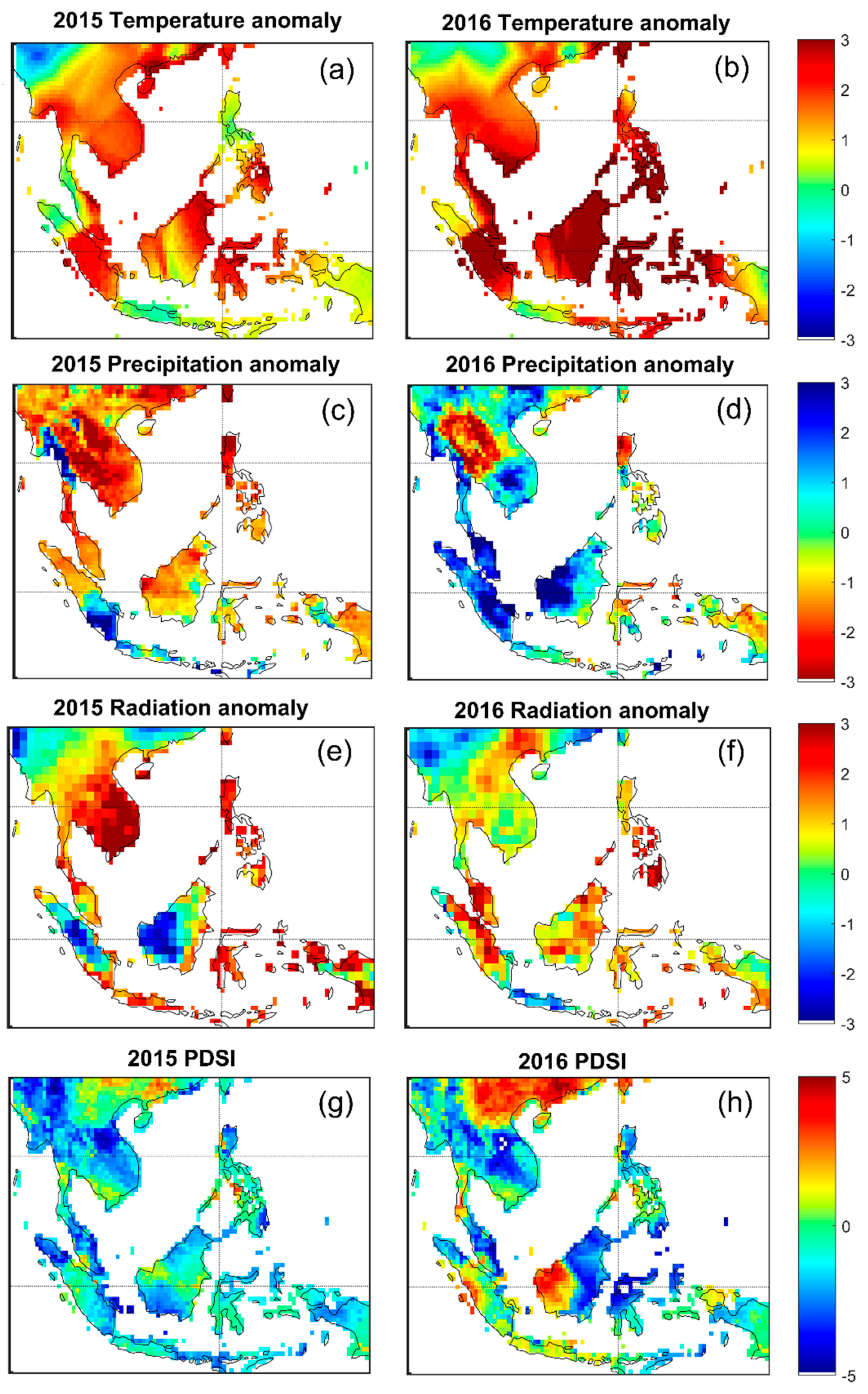
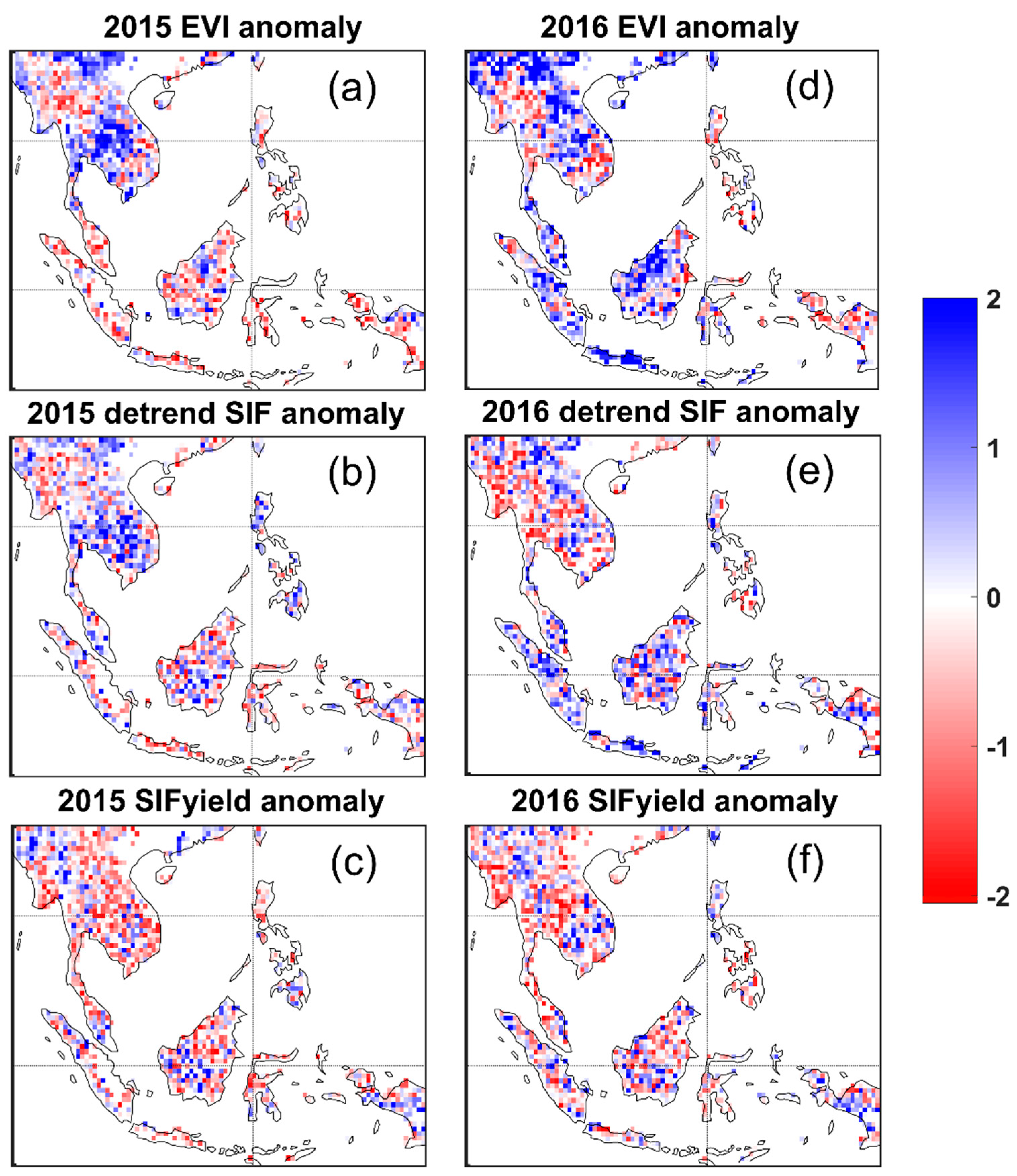
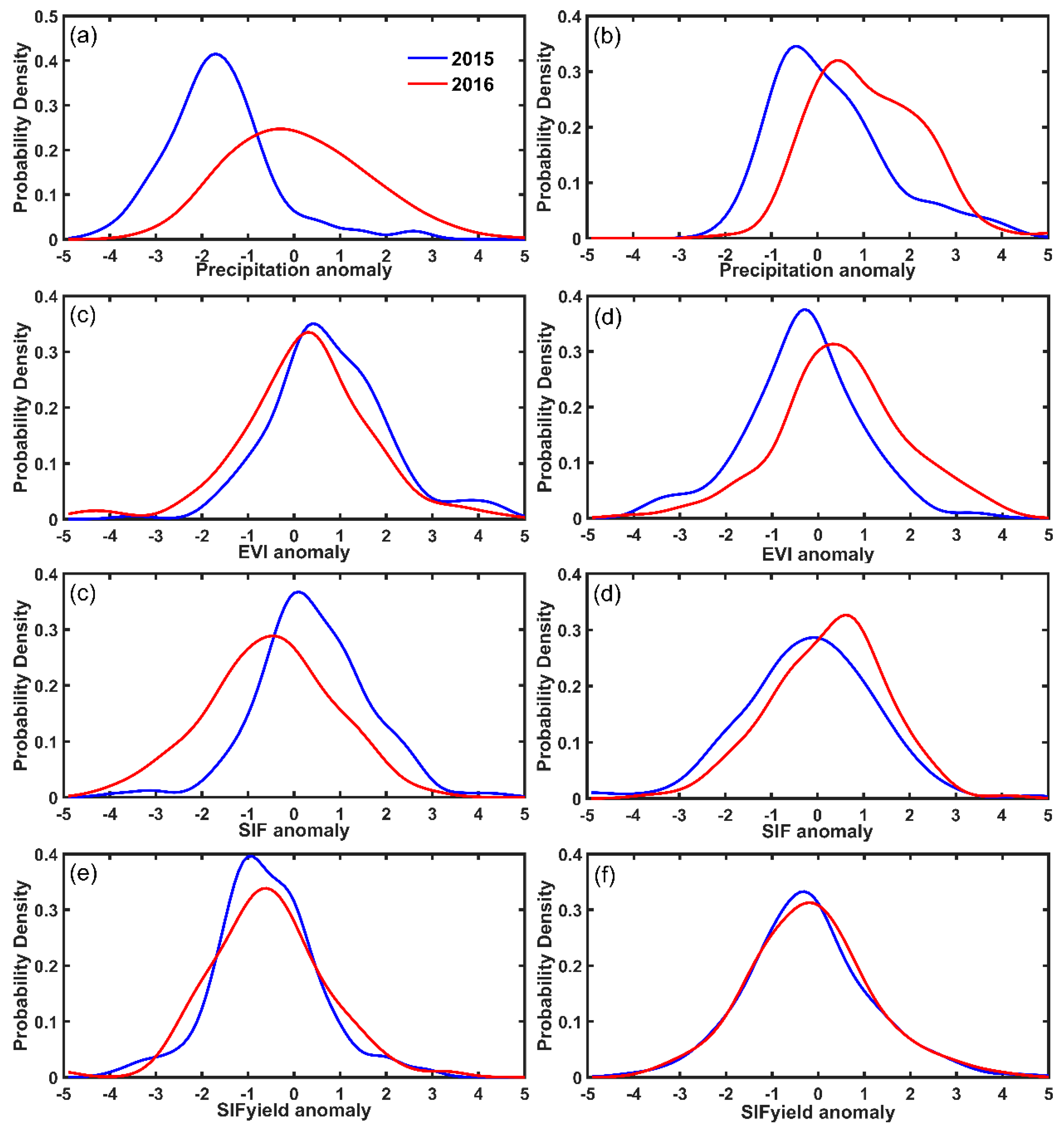
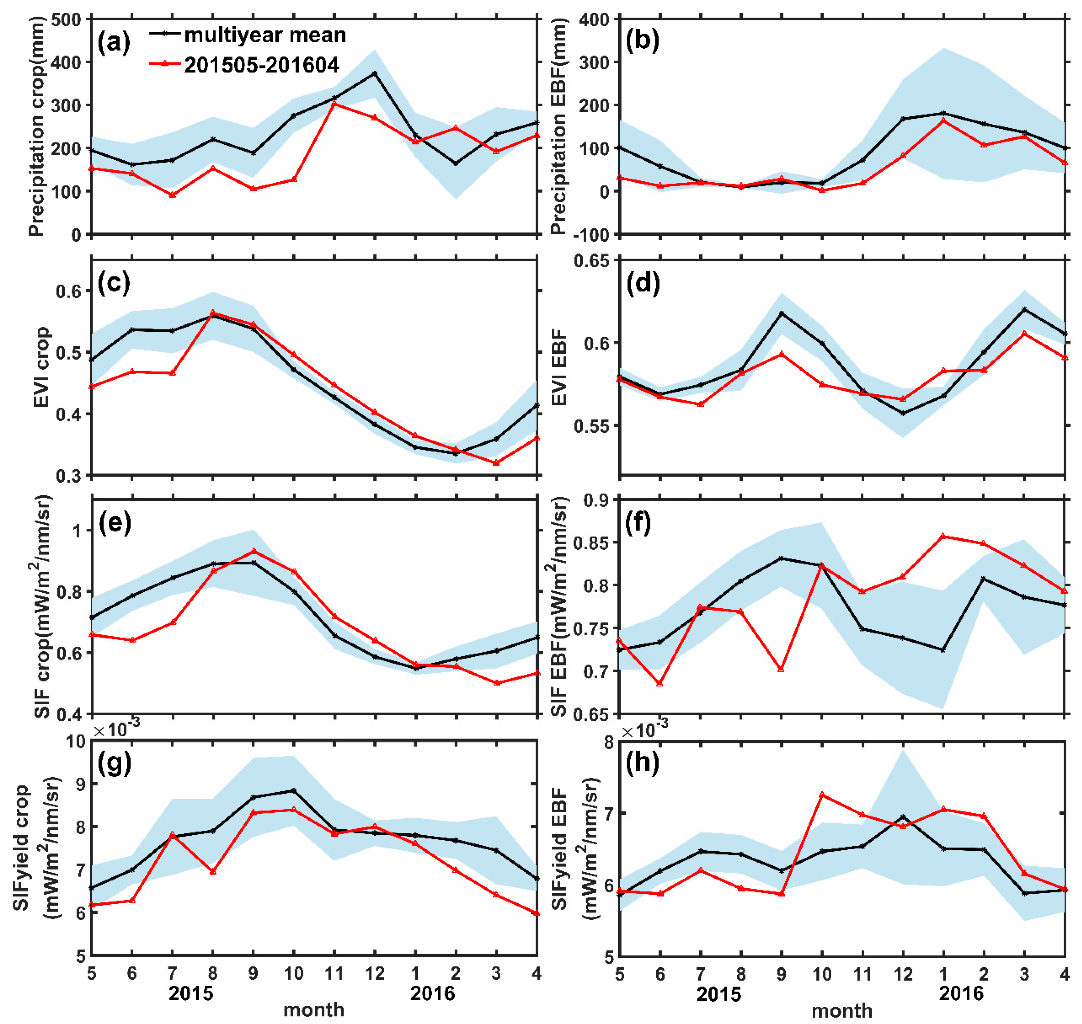
3. Results
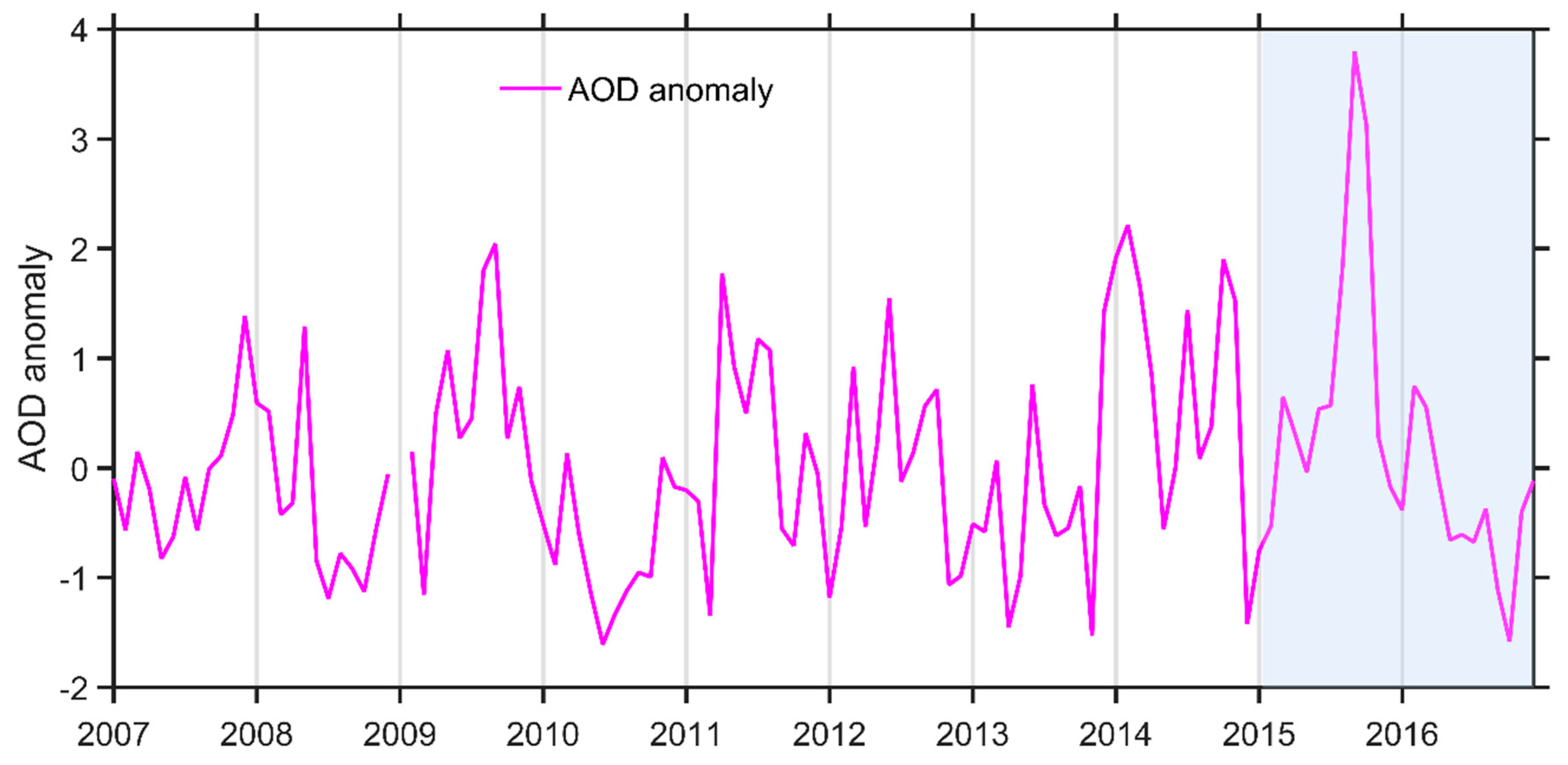
3.1. The 2015/16 Drought
3.2. Response of Vegetation to Drought
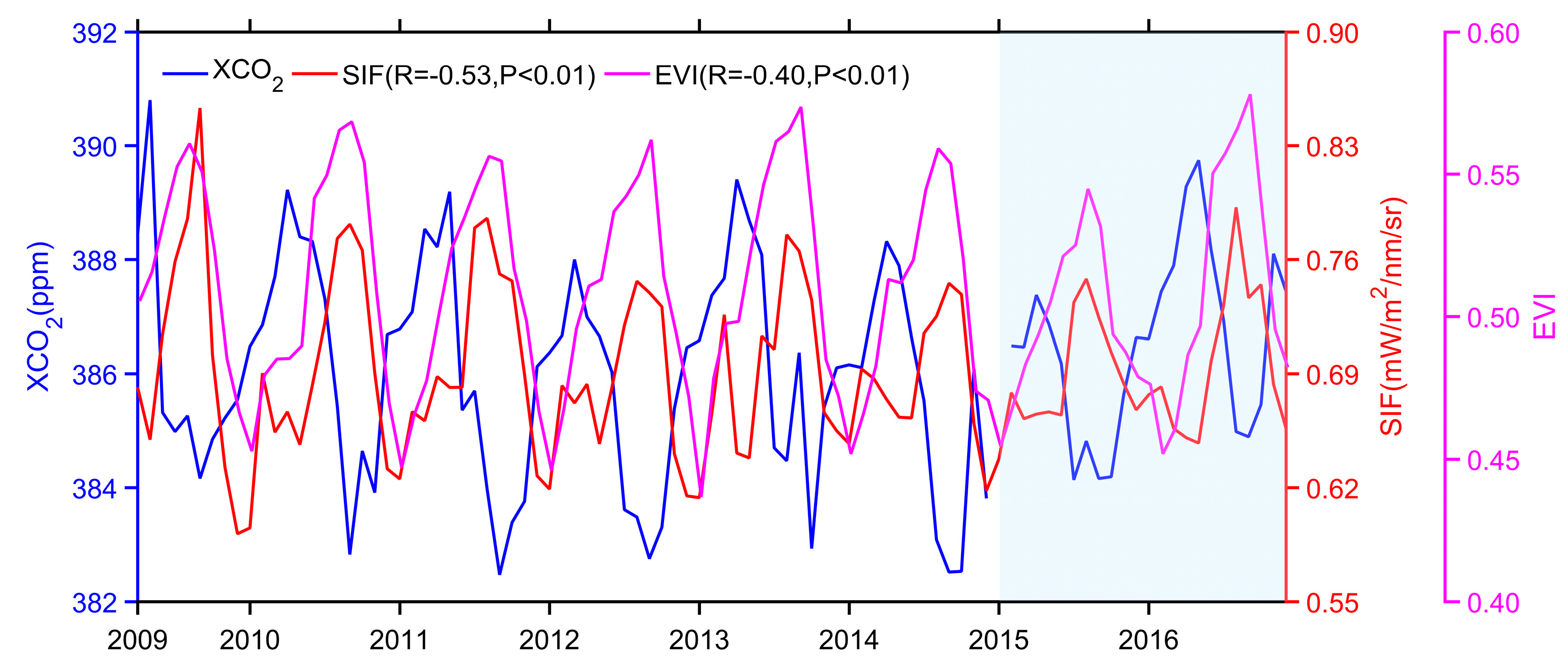
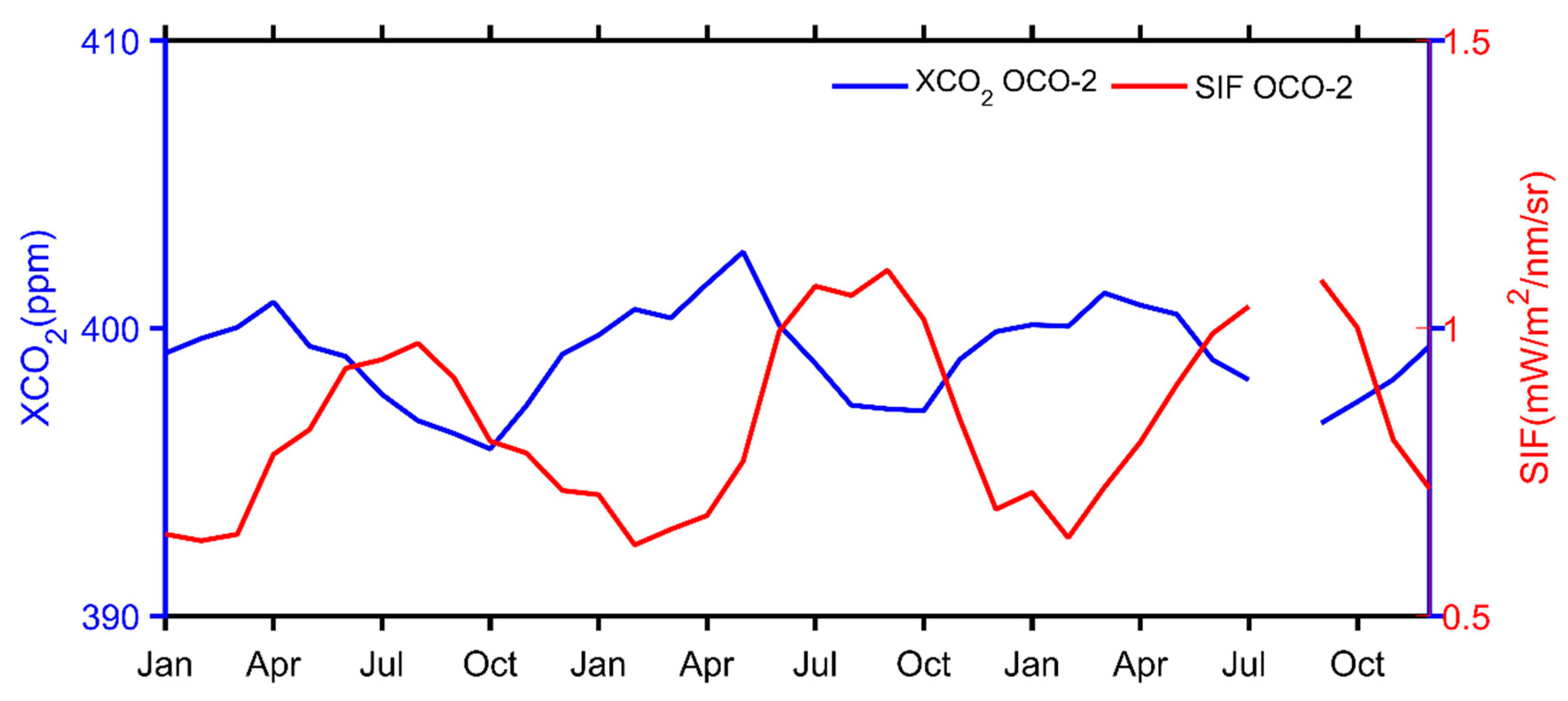
3.3. Implications on the Regional Carbon Cycle
4. Conclusions and Discussion
Author Contributions
Funding
Acknowledgments
Conflicts of Interest
References
- Detmers, R.; Hasekamp, O.; Aben, I.; Houweling, S.; Van Leeuwen, T.; Butz, A.; Landgraf, J.; Köhler, P.; Guanter, L.; Poulter, B. Anomalous carbon uptake in Australia as seen by GOSAT. Geophys. Res. Lett. 2015, 42, 8177–8184. [Google Scholar] [CrossRef]
- Page, S.E.; Siegert, F.; Rieley, J.O.; Boehm, H.-D.V.; Jaya, A.; Limin, S. The amount of carbon released from peat and forest fires in Indonesia during 1997. Nature 2002, 420, 61. [Google Scholar] [CrossRef]
- Reichstein, M.; Bahn, M.; Ciais, P.; Frank, D.; Mahecha, M.D.; Seneviratne, S.I.; Zscheischler, J.; Beer, C.; Buchmann, N.; Frank, D.C. Climate extremes and the carbon cycle. Nature 2013, 500, 287. [Google Scholar] [CrossRef] [PubMed]
- Glikson, A. Cenozoic mean greenhouse gases and temperature changes with reference to the Anthropocene. Glob. Chang. Biol. 2016, 22, 3843–3858. [Google Scholar] [CrossRef]
- Blunden, J.; Arndt, D.S. State of the climate in 2015. Bull. Am. Meteorol. Soc. 2016, 97, S275. [Google Scholar] [CrossRef]
- Huijnen, V.; Wooster, M.J.; Kaiser, J.W.; Gaveau, D.L.; Flemming, J.; Parrington, M.; Inness, A.; Murdiyarso, D.; Main, B.; van Weele, M. Fire carbon emissions over maritime southeast Asia in 2015 largest since 1997. Sci. Rep. 2016, 6, 26886. [Google Scholar] [CrossRef]
- Jiménez-Muñoz, J.C.; Mattar, C.; Barichivich, J.; Santamaría-Artigas, A.; Takahashi, K.; Malhi, Y.; Sobrino, J.A.; Van Der Schrier, G. Record-breaking warming and extreme drought in the Amazon rainforest during the course of El Niño 2015–2016. Sci. Rep. 2016, 6, 33130. [Google Scholar] [CrossRef] [PubMed]
- Wang, Y.; Xie, Y.; Dong, W.; Ming, Y.; Wang, J.; Shen, L. Adverse effects of increasing drought on air quality via natural processes. Atmos. Chem. Phys. 2017, 17, 12827–12843. [Google Scholar] [CrossRef]
- Van Der Schrier, G.; Klein Tank, A.M.; Van Den Besselaar, E.J.; Swarinoto, Y. Observed trends and variability in climate indices relevant for crop yields in Southeast Asia. J. Clim. 2016, 29, 2651–2669. [Google Scholar]
- Peng, J.; Dadson, S.; Leng, G.; Duan, Z.; Jagdhuber, T.; Guo, W.; Ludwig, R. The impact of the Madden-Julian Oscillation on hydrological extremes. J. Hydrol. 2019, 571, 142–149. [Google Scholar] [CrossRef]
- Mu, Q.; Zhao, M.; Kimball, J.S.; McDowell, N.G.; Running, S.W. A remotely sensed global terrestrial drought severity index. Bull. Am. Meteorol. Soc. 2013, 94, 83–98. [Google Scholar] [CrossRef]
- Tucker, C.J.; Choudhury, B.J. Satellite remote sensing of drought conditions. Remote Sens. Environ. 1987, 23, 243–251. [Google Scholar] [CrossRef]
- Gu, Y.; Brown, J.F.; Verdin, J.P.; Wardlow, B. A five-year analysis of MODIS NDVI and NDWI for grassland drought assessment over the central Great Plains of the United States. Geophys. Res. Lett. 2007, 34, L06407. [Google Scholar] [CrossRef]
- Huete, A.; Didan, K.; Miura, T.; Rodriguez, E.P.; Gao, X.; Ferreira, L.G. Overview of the radiometric and biophysical performance of the MODIS vegetation indices. Remote Sens. Environ. 2002, 83, 195–213. [Google Scholar] [CrossRef]
- Lee, J.-E.; Frankenberg, C.; van der Tol, C.; Berry, J.A.; Guanter, L.; Boyce, C.K.; Fisher, J.B.; Morrow, E.; Worden, J.R.; Asefi, S. Forest productivity and water stress in Amazonia: Observations from GOSAT chlorophyll fluorescence. Proc. R. Soc. Biol. Sci. 2013, 280, 20130171. [Google Scholar] [CrossRef] [PubMed]
- Zhou, L.; Tian, Y.; Myneni, R.B.; Ciais, P.; Saatchi, S.; Liu, Y.Y.; Piao, S.; Chen, H.; Vermote, E.F.; Song, C. Widespread decline of Congo rainforest greenness in the past decade. Nature 2014, 509, 86. [Google Scholar] [CrossRef]
- Asner, G.P.; Alencar, A. Drought impacts on the Amazon forest: The remote sensing perspective. New Phytol. 2010, 187, 569–578. [Google Scholar] [CrossRef]
- Daumard, F.; Champagne, S.; Fournier, A.; Goulas, Y.; Ounis, A.; Hanocq, J.-F.; Moya, I. A field platform for continuous measurement of canopy fluorescence. IEEE Trans. Geosci. Remote Sens. 2010, 48, 3358–3368. [Google Scholar] [CrossRef]
- Zarco-Tejada, P.J.; Miller, J.R.; Mohammed, G.H.; Noland, T.L.; Sampson, P.H. Chlorophyll fluorescence effects on vegetation apparent reflectance: II. Laboratory and airborne canopy-level measurements with hyperspectral data. Remote Sens. Environ. 2000, 74, 596–608. [Google Scholar] [CrossRef]
- Frankenberg, C.; Fisher, J.B.; Worden, J.; Badgley, G.; Saatchi, S.S.; Lee, J.E.; Toon, G.C.; Butz, A.; Jung, M.; Kuze, A. New global observations of the terrestrial carbon cycle from GOSAT: Patterns of plant fluorescence with gross primary productivity. Geophys. Res. Lett. 2011, 38, L17706. [Google Scholar] [CrossRef]
- Guanter, L.; Rossini, M.; Colombo, R.; Meroni, M.; Frankenberg, C.; Lee, J.-E.; Joiner, J. Using field spectroscopy to assess the potential of statistical approaches for the retrieval of sun-induced chlorophyll fluorescence from ground and space. Remote Sens. Environ. 2013, 133, 52–61. [Google Scholar] [CrossRef]
- Joiner, J.; Guanter, L.; Lindstrot, R.; Voigt, M.; Vasilkov, A.; Middleton, E.; Huemmrich, K.; Yoshida, Y.; Frankenberg, C. Global monitoring of terrestrial chlorophyll fluorescence from moderate-spectral-resolution near-infrared satellite measurements: Methodology, simulations, and application to GOME-2. Atmos. Meas. Tech. 2013, 6, 2803–2823. [Google Scholar] [CrossRef]
- Joiner, J.; Yoshida, Y.; Vasilkov, A.; Middleton, E. First observations of global and seasonal terrestrial chlorophyll fluorescence from space. Biogeosciences 2011, 8, 637–651. [Google Scholar] [CrossRef]
- Guanter, L.; Zhang, Y.; Jung, M.; Joiner, J.; Voigt, M.; Berry, J.A.; Frankenberg, C.; Huete, A.R.; Zarco-Tejada, P.; Lee, J.-E. Global and time-resolved monitoring of crop photosynthesis with chlorophyll fluorescence. Proc. Natl. Acad. Sci. USA 2014, 111, E1327–E1333. [Google Scholar] [CrossRef]
- Zhang, Y.; Guanter, L.; Berry, J.A.; van der Tol, C.; Yang, X.; Tang, J.; Zhang, F. Model-based analysis of the relationship between sun-induced chlorophyll fluorescence and gross primary production for remote sensing applications. Remote Sens. Environ. 2016, 187, 145–155. [Google Scholar] [CrossRef]
- Song, L.; Guanter, L.; Guan, K.; You, L.; Huete, A.; Ju, W.; Zhang, Y. Satellite sun-induced chlorophyll fluorescence detects early response of winter wheat to heat stress in the Indian Indo-Gangetic Plains. Glob. Chang. Biol. 2018, 24, 4023–4037. [Google Scholar] [CrossRef]
- Shan, N.; Ju, W.; Migliavacca, M.; Martini, D.; Guanter, L.; Chen, J.; Goulas, Y.; Zhang, Y. Modeling canopy conductance and transpiration from solar-induced chlorophyll fluorescence. Agric. For. Meteorol. 2019, 268, 189–201. [Google Scholar] [CrossRef]
- Qiu, B.; Li, W.; Wang, X.; Shang, L.; Song, C.; Guo, W.; Zhang, Y. Satellite-observed solar-induced chlorophyll fluorescence reveals higher sensitivity of alpine ecosystems to snow cover on the Tibetan Plateau. Agric. For. Meteorol. 2019, 271, 126–134. [Google Scholar] [CrossRef]
- Sun, Y.; Fu, R.; Dickinson, R.; Joiner, J.; Frankenberg, C.; Gu, L.; Xia, Y.; Fernando, N. Drought onset mechanisms revealed by satellite solar-induced chlorophyll fluorescence: Insights from two contrasting extreme events. J. Geophys. Res. Biogeosci. 2015, 120, 2427–2440. [Google Scholar] [CrossRef]
- Yoshida, Y.; Joiner, J.; Tucker, C.; Berry, J.; Lee, J.-E.; Walker, G.; Reichle, R.; Koster, R.; Lyapustin, A.; Wang, Y. The 2010 Russian drought impact on satellite measurements of solar-induced chlorophyll fluorescence: Insights from modeling and comparisons with parameters derived from satellite reflectances. Remote Sens. Environ. 2015, 166, 163–177. [Google Scholar] [CrossRef]
- Zhang, L.; Qiao, N.; Huang, C.; Wang, S. Monitoring Drought Effects on Vegetation Productivity Using Satellite Solar-Induced Chlorophyll Fluorescence. Remote Sens. 2019, 11, 378. [Google Scholar] [CrossRef]
- Grainger, A. Difficulties in tracking the long-term global trend in tropical forest area. Proce. Natl. Acad. Sci. USA 2008, 105, 818–823. [Google Scholar] [CrossRef] [PubMed]
- Saatchi, S.S.; Harris, N.L.; Brown, S.; Lefsky, M.; Mitchard, E.T.; Salas, W.; Zutta, B.R.; Buermann, W.; Lewis, S.L.; Hagen, S. Benchmark map of forest carbon stocks in tropical regions across three continents. Proc. Natl. Acad. Sci. USA 2011, 108, 9899–9904. [Google Scholar] [CrossRef] [PubMed]
- Huete, A.R.; Didan, K.; Shimabukuro, Y.E.; Ratana, P.; Saleska, S.R.; Hutyra, L.R.; Yang, W.; Nemani, R.R.; Myneni, R. Amazon rainforests green-up with sunlight in dry season. Geophys. Res. Lett. 2006, 33, L06405. [Google Scholar] [CrossRef]
- Guan, K.; Pan, M.; Li, H.; Wolf, A.; Wu, J.; Medvigy, D.; Caylor, K.K.; Sheffield, J.; Wood, E.F.; Malhi, Y. Photosynthetic seasonality of global tropical forests constrained by hydroclimate. Nat. Geosci. 2015, 8, 284. [Google Scholar] [CrossRef]
- Liu, J.; Bowman, K.W.; Schimel, D.S.; Parazoo, N.C.; Jiang, Z.; Lee, M.; Bloom, A.A.; Wunch, D.; Frankenberg, C.; Sun, Y. Contrasting carbon cycle responses of the tropical continents to the 2015–2016 El Niño. Science 2017, 358, eaam5690. [Google Scholar] [CrossRef] [PubMed]
- Harris, I.; Jones, P.D.; Osborn, T.J.; Lister, D.H. Updated high-resolution grids of monthly climatic observations-the CRU TS3.10 Dataset. Int. J. Climatol. 2014, 34, 623–642. [Google Scholar] [CrossRef]
- Duncan, B.N.; Prados, A.I.; Lamsal, L.N.; Liu, Y.; Streets, D.G.; Gupta, P.; Hilsenrath, E.; Kahn, R.A.; Nielsen, J.E.; Beyersdorf, A.J. Satellite data of atmospheric pollution for US air quality applications: Examples of applications, summary of data end-user resources, answers to FAQs, and common mistakes to avoid. Atmos. Environ. 2014, 94, 647–662. [Google Scholar] [CrossRef]
- Wahr, J.; Swenson, S.; Zlotnicki, V.; Velicogna, I. Time-variable gravity from GRACE: First results. Geophys. Res. Lett. 2004, 31, L11501. [Google Scholar] [CrossRef]
- Save, H.; Bettadpur, S.; Tapley, B.D. High-resolution CSR GRACE RL05 mascons. J. Geophys. Res. Solid Earth 2016, 121, 7547–7569. [Google Scholar] [CrossRef]
- Wayne, C.P. Meteorological drought. Res. Pap. 1965, 45, 58. [Google Scholar]
- Karl, T.R.; Quayle, R.G. The 1980 summer heat wave and drought in historical perspective. Mon. Wea. Rev. 1981, 109, 2055–2073. [Google Scholar] [CrossRef]
- Wells, N.; Goddard, S.; Hayes, M.J. A self-calibrating Palmer drought severity index. J. Clim. 2004, 17, 2335–2351. [Google Scholar] [CrossRef]
- Van der Schrier, G.; Barichivich, J.; Briffa, K.; Jones, P. A scPDSI-based global data set of dry and wet spells for 1901–2009. J. Geophys. Res. Atmos. 2013, 118, 4025–4048. [Google Scholar] [CrossRef]
- Crisp, D.; Pollock, H.R.; Rosenberg, R.; Chapsky, L.; Lee, R.A.; Oyafuso, F.A.; Frankenberg, C.; O‘Dell, C.W.; Bruegge, C.J.; Doran, G.B. The on-orbit performance of the Orbiting Carbon Observatory-2 (OCO-2) instrument and its radiometrically calibrated products. Atmos. Meas. Tech. 2017, 10, 59–81. [Google Scholar] [CrossRef]
- O’Dell, C.; Connor, B.; Bösch, H.; O’Brien, D.; Frankenberg, C.; Castano, R.; Christi, M.; Eldering, A.; Fisher, B.; Gunson, M. The ACOS CO2 Retrieval Algorithm—Part 1: Description and Validation Against Synthetic Observations. Atmos. Meas. Tech. 2012, 5, 99–121. [Google Scholar]
- Köhler, P.; Guanter, L.; Joiner, J. A Linear Method for the Retrieval of Sun-Induced Chlorophyll Fluorescence from GOME-2 and SCIAMACHY Data. Atmos. Meas. Tech. 2015, 8, 2589–2608. [Google Scholar] [CrossRef]
- Joiner, J.; Yoshida, Y.; Guanter, L.; Middleton, E.M. New methods for the retrieval of chlorophyll red fluorescence from hyperspectral satellite instruments: Simulations and application to GOME-2 and SCIAMACHY. Atmos. Meas. Tech. 2016, 9, 3939–3967. [Google Scholar] [CrossRef]
- Duysens, L.; Sweers, H. Mechanism of the Two Photochemical Reactions in Algae as Studied by Means of Fluorescence; Miyachi, S.: Tokyo, Japan, 1963; pp. 353–372. [Google Scholar]
- Walther, S.; Guanter, L.; Heim, B.; Jung, M.; Duveiller, G.; Wolanin, A.; Sachs, T. Assessing the dynamics of vegetation productivity in circumpolar regions with different satellite indicators of greenness and photosynthesis. Biogeosciences 2018, 15, 6221–6256. [Google Scholar] [CrossRef]
- Cox, P.M.; Pearson, D.; Booth, B.B.; Friedlingstein, P.; Huntingford, C.; Jones, C.D.; Luke, C.M. Sensitivity of tropical carbon to climate change constrained by carbon dioxide variability. Nature 2013, 494, 341. [Google Scholar] [CrossRef]
- Qiu, B.; Xue, Y.; Fisher, J.B.; Guo, W.; Berry, J.A.; Zhang, Y. Satellite Chlorophyll Fluorescence and Soil Moisture Observations Lead to Advances in the Predictive Understanding of Global Terrestrial Coupled Carbon-Water Cycles. Glob. Biogeochem. Cycles 2018, 32, 360–375. [Google Scholar] [CrossRef]
- Keppel-Aleks, G.; Wolf, A.S.; Mu, M.; Doney, S.C.; Morton, D.C.; Kasibhatla, P.S.; Miller, J.B.; Dlugokencky, E.J.; Randerson, J.T. Separating the influence of temperature, drought, and fire on interannual variability in atmospheric CO2. Glob. Biogeochem. Cycles 2014, 28, 1295–1310. [Google Scholar] [CrossRef] [PubMed]
- Keenan, T.; Baker, I.; Barr, A.; Ciais, P.; Davis, K.; Dietze, M.; Dragoni, D.; Gough, C.M.; Grant, R.; Hollinger, D. Terrestrial biosphere model performance for inter-annual variability of land-atmosphere CO2 exchange. Glob. Chang. Biol. 2012, 18, 1971–1987. [Google Scholar] [CrossRef]
- Lopes, A.P.; Nelson, B.W.; Wu, J.; de Alencastro Graça, P.M.L.; Tavares, J.V.; Prohaska, N.; Martins, G.A.; Saleska, S.R. Leaf flush drives dry season green-up of the Central Amazon. Remote Sens. Environ. 2016, 182, 90–98. [Google Scholar] [CrossRef]
- Wu, J.; Albert, L.P.; Lopes, A.P.; Restrepo-Coupe, N.; Hayek, M.; Wiedemann, K.T.; Guan, K.; Stark, S.C.; Christoffersen, B.; Prohaska, N. Leaf development and demography explain photosynthetic seasonality in Amazon evergreen forests. Science 2016, 351, 972–976. [Google Scholar] [CrossRef]
- Qiu, B.; Guo, W.; Xue, Y.; Dai, Q. Implementation and evaluation of a generalized radiative transfer scheme within canopy in the soil-vegetation-atmosphere transfer (SVAT) model. J. Geophys. Res. Atmos. 2016, 121, 12145–12163. [Google Scholar] [CrossRef]
- Betts, R.A.; Jones, C.D.; Knight, J.R.; Keeling, R.F.; Kennedy, J.J.; Wiltshire, A.J.; Andrew, R.M.; Aragão, L.E. A successful prediction of the record CO2 rise associated with the 2015/2016 El Nino. Philos. Trans. R. Soc. Biol. Sci. 2018, 373, 20170301. [Google Scholar] [CrossRef]
- Laan-Luijkx, I.; Velde, I.; Krol, M.; Gatti, L.; Domingues, L.; Correia, C.; Miller, J.; Gloor, M.; Leeuwen, T.; Kaiser, J. Response of the Amazon carbon balance to the 2010 drought derived with CarbonTracker South America. Glob. Biogeochem. Cycles 2015, 29, 1092–1108. [Google Scholar] [CrossRef]
- Doughty, C.E.; Goulden, M.L. Are tropical forests near a high temperature threshold? J. Geophys. Res. Biogeosci. 2008, 113, G00B07. [Google Scholar] [CrossRef]
- Yang, J.; Tian, H.; Pan, S.; Chen, G.; Zhang, B.; Dangal, S. Amazon drought and forest response: Largely reduced forest photosynthesis but slightly increased canopy greenness during the extreme drought of 2015/2016. Glob. Chang. Biol. 2018, 24, 1919–1934. [Google Scholar] [CrossRef]
- Koren, G.; van Schaik, E.; Araújo, A.C.; Boersma, K.F.; Gärtner, A.; Killaars, L.; Kooreman, M.L.; Kruijt, B.; van der Laan-Luijkx, I.T.; von Randow, C. Widespread reduction in sun-induced fluorescence from the Amazon during the 2015/2016 El Niño. Philos. Trans. R. Soc. Biol. Sci. 2018, 373, 20170408. [Google Scholar] [CrossRef] [PubMed]
- Wang, X.; Piao, S.; Ciais, P.; Friedlingstein, P.; Myneni, R.B.; Cox, P.; Heimann, M.; Miller, J.; Peng, S.; Wang, T. A two-fold increase of carbon cycle sensitivity to tropical temperature variations. Nature 2014, 506, 212. [Google Scholar] [CrossRef] [PubMed]
- Luo, X.; Keenan, T.F.; Fisher, J.B.; Jiménez-Muñoz, J.-C.; Chen, J.M.; Jiang, C.; Ju, W.; Perakalapudi, N.-V.; Ryu, Y.; Tadić, J.M. The impact of the 2015/2016 El Niño on global photosynthesis using satellite remote sensing. Philos. Trans. R. Soc. Biol. Sci. 2018, 373, 20170409. [Google Scholar] [CrossRef] [PubMed]


© 2019 by the authors. Licensee MDPI, Basel, Switzerland. This article is an open access article distributed under the terms and conditions of the Creative Commons Attribution (CC BY) license (http://creativecommons.org/licenses/by/4.0/).
Share and Cite
Qian, X.; Qiu, B.; Zhang, Y. Widespread Decline in Vegetation Photosynthesis in Southeast Asia Due to the Prolonged Drought During the 2015/2016 El Niño. Remote Sens. 2019, 11, 910. https://doi.org/10.3390/rs11080910
Qian X, Qiu B, Zhang Y. Widespread Decline in Vegetation Photosynthesis in Southeast Asia Due to the Prolonged Drought During the 2015/2016 El Niño. Remote Sensing. 2019; 11(8):910. https://doi.org/10.3390/rs11080910
Chicago/Turabian StyleQian, Xin, Bo Qiu, and Yongguang Zhang. 2019. "Widespread Decline in Vegetation Photosynthesis in Southeast Asia Due to the Prolonged Drought During the 2015/2016 El Niño" Remote Sensing 11, no. 8: 910. https://doi.org/10.3390/rs11080910
APA StyleQian, X., Qiu, B., & Zhang, Y. (2019). Widespread Decline in Vegetation Photosynthesis in Southeast Asia Due to the Prolonged Drought During the 2015/2016 El Niño. Remote Sensing, 11(8), 910. https://doi.org/10.3390/rs11080910