Theoretical Evaluation of Water Cloud Model Vegetation Parameters

Abstract

The advantage of implementing the Water Cloud Model (WCM) is in being able to express complex scattering characteristics in a vegetated area with simple bulk vegetation descriptors. However, there has been a lack of understanding or consensus about the optimal set of vegetation descriptors. In this paper, the original and improved expressions of WCM are evaluated and the optimal vegetation descriptors are presented by examining the relationship between WCM vegetation parameters and the theoretical scattering model predictions. In addition, the condition-specific regression relationship between bulk vegetation descriptors and theoretical scattering and attenuation coefficients, expressed by the $A$ and $B$ parameters in the WCM, is analyzed in relation to the shape, size, and orientation distribution of the scatterer. Furthermore, the influence of radar observation conditions on the parameterization of the WCM is presented. The results show that the particle moisture content and the vegetation water content can be the optimal vegetation descriptors, denoted by the $V_1$ and $V_2$ variables in the WCM, respectively.

1. Introduction

Due to its all-weather imaging and vegetation penetration capabilities, remote sensing of vegetated areas with Synthetic Aperture Radar (SAR) has a great potential for retrieving bio- and geo-physical parameters related to vegetation and the underlying soil surface. The measured SAR signal backscattered from natural targets is given by the superposition of many elementary scatterers. Consequently, in order to estimate physical properties of scatterers from SAR data, it is necessary to investigate different scattering contributions among total backscattered signals by modeling the interactions of microwaves in the vegetated areas.

Theoretical scattering models, such as the discrete scattering model [1,2] and the radiative transfer model [3,4,5], have been used to assess the relative importance of microwave scattering mechanisms. In the theoretical models, the vegetation canopy is, in general, represented as an ensemble of randomly distributed dielectric particles, in a layer of specific height, overlying a dielectric ground layer. The total backscatter can be obtained by an incoherent sum of several scattering contributions, including direct backscattering from the vegetation layer, direct backscattering from the underlying rough surface, scattering interaction between the vegetation and the ground surface, and ground–vegetation–ground multiple bounce. The theoretical scattering models have been used successfully to interpret scattering characteristics of vegetated areas and to predict radar signals in relation to the biophysical properties of plants. However, they are usually complex and inconvenient because of a large number of input parameters which lead to complexity in resolving the inverse problem.

To ascertain physical properties of vegetation and soil, a semi-empirical model named the Water Cloud Model (WCM), was proposed [6]. In the WCM, the canopy is assumed to be a uniform cloud of water like particles. Then, the total backscattered signal is expressed in simplified form, such as an incoherent sum of the backscattering contributions of the uniform canopy layer and the underlying rough surface. Since the canopy in the WCM can be represented by one or two bulk vegetation parameters, it can be practically used for retrieving physical properties. Several studies have used the WCM for soil moisture estimation over vegetated areas [7,8,9,10,11] and for biophysical parameter estimation [12].

In the practical application of WCM, however, parameterization of the simplified model has been the main problem due to the heterogeneity of actual land surface. The WCM tries to express the canopy scattering and attenuation terms in the model by simple vegetation parameters. Several bulk parameters, including Vegetation Water Content (VWC) [8,9,10,11,12,13], Leaf Area Index (LAI) [7,9,11], biomass [12], and plant water content [12], have been used as the vegetation descriptors in the literature. Nonetheless, there have been few studies on the selection of the optimal vegetation descriptors in the WCM. Another problem in the parameterization of the WCM is that two unknown model parameters, which relate vegetation descriptors to microwave scattering and attenuation in the canopy layer, have to be determined prior to performing inversion. Studies on retrieving land surface parameters provided site-specific model parameters by regression analysis using field experimental data [7,8,9,10,11,12]. Recently, there were some studies particularly interested in determining model parameters in the WCM, the named calibration of the WCM, for L-band [13] and C-band [14,15,16,17] space-borne SAR systems by using in-situ and optical remote sensing data.

This study is dedicated to discussing the aforementioned problems in the parameterization of the WCM. In this paper, the original and improved expressions of WCM are examined and the optimal set of bulk vegetation descriptors is evaluated by using the theoretical model. In addition, the condition-specific regression relationship between bulk vegetation descriptors and theoretical scattering and attenuation coefficients will be analyzed in relation to the vegetation structure. Furthermore, the influence of radar observation conditions on the parameterization of the WCM is investigated. In Section 2, we review the WCM and discuss how the bulk vegetation descriptors are related to the WCM parameters. Section 3 presents the effects of shape, size, and orientation of vegetation elements on the parameterization of the WCM. The sensitivity of WCM parameters to observation conditions is discussed concludes this paper in Section 4 and Section 5.

2. Water Cloud Model

The Water Cloud Model represents a vegetation layer as a collection of identical spherical particles, uniformly distributed throughout the volume layer. The total backscattering coefficient, ${\sigma }^0$, can be expressed by the incoherent sum of the scattering contribution of the vegetation layer, ${\mathsf{\sigma }}_v^0$, and the scattering contribution of the soil layer, ${\mathsf{\sigma }}_s^0$, attenuated by the attenuation coefficient $T^2$, given as follows:

$${\sigma }^0={\mathsf{\sigma }}_v^0+{\mathsf{\sigma }}_s^0{T}^2,$$

(1)

$${\mathsf{\sigma }}_v^0=\frac{{\sigma }_v\cos \theta }{2{\kappa }_e}\left[1-T^2\right],$$

(2)

$$T^2=\exp (-2{\kappa }_{e}h/\cos \theta ),$$

(3)

where ${\sigma }_v$ and ${\kappa }_e$ are the volume backscattering and extinction coefficients of the vegetation layer, $h$ is the vegetation height, $\theta$ is the incidence angle, and ${\mathsf{\sigma }}_s^0$ is the soil backscattering coefficient. Neglecting multiple scattering effects, ${\sigma }_v$ and ${\kappa }_e$, can be given by the sum of the backscattering cross section, $S$, and the extinction cross section, $k$, of a single particle, such as

$${\sigma }_v=NS \mathrm{and} {\kappa }_e=Nk,$$

(4)

where $N$ is the number of particles per unit volume (m⁻³). The simplification of the vegetation layer permits the relation of the scattering characteristics to bulk vegetation parameters. In the case of uniformly distributed water particles, the extinction coefficient can be assumed to be proportional to the total water content in the unit volume $W$ (kg/m³), such as [6]

$${\kappa }_e=B_{1}W.$$

(5)

In a similar way, the ratio ${\sigma }_v/2{\kappa }_e$, which determines the vegetation backscattering coefficient, can be assumed to be independent of water content, such as

$$\frac{{\sigma }_v}{2{\kappa }_e}=A_1.$$

(6)

However, the simple expressions for the scattering and extinction coefficients in Equations (5) and (6) are only valid for the cloud of water particles. In order to apply the simple vegetation model to practical SAR observations, many researches have used more general expression [7,8,9,10,11,12,13,14,15,16], such as

$${\sigma }^0=A_2{V}_1\cos \theta \left[1-\exp (-2B_2{V}_2/\cos \theta )\right]+{\mathsf{\sigma }}_s^0\exp (-2B_2{V}_2/\cos \theta ).$$

(7)

The unknown coefficients $A_2$ and $B_2$ in the general WCM can be dependent on the canopy type. Since there have been no theoretical basis to determine $A_2$ and $B_2$, they need to be empirically determined. The scattering and extinction coefficients are represented by bulk vegetation parameters $V_1$ and $V_2$. Due to the heterogeneity of vegetation structure, several different sets of vegetation parameters have been proposed in the literature, e.g., VWC, LAI, canopy height ($h$), and particle moisture content ($m_g$).

In order to examine the best set of vegetation parameters and the corresponding $A_2$ and $B_2$, let us firstly assume a vegetation layer consisting of cloud of spherical dielectric particles. The backscattering and extinction cross sections for a spherical Rayleigh scatterer of radius, $r$, and dielectric constant, ${\epsilon }_v$, are [18]

$$S=\frac{128{\pi }^5{r}^6}{3{\lambda }^4}{|\frac{1-{\epsilon }_v}{{\epsilon }_v+2}|}^2, \mathrm{and}$$

(8)

$$k=\frac{8{\pi }^2{r}^3}{\lambda }\mathrm{Im}(\frac{1-{\epsilon }_v}{{\epsilon }_v+2}).$$

(9)

Here, the dielectric constant of a particle, ${\epsilon }_v$, can be related to the gravimetric moisture content, $m_g$, through the Ulaby and El-Rayes model [19], where

$$m_g=\frac{W_w-W_d}{W_w}.$$

(10)

$W_w$ and $W_d$ are the wet and dry mass of a particle. By comparing Equations (1)–(3) and (7), the $A_2{V}_1$ and the $B_2{V}_2$ terms can be expressed as follows:

$$A_2{V}_1=\frac{S}{2k}=\frac{8{\pi }^3{r}^3}{3{\lambda }^3}{|\frac{{\epsilon }_v-1}{{\epsilon }_v+2}|}^2/\mathrm{Im}(\frac{{\epsilon }_v-1}{{\epsilon }_v+2}), \mathrm{and}$$

(11)

$$B_2{V}_2=kNh=\frac{8{\pi }^2{r}^3}{\lambda }\mathrm{Im}(\frac{{\epsilon }_v-1}{{\epsilon }_v+2})Nh.$$

(12)

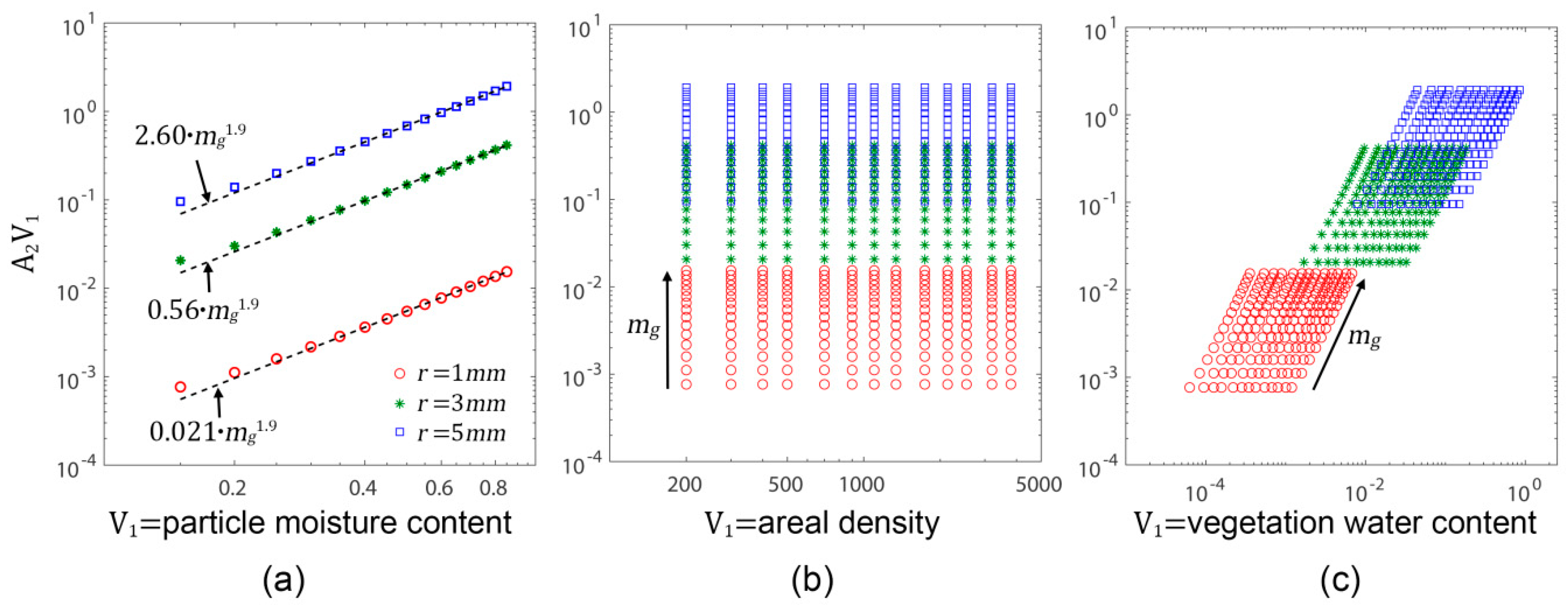
To understand the coefficients $A_2$ and $B_2$ and the vegetation parameters $V_1$ and $V_2$, variations of $A_2{V}_1$ and $B_2{V}_2$ terms are examined in relation to several vegetation descriptors, such as the particle moisture content, $m_g$, the areal density, $N_a$ (m⁻²), and the VWC (kg/m²), as shown in Figure 1 and Figure 2. The areal density and VWC are defined as

$$N_a=Nh,$$

(13)

$$\mathrm{VWC}=(W_w-W_d)Nh=m_g{\rho }_w{v}_p{N}_a,$$

(14)

where ${\rho }_w$ is the particle wet density ($~500$ kg/m³, [20]) and particle volume $v_p=(4\pi /3)r^3$.

Figure 1 and Figure 2 show calculated $A_2{V}_1$ and $B_2{V}_2$ parameters plotted against different vegetation descriptors. The dielectric constant, ${\epsilon }_v$, for calculating WCM parameters is derived from the Ulaby and EL-Rayes model at 5 GHz. It is shown that the $A_2{V}_1$ term is highly related to $m_g$, while it is independent of particle density. Since it exhibits a quadratic-like dependence on $m_g$, the $A_2{V}_1$ term can be rewritten in relation to $m_g$, such as

$$A_2{V}_1\approx A_2{m}_g^E.$$

(15)

Here, the coefficient $A_2$ varies with the particle size. According to the least square method, $A_2$ varies from 0.021 for $r=\lambda /50$ to 2.6 for $r=\lambda /10$, while $E=1.9$ independently with the particle size. On the contrary, the $B_2{V}_2$ term exhibits a linear relationship with VWC, as shown in Figure 2. In this case, we can rewrite the $B_2{V}_2$ term as

$$B_2{V}_2=B_2\mathrm{VWC}=\frac{6\pi {10}^{-3}}{\lambda }\mathrm{Im}(\frac{{\epsilon }_v-1}{{\epsilon }_v+2})\frac{1}{m_g} \mathrm{VWC}.$$

(16)

The coefficient $B_2$ is not a constant but determined by the moisture content of particles. It varies from 0.27 for dry particles ($m_g= 0.1$) to 0.014 for wet particles ($m_g= 0.9$).

3. WCM Parameters for Non-Spherical Particles

The WCM tries to express complicated canopy backscatters in terms of a small number of vegetation parameters. However, the WCM with identical spherical particles predicts identical co-polarization and no cross-polarization backscatters, which are far from the real SAR observables. In order to figure out more realistic WCM model parameters, backscatter simulations with physical models considering non-spherical particles are presented in this section.

Based on the solution of the radiative transfer equation [3,4,5], the pq-polarization backscattering contribution of the vegetation layer can be written as

$${\mathsf{\sigma }}_{v,pq}^0=\frac{{\sigma }_{v,pq}\cos \theta }{2{\kappa }_{e,pq}}\left[1-\exp (-2{\kappa }_{e,pq}h/\cos \theta )\right].$$

(17)

In the case of a canopy layer consisting of randomly oriented dielectric non-spherical particles assuming identical size and shape, the volume scattering coefficient, ${\sigma }_{v,pq}$, and the extinction coefficient, ${\kappa }_{e,pq}$, can be obtained by statistical averaging over the scatterer’s orientation distribution $p(\alpha ,\beta )$, such as

$${\sigma }_{v,pp}=N\langle {|S_{pq}(\widehat{s},\widehat{i})|}^2\rangle =N{{\displaystyle \int }}^{}{{\displaystyle \int }}^{}P(\alpha ,\beta ){|S_{pq}(\widehat{s},\widehat{i})|}^{2}d\alpha d\beta ,$$

(18)

$${\kappa }_{e,pq}=0.5N\{\langle k_q(-\widehat{i})\rangle +N\langle k_p(\widehat{i})\rangle \}.$$

(19)

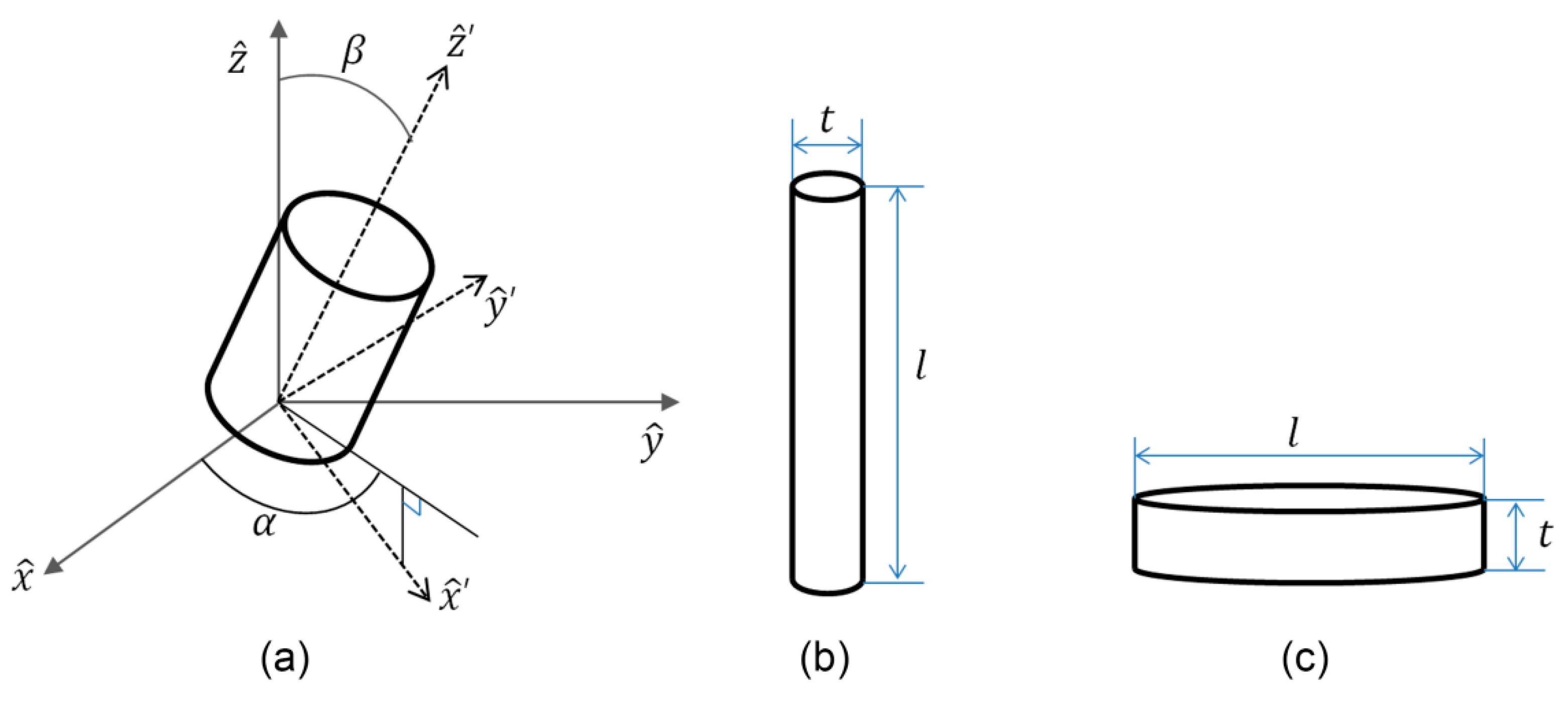
The orientation distribution of the azimuthal angle, $\alpha$, and the inclination angle, $\beta$, are shown in Figure 3a. All scatterers are assumed to be distributed uniformly in the azimuth, such as $p(\alpha )=1/2\pi$. For a small non-spherical particle, the scattering amplitude, $S_{pq}(\widehat{s},\widehat{i})$, on the incident, $\widehat{i}$, and scattered, $\widehat{s}$, directions and the extinction cross section, $k_p(\widehat{i})$, can be calculated by using the Generalized Rayleigh-Gans (GRG) approximation [21]. It has been widely used (e.g., [22,23,24,25]) for modeling radar scattering properties from leaves. To evaluate the effects of particle shape, size, and orientation on the parameterization of WCM, two types of vegetation, composed of needle shaped (Figure 3b) and circular disk shaped (Figure 3c) particles, are considered in this study.

3.1. Effect of Particle Shape

For non-spherical particles, the constants $A_2$ and $B_2$ will vary with polarization. In this study, polarization dependent model parameters will be examined for co-polarization cases, since the cross-polarization signal generally contains no scattering contribution from the soil surface, which has been of great interest in WCM applications. The polarization dependent model constants $A_{2,pq}$ and $B_{2,pq}$ can be estimated by fitting WCM parameters to the simulation results of the GRG-based physical model. The WCM components are related to the vegetation attenuation and scattering terms of the physical model as

$${\kappa }_{e,pq}h\approx B_{2,pq}{V}_2,$$

(20)

$$\frac{{\sigma }_{v,pq}}{2{\kappa }_{e,pq}}\approx A_{2,pq}{V}_1.$$

(21)

The volume scattering and the extinction coefficients in the left-hand side of the equation are calculated by the GRG approximation. A number of scattering and extinction coefficients of different vegetation, composed of either needles or disks, are simulated using the parameters given in

Table 1. Vegetation parameters used in the GRG-based model simulation.

Vegetation Parameter	Minimum	Maximum	Interval	Unit
Particle length ($l$)	3	24	3	cm
Number density ($N$)	200	4200	400	m−3
Height ($h$)	1	5	1	m
Particle moisture content ($m_g$)	0.1	0.9	0.1	g/g

. In the simulation, the thickness ($t$) of needles and disks are set to be 0.1 cm and 0.01 cm, respectively. In addition to the uniform azimuth angle distribution, all scatterers are assumed to be distributed uniformly in the inclination angles, in the calculation of the GRG-based model.

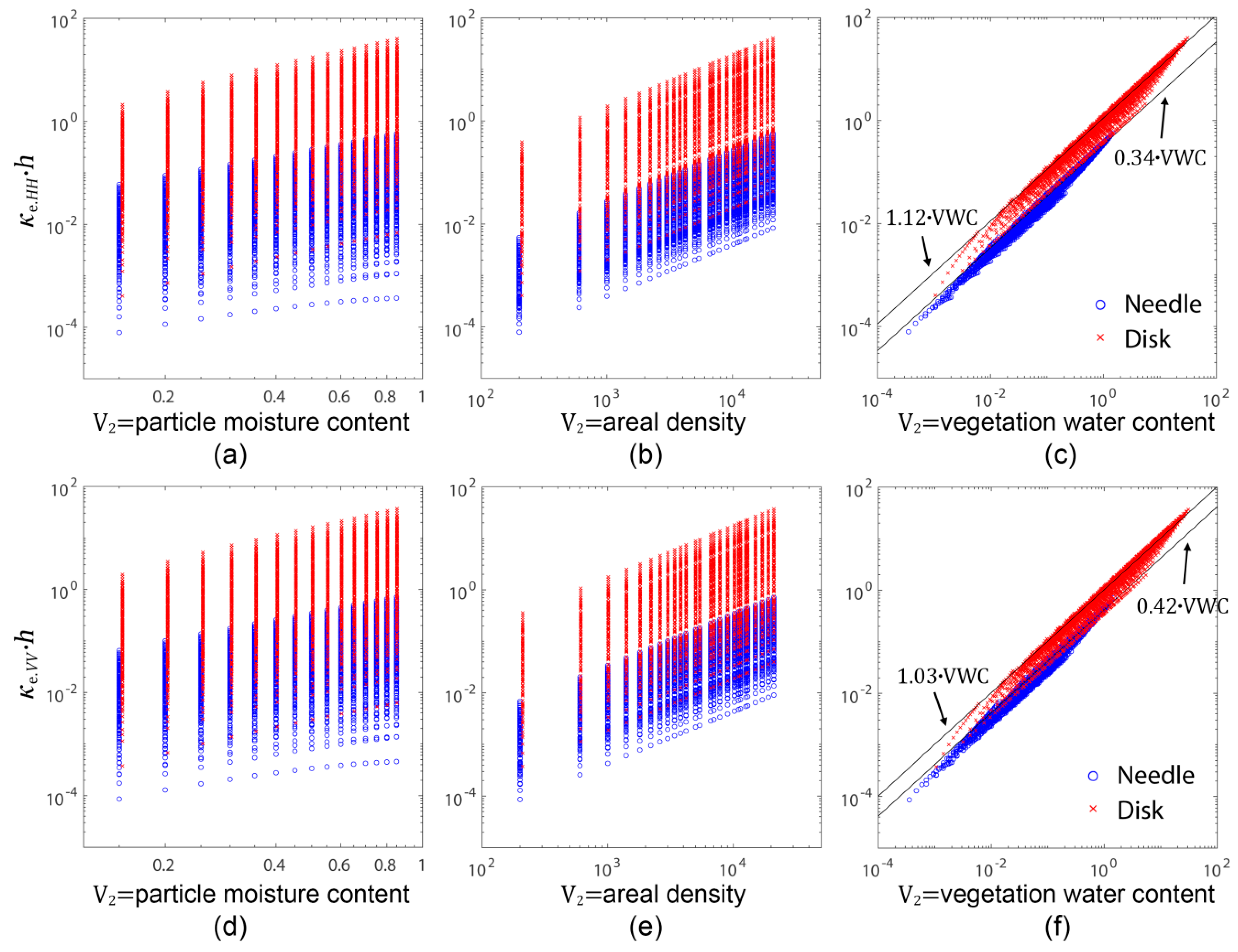
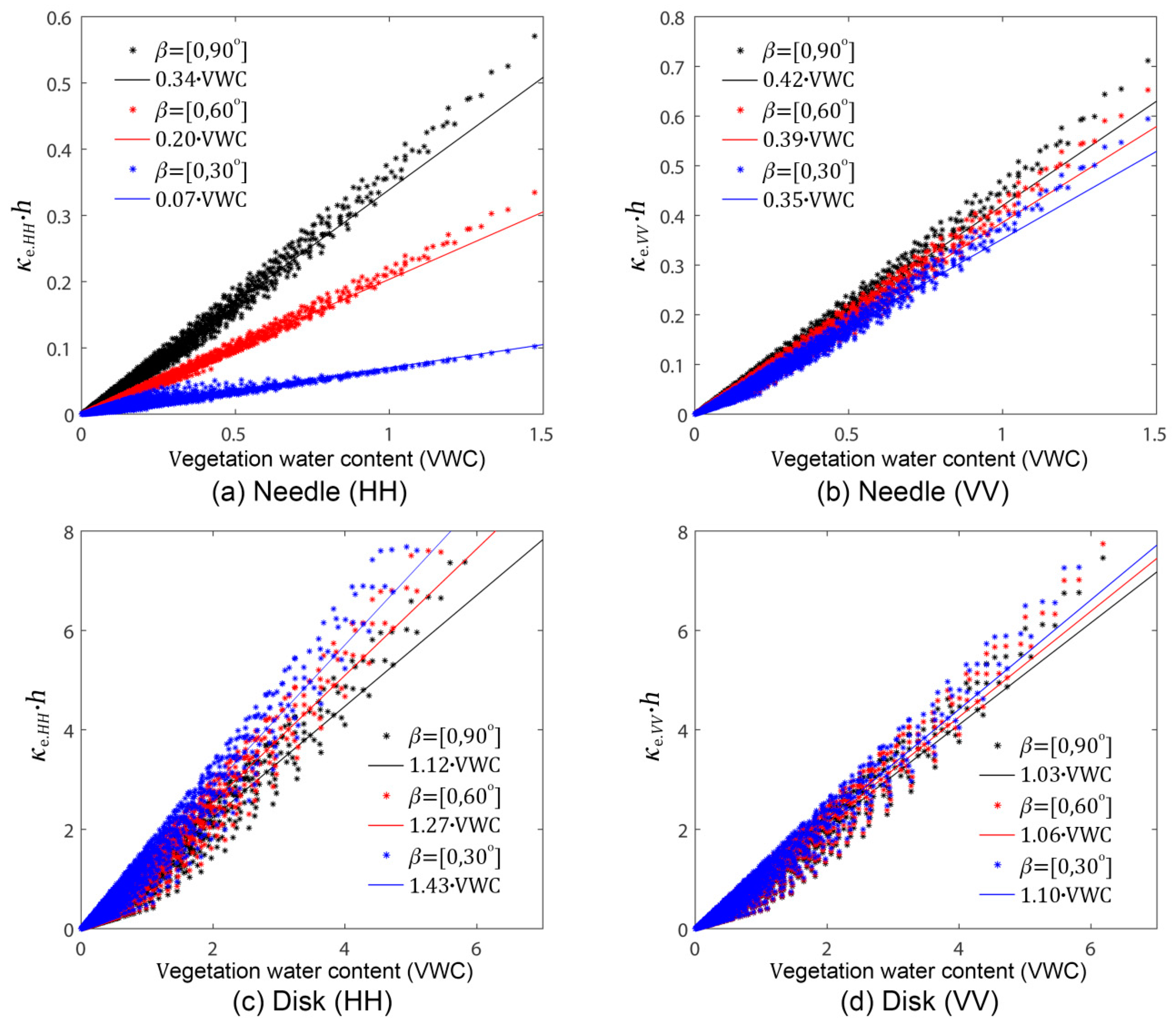
Figure 4 illustrates variations of ${\kappa }_{e,HH}h$ and ${\kappa }_{e,VV}h$ terms by the GRG-based model with respect to different vegetation descriptors, such as $m_g$, $N_a$, and VWC. The simulation is performed at 5 GHz frequency. It shows a strong linear relationship between ${\kappa }_{e,pq}h$ terms and VWC in both HH- and VV-polarizations, regardless of the particle shape. Consequently, the VWC is selected as the optimal $V_2$ parameter and the corresponding $B_{2,pq}$ coefficient can be determined by the slope of the least square line. Results show that the particle shape affects significantly on the $B_{2,pq}$ coefficients of the WCM. A vegetation canopy composed of disk-shaped particles is described by a higher $B_{2,pq}$ coefficient than if it is composed of needle shaped particles. In addition, despite the uniform distribution assumption, the estimated $B_{2,HH}$ is slightly higher than $B_{2,VV}$ in the case of disk-shaped particles. On the other hand, in the case of needle shaped particles, the estimated $B_{2,VV}$ is slightly higher than $B_{2,HH}$.

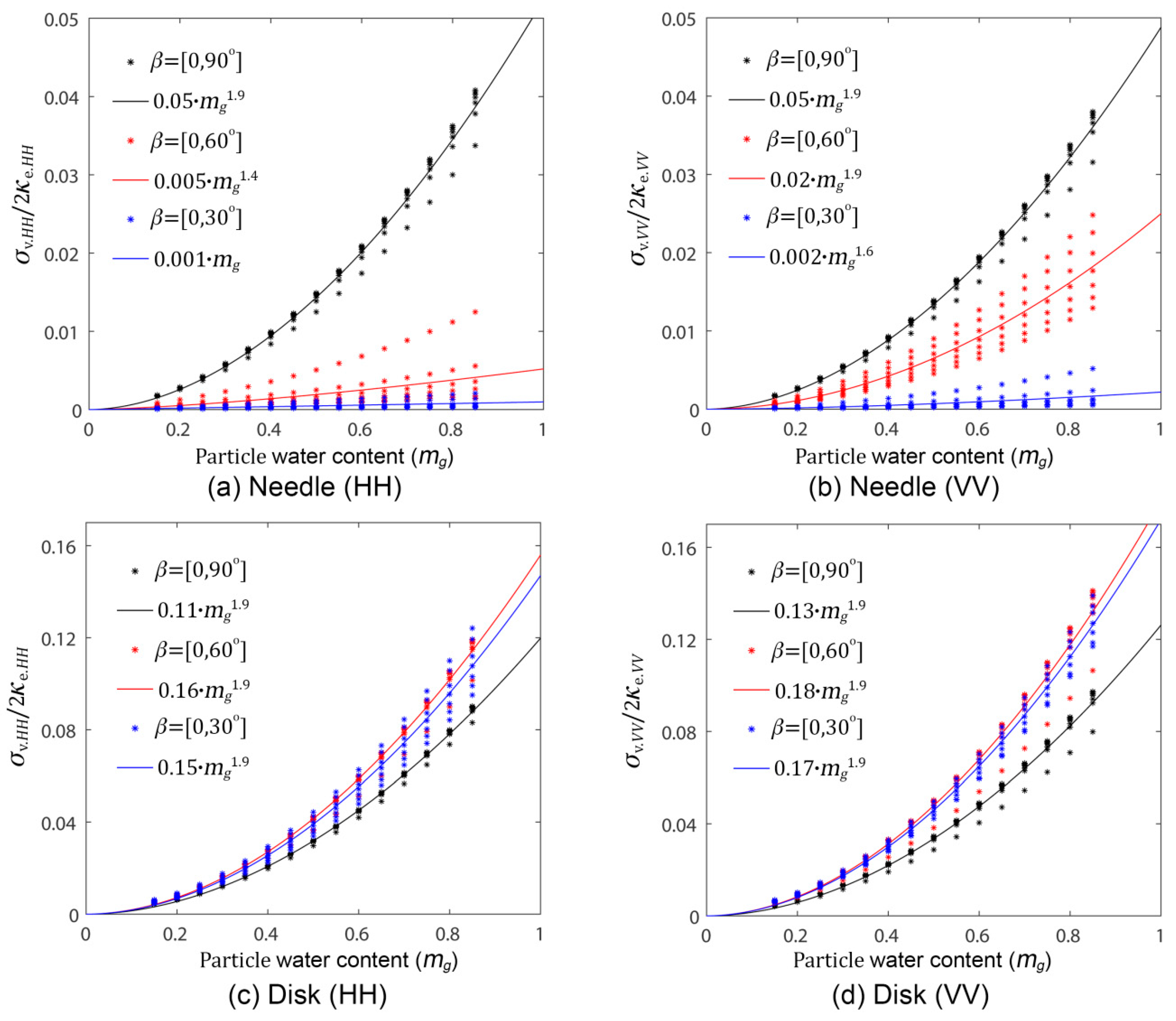
To determine the $V_1$ parameter and to estimate corresponding $A_{2,pq}$ coefficients, variations of the ${\sigma }_{v,pq}/2{\kappa }_{e,pq}$ terms are examined against different vegetation descriptors, as shown in Figure 5. As with the spherical particle, the ${\sigma }_{v,pq}/2{\kappa }_{e,pq}$ is strongly correlated with the $m_g$ and exhibits a quadratic-like relationship. Based on a non-linear expression, such as

$$\frac{{\sigma }_{v,pq}}{2{\kappa }_{e,pq}}\approx A_{2,pq}{m}_g^E,$$

(22)

the $A_{2,pq}$ and $E$ parameters can be estimated by least square fit. The estimated $E$ is about 1.9 independently with the particle shape, size, and density. The estimated model coefficient $A_{2,pq}$ is affected by particle shape. The disk shaped particle exhibits higher $A_{2,pq}$ than the needle shaped scatter. The model coefficients at HH- and VV-polarizations, $A_{2,HH}$ and $A_{2,VV}$, are not significantly different in both the disk and needle shaped particles.

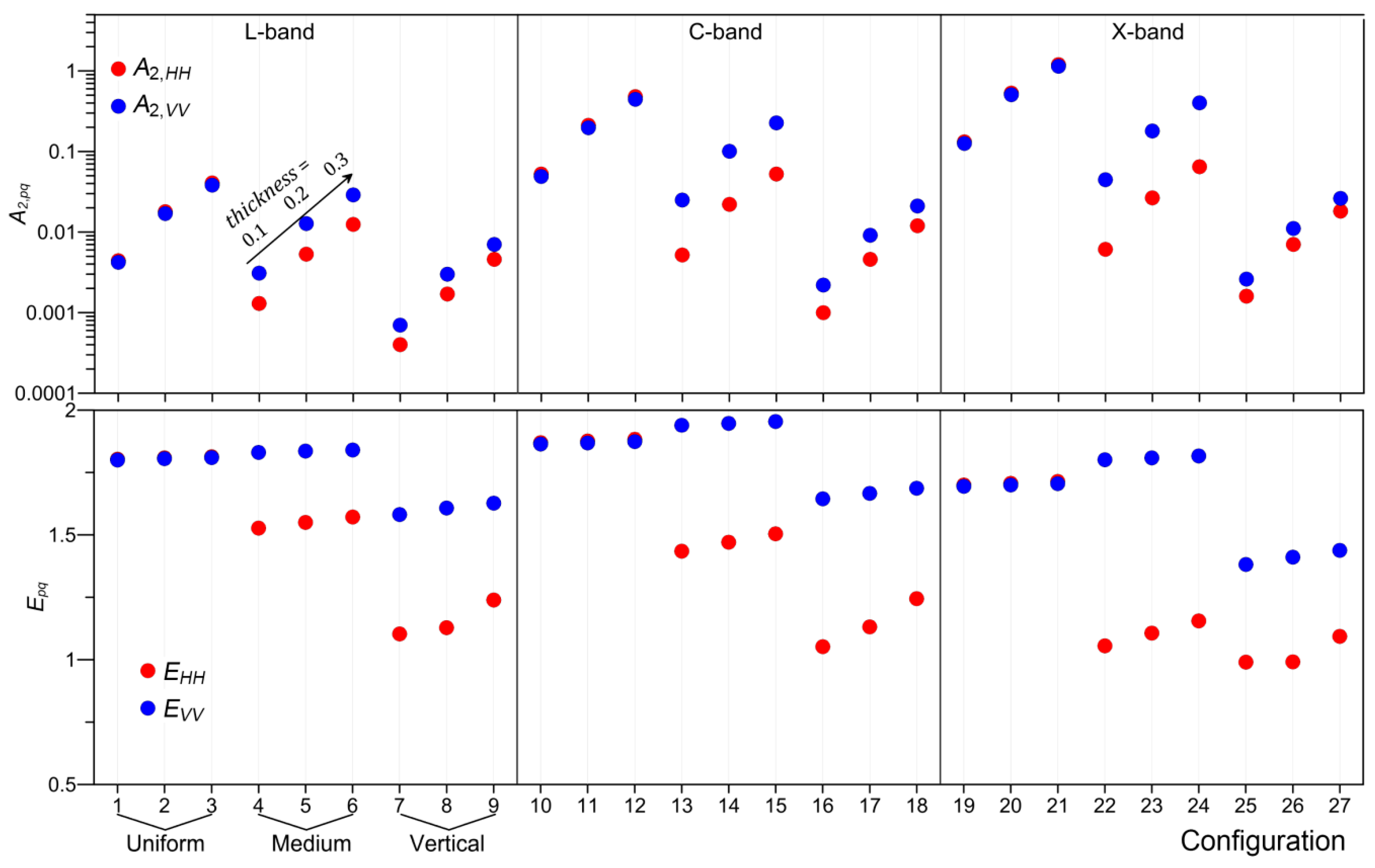
3.2. Effect of Particle Orientation

In the previous experiment, non-spherical particles are assumed to be uniformly distributed throughout vegetation layer. However, in many agricultural crops and forests, the scatterers in a volume layer may have a preferred orientation distribution. In order to consider more realistic vegetation structure in the parameterization of WCM, scattering and attenuation coefficients from particles with preferred orientation distribution are considered in this part. The distribution of the inclination angle $p(\beta$) is used to denote the orientation of particles. For simplicity, it is assumed to be a uniform distribution over the interval ${\beta }_1\le \beta \le {\beta }_2$, such as $P(\beta )=1/({\beta }_2-{\beta }_1)$. When $\beta$ varies in a range around 0°, the needle shaped particles are vertically oriented, while the disk-shaped particles are nearly horizontal.

Figure 6 shows variations of the $B_{2,pq}$ coefficients in the oriented volume. Based on previous analysis, VWC is selected for the vegetation descriptor $V_2$ and $B_{2,pq}$ is obtained by fitting the linear function. For the inclination distribution, we consider the three following special cases: $0{}^{{}^{°}}\le \beta \le 90{}^{°}$, $0{}^{°}\le \beta \le 60{}^{°}$, and $0{}^{°}\le \beta \le 30{}^{°}$. The first case corresponds to the uniform inclination angle distribution, as with the previous experiment. The third case corresponds to either nearly vertically oriented needle or nearly horizontally oriented disk particles.

It is seen from Figure 6 that the linear relationship between ${\kappa }_{e,pq}h$ terms and VWC is maintained throughout different orientation distributions. However, for horizontal disks and vertical needles, oriented volume effects in wave propagation through vegetation layer lead to the differences of the $B_{2,pq}$ coefficients between HH- and VV-polarizations. Particularly, the $B_{2,HH}$ coefficient, which is associated to the attenuation of HH-polarized signal, is more affected by the orientation of the scatterer than the $B_{2,VV}$ coefficient. In comparing needle and disk-shaped particles, the orientation angle effect is more significant in the needle shaped particle. The $B_{2,HH}$ coefficient decreases significantly as the needle shaped particle is oriented vertically.

Next, the effect of particle orientation on the $A_{2,pq}$ coefficients is evaluated in Figure 7. As in the previous analysis, $m_g^E$ is used for the vegetation descriptor. As with the $B_{2,pq}$ coefficients, orientation distribution affects the $A_{2,pq}$ coefficients of the needle shaped particle more, especially at HH-polarization. The estimated $A_{2,pq}$ coefficients decrease significantly as the needle shaped particles are oriented vertically. In addition, it is seen that the estimated $E$ parameter is influenced by the particle orientation distribution and becomes dependent on the radar polarization. It decreases from 1.9 for uniform distribution to 1.0 in HH-polarization and 1.6 in VV-polarization for the vertically oriented needle. On the other hand, the orientation distribution hardly affects the $E$ parameter in the case of disk shaped particles. The estimated $A_{2,pq}$ coefficients slightly decrease as the disk is oriented horizontally.

4. Discussion

4.1. Effect of Radar Observation Condition

Two experiments in the previous section discussed parameterization of the WCM in relation to the shape and orientation of scatterers. In addition to the environmental condition of the scatterer, however, radar observation parameters affect the unknown model constants in the WCM. In particular, radar scattering mechanisms in vegetated areas can be sensitive to the incidence angle and the frequency of the transmitted signal. In order to further evaluate the effect of observation conditions, we analyzed the model parameters of WCM that were estimated under different incidence angles and frequencies of the radar signal.

Figure 8 shows dependence of the estimated model parameters on the incidence angle and frequency. As with the estimation procedure discussed in the previous section, the model parameters were determined by fitting $B_{2,pq}\mathrm{VWC}$ and $A_{2,pq}{m}_g^E$ terms in the WCM to the simulation results of the GRG-based physical model. In this figure, the shape and orientation distribution of scatterers were kept constant, such as the moderately vertical ($0{}^{°}\le \beta \le 60{}^{°}$) needle shaped scatterers. In addition, according to the previous analysis, the E parameter in the WCM may also depend on the radar polarization. Therefore, the $E$ parameter for the non-linear fitting was replaced by the polarization dependent parameter $E_{pq}$.

Figure 8a–c illustrates the variations of model parameters as a function of the incidence angle. It is seen that the $B_{2,VV}$ parameter increases as an increase of the incidence angle, while the $B_{2,HH}$ parameter is not affected by the incidence angle variation. The $A_{2,pq}$ parameters increase as an increase of the incidence angle. The estimated $A_{2,pq}$ is consistently higher for the HH-polarization case than the VV-polarization case. In addition, the difference between $A_{2,HH}$ and $A_{2,VV}$ is larger at a high incidence angle region. The estimated $E_{pq}$ parameters are not very sensitive to the incidence angle as compared to other WCM parameters. The $E_{HH}$ parameter is consistently higher than the $E_{VV}$ parameters.

On the other hand, it is observed from Figure 8d–f that the WCM parameters vary significantly accordingly with the radar frequency. The $B_{2,pq}$ parameters show quadratic like behaviors as a function of the frequency. The $A_{2,pq}$ increase as an increase of the frequency and there is a significant difference between $A_{2,HH}$ and $A_{2,VV}$ especially in high frequency. In the case of the $E_{pq}$ parameters, the estimated $E_{HH}$ and $E_{VV}$ generally decrease as an increase of the frequency. Particularly, the relationship between the vegetation descriptor $m_g$ and the simulated ${\sigma }_{v,pq}/2{\kappa }_{e,pq}$ term becomes nearly linear for the high frequency and HH-polarization case.

4.2. Comparison with Previous Studies

The above results on the evaluation of WCM parameters suggest the optimal set of vegetation descriptors. However, the model constants, which relate vegetation descriptors to microwave scattering and attenuation terms in the vegetation layer, can vary significantly for different environmental and radar observation conditions. To understand possible variability of the WCM parameters, additional experiments on the estimation of the $B_{2,pq}$, $A_{2,pq}$, and $E_{pq}$ parameters were carried out at different environmental and observation conditions. In this experiment, we set up 27 configurations, as summarized in

Table 2. Different simulation configurations for the GRG-based physical model simulations and results of the WCM parameter estimations.

Configuration	Frequency	Orientation	Thickness	${\mathit{B}}_{2,\mathit{H}\mathit{H}}$	${\mathit{B}}_{2,\mathit{V}\mathit{V}}$	${\mathit{A}}_{2,\mathit{H}\mathit{H}}$	${\mathit{E}}_{\mathit{H}\mathit{H}}$	${\mathit{A}}_{2,\mathit{V}\mathit{V}}$	${\mathit{E}}_{\mathit{V}\mathit{V}}$
1	1.5 GHz	Uniform ($0{}^{°} \le \beta \le 90{}^{°}$)	0.1 cm	0.111	0.137	0.004	1.8	0.004	1.8
2			0.2 cm	0.096	0.119	0.018	1.8	0.017	1.8
3			0.3 cm	0.085	0.105	0.041	1.8	0.038	1.8
4		Medium ($0{}^{°} \le \beta \le 60{}^{°}$)	0.1 cm	0.066	0.126	0.001	1.5	0.003	1.8
5			0.2 cm	0.058	0.109	0.005	1.5	0.013	1.8
6			0.3 cm	0.051	0.096	0.012	1.6	0.029	1.8
7		Vertical ($0{}^{°} \le \beta \le 30{}^{°}$)	0.1 cm	0.022	0.115	0.000	1.1	0.001	1.6
8			0.2 cm	0.020	0.100	0.002	1.1	0.003	1.6
9			0.3 cm	0.018	0.088	0.005	1.2	0.007	1.6
10	5 GHz	Uniform ($0{}^{°} \le \beta \le 90{}^{°}$)	0.1 cm	0.339	0.420	0.052	1.9	0.049	1.9
11			0.2 cm	0.299	0.369	0.211	1.9	0.197	1.9
12			0.3 cm	0.266	0.329	0.479	1.9	0.445	1.9
13		Medium ($0{}^{°} \le \beta \le 60{}^{°}$)	0.1 cm	0.204	0.386	0.005	1.4	0.025	1.9
14			0.2 cm	0.180	0.340	0.022	1.5	0.100	1.9
15			0.3 cm	0.161	0.303	0.053	1.5	0.226	2.0
16		Vertical ($0{}^{°} \le \beta \le 30{}^{°}$)	0.1 cm	0.070	0.353	0.001	1.1	0.002	1.6
17			0.2 cm	0.063	0.310	0.005	1.1	0.009	1.7
18			0.3 cm	0.058	0.277	0.012	1.2	0.021	1.7
19	10 GHz	Uniform ($0{}^{°} \le \beta \le 90{}^{°}$)	0.1 cm	0.818	1.012	0.131	1.7	0.125	1.7
20			0.2 cm	0.730	0.902	0.529	1.7	0.505	1.7
21			0.3 cm	0.658	0.812	1.198	1.7	1.142	1.7
22		Medium ($0{}^{°} \le \beta \le 60{}^{°}$)	0.1 cm	0.493	0.930	0.006	1.1	0.045	1.8
23			0.2 cm	0.442	0.830	0.027	1.1	0.179	1.8
24			0.3 cm	0.400	0.748	0.065	1.2	0.402	1.8
25		Vertical ($0{}^{°} \le \beta \le 30{}^{°}$)	0.1 cm	0.172	0.850	0.002	1.0	0.003	1.4
26			0.2 cm	0.158	0.759	0.007	1.0	0.011	1.4
27			0.3 cm	0.146	0.684	0.018	1.1	0.026	1.4

. As with the simulations in Section 3.1, the scattering and attenuation terms were calculated using vegetation parameters, given in Table 1, under different radar frequency, particle orientation distribution, and particle thickness. Here, the simulation was performed for needle shaped particles and the incidence angle was set to be 30°.

The estimation results listed in Table 2 are also illustrated in Figure 9 and Figure 10. In these figures, the red and blue circles are the estimated WCM parameters for HH- and VV-polarizations, respectively. Figure 9 shows variations of the $B_{2,pq}$ parameter for different simulation configurations. In order to examine whether these WCM parameters derived from theoretical analysis can explain actual parameters obtained from field experimental datasets, the $B_{2,pq}$ parameters reported in the literature are added in these figures. Among various studies presenting $B_{2,pq}$ parameters, three studies [9,11,13], which used the same vegetation descriptor, i.e., the VWC, were selected for the comparison. In [9], the $B_{2,HH,\left[9\right]}$ and $B_{2,VV,\left[9\right]}$ values were determined using L-band ($\theta = 35{}^{°}$) and C-band ($\theta = 23{}^{°}$) SAR data, respectively, acquired over agricultural areas. In [11], the $B_{2,HH,\left[11\right]}$ value was obtained using multi-temporal X-band ($\theta = [28.3{}^{°},32.5{}^{°}]$) SAR data acquired over an experimental farm area. The L-band $B_{2,HH \left[9\right]}$ shows good agreement with the estimated $B_{2,HH}$ for the moderately vertical needle cases in Figure 9. However, the C-band $B_{2,VV \left[9\right]}$ and X-band $B_{2,HH \left[11\right]}$ are slightly lower than the estimated $B_{2,pq}$ values of this study. In [13], several $B_{2,HH,\left[13\right]}$ values for different land cover types were presented using L-band ($\theta = 38.49{}^{°}$) scatterometer data, acquired globally. It is shown from Figure 9 that the $B_{2,HH,\left[13\right]}$ values, which range from 0.01 to 0.03, are in agreement with the estimated $B_{2,HH}$ of this study for the vertically oriented needle case.

Figure 10 illustrates variations of the $A_{2,pq}$ and $E_{pq}$ parameters estimated for different simulation configurations. In this case, it was not able to compare those parameters with in situ information-based parameters since we could not find study cases where the $m_g^E$ was used as the $V_1$ vegetation descriptor. Nonetheless, it is worth noting that both of the $A_{2,pq}$ parameters obtained in this study and those reported in [13] reveal the relatively larger variability than other WCM parameters. The estimated $A_{2,pq}$ parameters vary significantly, both with the particle size and the orientation distribution. The $E_{pq}$ parameters mainly vary with the particle orientation. In particular, if there is a preference for vertically oriented scatterers in the vegetation layer, the $E_{HH}$ becomes close to one, which indicates a linear relationship between GRG-based model calculation and the VWC of the vegetation layer.

4.3. Validity of WCM

Both the WCM and the theoretical model for examining the WCM parameters assume that the total backscattered signals is composed of the direct vegetation backscattering and direct ground backscattering. Consequently, the WCM predictions are problematic when the observed signal contains other scattering contributions. In order to evaluate the validity of the WCM, we consider that the total backscattered signal can be expressed by the incoherent sum of four scattering mechanisms, as with the general first-order solution of the radiative transfer equation [3,4,5], as follows:

$${\mathsf{\sigma }}_{Total}^0={\mathsf{\sigma }}_V^0+{\mathsf{\sigma }}_G^0+{\mathsf{\sigma }}_{VG}^0+{\mathsf{\sigma }}_{GVG}^0.$$

(23)

The first two terms in the right-hand side correspond to the scattering mechanisms of the WCM, such as the direct backscattering from the vegetation (${\mathsf{\sigma }}_V^0$) and the underlying rough surface attenuated by vegetation (${\mathsf{\sigma }}_G^0$). The other two terms are the scattering interaction between the vegetation and the ground surface, including the vegetation-ground and ground-vegetation double bounces (${\mathsf{\sigma }}_{VG}^0$) and the ground–vegetation–ground multiple bounce (${\mathsf{\sigma }}_{GVG}^0$). The vegetation scattering and extinction terms in the vegetation layer were calculated using the first order solution of the radiate transfer equation [3,4,5]. The Integral Equation Method (IEM) [25] was used for the backscattering from the ground surface.

Figure 11 illustrates an example of the variations of vegetation scattering mechanisms as a function of the incidence angle at a C-band frequency. In this simulation, the vegetation layer was assumed to be composed of uniformly distributed needle shaped scatterers (l = 5 cm, t = 0.2 cm; m_g = 0.5 gg⁻¹, N = 3000 m⁻³, h = 3 m). In addition, the root-mean-square height, the correlation length, and the volumetric moisture content of the soil surface were 0.5 cm, 5 cm, and 0.3 cm³cm⁻³, respectively. It is seen that the relative contribution of elementary scattering mechanisms to the total observed signal can vary significantly with the radar observation conditions. The ground scattering mechanism is an important contributor at the low incidence angle, whereas the relative contribution of the volume scattering component increases as the incidence angle increases. We noticed that there can be a significant amount of contribution from the scattering interaction between vegetation and the ground, particularly at HH-polarization and high incidence angle regions.

In addition to the observation condition, each scattering mechanism in the observed signal can be affected by the environmental condition of the scatterer, such as vegetation structures and the amount of water content. To examine the validity of the WCM, we define the relative contributions of the direct vegetation, direct ground, and the vegetation-ground interaction terms as

$$P_V=\frac{{\mathsf{\sigma }}_V^0}{{\mathsf{\sigma }}_{Total}^0}, P_G=\frac{{\mathsf{\sigma }}_G^0}{{\mathsf{\sigma }}_{Total}^0}, \mathrm{and} P_D=\frac{{\mathsf{\sigma }}_{VG}^0+{\mathsf{\sigma }}_{GVG}^0}{{\mathsf{\sigma }}_{Total}^0}.$$

(24)

Figure 12 shows variations of the relative contributions as a function of the VWC under different particle orientation distributions. These simulations were carried out at a C-band for different vegetation parameters, as listed in Table 1. The contribution $P_D$ indicates the implausibility of the WCM assumption. It remains low in the case of the uniform volume layer. However, the scattering contribution of vegetation-ground interaction increases significantly with an increase of the VWC in the case of the oriented volume. In comparing HH- and VV-polarizations, the HH-polarized signal can contain more vegetation-ground interaction components, as it can be anticipated from the analysis on the $B_{2,HH}$ coefficient in Section 3.2.

The relative contribution of the vegetation-ground interaction component can lead to an erroneous result of the WCM based prediction of the total backscattered signal. To further examine possible problems in the backscatter prediction of the WCM model, we define the prediction error as the difference between ${\mathsf{\sigma }}_{Total}^0$ and ${\sigma }_{WCM}^0={\mathsf{\sigma }}_V^0+{\mathsf{\sigma }}_G^0$, such as $\mathrm{e}={\mathsf{\sigma }}_{Total}^0-{\sigma }_{WCM}^0$. Figure 13 shows the prediction errors as a function of VWC for different orientation distributions. In the case of HH-polarization, the prediction error can be up to about 6dB for the oriented volume, whereas it is less than about 1.5 dB for the random volume. The WCM based prediction error in VV-polarization can reach up to about 3 dB in the case of oriented volume. It is worth noting that, in practice, estimation of the WCM vegetation parameters and soil moisture contents are carried out based on observed signals, which contain various scattering mechanisms. Consequently, prediction errors of the WCM model for the observed signals, particularly in the case of the vegetation with preferred orientation distribution and a high VWC level, may lead to overestimation of vegetation parameters.

5. Conclusions

In this study, a comprehensive theoretical analysis of the vegetation parameters in the WCM is presented by examining the relationship between WCM vegetation parameters and the theoretical scattering model predictions. The advantage of implementing the WCM is in being able to express complex scattering characteristics a in vegetated area with simple bulk vegetation descriptors. However, there has been a lack of understanding or consensus about the optimal set of vegetation descriptors denoted by $V_1$ and $V_2$ variables in the WCM. By comparing the theoretical scattering and attenuation coefficients with several vegetation descriptors, the $m_g$ and VWC are selected as the optimal vegetation descriptors for $V_1$ and $V_2$ in the WCM, respectively.

Results show the linear relationship between the VWC and the theoretical model predictions, regardless of the scatterers’ and radar observation conditions. The regression coefficient denoted by $B_{2,pq}$ in the WCM varies with observation conditions, as well as vegetation structure. A vegetation canopy composed of disk shaped particles is described by higher $B_{2,pq}$ than the needle shaped particles. In the case of oriented volume, like horizontal disks or vertical needles, the difference of the $B_{2,pq}$ coefficients between HH- and VV-polarization becomes significant.

On the other hand, there is the power law relationship between the $m_g$ and the theoretical model predictions. Two regression parameters defining the power law relationship, denoted by the $A_{2,pq}$ and $E_{pq}$, are also investigated in relation to the various environmental conditions. The $A_{2,pq}$ parameter varies significantly by the particle shape, size, and orientation. Higher $A_{2,pq}$ values can be expected in the volume composed of randomly distributed large particles. An interesting part of the $A_{2,pq}{m}_g^{E_{pq}}$ term in the WCM is that the form of the power law relationship is also affected by the environmental conditions. It can be a nearly quadratic form in the case of random volume, while the exponent tends to decrease in the oriented volume.

These results provide an insight in the microwave scattering and attenuation process in the vegetation and will be helpful to predict and to interpret the SAR signal in the vegetated areas. Nonetheless, due to the significant variabilities of model parameters, it is still difficult to use the WCM for inversion schemes without in situ experimental data. The relationship between the model constants $A_{2,pq}$, $E_{pq}$, and $B_{2,pq}$ of the WCM and the vegetation structures suggest the possibility of narrowing down variabilities with the use of prior knowledge of the land-cover where the vegetation layer may have a preferred shape, size, and orientation distribution. Consequently, further evaluation of the inversion of the WCM model will be carried out in future research with the aid of other independent data, such as the optical and multi-frequency SAR data.