Article

Reconstruction of the Surface Inshore Labrador Current from SWOT Sea Surface Height Measurements

Fisheries and Oceans Canada, Northwest Atlantic Fisheries Centre, St. John’s, A1C 5X1, Newfoundland, Canada
*
Author to whom correspondence should be addressed.
Remote Sens. 2019, 11(11), 1264; https://doi.org/10.3390/rs11111264
Submission received: 11 April 2019 / Revised: 14 May 2019 / Accepted: 22 May 2019 / Published: 28 May 2019
(This article belongs to the Special Issue Advances in Satellite Altimetry and Its Application)

Abstract

:
Utilizing a high-resolution (2-km) coastal ocean model output off Eastern Newfoundland, this paper explores the potential for reconstructing the sea surface height (SSH) and the surface inshore Labrador Current from high-resolution SSH data of the upcoming Surface Water and Ocean Topography (SWOT) satellite mission. The model results are evaluated against in-situ data from tide gauges and nadir altimetry for the period from June to October, 2010. The hourly model SSH output is used as true SSH and sampled along-swath with expected measurement errors by using a SWOT simulator, which produces SWOT-like data. We reconstruct half-day SSH fields from the SWOT-like data using optimal interpolation and average them into weekly fields. The average normalized root-mean-square difference between the weekly reconstructed SSH field and the model SSH filed is 0.07 for the inshore Labrador Current. Between the geostrophic surface current derived from the reconstructed SSH field and the model surface current, the average normalized root-mean-square difference is 0.26 for the inshore Labrador Current. For the surface unit-depth transport of the inshore Labrador Current, the normalized root-mean-square differences are 0.32–0.38 between the reconstructed current and the model current.

Graphical Abstract

1. Introduction

Extensive efforts have been made to understand the spatial and temporal variability of the inshore Labrador Current due to its strong influences on coastal ecosystem and ice formation/melting off the coast of Newfoundland. Greenberg and Petrie [1] estimated the inshore Labrador Current through the Avalon Channel (see Figure 1 for location) to be 0.39 Sv (1 Sv = 106 m3/s) based on summer current meter data. By using a fully nonlinear diagnostic circulation model, Han et al. [2] estimated the annual mean transport of the inshore Labrador Current, varying from 1.5 Sv in the north to 0.6 Sv in the south. These authors found that both density- and large-scale wind-forced (surface pressure) flow components were important in the inshore Labrador Current. Ma et al. [3] computed the seasonal variation of the inshore Labrador Current transport and its associated freshwater transport by utilizing a prognostic model, finding that the inshore freshwater transport is dominantly associated with the inshore volume transport.
With the advent of precise satellite altimetry in the 1990s, Han and Ikeda [4] investigated the annual variability of sea surface topography on the Newfoundland Shelf using the TOPEX/Poseidon (T/P) and Geosat altimeter data. Han and Tang [5] used T/P altimeter observations, concurrent wind data, and historical hydrographic measurements to study the seasonal cycle of velocity and transport in the offshore Labrador Current. Han and Tang [6] estimated an inter-annual range of 6 Sv in the spring/summer transport of the offshore Labrador Current from 1993–1998, and found a positive correlation between the transport variability and the fall/winter North Atlantic Oscillation index, by combing the T/P data with the World Ocean Circulation Experiment (WOCE) density. A subsequent study of [7] found declining subpolar circulation in the 1990s based on satellite data and moored measurements. However, the instantaneous (daily to weekly) Labrador Current along the coast and even over the shelf break has a width within 50–100 km [8]. As such, a significant part of the mesoscale and sub-mesoscale features of the Labrador Current is not captured in the above studies. Even though the use of more nadir altimeters (up to four) will definitely improve the accuracy of the mapping, it is still not possible to observe scales smaller than 100 km [9,10].
To properly resolve the mesoscale features under 100 km and to explore short time scale variability of the inshore Labrador Current, we turn our attention to the Surface Water and Ocean Topography (SWOT) satellite mission put forward by NASA and CNES that uses Ka-band radar interferometry to produce a 120-km-wide swath of surface elevation measurements. This mission is scheduled for launch in fall 2021 and to measure oceanic meso- and submeso-scale circulation features at spectral wavelength scales of 15 km [11]. Therefore, we are interested in the assessment of the SWOT abilities in measuring the surface inshore Labrador Current. A subsequent construction of the total inshore Labrador Current is straightforward utilizing the climatological hydrographic conditions and will not be a topic in the current studies.
This study will apply a SWOT simulator tool to generate SWOT-like synthetic observations from model sea surface height (SSH). Section 2 provides the information of the SWOT simulator tool, numerical model configuration, tide-gauge data, Jason-2 altimeter data, and SWOT configuration. The methods to reconstruct SSH using optimal interpolation and to calculate the geostrophic surface current are also provided in Section 2. Section 3 validates the model results and presents SWOT-like synthetic SSH observations. The abilities to reconstruct SSH and surface geostrophic velocity from the SWOT-like SSHs are examined. A discussion is given in Section 4, and a conclusion is drawn in Section 5.

2. Methods

2.1. FVCOM (4.0) Model

The unstructured-grid Finite Volume Community Ocean Model (FVCOM) has been successfully applied in coastal regions like the Newfoundland Shelf by using its advanced finite-volume scheme and adaptive triangular grids [12,13]. The high-resolution FVCOM output utilized in this study has uniform 2 km unstructured grids in the horizontal, running off eastern Newfoundland (Figure 1). Although the FVCOM model has the ability to adapt the variable resolution grids across the domain, a uniform 2 km grid was chosen is this study to better mimic the resolution of the SWOT mission and therefore to better assess how well the spatial resolution could be retained after SSH reconstruction. The model uses the Newfoundland shelf model output (model configuration can be found in [13]) of 1 May 2010 as its initial condition and is forced by hourly 0.2o surface wind speed, shortwave and longwave flux, air temperature, humidity, and air pressure data of the National Centers of Environmental Prediction (NCEP) Climate Forecast System Reanalysis (CFSR) product [14]. The wind field resolution limits our model’s abilities to resolve the spatial patterns under ~30 km. In time, however, model can resolve 2-hour variabilities with hourly wind input. Non-tidal sea surface elevations are specified along the open boundary grids using one-way offline nesting from the Newfoundland shelf model results [13]. The tidal components are interpolated from the OSU TOPEX/Poseidon Global Inverse Solution (http://volkov.oce.orst.edu/tides/TPXO7.2.html ) and then added upon the non-tidal component. Temperature and salinity are extracted from the Newfoundland shelf model specified at the open boundary when flow directs into domain. When flow directs out of domain, their values are calculated from a gravity-wave radiation boundary condition. The 2-D external boundary and 3-D velocity are calculated through the linear momentum equations without inclusion of vertical and horizontal diffusion terms. These open boundary conditions ensure the propagation of remote sea level variabilities from upstream into domain. A 10 km sponge layer is applied along the open boundary to filter out high-frequency noise reflected by the open boundary. In vertical, a hybrid coordinate is selected with 40 layers in total. The revised Mellor and Yamada level 2.5 turbulence scheme is used for vertical mixing. For the horizontal mixing of momentum and tracers, the Smargorinsky method is used. The model was integrated for six months from May 2010 to October 2010, and the hourly results in the last five months are used for analysis (Section 3 and Section 4).

2.2. SWOT Simulator

The SWOT simulator (https://github.com/SWOTsimulator) is open-source software, designed to use ocean model output for the exploration of methods to optimize information retrieval from the SWOT mission. From the model SSH, the simulator generates SWOT-like data on a swath along the orbit ground track and includes randomly distributed instrumental errors and measurement errors according to the specifications by the SWOT project team [15]. These errors consist of Ka-band Radar Interferometer (KaRin) error (due to thermal noise in the interferometer channel), roll error (due to oscillation of the platform), timing error (due to the precision of the radar timing system), phase error (due to roughness of the sea surface at the scale of the radar pulse), baseline dilatation error (due to the variation of the length of the baseline), and wet troposphere error (due to the path delay of the radar pulse from tropospheric humidity). These errors are estimated from statistical distributions of error based on current knowledge.
In this study, we used the de-tided hourly SSH from the FVCOM model as input to the SWOT simulator and apply its default error budget to generate SWOT-like data. Note that the dynamic atmospheric correction or the inverse barometric effect was not applied.

2.3. Tide-gauge Data and Jason-2 Altimeter Data

Hourly tide-gauge sea levels were obtained from the Canadian Tides and Water Levels Data Archive at Bonavista and St. John’s (locations in Figure 1). Sea-level data were detided using the T-tide toolbox [16] that performs classical harmonic analysis and accounts for some unresolved constituents using nodal corrections.
We used Jason-2 1-Hz along-track sea surface height data from the Radar Altimeter Data System (RADS, http://rads.tudelft.nl/rads/rads.shtml) database. The Jason-2 Ku-band altimetric ranges were corrected for the ionospheric delay using the smoothed dual-frequency altimeter measurements, the wet tropospheric delay from radiometer measurements, the dry tropospheric delay from the European Centre for Medium-Range Weather Forecasts (ECMWF) model, and the sea state bias using the Collecte Localisation Satellites non-parametric model. Altimetric data were further corrected for the geocentric ocean tides using Global Ocean Tide Version 4.7 (GOT4.7), standard solid earth tide, and standard pole tide. The dynamic atmospheric correction or the inverse barometric effect were not corrected so that storm surges were not removed from the Jason-2 data.

2.4. SWOT Configuration

The SWOT sampling has a swath consisting of a width of 120 km band and a nadir gap of 20 km. Within each swath, the output SSH field has a resolution of 2 km along and across the swath. The science orbit of the SWOT satellite will have a 20.86-day repeat cycle, with an inclination of 77.6° and an altitude of 891 km. One cycle covers the global ocean with 292 passes.
For the model domain off eastern Newfoundland, Figure 2 shows that the SWOT measurements within one 20.86-day repeat cycle can be temporally grouped into two subcycles and each subcycle lasts about 10 days. The time difference among the neighboring tracks in each subcycle is within ±1 day. In addition to the 20-km nadir gaps along the swaths, there are diamond-shaped gaps in between the juxtaposed swaths within a subcycle (see Figure 2). Spatially, these diamond-shaped gaps are filled by the swaths from the other subcycle separated by about 10 days.

2.5. Optimal Interpolation and Surface Geostrophic Current

Optimal Interpolation (OI) is a commonly used and powerful method in mapping altimetry data [17,18]. This study utilized OI to filter swath SSH data at irregular locations and map them onto a regular grid. According to Bretherton et al. [18], OI makes an estimate of a variable from a weighted linear combination of observations made on an irregular grid. The weights are chosen so that the estimate has the minimum expected ensemble mean squared error. OI formulas in matrix format are expressed as follows. Assuming x is the unknown true state defined on a regular grid in space and time, the observations y o can be expressed as follows:
y o = H x + ε   ,
where H is the observation operator mapping from the true state to the observations and ε is the measurement error.
If B is the expected covariance matrix of the true state x and R is the covariance matrix of measurement error between all pairs of observations, the state estimate x a is given by
x a = B H T ( H B H T + R ) 1 y o   ,
where T stands for matrix transpose.
For the present application, the covariance matrices B H T and H B H T can be calculated with the covariance function C expressed in time and space [18,19,20],
C = < S L A 2 > [ 1 + δ r L + 1 6 ( δ r L ) 2 1 6 ( δ r L ) 3 ] e ( δ r L ) e ( δ t t o ) 2 ,
where < S L A 2 > is the variance of SSH. After matrix manipulation, Equation (2) only requires the knowledge of noise-to-signal ratio instead of the specific variance of SSH and observational errors. Thus, we set noise-to-signal ratio to 0.11, which was obtained by assuming a SWOT measurement error of about 0.03 m and using a tide-gauge SSH signal of about 0.09 m at St. John’s. L and t o in the Equation (3) are spatial and temporal decorrelation scales, respectively. The temporal decorrelation scale was estimated by integrating the autocorrelation function with the first local minima that is smaller than 0.01 ( I = o T c ( t ) d t , where c(t) is the autocorrelation and T is the first local minima). The domain-wide temporal scale, ranging from 0.9 to 10.4 days, was then averaged to be 6.0 ± 2.0 days. Thus, t o was set to an averaged value of 6.0 days. Unlike the temporal decorrelation scale, the spatial auto-correlation coefficient fit Le Traon and Hernandez’s [19], which contained the distance-related terms on the right side of (3). The spatial decorrelation scales were 58 ± 12   km and 60 ± 11 km in the zonal and meridional directions, respectively. L, therefore, was set to be 59 km. This is a typical and reasonable width of the Labrador Current that existed as a dominant spatial pattern in this region. Longer (shorter) spatial scales could smooth (destroy) the features of the inshore Labrador Current. It should be also noted that the measurement error covariance R used in the present study is uncorrelated and thus constructed as a diagonal scalar matrix, although we understand that in reality the SWOT measurement error has both uncorrelated KaRin error (refer to Section 2.2 for definition) and correlated roll and phase errors. Since these measurement errors do not have any analytic form and are not a solution of a known differential equation, we do not consider any correlated errors in the error matrix. In addition, the simplification of error covariance as a diagonal scalar matrix has been previously demonstrated as an efficient and practical way in reconstructing the fields from SWOT [18,20]. The inclusion of the correlated error covariance will be considered in future studies. A potential simulation of the measurement errors could be referred to [21].
In addition to the estimated state from OI, we also defined γ 2 to be the error-to-signal variance ratio that measures the relative errors to the true state caused by space and time differences,
γ 2 = d i a g ( I B H T ( H B H T + R ) 1 H T B < S L A 2 > ) ,
where d i a g stands for diagonal of matrix.
The estimated state from OI was used to calculate surface current through the geostrophic approximation. The geostrophic sea surface current was calculated as [22]
v ( x ) = g f ζ x
where x was the horizontal locations, f was the Coriolis parameter, v was the geostrophic velocity, g was the gravitational acceleration, and ς was the estimated sea surface height from OI. The geostrophic sea surface current normal to the White Bay, Bonavista, and Flemish Cap transects (see Figure 1 for their locations) was then integrated within 100 km from the coast to obtain the surface unit-depth transport for the Labrador Current.

3. Results

3.1. Model Results and Evaluation

Before exploring the reconstructability of SSH and its derived geostrophic surface current, we evaluated the model results against observations. Figure 3a shows the simulated June–October averaged SSH field, while Figure 3b is the June–October averaged absolute dynamic topography (ADT) derived from ( 1 4 ) o multi-mission Ssalto/Duacs altimetry gridded data, which were produced and distributed by the Copernicus Marine and Environment Monitoring Service (CMEMS) (http://marine.copernicus.eu). The ADT was computed by the combinations of the multi-mission sea level anomaly and the 1993–2012 mean dynamic topography distributed by Aviso+. As shown in Figure 3a,b, both model and altimetry fields were subtracted by their respective spatial means to better illustrate their spatial gradients. Both figures show cross-shelf gradients representing the inshore Labrador Current along the coast, though with smoother and offshore shifted gradient in the averaged ADT (Figure 3b) due to the gridding process [23]. An extension of the gradients toward offshore near 48.5°N indicating a separation of the inshore Labrador Current is shown in Figure 3a, which matches favorably with altimetry data. It should be noted here that the multi-mission gridded altimetry data has limitations in its ability to resolve sub-mesoscale features, especially along the coast, because of its coarse resolution and smoothing. Therefore, a significant difference between model and AVISO ADT is expected. The mean surface current through the Avalon Channel for June–October is computed from the model SSH and AVISO ADT along the Flemish Cap transect (Black thick lines in Figure 3a,b). The mean surface current derived from AVISO ADT is 0.05 m/s, much lower than the model mean current of 0.14 m/s. The model mean current is more consistent with the previously estimated mean current of 0.15 m/s based on satellite-tracked surface drifters [24]. Thus, we utilize AVISO ADT only to show the existence of the inshore Labrador Current and to indicate the insufficient performance of mapped SSH from multi-mission nadir data. To quantitatively validate the cross-shelf variation of the instantaneous SSH simulations, along-track SSH data from the Jason-2 satellite altimeter (pass 226) is compared in Figure 3c,d. We selected this track because it is approximately perpendicular to the inshore Labrador Current, has relatively good data availability, and captures a large cross-shelf SSH gradient on 02:40AM, 22 September 2010 (the red line in Figure 3g). The model SSH is at first interpolated to the track locations and times. Both model and observed SSH means over June–October are subsequently removed to produce SSH anomalies. The simulated SSH anomalies show comparable cross-shelf variations and magnitudes to the observed ones during the five-month period, especially when there is a hurricane-induced increase on 22 September 2010 (Figure 3c,d). Their RMS error and correlation are 6.2 cm and 0.90, respectively. To better evaluate model, both model and observed SSH anomalies are decomposed into the normalized spatial and temporal patterns of their first Empirical Orthogonal Function (EOF) mode, which accounts for 92% of the total variance (Figure 3e,f). The spatial patterns of the first EOF mode show an increasing trend toward the coast, while the temporal patterns show intra-seasonal to seasonal variability. The model results well capture these trend and variabilities with RMS error of 0.7 spatially and 0.4 temporally (Table 1), indicating better performance in time than in space.
The model hourly SSH anomalies relative to the June–October mean are compared with the tide-gauge counterparts at St. John’s and Bonavista. The model hourly results (Figure 4a,b) agree well with tide-gauge water levels at Bonavista and St. John’s with correlation coefficients of above 0.7. The RMS differences between the observed and simulated hourly values are around 8.8 cm and 7.7 cm at St. John’s and Bonavista, respectively. The storm surges at two stations are well captured in the model results. The absolute surge differences between the model and tide-gauge data are 6 and 3 cm at St. John’s and Bonavista, respectively. The peak-surge time differences are 1 and 0 hour at St. John’s and Bonavista, respectively. Overall, the simulated SSH captures the observed temporal and spatial variability well.

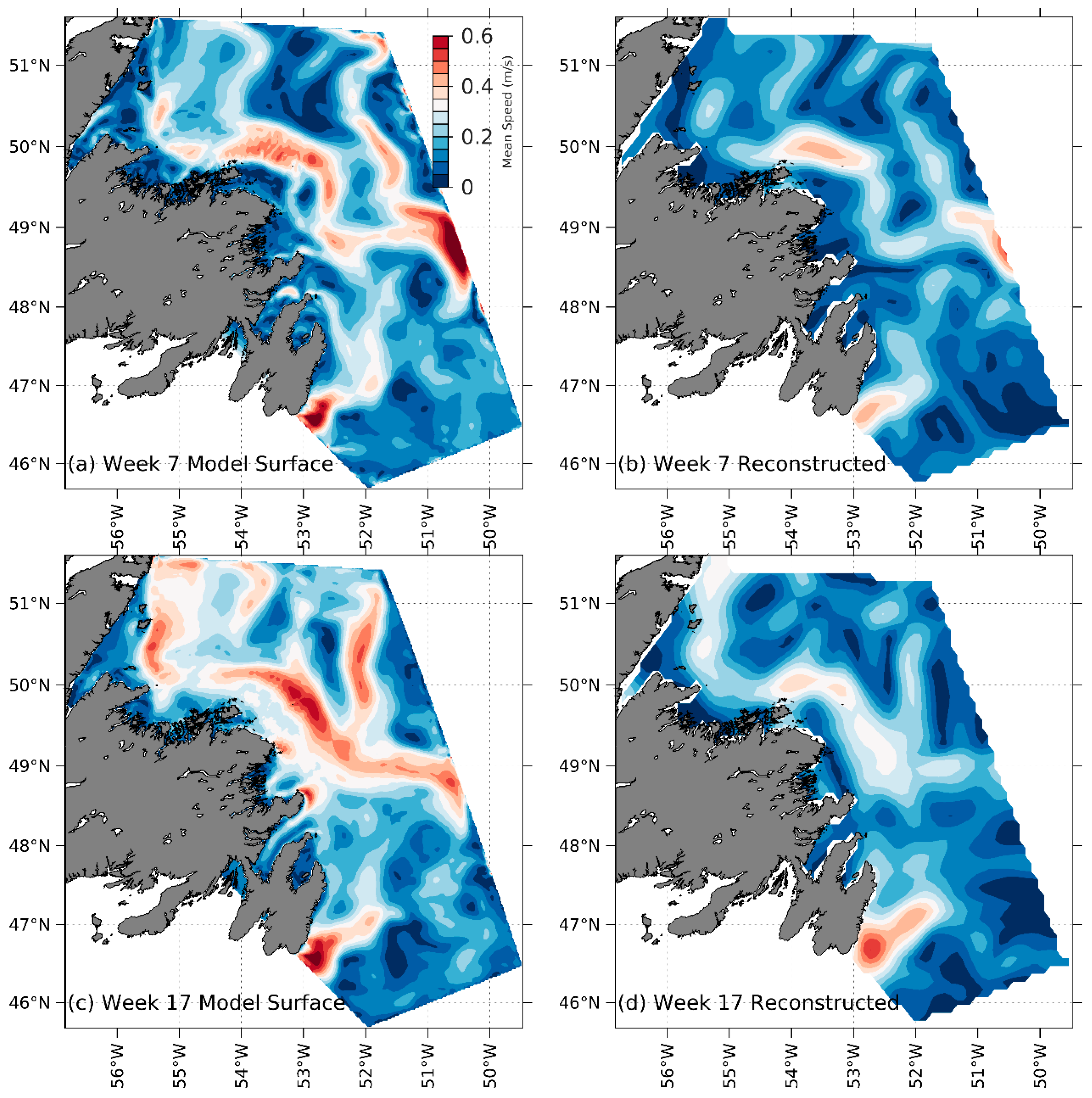
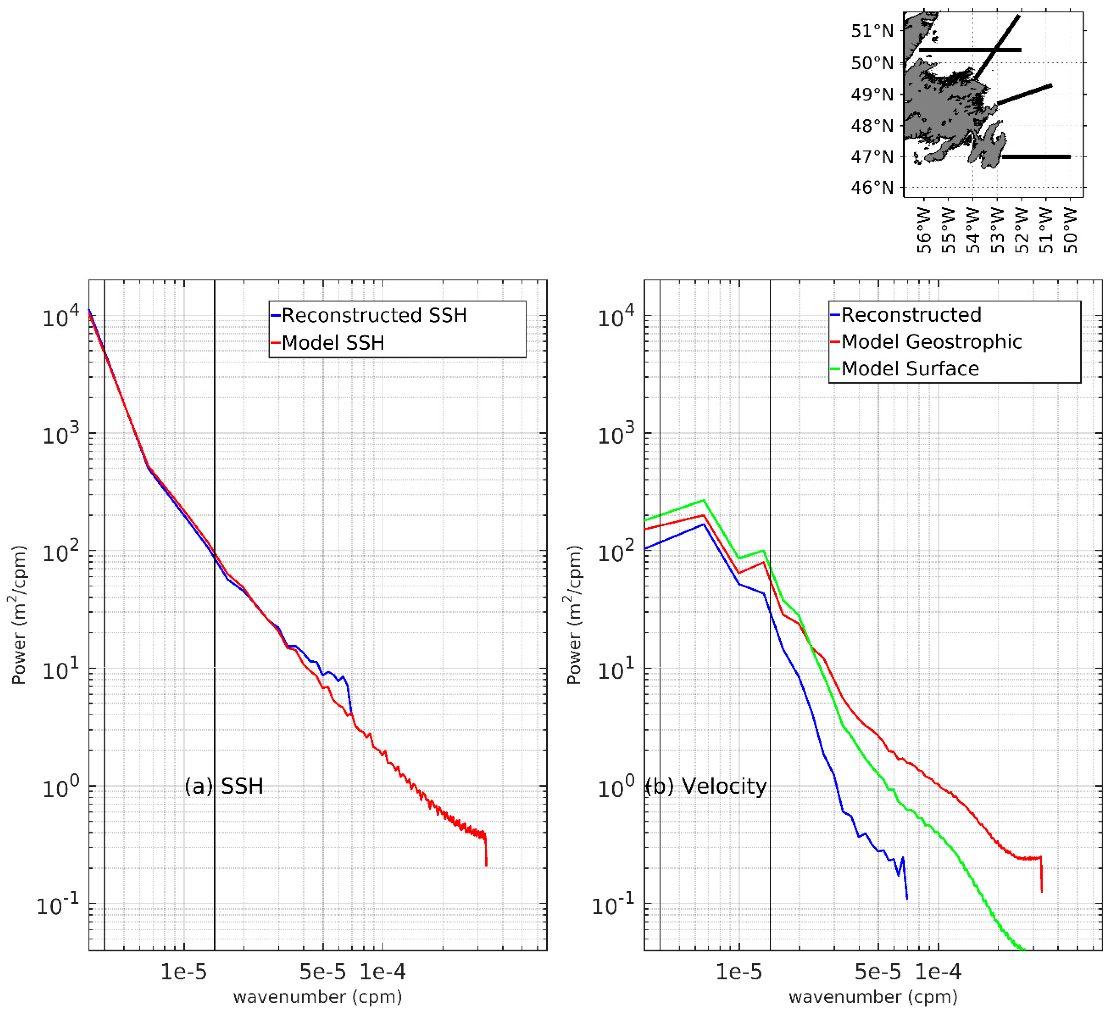
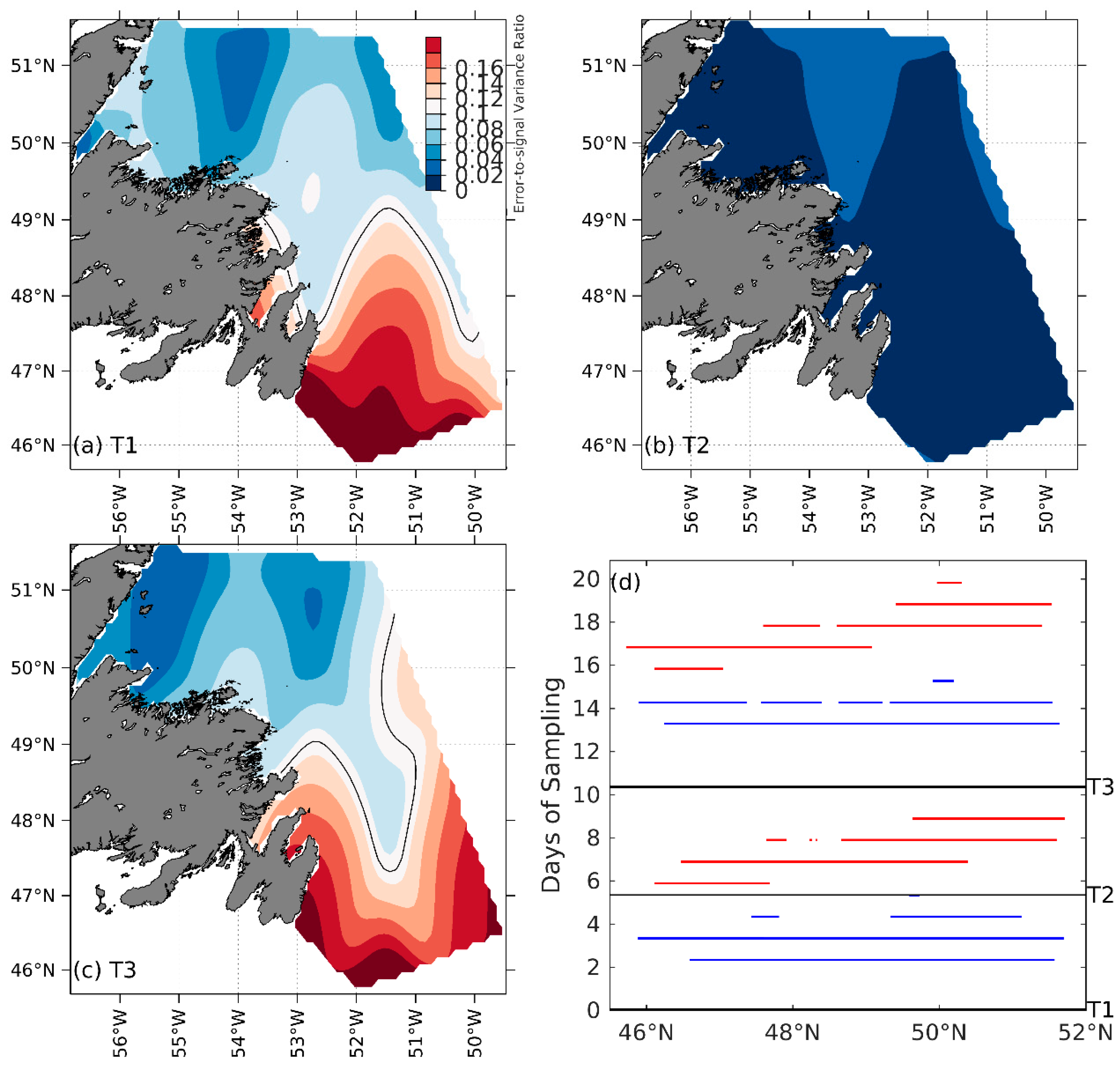
3.2. SWOT Simulation and Reconstruction

To study the reconstructability of the coastal sea level and current off the Newfoundland coast, OI was applied on the simulated SWOT data within a 10-day window onto a 0.1° grid with half-day intervals. We then averaged the half-day mapped SSH fields into weekly fields, which were then compared with the corresponding model SSH averaged from hourly outputs. In total, there were 22 weeks from 1 June 2010 to 31 October 2010. The selection of a 10-day window ensured the data coverages equivalent to one subcycle for each mapped half-day field. Figure 5a,b compares the reconstructed SWOT SSH and the model SSH at week 7 when the reconstructed field has a minimum RMS error of 2.5 cm, while Figure 5c,d shows the two corresponding SSH fields at week 17 when the reconstructed field has a maximum RMS error of 10.8 cm. The mean of the RMS errors for 22 weeks is 4.6 ± 2.2 cm. The cross-shelf SSH slope of the Labrador Current is reasonably reproduced in the reconstructed SSH, with underestimation at week 17 (Figure 5c,d). Sub-mesoscale features such as convergence and divergence are approximately captured (Figure 5a,b). The normalized RMSD (defined as the ratio of the RMS error between the reconstructed SSH and the model SSH to the RMS values of the model SSH) for week 7 and week 17 is about 0.05 and 0.30, respectively. The reconstructed geostrophic surface current, derived from the reconstructed SSH based on a first-order Euler forward difference between two data points, is compared with the model surface current for week 7 and 17 (Figure 6a–d), with their normalized RMSDs at 0.37 and 0.46, respectively. The inshore Labrador Current is fairly represented in the geostrophic surface current derived from the reconstructed SSH, though underestimated to some degree due to hurricane-induced ageostrophic current and the scarcity of SWOT swaths. For all 22 weekly products, the normalized RMSDs range from 0.35 to 0.50, indicating a reasonable agreement in magnitude and spatial variability.

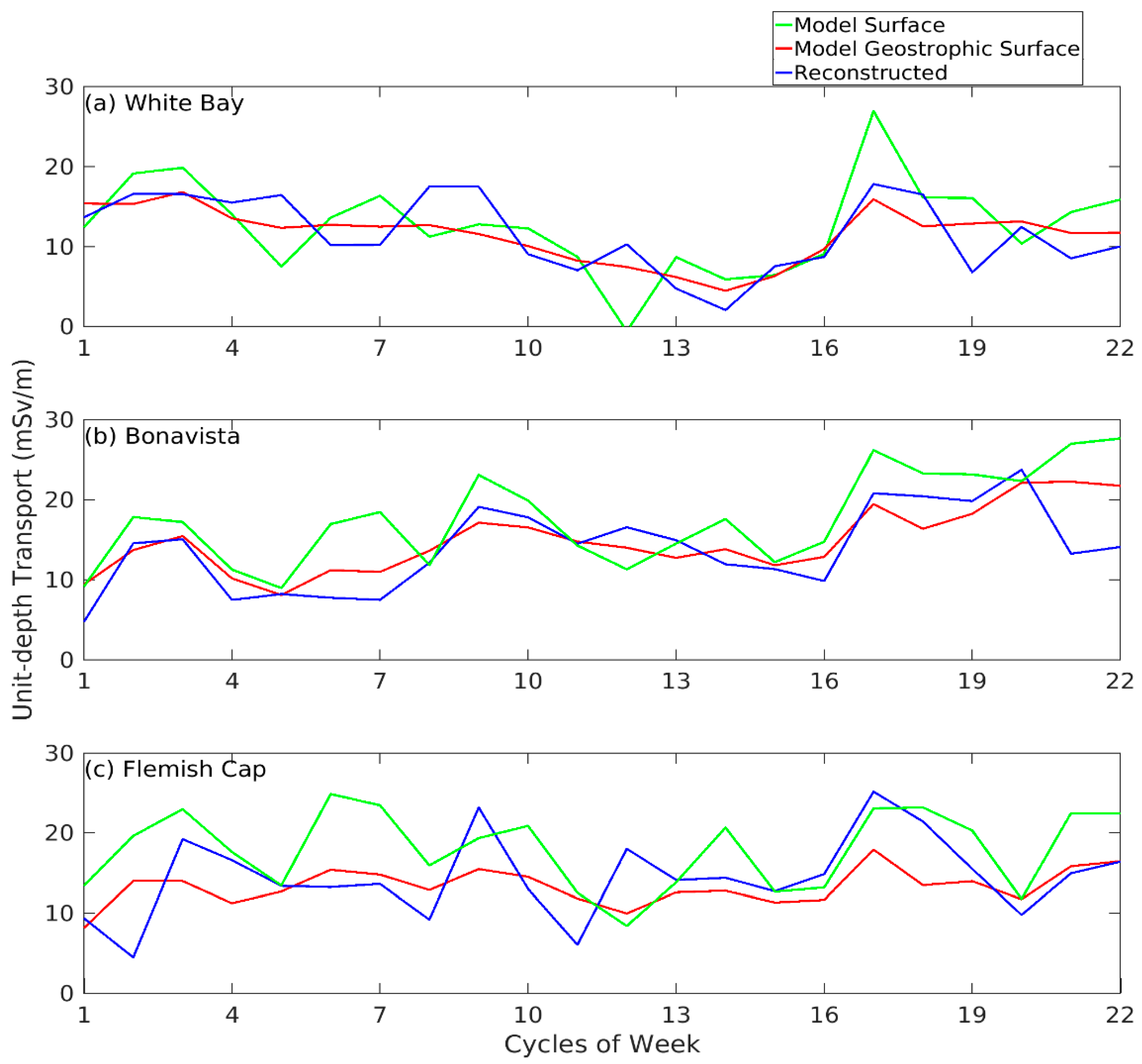
3.3. The Surface Inshore Labrador Current and its Surface Unit-Depth Transport

To assess the reconstructability of the surface inshore Labrador Current, we selected four transects (locations in Figure 7f) approximately perpendicular to the mean pathway of the inshore Labrador Current. The length of the transects ranged from 180 to 300 km, and the averaged SSH and current for the four transects were computed within 180 km from the coast. Figure 7a,b show good agreement between the model and reconstructed SSH, with SSH decreasing offshore. There is also intermittent strong SSH gradient within 100 km from the coast, with largest gradient between 40 to 90 km from the coast. The RMS error between the model and reconstructed SSH is 3.5 cm, with a normalized RMSD of 0.07, indicating good reconstruction of SSH.
The model surface current (Figure 7e) shows that the inshore Labrador Current is located within 100 km from the coast, with substantial temporal variability. The surface inshore Labrador Current is reproduced in the model geostrophic surface current, with reduced temporal variability and expanded width to some degree (Figure 7c). It is further smoothed to a lesser degree in the reconstructed surface current (Figure 7d). The RMS error between the model geostrophic surface current and the model surface current, and the normalized RMSD, are 0.04 m/s and 0.21, respectively. The RMS error between the reconstructed surface current and the model surface current is 0.05 m/s, while the normalized RMSD is 0.26. Overall, the surface inshore Labrador Current is reproduced in the reconstructed surface current.
The spatial variance of the surface inshore Labrador Current can be assessed in frequency domain from mesoscale to sub-mesoscale bands. Power spectra were computed using a Hamming windowed Fast Fourier Transformation (FFT) approach applied over the four transects, zero-padding to the maximum distance of 300 km. At each transect, any remaining spatial mean and trend were removed prior to computing the frequency spectra. It should be noted that the spectrum was limited by the maximum width of 300 km and cut off by the Nyquist frequency of the 0.1° sampling resolution for the reconstructed fields and the 0.02° sampling resolution for model. A fixed mesoscale wavelength band of 70 to 250 km was defined as in [25,26,27]. We show in Figure 8a the model and reconstructed SSH wavenumber spectrum and in Figure 8b the surface velocity counterparts averaged over the four transects. As can be seen from figure, the mapped SSH agrees with model well in the mesoscale band until about 30 km in terms of amplitude and shape of the spectra, demonstrating the reconstructed SSH could properly resolve the 50–100 km surface inshore Labrador Current. On wavelengths smaller than 30 km, the reconstructed SSH appears to have less power spectral density than the model, with steeper slopes as a result of smoothing process. Both model surface current and model geostrophic surface current spectra (red and green lines in Figure 8b) show two peaks at 80 and 153 km, representing the dominant mesoscale wavelengths of the inshore current. Comparing the model surface current and the model geostrophic surface current, we find similar spectral shapes on meso- and submeso-scale bands, with intensified difference at a transition wavelength of about 30 km. The mean geostrophic surface current spectrum derived from mapped SSH (blue lines in Figure 8b) has similar shape and power density to the other two modelled ones till 100 km, with much less power density on wavelengths shorter than 70 km. Peak locations in the model surface current spectra are reasonably reproduced in the reconstructed fields, but with less power density.
Next, we calculated the surface unit-depth transport within 100 km from the coast. We show in Figure 9 the model surface unit-depth transport (green lines), the model geostrophic surface unit-depth transport (red lines), and the reconstructed surface unit-depth transport (blue lines) at the White Bay, Bonavista, and Flemish Cap transects (See Figure 1 for locations). The surface transport clearly shows intra-seasonal variations.
The model geostrophic surface unit-depth transport is generally comparable to the model surface unit-depth transport with some underestimation. The underestimation is relatively large at the Flemish Cap transect, indicating relative importance of ageostrophic component to the surface unit-depth transport at this transect. The RMS errors between the model geostrophic surface unit-depth transport and the model surface unit-depth transport are within 5.7 mSv/m (1 mSv = 103 m3/s) (Table 2). The normalized RMSDs are within 0.31 (Table 2), and the correlation coefficients are larger than 0.77, indicating a good agreement in variabilities between the model geostrophic surface unit-depth transport and the model surface unit-depth transport. The comparison suggests that geostrophy is a reasonable approximation for the surface inshore Labrador Current at the weekly scale. It should be pointed out that the ageostrophic components are significant in the hourly model surface unit-depth transport.
There is a general agreement between the reconstructed surface unit-depth transport and the model surface unit-depth transport at the three transects in terms of magnitude and variabilities. The normalized RMSDs are within 0.38 (Table 2). The correlation coefficients vary from 0.38 to 0.63 (Table 2), with p values less than 0.02 at the White Bay and Bonavista transects and larger than 0.05 at the Flemish Cap transect. The reconstructed unit-depth transport shows artificially enhanced variations compared with the model geostrophic surface unit-depth transport, which can be attributed to SWOT sampling and optimal interpolation. The substantially lower correlation between the reconstructed surface unit-depth transport and the model surface unit-depth transport may be explained by the artificially enhanced variation in the reconstructed surface unit-depth transport.

4. Summary and Discussion

The present study examined the reconstructability of the weekly SSH off eastern Newfoundland and of its associated geostrophic surface inshore Labrador Current from the SWOT interferometer-derived swath SSH information. Our exploration adopted the 2 km resolution outputs from a fully prognostic numerical model serving as the time-evolving oceanic states for the study period from June to October, 2010. The model results successfully captured observed variations when compared with observations at tide-gauge stations and from the Jason-2 altimeter. The subsequent study then utilized the SWOT simulator tool to mimic the temporal and spatial sampling of the SWOT satellite and the instrumental and geophysical errors for the SWOT measurements. To reconstruct SSH fields from SWOT swath information, optimal interpolation with the pre-selected temporal and spatial decorrelation scales was applied. The optimal interpolation (OI) data window was 10 days to include the sufficient SWOT samples. The normalized RMSD of the weekly reconstructed SSH against the model SSH ranged from 0.05 to 0.30. A further examination of the surface speed averaged over the four transects approximately perpendicular to the mean pathway of the inshore current revealed that the inshore Labrador Current was fairly reconstructed within 100 km from the coast in terms of magnitude and temporal variability. The spatial variance of the inshore Labrador Current was presented by computing the wavenumber spectrum. The spectral shape and peaks of the reconstructed surface current and the model geostrophic surface current were compared with those of the model surface current. There was a transition wavelength at about 30 km with increasing difference toward the cut-off between the model surface current and the model geostrophic surface current, while this transition wavelength between the model surface current and the reconstructed surface current was 70–100 km. The reconstructed surface unit-depth transport of the Labrador Current based on the mapped SSH had normalized RMSDs of 0.32–0.38 relative to the corresponding model transport.
The adoption of the objective mapping approach is to minimize the impact of the sampling inadequacy and measurement errors from the SWOT mission. As with many altimetry reconstruction applications (e.g., [11]), the selection of OI in this study seems to be able to reduce the measurement errors effectively. However, because of the gaps between the neighboring swaths, the SSH fields are spatially smoothed, negatively impacting on associated geostrophic surface current and surface unit-depth transport. Thus, there is a need to conduct a posterior error analysis, examining the error-to-signal variance ratios from OI. We select three typical time spots shown in Figure 10d (blacks lines labeled as T1-T3), representing different levels of data coverage. Figure 10a–c shows the variance ratio based on equation (3) that purely accounts for the errors caused by swaths gaps. By looking at Equations (2) and (3), the error-to-signal variance ratio represents the accuracy of OI estimation. As seen from Figure 10, the ratios at T1 and T3 are significantly higher than those at T2, indicating larger deviations of the estimated variance from observations. There are also spatial trends at T1 and T3, with small ratios in the northern part of domain, increasing toward the southern part, as a result of the influence by the coastal geometry together with swath locations.
Although we may encounter high error-to-signal variance ratios from OI at a particular mapping time of each repeated cycle when reconstructing, it is understandable that the weekly variance ratios are fairly low. Therefore, it is also interesting to further compare the weekly error-to-signal variance ratios from OI against the actual error-to-signal ratios between the reconstructed SSH and the model SSH. The actual error-to-signal variance ratio is defined as the ratio of the squared difference between the reconstructed and mode SSHs to the squared model SSH. The selected spatial fields, as shown in Figure 11, are for week 7 and 17, corresponding to the selection in Figure 5. As expected, the weekly variance ratios from OI are quite small, with spatially uniform values below 0.06 for both weeks (Figure 11a,c). Regarding the actual error-to-signal variance ratios, however, there are significant differences between week 7 and week 17 (Figure 11b,d). For week 17, the actual error-to-signal variance ratio is remarkably higher along the coast than the ratio from OI.

5. Conclusions

Overall, our study demonstrates that the coastal SSH fileds for the Labrador Current on the weekly scales can be reconstructed from the SWOT-like data using optimal interpolation with a normalized RMSD of 0.07 between the reconstructed and model SSHs. Nevertheless, the present results show that the discrepancies between the unit-depth transport of the reconstructed surface Labrador Current and the corresponding model transport are larger, with normalized RMSDs of 0.32–0.38 due to the SWOT sampling inadequcy and the geostrophic approximation. As a next step, we have started to work on assimilating the SWOT-like data into a coastal circulation model.

Author Contributions

Z.M. designed the approach, implemented the numerical model and SWOT simulator software, validated the numerical model with observations, conducted the data analysis, and wrote the paper. G.H. conceptualized the study, acquired funding, managed the project, designed the approach, supervised the investigation, and wrote the paper.

Funding

This research was funded by the Surface Water and Ocean Topography—Canada (SWOT-C) Program, Canadian Space Agency.

Acknowledgments

We thank Lucile Gaultier and Clement Ubelmann for advice on the SWOT simulator and Nancy Chen for acquiaring and peocessing the 1-Hz Jason-2 along-track data. The 1-Hz Jason-2 data are from the Radar Altimetry Data System (RADS) (http://rads.tudelft.nl/rads/rads.shtml). The altimetry gridded data are from the Copernicus Marine and Environment Monitoring Service (CMEMS) (http://marine.copernicus.eu). The work is supported by Compute Canada. Helpful comments and suggestions were received from the reviewers.

Conflicts of Interest

The authors declare no conflict of interest.

References

  1. Greenberg, D.A.; Petrie, B.D. The mean barotropic circulation on the Newfoundland Shelf and slope. J. Geophys. Res. 1988, 93, 15541–15550. [Google Scholar] [CrossRef]
  2. Han, G.; Lu, Z.; Wang, Z.; Helbig, J.; Chen, N.; de Young, B. Seasonal variability of the Labrador Current and shelf circulation off Newfoundland. J. Geophs. Res. 2008, 113. [Google Scholar] [CrossRef]
  3. Ma, Z.; Han, G.; Chassé, J. Simulation of circulation and ice over the Newfoundland and Labrador Shelves: the mean and seasonal cycle. Atmos.Ocean. 2015, 54, 248–263. [Google Scholar] [CrossRef]
  4. Han, G.; Ikeda, M. Basin-scale variability in the Labrador Sea from TOPEX/Poseidon and Geosat altimeter data. J. Geophys. Res. 1996, 101, 28325–28334. [Google Scholar] [CrossRef]
  5. Han, G.; Tang, C.L. Velocity and transport of the Labrador Current determined from altimetric, hydrographic, and wind data. J. Geophs. Res. 1999, 194, 18,047–18,057. [Google Scholar] [CrossRef]
  6. Han, G.; Tang, C.L. Interannual variations of volume transport in the western Labrador Sea based on TOPEX/Poseidon and WOCE data. J. Phys. Oceanogr. 2001, 31, 199–211. [Google Scholar] [CrossRef]
  7. Häkkinen, S.; Rhines, P.B. Decline of subpolar North Atlantic circulation during the 1990s. Science 2004, 304, 555–559. [Google Scholar] [CrossRef]
  8. Lazier, J.R.N.; Wright, D.G. Annual velocity variations in the Labrador Current. J. Phys. Oceanogr. 1993, 23, 659–678. [Google Scholar] [CrossRef]
  9. Chavanne, C.P.; Klein, P. Can oceanic submesoscale processes be observed with satellite altimetry? Geophys. Res. Lett. 2010, 37. [Google Scholar] [CrossRef] [Green Version]
  10. Chelton, D.; Schlax, M. The accuracies of smoothed sea surface height fields constructed from tandem altimeter datasets. J. Atmos, Oceanic Technol. 2003, 20, 1276–1302. [Google Scholar] [CrossRef]
  11. Fu, L.L.; Ubelmann, C. On the transition from profile altimetry to swath altimeter for observation global ocean surface topography. J. Atmos. Oceanic Technol. 2014, 31, 560–568. [Google Scholar] [CrossRef]
  12. Han, G.; Ma, Z.; de Young, B.; Foreman, M.; Chen, N. Simulation of three-dimensional circulation and hydrography over the Grand Banks of Newfoundland. Ocean Model. 2011, 40, 199–210. [Google Scholar] [CrossRef]
  13. Ma, Z.; Han, G.; de Young, B. Oceanic responses to Hurricane Igor over the Grand Banks: A modeling study. J. Geophs. Res. 2015, 120, 1276–1295. [Google Scholar] [CrossRef]
  14. Saha, S.; Moorthi, S.; Pan, H.; Wu, X.; Wang, J.; Nadiga, S.; Tripp, P.; Kistler, R.; Woollen, J.; Behringer, D.; et al. The NCEP Climate Forecast System Reanalysis (CFSR). Bull. Amer. Meteor. Sco. 2010, 91, 1015–1057. Available online: https://doi.org/10.5065/D6513W89 (accessed on 14 July 2018). [CrossRef]
  15. Gaultier, L.; Ubelmann, C.; Fu, L.-L. The chanllenge of using future SWOT data for oceanic field reconstruction. J. Atmos. Oceanic Technol. 2015, 33, 119–126. [Google Scholar] [CrossRef]
  16. Pawlowicz, R.; Beardsley, B.; Lentz, S. Classical tidal harmonic analysis including error estimates in MATLAB using T_TIDE. Comput. Geosci. 2002, 28, 929–937. [Google Scholar] [CrossRef]
  17. Bretherton, F.P.; Davis, R.E.; Fandry, C.B. A technique for objective analysis and design of oceanographic experiments applied to MODE-73. Deep-Sea Res. 1976, 23, 559–582. [Google Scholar] [CrossRef]
  18. Qiu, B.; Chen, S.; Klein, P.; Ubelmann, C.; Fu, L.-L. Reconstructability of three-dimensional upper-ocean circulation from SWOT sea surface height measurements. J. Phys. Oceanogr. 2016, 46, 947–963. [Google Scholar] [CrossRef]
  19. Le Traon, P.Y.; Hernandez, F. Mapping the oceanic mesoscale circulation: validation of satellite altimetry using surface drifters. J. Atmos, Oceanic Technol. 1992, 9, 687–698. [Google Scholar] [CrossRef]
  20. Ubelmann, C.; Cornuelle, B.; Fu, L.-L. Dynamic mapping of along-track ocean altimetry: method and performance from observing system simulation experiments. J. Atmos. Oceanic Technol. 2016, 33, 1691–1699. [Google Scholar] [CrossRef]
  21. Ruggiero, G.A.; Cosme, E.; Brankart, J.-M.; Sommer, J.L.; Ubelmann, C. An efficient way to account for observation error correlations in the assimilations of data from the future SWOT High-Resolution altimeter mission. J. Atmos, Oceanic Technol. 2016, 33, 2755–2768. [Google Scholar] [CrossRef]
  22. Han, G.; Ohashi, K.; Chen, N.; Myers, P.G.; Nunes, N.; Fischer, J. Decline and partial rebound of the Labrador Current 1993-2004: monitoring ocean currents from altimetric and CTD data. J. Geophs. Res. 2010, 115. [Google Scholar] [CrossRef]
  23. Behnisch, M.; Macrander, A.; Boebel, O.; Wolff, J.-O.; Schroter, J. Barotropic and deep-referenced baroclinic SSH variability derived from Pressure Inverted Echo Sounders (PIES) south of Africa. J.Geophs.Res.Oceans. 2013, 118, 3046–3058. [Google Scholar] [CrossRef]
  24. Petrie, B.; Anderson, C. Circulation on the newfoundland continental shelf. Atmos.-Ocean. 1983, 21, 207–226. [Google Scholar] [CrossRef]
  25. Le Traon, P.Y.; Klein, P.; Hua, B.L.; Dibarboure, G. Do altimeter wavenumber spectra agree with the interior or surface quasigeostrophic theory? J. Phys, Oceanogr. 2008, 38, 1137–1142. [Google Scholar] [CrossRef]
  26. Xu, Y.; Fu, L.-L. Global variability of the wavenumber spectrum of oceanic mesoscale turbulence. J. Phys. Oceanogr. 2011, 41, 802–809. [Google Scholar] [CrossRef]
  27. Xu, Y.; Fu, L.-L. The effect of altimeter instrument noise on the estimation of the wavenumber spectrum of sea surface height. J. Phys. Oceanogr. 2012, 42, 2229–2233. [Google Scholar] [CrossRef]
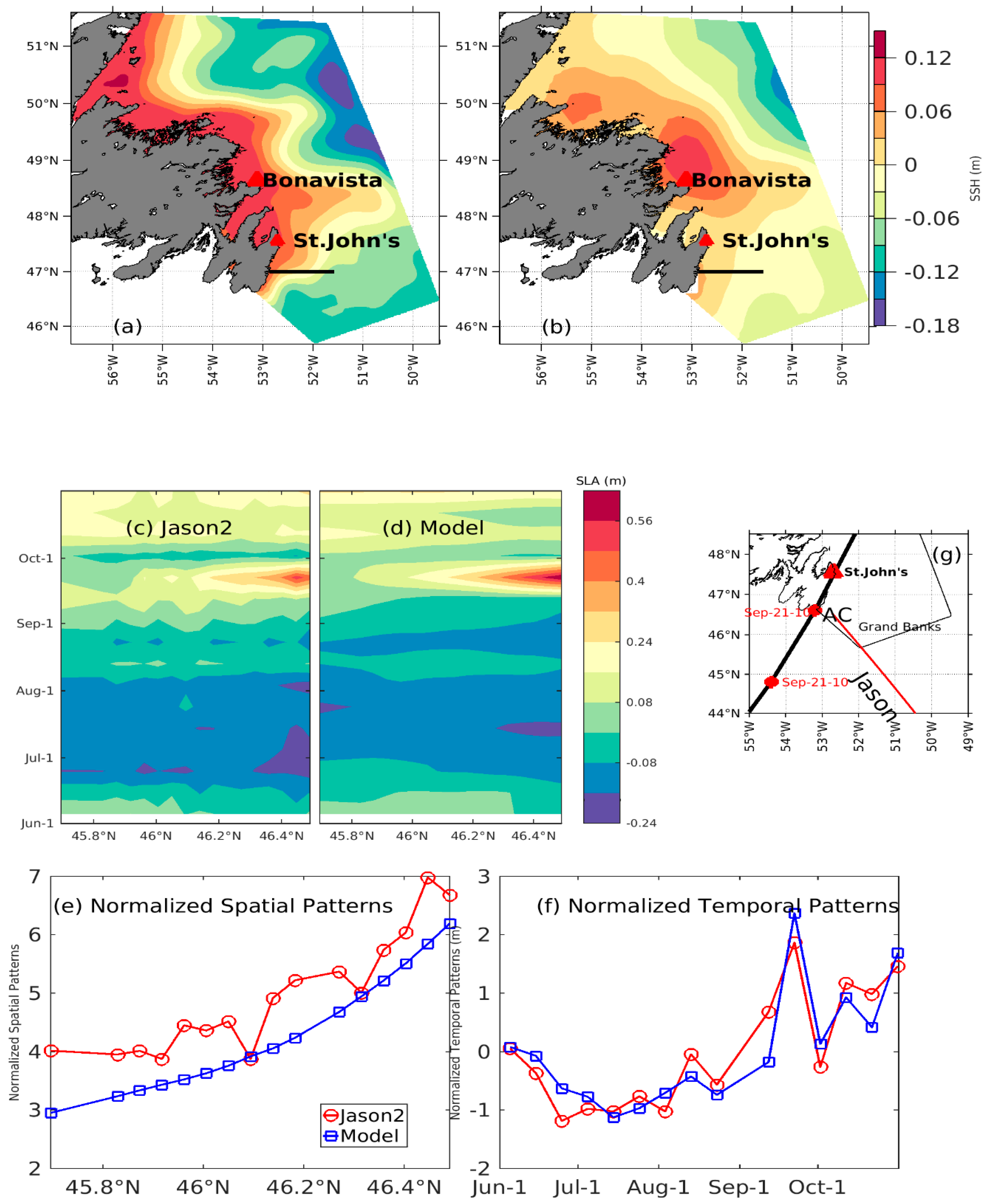
Figure 1. Map showing the Newfoundland Shelf off the eastern Newfoundland coast as well as the model boundaries (thick solid lines). The isobaths displayed are 100 (red line) and 200 (blue line) m. AC is the Avalon Channel. NL is Newfoundland. Three transects are White Bay, Bonavista, and Flemish Cap. Two red triangles indicate tide-gauge stations.
Remotesensing 11 01264 g001
Figure 2. Spatial swath distribution within one repeat cycle of the Surface Water and Ocean Topography (SWOT) mission off eastern Newfoundland: (a) the first subcycle and (b) the second subcycle. (c) Ascending swath passes (red lines) and descending swath passes (blue lines) inside the domain as a function of time and latitude. Black lines in (a) and (b) are the border of the model domain. The unit of color band in (a) and (b) is days in the cycle.
Remotesensing 11 01264 g002
Figure 3. (a) Five-month averaged sea surface height (SSH) field off eastern Newfoundland from Finite Volume Community Ocean Model (FVCOM) with its spatial mean removed. (b) Five-month averaged absolute dynamic topography derived from multi-mission altimeter data with its spatial mean removed. (c) Jason-2 and (d) model sea level anomaly (de-tided) from 1 June 2010 to 31 October 2010. (e) Normalized Empirical Orthogonal Function (EOF) mode 1 spatial patterns calculated by the first EOF spatial patterns over its own standard deviation. (f) As in (e) but for temporal patterns. (g) One of the Jason-2 satellite ground tracks (Red) and storm track (Black) with model open boundary. AC in (g) is Avalon Channel. Black thick lines in (a) and (b) indicate locations to estimate the mean magnitude of the inshore Labrador Current.
Remotesensing 11 01264 g003
Figure 4. Hourly de-tided sea level anomalies from tide-gauge observations (red) and model results at (a) Bonavista and (b) St. John’s. The vertical line depicts the landfall time of Hurricane Igor.
Remotesensing 11 01264 g004
Figure 5. The model SSH for (a) the 7th week and (c) the 17th week and the mapped SSH using optimal interpolation for (b) the 7th week and (d) the 17th week.
Remotesensing 11 01264 g005
Figure 6. Mean model surface current for (a) the 7th week and (c) the 17th week. (b) and (d) as in (a) and (c), but for mean reconstructed surface current derived from the mapped SSH.
Remotesensing 11 01264 g006
Figure 7. Hovmöller diagram of (a) model SSH, (b) reconstructed SSH, (c) model geostrophic surface current, (d) reconstructed surface current, and (e) model surface current averaged over four transects within 180 km from the coast. The transects are approximately perpendicular to the mean pathway of the inshore current, with locations indicated by the black lines in (f).
Remotesensing 11 01264 g007
Figure 8. Wavenumber spectrum (a) of mapped SSH (blue lines) and model (red lines) and (b) of the mapped SSH-derived geostrophic surface current (blue lines), model SSH-derived ones (red lines), and model surface current (green lines) averaged over the four transects. The areas between two black lines indicate mesoscale band (70 to 250 km) defined as in [25,26,27].
Remotesensing 11 01264 g008
Figure 9. The weekly surface unit-depth Labrador Current transport at the (a) White Bay, (b) Bonavista, and (c) Flemish Cap transects.
Remotesensing 11 01264 g009
Figure 10. Residual variance ratio at (a) T1, (b) T2, and (c) T3 indicated as black lines in (d) ascending swath passes (red lines) and descending swath passes (blue lines) inside the region as a function of time and latitude. Black contours from (a)–(c) are the boundary lines of 0.11.
Remotesensing 11 01264 g010
Figure 11. Residual variance ratio from OI for (a) week 7 and (c) week 17, and the ratio of residual variance to model variance for (b) week 7 and (d) week 17.
Remotesensing 11 01264 g011
Table 1. Statistics comparing the first EOF mode of Jason-2 and model sea level anomaly from 1 June 2010 to 31 October 2010 with their spatial and temporal standard deviations and root-mean-square errors of their normalized values. Normalized values are defined as the ratio of the first mode patterns to its own standard deviation.
Spatial Standard DeviationRoot-Mean-Square Error of Normalized Spatial PatternsTemporal Standard Deviation (m)Root-Mean-Square Error of Normalized Temporal Patterns
Jason-20.050.730.540.40
Model0.060.55
Table 2. Statistics comparing the reconstructed surface unit-depth transport and the model geostrophic surface unit-depth transport against the model surface unit-depth transport at the White Bay, Bonavista, and Flemish Cap transects. Locations are shown in Figure 1.
Reconstructed Transport Versus Model TransportModel Geostrophic Transport Versus Model Transport
RMS ErrorUnit: mSv/mNormalized RMSDCorrelation CoefficientRMS ErrorUnit: mSv/mNormalized RMSDCorrelation Coefficient
White Bay5.30.380.493.90.280.77
Bonavista6.00.320.634.10.220.87
Flemish Cap6.50.350.385.70.310.80

